Questions as text
Q1 · The stem-and-leaf diagram below represents data collected for the number of hits on an… 9709/61 May/June 2008
1 The stem-and-leaf diagram below represents data collected for the number of hits on an internet site on each day in March 2007. There is one missing value, denoted by x. 0 0 1 5 6 (4) 1 1 3 5 6 6 8 (6) 2 1 1 2 3 4 4 4 8 9 (9) 3 1 2 2 2 x 8 9 (7) 4 2 5 6 7 9 (5) Key: 1 5 represents 15 hits (i) Find the median and lower quartile for the number of hits each day. [2] (ii) The interquartile range is 19. Find the value of x. [2]
4 marks
Mark scheme: 1 (i) median = 16th along = 24 B1 LQ = 16 not 15.5 B1 2 (ii) UQ = LQ + 19 = 35 M1 For adding 19 to their LQ in whatever form x = 5 A1 2 Must be 5 not 35. c.w.o.
This question in 9709/61 May/June 2008
Q2 · As part of a data collection exercise, members of a certain school year group were asked… 9709/61 May/June 2008
5 As part of a data collection exercise, members of a certain school year group were asked how long they spent on their Mathematics homework during one particular week. The times are given to the nearest 0.1 hour. The results are displayed in the following table. Time spent (t hours) 0.1 ≤t ≤0.5 0.6 ≤t ≤1.0 1.1 ≤t ≤2.0 2.1 ≤t ≤3.0 3.1 ≤t ≤4.5 Frequency 11 15 18 30 21 (i) Draw, on graph paper, a histogram to illustrate this information. [5] (ii) Calculate an estimate of the mean time spent on their Mathematics homework by members of this year group. [3]
8 marks
Mark scheme: 5 (i) fd: 22, 30, 18, 30, 14 M1 Attempt at freq density or scaling fd A1 correct heights seen on graph 30 B1 Bar lines correctly located at 0.55, 1.05, 2.05, 3.05, no gaps 20 B1 correct widths of bars 10 B1 5 both axes uniform from at least 0 to 15 or 30, and 0.05 to 4.5 and labelled, (fd, or 0 1 2 3 4 5 time freq per half hour , time, hours, t) (ii) mid-points 0.3, 0.8, 1.55, 2.55, 3.8 M1 an attempt at mid-points (not class widths) = 199.5 / 95 M1 using (Σ their fx) / their 95 mean = 2.1 hours A1 3 correct answer from 199.5 in num
This question in 9709/61 May/June 2008
Q3 · Rachel measured the lengths in millimetres of some of the leaves on a tree 9709/61 Oct/Nov 2008
1 Rachel measured the lengths in millimetres of some of the leaves on a tree. Her results are recorded below. 32 35 45 37 38 44 33 39 36 45 Find the mean and standard deviation of the lengths of these leaves. [3]
3 marks
Mark scheme: 1 mean = 38.4 mm B1 Correct answer M1 Correct method if shown (can be implied)must see a sign sd = 4.57 mm c.a.o A1 [3] Correct answer
This question in 9709/61 Oct/Nov 2008
Q4 · The pulse rates, in beats per minute, of a random sample of 15 small animals are shown in… 9709/61 Oct/Nov 2008
5 The pulse rates, in beats per minute, of a random sample of 15 small animals are shown in the following table. 115 120 158 132 125 104 142 160 145 104 162 117 109 124 134 (i) Draw a stem-and-leaf diagram to represent the data. [3] (ii) Find the median and the quartiles. [2] (iii) On graph paper, using a scale of 2 cm to represent 10 beats per minute, draw a box-and-whisker plot of the data. [3]
8 marks
Mark scheme: 5 (i) 10 4 4 9 B1 Correct stem 11 5 7 12 0 4 5 13 2 4 B1 Correct leaves, must be sorted and in columns 14 2 5 and give correct overall shape 15 8 16 0 8 key 10 4 represents 104 B1 [3] Key, must have vertical line in both (ii) median = 125 B1 Any 2 correct values seen LQ = 115 UQ = 145 B1 [2] third correct value (iii) B1 correct uniform scale from at least 110 to 160 with room for end points, and label or title B1ft correct median and quartiles on diagram ft their values (must be box ends) 100 110 120 130 140 150 160 170 pulse rate B1 [3] correct whiskers, no line through box, touching box in the middle not the top or bottom GCE A/AS LEVEL – October/November 2008 9709 06
This question in 9709/61 Oct/Nov 2008
Q5 · During January the numbers of people entering a store during the first hour after opening… 9709/61 May/June 2009
6 During January the numbers of people entering a store during the first hour after opening were as follows. Time after opening, Frequency Cumulative x minutes frequency 0 < x ≤10 210 210 10 < x ≤20 134 344 20 < x ≤30 78 422 30 < x ≤40 72 a 40 < x ≤60 b 540 (i) Find the values of a and b. [2] (ii) Draw a cumulative frequency graph to represent this information. Take a scale of 2 cm for 10 minutes on the horizontal axis and 2 cm for 50 people on the vertical axis. [4] (iii) Use your graph to estimate the median time after opening that people entered the store. [2] (iv) Calculate estimates of the mean, m minutes, and standard deviation, s minutes, of the time after opening that people entered the store. [4] (v) Use your graph to estimate the number of people entering the store between (m −12s) and (m + 12s) minutes after opening. [2]
14 marks
Mark scheme: 6 (i) a = 494 B1 b = 46 B1 [2] (ii) B1 Correct linear scale minimum 0 to 540 and 0 to 60 B1 Labels (cf or people or number of people) and (time, or minutes) and attempt at cf or cf step polygon M1 Attempt to plot points at (10, 210), (20, 344), (30, 422), (40, 494) A1 [4] Correct graph through (0, 0) and (60, 540) (iii) median is M1 Attempt to read from graph at line y = 270 or 270.5 13.5 to 14.6 min A1 [2] Correct answer (iv) (5 × 210 + 15 × 134 + 25 × 78 + M1 Using mid points and frequencies 35 × 72 + 50 × 46) / 540 = 9830 / 540 = 18.2 min A1 Correct mean (52 × 210 + 152 × 134 + … ) – 18.22 M1 Attempt at Σx2f / Σf – their mean2 numerically, could use cfs, ucb, but not class widths sd = 14.2 min A1 [4] Correct answer (v) 18.2 ± 7.1 = 11.1, 25.3 M1 Attempt to read their mean ± ½ sd from cf graph 390 – 225 = 155 to 170 people A1 [2] Correct answer
This question in 9709/61 May/June 2009
Q6 · A library has many identical shelves 9709/61 Oct/Nov 2009
4 A library has many identical shelves. All the shelves are full and the numbers of books on each shelf in a certain section are summarised by the following stem-and-leaf diagram. 3 3 6 9 9 (4) 4 6 7 (2) 5 0 1 2 2 (4) 6 0 0 1 1 2 3 4 4 4 4 4 5 5 6 6 6 7 8 8 9 (20) 7 1 1 3 3 3 5 6 6 7 8 9 9 (12) 8 0 2 4 5 5 6 8 (7) 9 0 0 1 2 4 4 4 4 5 5 6 7 7 8 8 9 9 9 (18) Key: 3 6 represents 36 books (i) Find the number of shelves in this section of the library. [1] (ii) Draw a box-and-whisker plot to represent the data. [5] In another section all the shelves are full and the numbers of books on each shelf are summarised by the following stem-and-leaf diagram. 2 1 2 2 2 3 3 4 5 6 6 6 7 9 (13) 3 0 1 1 2 3 4 4 5 6 6 7 7 7 8 8 (15) 4 2 2 3 5 7 7 8 9 (8) Key: 3 6 represents 36 books (iii) There are fewer books in this section than in the previous section. State one other difference between the books in this section and the books in the previous section. [1]
7 marks
Mark scheme: 4 (i) 67 B1 [1] (ii) LQ = 64 M1 Attempt to find all 3 quartiles can be implied Med = 73 UQ = 90 B1 Correct end whiskers (not dots or boxes), not through box, must look accurate B1 Correct median line in box must look accurate B1 Correct box ends must look accurate
This question in 9709/61 Oct/Nov 2009
Q7 · 39 63 wind speed (km h–1) Measurements of wind speed on a certain island were taken over… 9709/62 Oct/Nov 2009
1 39 63 wind speed (km h–1) Measurements of wind speed on a certain island were taken over a period of one year. A box-and- whisker plot of the data obtained is displayed above, and the values of the quartiles are as shown. It is suggested that wind speed can be modelled approximately by a normal distribution with mean µ km h−1 and standard deviation σ km h−1. (i) Estimate the value of µ. [1] (ii) Estimate the value of σ. [3]
4 marks
Mark scheme: 1 (i) mean = 51 B1 [1] (ii) z = ±0.674 B1 Correct z ±(63 – 51) / σ = 0.674 M1 Standardising, no cc, no σ , no σ2 σ = 17.8 A1 [3] Correct answer
This question in 9709/62 Oct/Nov 2009
Q8 · The following table gives the marks, out of 75, in a pure mathematics examination taken… 9709/62 Oct/Nov 2009
6 The following table gives the marks, out of 75, in a pure mathematics examination taken by 234 students. Marks 1–20 21–30 31–40 41–50 51–60 61–75 Frequency 40 34 56 54 29 21 (i) Draw a histogram on graph paper to represent these results. [5] (ii) Calculate estimates of the mean mark and the standard deviation. [4]
9 marks
Mark scheme: 6 (i) class widths 20, 10, 10, 10, 10, 15 freq density: 2.0, 3.4, 5.6, 5.4, 2.9, 1.4 M1 Attempt at fd or scaled frequency fd A1 Correct heights seen on graph B1 Bar lines correctly located at 20.5, 30.5, 40.5, 50.5 and 60.5, no gaps B1 Correct widths of bars B1 Both axes uniform from at least 0 to 5.6 and 0.5 to 75.5 and labelled (fd or fr per mark, marks) 0.5 20.5 … etc … 60.5 75.5 marks [5] (ii) mid-points 10.5, 25.5, 35.5, 45.5, 55.5, 68 M1 Attempt at Σxf / 234 using mid-points, NOT class mean = Σxf / 234 = 8769.5/234 widths, NOT upper class bounds = 37.5 A1 Correct answer var = Σx2f / 234 – mean2 M1 Numerical attempt at correct variance formula, NOT class widths sd = 16.9 A1 [4] Correct answer 128 −125
This question in 9709/62 Oct/Nov 2009
Q9 · The numbers of people travelling on a certain bus at different times of the day are as… 9709/61 May/June 2010
2 The numbers of people travelling on a certain bus at different times of the day are as follows. 17 5 2 23 16 31 8 22 14 25 35 17 27 12 6 23 19 21 23 8 26 (i) Draw a stem-and-leaf diagram to illustrate the information given above. [3] (ii) Find the median, the lower quartile, the upper quartile and the interquartile range. [3] (iii) State, in this case, which of the median and mode is preferable as a measure of central tendency, and why. [1]
7 marks
Mark scheme: 2 (i) B1 Correct stem Key 0 2 5 6 8 8 1 2 represents B1 Correct leaves must be sorted and 1 2 4 6 7 7 9 12 people accurate 2 1 2 3 3 3 5 6 7 3 1 5 B1 Key; must have people o.e [3] (ii) median = 19 people B1 Correct median LQ = 10, UQ = 24 B1 Correct quartiles IQ range = 24 – 10 = 14 people B1ft Ft their quartiles [3] (iii) median because mode could be any number B1 Correct answer must say something about which is duplicated more than twice [1] the mode being not much use or another sensible reason
This question in 9709/61 May/June 2010
Q10 · The numbers of rides taken by two students, Fei and Graeme, at a fairground are shown in… 9709/61 May/June 2010
4 The numbers of rides taken by two students, Fei and Graeme, at a fairground are shown in the following table. Roller Water Revolving coaster slide drum Fei 4 2 0 Graeme 1 3 6 (i) The mean cost of Fei’s rides is $2.50 and the standard deviation of the costs of Fei’s rides is $0. Explain how you can tell that the roller coaster and the water slide each cost $2.50 per ride. [2] (ii) The mean cost of Graeme’s rides is $3.76. Find the standard deviation of the costs of Graeme’s rides. [5]
7 marks
Mark scheme: 4 (i) sd = 0 B1* Must see this and some relevant comment, e.g. no change so all rides must cost the same i.e. the mean. B1 dep o.e. [2] (ii) 1 × 2.5 + 3 × 2.5 + 6 × x = 3.76 × 10 M1 attempt to find cost of revolving drum ride 6x = 37.6 – 10 A1 correct equation x = 4.6 for revolving drum A1 correct x σ2 = (2.52 × 1 + 2.52 × 3 + 4.62 × 6)/10 – 3.76 2 M1 substituting in correct variance formula σ = 1.03 A1 correct answer [5] GCE AS/A LEVEL – May/June 2010 9709 61 2 6 8 8
This question in 9709/61 May/June 2010
Q11 · The heights, x cm, of a group of 82 children are summarised as follows 9709/63 May/June 2010
2 The heights, x cm, of a group of 82 children are summarised as follows. Σ(x −130) = −287, standard deviation of x = 6.9. (i) Find the mean height. [2] (ii) Find Σ(x −130)2. [2]
4 marks
Mark scheme: 2 (i) x = 130 − 287 / 82 M1 287/82 seen added or subt to 130 OR 287 seen added or subt to 82 × 130 = 126.5 (126, 127) cm A1 Correct answer [2] Σ ( x − 130) 2 2 2 (ii) − ( −5.3 ) = 9.6 M1 6.92 + (±their coded mean)2 seen or implied 82 Σ(x – 130)2 = 4908.5 cm (4910) A1 correct answer [2] 7 6 7
This question in 9709/63 May/June 2010
Q12 · The lengths of some insects of the same type from two countries, X and Y, were measured 9709/63 May/June 2010
6 The lengths of some insects of the same type from two countries, X and Y, were measured. The stem-and-leaf diagram shows the results. Country X Country Y (10) 9 7 6 6 6 4 4 4 3 2 80 (18) 8 8 8 7 7 6 6 5 5 5 4 4 3 3 3 2 2 0 81 1 1 2 2 3 3 3 5 5 6 7 8 9 (13) (16) 9 9 9 8 8 7 7 6 5 5 3 2 2 1 0 0 82 0 0 1 2 3 3 3 q 4 5 6 6 7 8 8 (15) (16) 8 7 6 5 5 5 3 3 2 2 2 1 1 1 0 0 83 0 1 2 2 4 4 4 4 5 5 6 6 7 7 7 8 9 (17) (11) 8 7 6 5 5 4 4 3 3 1 1 84 0 0 1 2 4 4 5 5 6 6 7 7 7 8 9 (15) 85 1 2 r 3 3 5 5 6 6 7 8 8 (12) 86 0 1 2 2 3 5 5 5 8 9 9 (11) Key: 5 | 81 | 3 means an insect from country X has length 0.815 cm and an insect from country Y has length 0.813 cm. (i) Find the median and interquartile range of the lengths of the insects from country X. [2] (ii) The interquartile range of the lengths of the insects from country Y is 0.028 cm. Find the values of q and r. [2] (iii) Represent the data by means of a pair of box-and-whisker plots in a single diagram on graph paper. [4] (iv) Compare the lengths of the insects from the two countries. [2]
10 marks
Mark scheme: 6 (i) for X: Median = 0.825 cm B1 Correct median IQ range = 0.019 cm (0.833 – 0.814) B1 Correct IQ range [2] (ii) q = 4 B1 r = 2 B1 Must be 4 and 2 not 3 and 1 [2] SR q = 0.824 and r = 0.852 B1 (iii) B1 Labels X, Y and length/cm, linear scale Y from 0.80 to 0.87 and both on one diagram X B1ft Correct median and quartiles for X ft theirs must be a box B1ft Correct median and quartiles for Y ft theirs must be a box 0.80 0.81 0.82 0.83 0.84 0.85 0.86 0.87 B1 Whiskers correct no line through middle length in cm [4] (iv) Y has longer insects on average B1 Correct statement about lengths Y has larger range B1 Correct statement about spreads [2] 135 − µ
This question in 9709/63 May/June 2010
Q13 · Anita made observations of the maximum temperature, t ◦C, on 50 days 9709/61 Oct/Nov 2010
1 Anita made observations of the maximum temperature, t ◦C, on 50 days. Her results are summarised by Σ t = 910 and Σ(t −t)2 = 876, where t denotes the mean of the 50 observations. Calculate t and the standard deviation of the observations. [3]
3 marks
Mark scheme: 1 mean = 18.2 B1 sd = 876 / 50 M1 Correct unsimplified expression seen = 4.19 A1 Correct answer [3]
This question in 9709/61 Oct/Nov 2010
Q14 · The weights in grams of a number of stones, measured correct to the nearest gram, are… 9709/61 Oct/Nov 2010
4 The weights in grams of a number of stones, measured correct to the nearest gram, are represented in the following table. Weight (grams) 1 −10 11 −20 21 −25 26 −30 31 −50 51 −70 Frequency 2x 4x 3x 5x 4x x A histogram is drawn with a scale of 1 cm to 1 unit on the vertical axis, which represents frequency density. The 1 −10 rectangle has height 3 cm. (i) Calculate the value of x and the height of the 51 −70 rectangle. [4] (ii) Calculate an estimate of the mean weight of the stones. [3]
7 marks
Mark scheme: 4 (i) 3 = 2x / 10 M1 Attempt at using freq density = freq / cw x = 15 A1 Correct answer height = freq / class width M1 Attempt at using fd = freq / cw with different cw from above = x / 20 = 0.75 cm A1 Correct answer [4] (ii) mean wt = (5.5 × 30 + 15.5 × 60 + 23 × 45 + 28 × 75 M1 Using freqs or frequency ratios and mid- + 40.5 × 60 + 60.5 × 15) / 285 points, attempt not ucb, not cw (can do it without x) M1 Correct unsimplified answer can have fr ratios = 26.6 grams A1 Correct answer [3] GCE A LEVEL – October/November 2010 9709 61
This question in 9709/61 Oct/Nov 2010
Q15 · Delip measured the speeds, x km per hour, of 70 cars on a road where the speed limit is… 9709/63 Oct/Nov 2010
4 Delip measured the speeds, x km per hour, of 70 cars on a road where the speed limit is 60 km per hour. His results are summarised by Σ(x −60) = 245. (i) Calculate the mean speed of these 70 cars. [2] His friend Sachim used values of (x −50) to calculate the mean. (ii) Find Σ(x −50). [2] (iii) The standard deviation of the speeds is 10.6 km per hour. Calculate Σ(x −50)2. [2]
6 marks
Mark scheme: 4 (i) x = 60 + 245/70 M1 245/70 seen = 63.5 A1 Correct answer [2] (ii) Σ(x – 50) = Σx – Σ50 M1 Any valid method, involving 70 = 245 + 70 × 60 – 70 × 50 = 945 A1 Correct answer [2] (iii) coded mean = 945/70 = 13.5 2 2 Σ ( x − 50) 945 2 − = 106. M1 Using variance formula with coded mean 70 70 Σ(x – 50)2 = 20623 (20600) A1 Correct answer [2] GCE A LEVEL – October/November 2010 9709 63
This question in 9709/63 Oct/Nov 2010
Q16 · The following histogram illustrates the distribution of times, in minutes, that some… 9709/63 Oct/Nov 2010
5 The following histogram illustrates the distribution of times, in minutes, that some students spent taking a shower. Frequency density 40 35 30 25 20 15 10 5 Time in 0 0 2 4 6 8 10 12 14 16 18 20 minutes (i) Copy and complete the following frequency table for the data. [3] Time (t minutes) 2 < t ≤4 4 < t ≤6 6 < t ≤7 7 < t ≤8 8 < t ≤10 10 < t ≤16 Frequency (ii) Calculate an estimate of the mean time to take a shower. [2] (iii) Two of these students are chosen at random. Find the probability that exactly one takes between 7 and 10 minutes to take a shower. [3] [Questions 6 and 7 are printed on the next page.]
8 marks
Mark scheme: 5 (i) 2 to 4 4 to 6 6 to 7 7 to 8 8 to 10 10 to 16 M1 Using fd to evaluate freqs 20 44 34 30 30 36 A1 Any four correct A1 All correct [3] (ii) mid-points 3, 5, 6.5, 7.5, 9, 13 M1 5 or 6 correct mid-points E(X) = (3 × 20 + 5 × 44 + 6.5 × 34 + 7.5 × 30 + 9 × 30 + 13 × 36) / 194 = 1464/194 = 7.55 A1ft Correct answer, ft on 6 correct mid- points and the frequencies in their table [2] (iii) p = 60/194 (0.309) B1ft 60/194 seen, ft on (their 30 + their 30) / their total P(1) = 2 × (60/194)(134/193) M1 multiplying a probability by 2 = 8040/18721 (0.429) A1 Correct answer [3] 14 14
This question in 9709/63 Oct/Nov 2010
Q17 · The values, x, in a particular set of data are summarised by Σ(x −25) = 133, Σ(x −25)2 =… 9709/61 Oct/Nov 2011
2 The values, x, in a particular set of data are summarised by Σ(x −25) = 133, Σ(x −25)2 = 3762. The mean, x, is 28.325. (i) Find the standard deviation of x. [4] (ii) Find Σx2. [2]
6 marks
Mark scheme: 2 (i) 133/n + 25 = 28.325 M1 Equation involving 133, 25 and 28.325 n = 40 A1 Correct answer for n 3762/40 – 3.3252 = 82.99 M1 Using coded mean in variance formula standard deviation = 9.11 A1 [4] Correct answer (ii) 82.99 = ∑x2/40 – 28.3252 M1 Using uncoded material in variance formula ∑x2 = (82.99 + 28.3252) × 40 = 35412 (35400) A1 Correct answer OR ∑(x – 25)2 = ∑x2 – 50∑x + 40 × 252 M1 Expanding and substituting for ∑x ∑x2 = 3762 + 50 × 1133 + 25000 = 35412 A1 [2] Correct answer
This question in 9709/61 Oct/Nov 2011
Q18 · The marks of the pupils in a certain class in a History examination are as follows 9709/61 Oct/Nov 2011
4 The marks of the pupils in a certain class in a History examination are as follows. 28 33 55 38 42 39 27 48 51 37 57 49 33 The marks of the pupils in a Physics examination are summarised as follows. Lower quartile: 28, Median: 39, Upper quartile: 67. The lowest mark was 17 and the highest mark was 74. (i) Draw box-and-whisker plots in a single diagram on graph paper to illustrate the marks for History and Physics. [5] (ii) State one difference, which can be seen from the diagram, between the marks for History and Physics. [1]
6 marks
Mark scheme: 4 (i) History: lowest 27, highest 57, LQ = 33 M1 Attempt to find history quartiles and med = 39 UQ = 50 median by putting in order or stem and leaf (can be implied if the answer is reasonable) Physics Correct history median and quartiles Uniform scale and labels Correct history graph ft their quartiles History line not through box Correct physics graph
This question in 9709/61 Oct/Nov 2011
Q19 · The following are the times, in minutes, taken by 11 runners to complete a 10 km run 9709/62 Oct/Nov 2011
1 The following are the times, in minutes, taken by 11 runners to complete a 10 km run. 48.3 55.2 59.9 67.7 60.5 75.6 62.5 57.4 53.4 49.2 64.1 Find the mean and standard deviation of these times. [3]
3 marks
Mark scheme: 1 x¯ = 59.4 B1 M1 Correct method (can be implied by correct answer) σ = 7.68 A1 [3] Correct answer 12 12
This question in 9709/62 Oct/Nov 2011
Q20 · The weights of 220 sausages are summarised in the following table 9709/62 Oct/Nov 2011
4 The weights of 220 sausages are summarised in the following table. Weight (grams) <20 <30 <40 <45 <50 <60 <70 Cumulative frequency 0 20 50 100 160 210 220 (i) State which interval the median weight lies in. [1] (ii) Find the smallest possible value and the largest possible value for the interquartile range. [2] (iii) State how many sausages weighed between 50 g and 60 g. [1] (iv) On graph paper, draw a histogram to represent the weights of the sausages. [4]
8 marks
Mark scheme: 4 (i) 45 – 50 g B1 [1] (ii) LQ in 40 – 45 UQ in 50 – 60 M1 Considering groups containing LQ and Smallest IQ range could be 5 UQ (can be implied) Largest IQ range could be 20 A1 [2] Correct answer (iii) 50 B1 [1] (iv) freqs 0, 20, 30, 50, 60, 50, 10 fd 0, 2, 3, 10, 12, 5, 1 M1 Attempt at frequencies and fd B1 Correct labels and scales with a histogram-type shape B1 Correct bar widths starting at 20 A1 [4] Correct heights of bars
This question in 9709/62 Oct/Nov 2011
Q21 · 500 + + 450 400 + 350 300 frequency 250 + 200 Cumulative 150 + 100 50 0 + 0 10 20 30 40… 9709/63 Oct/Nov 2011
5 500 + + 450 400 + 350 300 frequency 250 + 200 Cumulative 150 + 100 50 0 + 0 10 20 30 40 50 60 70 80 Salary (thousands of euros) The cumulative frequency graph shows the annual salaries, in thousands of euros, of a random sample of 500 adults with jobs, in France. It has been plotted using grouped data. You may assume that the lowest salary is 5000 euros and the highest salary is 80 000 euros. (i) On graph paper, draw a box-and-whisker plot to illustrate these salaries. [4] (ii) Comment on the salaries of the people in this sample. [1] (iii) An ‘outlier’ is defined as any data value which is more than 1.5 times the interquartile range above the upper quartile, or more than 1.5 times the interquartile range below the lower quartile. (a) How high must a salary be in order to be classified as an outlier? [3] (b) Show that none of the salaries is low enough to be classified as an outlier. [1]
9 marks
Mark scheme: 5 (i) LQ = 15, Median = 18, UQ = 26 B1 LQ = 15, Median = 18, and UQ = 26 B1 Linear scale and labels B1√ Quartiles and median box, ft on their values, but M − LQ < UQ − M B1√ Whiskers from 5 to LQ and UQ to 80,
This question in 9709/63 Oct/Nov 2011
Q22 · The ages, x years, of 150 cars are summarised by Σx = 645 and Σ x2 = 8287.5 9709/62 May/June 2012
1 The ages, x years, of 150 cars are summarised by Σx = 645 and Σ x2 = 8287.5. Find Σ(x −x)2, where x denotes the mean of x. [4]
4 marks
Mark scheme: 1 x = 3.4 B1 4.3 or 645/150 or 18.49 seen M1 Subst in correct formula to find sd or var or 82875. 2 sd = − 3.4 = 36.76 = 6.063 expand Σ ( x − x 2) correctly and substitute 150 Σ ( x − x 2) = 150× .6 063 2 M1 Mult by 150 = 5514 (5510) A1 [4] Answer rounding to 5510
This question in 9709/62 May/June 2012
Q23 · The back-to-back stem-and-leaf diagram shows the values taken by two variables A and B 9709/62 May/June 2012
4 The back-to-back stem-and-leaf diagram shows the values taken by two variables A and B. A B (3) 3 1 0 15 1 3 3 5 (4) (2) 4 1 16 2 2 3 4 4 5 7 7 7 8 (10) (3) 8 3 3 17 0 1 3 3 3 4 6 6 7 9 9 (11) (12) 9 8 8 6 5 5 4 3 2 1 1 0 18 2 4 7 (3) (8) 9 9 8 8 6 5 4 2 19 1 5 (2) (5) 9 8 7 1 0 20 4 (1) Key: 4 16 7 means A = 0.164 and B = 0.167. (i) Find the median and the interquartile range for variable A. [3] (ii) You are given that, for variable B, the median is 0.171, the upper quartile is 0.179 and the lower quartile is 0.164. Draw box-and-whisker plots for A and B in a single diagram on graph paper. [3]
6 marks
Mark scheme: 4 (i) A: median = 0.186, B1 IQ range = 0.198 – 0.179 M1 Subt LQ from their UQ = 0.019 A1ft [3] Correct IQ range ft dp in wrong place (ii) A B1ft 2 correct boxes ft (i) OK if superimposed B B1 2 pairs correct whiskers lines up to box not inside 0.15 0.16 0.17 0.18 0.19 0.20 0.21 B1 [3] Correct uniform scale from at least 0.15 to 0.21 seen. No scale no marks (ii) unless perfect A and B with all 10 values shown GCE AS/A LEVEL – May/June 2012 9709 62
This question in 9709/62 May/June 2012
Q24 · A box of biscuits contains 30 biscuits, some of which are wrapped in gold foil and some… 9709/62 May/June 2012
6 A box of biscuits contains 30 biscuits, some of which are wrapped in gold foil and some of which are unwrapped. Some of the biscuits are chocolate-covered. 12 biscuits are wrapped in gold foil, and of these biscuits, 7 are chocolate-covered. There are 17 chocolate-covered biscuits in total. (i) Copy and complete the table below to show the number of biscuits in each category. [2] Wrapped in gold foil Unwrapped Total Chocolate-covered Not chocolate-covered Total 30 A biscuit is selected at random from the box. (ii) Find the probability that the biscuit is wrapped in gold foil. [1] The biscuit is returned to the box. An unwrapped biscuit is then selected at random from the box. (iii) Find the probability that the biscuit is chocolate-covered. [1] The biscuit is returned to the box. A biscuit is then selected at random from the box. (iv) Find the probability that the biscuit is unwrapped, given that it is chocolate-covered. [1] The biscuit is returned to the box. Nasir then takes 4 biscuits without replacement from the box. (v) Find the probability that he takes exactly 2 wrapped biscuits. [4]
9 marks
Mark scheme: 6 (i) wrapped unwrapped total choc 7 10 17 B1 One correct row or column numbers not choc 5 8 13 total 12 18 30 B1 [2] All correct including labels (ii) 12/30 (0.4) B1ft [1] Ft their table (iii) 10/18 (5/9) (0.556) B1ft [1] Ft their table (iv) 10/17 (0.588) B1ft [1] Ft their table (v) P(2 wrapped) = 12/30 × 11/29 × 18/28 × 17/27 × 4C2 M1 Mult by 4C2 M1 12 × 11 × 18 × 17 seen in num M1 30 × 29 × 28 × 27 seen in denom = 0.368 (374/1015) A1 Correct answer OR (12C2 × 18C2)/30C4 M1 12C2 seen mult or alone in num (not added) M1 18C2 seen mult or alone in num (not added) M1 30C4 seen in denom = 0.368 A1 [4] Correct answer GCE AS/A LEVEL – May/June 2012 9709 62 42 − 411. M1 Standardising no cc no sq rt no sq 7 (i) P(> 42) = P z > 4.3 = P(z > 0.2647) = 1 – 0.6045 = 0.3955 A1 Correct prob rounding to 0.395 or 0.396 Prob = (0.3955)(0.6045)23C1 M1 Binomial 3Cx powers summing to 3, any p, Σp = 1 = 0.433 or 0.434 A1 [4] Rounding to correct answer
This question in 9709/62 May/June 2012
Q25 · The amounts of money, x dollars, that 24 people had in their pockets are summarised by… 9709/61 Oct/Nov 2012
2 The amounts of money, x dollars, that 24 people had in their pockets are summarised by Σ(x −36) = −60 and Σ(x −36)2 = 227.76. Find Σ x and Σx2. [5]
5 marks
Mark scheme: 2 Σx –Σ36 = – 60 M1 Expanding brackets ie mult by 24 and subt 60 Σx = 24× 36 – 60 = 804 A1 [2] Correct answer OR x = 36 − 60 / 24 = 335. M1 Dividing by 24 and subt from 36 Σx = 335. × 24 = 804 A1 Correct answer M1 Expanding brackets with 36Σx and Σ362 Σx2 – 2.36Σx + Σ362 = 227.6 M1 min Σx2 – 2×36Σx + Σ362 = 227.6 seen Σx2 = 27011.76 (27000) A1 [3] Correct answer M1 227.76/24 – (their coded mean)2 seenOR 227.76/24 – (–2.5)2 = sd2 = 3.24 M1 Σx2/24 – ( x )2 = their var if +ve seen o.e. Σx2/24 – (33.5)2 = 3.24 A1 Σx2 = 27011.76 (27000) Correct answer 73 75 B1 ± correct z value accept ± 1 037
This question in 9709/61 Oct/Nov 2012
Q26 · Prices in dollars of 11 caravans in a showroom are as follows 9709/61 Oct/Nov 2012
4 Prices in dollars of 11 caravans in a showroom are as follows. 16 800 18 500 17 700 14 300 15 500 15 300 16 100 16 800 17 300 15 400 16 400 (i) Represent these prices by a stem-and-leaf diagram. [3] (ii) Write down the lower quartile of the prices of the caravans in the showroom. [1] (iii) 3 different caravans in the showroom are chosen at random and their prices are noted. Find the probability that 2 of these prices are more than the median and 1 is less than the lower quartile. [3]
7 marks
Mark scheme: 4 (i) 14 3 B1 Correct stem 15 3 4 5 16 1 4 8 8 17 3 7 B1 Correct leaves 18 5 Key: 143 represents 14300 dollars B1 [3] Key need dollars (ii) LQ = 15400 B1 [1] Correct answer (iii) 5/11× 4/10× 2/9 × 3C2 = 4/33 (0.121) B1 Mult 3 diff fractions or (5C2 or 2C1) 5C 2 × 2 C1 B1 seen in num OR 11C3 B1 [3] Mult by 3C2 o.e. or correct denom Correct answer 20 19 1 20
This question in 9709/61 Oct/Nov 2012
Q27 · The table summarises the times that 112 people took to travel to work on a particular day 9709/62 Oct/Nov 2012
3 The table summarises the times that 112 people took to travel to work on a particular day. Time to travel to 0 < t ≤10 10 < t ≤15 15 < t ≤20 20 < t ≤25 25 < t ≤40 40 < t ≤60 work (t minutes) Frequency 19 12 28 22 18 13 (i) State which time interval in the table contains the median and which time interval contains the upper quartile. [2] (ii) On graph paper, draw a histogram to represent the data. [4] (iii) Calculate an estimate of the mean time to travel to work. [2]
8 marks
Mark scheme: 3 (i) median in 15–20 mins, B1 UQ in 25–40 mins B1 [2] (ii) fd 1.9, 2.4, 5.6, 4.4, 1.2, 0.65 or Scaled freq 9.5, 12, 28, 22, 6, 3.25 M1 Attempt at fd or scaled freq [f / (attempt at cw)] A1 Correct heights seen on diagram B1 Correct bar widths visually no gaps B1 [4] Labels (time / mins and fd or freq per 5 min) and correct bar ends
This question in 9709/62 Oct/Nov 2012
Q28 · A summary of 30 values of x gave the following information: Σ x −c = 234, Σ x −c 2 =… 9709/61 May/June 2013
1 A summary of 30 values of x gave the following information: Σ x −c = 234, Σ x −c 2 = 1957.5, where c is a constant. (i) Find the standard deviation of these values of x. [2] (ii) Given that the mean of these values is 86, find the value of c. [2]
4 marks
Mark scheme: 1 (i) sd2 = 1957.5/30 – (234/30)2 M1 Subst in formula or expand sd = 2.1 A1 [2] Accept 2.10 (ii) 86 = 234/30 + c M1 234/30 seen c = 78.2 A1 [2]
This question in 9709/61 May/June 2013
Q29 · The following back-to-back stem-and-leaf diagram shows the annual salaries of a group of… 9709/61 May/June 2013
3 The following back-to-back stem-and-leaf diagram shows the annual salaries of a group of 39 females and 39 males. Females Males (4) 5 2 0 0 20 3 (9) 9 8 8 7 6 4 0 0 0 21 0 0 7 (8) 8 7 5 3 3 1 0 0 22 0 0 4 5 6 6 (6) 6 4 2 1 0 0 23 0 0 2 3 3 5 6 7 7 (6) 7 5 4 0 0 0 24 0 1 1 2 5 5 6 8 8 9 10 (4) 9 5 0 0 25 3 4 5 7 7 8 9 (2) 5 0 26 0 4 6 Key: 2 20 3 means $20 200 for females and $20 300 for males. (i) Find the median and the quartiles of the females’ salaries. [2] You are given that the median salary of the males is $24 000, the lower quartile is $22 600 and the upper quartile is $25 300. (ii) Represent the data by means of a pair of box-and-whisker plots in a single diagram on graph paper. [3]
5 marks
Mark scheme: 3 (i) females: med $22 700 B1 Any 2 correct LQ $21700 UQ $24 000 B1 [2] All correct (ii) males B1 Uniform scale and labels must see Salary, $000 females B1 Correct graph for females ft their quartiles. Line not through box 20 21 22 23 24 25 26 27 Salary in $000 B1 [3] Correct graph for males 0 − µ
This question in 9709/61 May/June 2013
Q30 · A summary of the speeds, x kilometres per hour, of 22 cars passing a certain point gave… 9709/62 May/June 2013
2 A summary of the speeds, x kilometres per hour, of 22 cars passing a certain point gave the following information: Σ x −50 = 81.4 and Σ x −50 2 = 671.0. Find the variance of the speeds and hence find the value of Σx2. [4]
4 marks
Mark scheme: 2 x = 50 + 81.4/22 = 53.7 M1 Attempt to find variance using coding in both, correct formula var = 671/22 – 3.72 = 16.81(16.8) A1 Correct answer using their var and their mean with 16.81 = Σx2/22 – 53.72 M1 uncoded formula for both = 63811(63800) A1 [4] correct answer OR Σx - 22×50 = 81.4 (Σx = 1181.4) M1 expanded eqn with 22×50 seen Σx2 -100Σx + 22×502 = 671 M1 expanded eqn with 2 or 3 terms correct Σx2 = 671 + 118140- 55000 = 63811 A1 correct answer A1 correct answer Var = Σx2/22 – (Σx/22)2 = 16.81
This question in 9709/62 May/June 2013
Q31 · The following are the house prices in thousands of dollars, arranged in ascending order… 9709/61 Oct/Nov 2013
4 The following are the house prices in thousands of dollars, arranged in ascending order, for 51 houses from a certain area. 253 270 310 354 386 428 433 468 472 477 485 520 520 524 526 531 535 536 538 541 543 546 548 549 551 554 572 583 590 605 614 638 649 652 666 670 682 684 690 710 725 726 731 734 745 760 800 854 863 957 986 (i) Draw a box-and-whisker plot to represent the data. [4] An expensive house is defined as a house which has a price that is more than 1.5 times the interquartile range above the upper quartile. (ii) For the above data, give the prices of the expensive houses. [2] (iii) Give one disadvantage of using a box-and-whisker plot rather than a stem-and-leaf diagram to represent this set of data. [1]
7 marks
Mark scheme: 4 (i) B1 Linear scale or 5 values shown and labels or in heading, need thousands of dollars, B1 Correct median B1 Correct quartiles 200 300 400 500 600 700 800 900 1000 House price, 000’s dollars B1 4 Correct end points of whiskers not through box (ii) 1.5 × 170 = 255 M1 Mult their IQ range by 1.5 Expensive houses above 690 + 170 × 1.5 = 945 i.e. 957 and 986 thousands of dollars A1 2 Correct answers from correct wkg need thousands of dollars (iii) doesn’t show all the data items B1 1 Need to see ‘individual items’ oe GCE AS/A LEVEL – October/November 2013 9709 61
This question in 9709/61 Oct/Nov 2013
Q32 · The following histogram summarises the times, in minutes, taken by 190 people to complete… 9709/62 Oct/Nov 2013
4 The following histogram summarises the times, in minutes, taken by 190 people to complete a race. Frequency density 2.0 1.8 1.6 1.4 1.2 1.0 0.8 0.6 0.4 0.2 Time in 0 100 200 300 400 minutes (i) Show that 75 people took between 200 and 250 minutes to complete the race. [1] (ii) Calculate estimates of the mean and standard deviation of the times of the 190 people. [6] (iii) Explain why your answers to part (ii) are estimates. [1]
8 marks
Mark scheme: 4 (i) number = 1.5 × 50 = 75 (AG) B1 [1] Must see 1.5 × 50 (ii) freqs are 10, 25, 50, 75, 30 (15, 15) M1 Attempt at freqs not fd A1 Correct freqs Mean = (10 × 125 + 25 × 162.5 + 50 × 187.5 M1 attempt at mid points not cw or ucb or lcb + 75 × 225 + 30 × 300)/190 = 40562.5/190 = 213 (213.48 …) A1 correct mean sd2 = 10 × 1252 + 25 × 162.52 + 50 × 187.52 M1 subst their Σfx2 in correct variance + 75 × 2252 + 30 × 3002)/190 – (213.48 …)2 formula sd = 46.5 or 46.6 A1 [6] (iii) have used the mid-point of each interval and B1 not the raw data [1] GCE AS/A LEVEL – October/November 2013 9709 62 4 4 8
This question in 9709/62 Oct/Nov 2013
Q33 · The distance of a student’s home from college, correct to the nearest kilometre, was… 9709/63 Oct/Nov 2013
1 The distance of a student’s home from college, correct to the nearest kilometre, was recorded for each of 55 students. The distances are summarised in the following table. Distance from college (km) 1 −3 4 −5 6 −8 9 −11 12 −16 Number of students 18 13 8 12 4 Dominic is asked to draw a histogram to illustrate the data. Dominic’s diagram is shown below. Number of students 20 15 10 5 0 Distance (km) 2 4 6 8 10 12 14 16 Give two reasons why this is not a correct histogram. [2]
2 marks
Mark scheme: 1 bars are not touching oe B1 Sensible reason involving not touching, no gaps, class boundaries, group data not continuous (may be the negative) Area not rep by frequency, not used fd, not B1 2 Must be frequency density oe. labelled fd Wrong height not sufficient. (Best 2 reasons awarded)
This question in 9709/63 Oct/Nov 2013
Q34 · Barry weighs 20 oranges and 25 lemons 9709/63 Oct/Nov 2013
4 Barry weighs 20 oranges and 25 lemons. For the oranges, the mean weight is 220 g and the standard deviation is 32 g. For the lemons, the mean weight is 118 g and the standard deviation is 12 g. (i) Find the mean weight of the 45 fruits. [2] (ii) The individual weights of the oranges in grams are denoted by xo, and the individual weights of the lemons in grams are denoted by xl. By first finding Σ x2o and Σ x2l , find the variance of the weights of the 45 fruits. [5]
7 marks
Mark scheme: 4 (i) (220×20 + 118×25)/45 M1 Mult by 20 and 25 and dividing their sum by 45 = 163 A1 2 Correct answer, 163.3 or 490/3 oe acceptable (ii) Σxo2/20 – 2202 = 322 M1 Subst in correct variance formula Σxo2 = 988480 A1 Correct Σxo2 Σxl 2/25 – 1182 = 122 Σxl 2 = 351700 A1 correct Σxl 2 Σxo2 + Σxl 2 = 1340180 M1 Subst their combined results in correct New var = 1340180/45 – (7350/45)2 A1 5 var formula = 3100 – 3120 Correct answer GCE AS/A LEVEL – October/November 2013 9709 63
This question in 9709/63 Oct/Nov 2013
Q35 · The times taken by 57 athletes to run 100 metres are summarised in the following… 9709/62 May/June 2014
6 The times taken by 57 athletes to run 100 metres are summarised in the following cumulative frequency table. Time (seconds) <10.0 <10.5 <11.0 <12.0 <12.5 <13.5 Cumulative frequency 0 4 10 40 49 57 (i) State how many athletes ran 100 metres in a time between 10.5 and 11.0 seconds. [1] (ii) Draw a histogram on graph paper to represent the times taken by these athletes to run 100 metres. [4] (iii) Calculate estimates of the mean and variance of the times taken by these athletes. [4]
9 marks
Mark scheme: 6 (i) 6 B1 1 Must see in (i) (ii) freqs 4 6 30 9 8 fd 8 12 30 18 8 M1 Attempt at scaled freq or fd (must be f/cw ) at least three f/cw fd
This question in 9709/62 May/June 2014
Q36 · The heights, x cm, of a group of 28 people were measured 9709/63 May/June 2014
4 The heights, x cm, of a group of 28 people were measured. The mean height was found to be 172.6 cm and the standard deviation was found to be 4.58 cm. A person whose height was 161.8 cm left the group. (i) Find the mean height of the remaining group of 27 people. [2] (ii) Find Σx2 for the original group of 28 people. Hence find the standard deviation of the heights of the remaining group of 27 people. [4]
6 marks
Mark scheme: 1726. × 28 − 1618. 4 (i) new mean = 173 M1 Mult by 28, subt 161.8 and dividing by 27 or 28 27 A1 2 Correct ans (ii) original Σx2 = (4.582 + 172.62 ) × 28 M1 Subst in formula to find Σx2 and attempt to make Σx2subject, with 2 terms both squared = 834728.6 (835000) A1 Correct answer Remaining Σx2 = 834728.6 – 161.82 M1 Subtract 161.82 from their original Σx2 = 808549.36 808549.36 2 sd of remaining = − 173 27 = 4.16 A1 4 Correct ans, accept 4.15 or 3.93
This question in 9709/63 May/June 2014
Q37 · Find the mean and variance of the following data 9709/61 Oct/Nov 2014
1 Find the mean and variance of the following data. [3] 5 −2 12 7 −3 2 −6 4 0 8
3 marks
Mark scheme: 1 mean = (5 + (–2) + 12 + 7 + (–3) + 2 + (–6) B1 + 4 + 0 + 8) / 10 = 2.7 var = (52 + (–2)2 + … + 82) / 10 – 2.72 = M1 Subst in correct var formula must have 35.1 – 2.72 – mean2 = 27.8 A1 3 Correct answer
This question in 9709/61 Oct/Nov 2014
Q38 · The following back-to-back stem-and-leaf diagram shows the times to load an application… 9709/61 Oct/Nov 2014
4 The following back-to-back stem-and-leaf diagram shows the times to load an application on 61 smartphones of type A and 43 smartphones of type B. Type A Type B (7) 9 7 6 6 4 3 3 2 1 3 5 8 (7) 5 5 4 4 2 2 2 3 0 4 4 5 6 6 6 6 7 8 8 9 12 (13) 9 9 8 8 8 7 6 6 4 3 2 2 0 4 0 1 1 2 3 6 8 8 9 9 10 (9) 6 5 5 4 3 2 1 1 0 5 2 5 6 6 9 (4) 9 7 3 0 6 1 3 8 9 (6) 8 7 4 4 1 0 7 5 7 (10) 7 6 6 6 5 3 3 2 1 0 8 1 2 4 4 (5) 8 6 5 5 5 9 0 6 Key: 3 | 2 | 1 means 0.23 seconds for type A and 0.21 seconds for type B. (i) Find the median and quartiles for smartphones of type A. [3] You are given that the median, lower quartile and upper quartile for smartphones of type B are 0.46 seconds, 0.36 seconds and 0.63 seconds respectively. (ii) Represent the data by drawing a pair of box-and-whisker plots in a single diagram on graph paper. [3] (iii) Compare the loading times for these two types of smartphone. [1]
7 marks
Mark scheme: 4 (i) median A = 0.52 B1 LQ = 0.41 B1 UQ = 0.79 B1ft 3 ft wrong units (ii) A B1 2 correct boxes ft (i) OK if superimposed B B1 2 pairs correct whiskers lines up to box not inside
This question in 9709/61 Oct/Nov 2014
Q39 · A random sample of 25 people recorded the number of glasses of water they drank in a… 9709/63 Oct/Nov 2014
4 A random sample of 25 people recorded the number of glasses of water they drank in a particular week. The results are shown below. 23 19 32 14 25 22 26 36 45 42 47 28 17 38 15 46 18 26 22 41 19 21 28 24 30 (i) Draw a stem-and-leaf diagram to represent the data. [3] (ii) On graph paper draw a box-and-whisker plot to represent the data. [5]
8 marks
Mark scheme: 4 (i) Stem leaf B1 Correct stem (or reversed order) 1 4 5 7 8 9 9 2 1 2 2 3 4 5 6 6 8 8 B1 Correct leaves, ordered in numerical sequence, 3 0 2 6 8 with ½ ‘column’ tolerance 4 1 2 5 6 7 Key 1 4 represents 14 glasses (of water) B1 3 Key must include ‘glasses’ or similar drinking item (ii) LQ = 20 Med = 26 UQ = 37 B1 Correct median B1 Correct quartiles B1 Correct on diagram ft any wrong med or quartiles. Linear scale based upon 3 quartiles plotted B1 Correct end points of attached whiskers not th h b
This question in 9709/63 Oct/Nov 2014
Q40 · The table summarises the lengths in centimetres of 104 dragonflies 9709/61 May/June 2015
2 The table summarises the lengths in centimetres of 104 dragonflies. Length (cm) 2.0 −3.5 3.5 −4.5 4.5 −5.5 5.5 −7.0 7.0 −9.0 Frequency 8 25 28 31 12 (i) State which class contains the upper quartile. [1] (ii) Draw a histogram, on graph paper, to represent the data. [4]
5 marks
Mark scheme: 2 (i) UQ 5.5 – 7.0 cm B1 [1] (ii) fd 5.33, 25, 28, 20.7, 6, M1 Attempt at fd or scaled freq [fr/cw] fd 30 25 A1 Correct heights seen on graph 20 15 B1 Correct bar widths no gaps 10 5 B1 [4] Labels (fd and length/cm) and 0 2 4 6 8 10 correct bar ends length in cm
This question in 9709/61 May/June 2015
Q41 · The table shows the mean and standard deviation of the weights of some turkeys and geese 9709/61 May/June 2015
5 The table shows the mean and standard deviation of the weights of some turkeys and geese. Number of birds Mean (kg) Standard deviation kg Turkeys 9 7.1 1.45 Geese 18 5.2 0.96 (i) Find the mean weight of the 27 birds. [2] (ii) The weights of individual turkeys are denoted by xt kg and the weights of individual geese by xg kg. By first finding Σx2t and Σx2g, find the standard deviation of the weights of all 27 birds. [5]
7 marks
Mark scheme: 9 × 1.7 + 18 × 2.5 5 (i) new mean = M1 Mult by 9 and 18 and dividing by 27 27 = 5.83 A1 [2] correct answer ∑ tx2 (ii) 1.452 = so = 472.6125 mm M1 subst in a correct variance formula 9 sq rt or not A1 correct Σxt 2 (rounding to 470) ∑ gx2 2 2 0.962 = − 5.2 so A1 correct Σxg (rounding to 500) 18 Σxg2 = 503.3088 New sd2 4726. K2 + 5033.K2 2 2 − .583K = .2117 M1 using Σxt + Σxg2, dividing by 27 27 and subt comb mean2 New sd = 1.46 A1 [5] correct answer 8 5 3 8 8
This question in 9709/61 May/June 2015
Q42 · Seventy samples of fertiliser were collected and the nitrogen content was measured for… 9709/63 May/June 2015
6 Seventy samples of fertiliser were collected and the nitrogen content was measured for each sample. The cumulative frequency distribution is shown in the table below. Nitrogen content ≤3.5 ≤3.8 ≤4.0 ≤4.2 ≤4.5 ≤4.8 Cumulative frequency 0 6 18 41 62 70 (i) On graph paper draw a cumulative frequency graph to represent the data. [3] (ii) Estimate the percentage of samples with a nitrogen content greater than 4.4. [2] (iii) Estimate the median. [1] (iv) Construct the frequency table for these results and draw a histogram on graph paper. [5]
11 marks
Mark scheme: 6 (i) B1 Uniform axes cf and nitrogen content labelled, at least 0 to 70 and 3.5 to 4.8 seen M1 5 points plotted correctly on graph paper 3.5 3.8 4.0 4.2 4.5 4.8 3.5 4.0 4.5 5.0 nitrogen 0 6 18 41 62 70 content A1 [3] All points correct and a reasonable curve (condone 1 missed point) or line segments. (ii) 70 – their 55 = 15 M1 Subt a value > 41 from 70 (or n/70, = 21.4% A1 [2] n<29) Correct ans, accept 18.5 – 22 (iii) median = 4.15 B1 [1] Accept 4.1< median < 4.2, nfww (iv) nit 3.5– 3.8– 4.0– 4.2– 4.5– M1 Attempt at freqs, at least 3 correct, cont 3.8 4.0 4.2 4.5 4.8 ignore labelling fr 6 12 23 21 8 fd 20 60 115 70 26.7 M1 Attempt at fd as f/cw only at least 3 correct FT fd (Accept f/cw × k) 120 100 A1 Correct heights seen on graph (plot at 4.8,27 A0)
This question in 9709/63 May/June 2015
Q43 · The weights, in kilograms, of the 15 rugby players in each of two teams, A and B, are… 9709/62 Oct/Nov 2015
5 The weights, in kilograms, of the 15 rugby players in each of two teams, A and B, are shown below. Team A 97 98 104 84 100 109 115 99 122 82 116 96 84 107 91 Team B 75 79 94 101 96 77 111 108 83 84 86 115 82 113 95 (i) Represent the data by drawing a back-to-back stem-and-leaf diagram with team A on the left- hand side of the diagram and team B on the right-hand side. [4] (ii) Find the interquartile range of the weights of the players in team A. [2] (iii) A new player joins team B as a substitute. The mean weight of the 16 players in team B is now 93.9 kg. Find the weight of the new player. [3]
9 marks
Mark scheme: 5 (i) B1 Correct stem can be upside down, ignore team A team B extra values, allow 70, 80 etc with suitable numerical key 7 5 7 9 4 4 2 8 2 3 4 6 B1 Correct team A must be on LHS, 9 8 7 6 1 9 4 5 6 alignment ± half a space, no late entries squeezed in, no crossing out if shape is 9 7 4 0 10 1 8 changed 6 5 11 1 3 5 2 12 B1 Correct team B in single diagram can be either LHS or RHS key 1 | 9 | 4 means 91 kg for team A and 94 kg for B B1 4 Correct key or keys for their diagram/s, need both teams, at least one kg. (ii) LQ = 91 UQ = 109 B1 Both quartiles correct IQ range = 18 B1 2 Correct IQR ft wrong quartiles, LQ < UQ, not 12 – 4 etc (iii) Σx15 = 1399 M1 Attempt at Σx15 for either team Σx16 = 16 × 93.9 = 1502.4 M1 Mult 93.9 by 16 attempt New wt = 1502.4 – 1399 = 103 (103.4) A1 3 Correct answer
This question in 9709/62 Oct/Nov 2015
Q44 · The heights to the nearest metre of 134 office buildings in a certain city are summarised… 9709/63 Oct/Nov 2015
6 The heights to the nearest metre of 134 office buildings in a certain city are summarised in the table below. Height (m) 21 −40 41 −45 46 −50 51 −60 61 −80 Frequency 18 15 21 52 28 (i) Draw a histogram on graph paper to illustrate the data. [4] (ii) Calculate estimates of the mean and standard deviation of these heights. [5]
9 marks
Mark scheme: 6 (i) fd 0.9, 3, 4.2, 5.2, 1.4 M1 Attempt at scaled freq [f/(attempt at cw)] fd 5 4 A1 Correct heights seen on diagram 3 Scale no less than 1cm to 1 unit 2 B1 Correct bar widths visually no gaps 1 B1 4 Labels (ht/metres and fd or freq per 20 m 20.5 30.5 40.5 50.5 60.5 70.5 80.5 etc.) and end points at 20.5 etc. condone 2 ht metres end point errors, scale no less than 1cm to 5m for 20,30… unless clearly accurate, linear scale between 20.5 and 80 (ii) (30.5 × 18 + 43 × 15 + 48 × 21 + 55.5 × 52 + M1 Attempt at unsimplified, mid points (at least 70.5 × 28)/134 4 within 0.5) 7062 = = 52.701 M1 Attempt at Σfx their mid points ÷ 134 134 A1 Correct mean rounding to 53 Var = (30.52 × 18 + 432 × 15 + 482 × 21 + 55.52 M1 Attempts at Σfx2 their mid points ÷ their Σf – × 52 + 70.52 × 28)/134 – 52.7012 mean2 = 392203.5/134 – 52.7012 = 149.496 A1 5 Correct answer, nfww sd = 12.2 19 19
This question in 9709/63 Oct/Nov 2015
Q45 · For 10 values of x the mean is 86.2 and Σ x −a = 362 9709/62 Feb/March 2016
1 For 10 values of x the mean is 86.2 and Σ x −a = 362. Find the value of (i) Σx, [1] (ii) the constant a. [2]
3 marks
Mark scheme: 1 (i) Σx = 862 B1 1 Must be stated or replaced in (ii) Can see (i) and (ii) in any order (ii) 362/10 + a = 86.2 M1 86.2 ± 36.2 seen oe a = 50 A1 2 Correct answer, nfww
This question in 9709/62 Feb/March 2016
Q46 · A survey was made of the journey times of 63 people who cycle to work in a certain town 9709/62 Feb/March 2016
4 A survey was made of the journey times of 63 people who cycle to work in a certain town. The results are summarised in the following cumulative frequency table. Journey time (minutes) ≤10 ≤25 ≤45 ≤60 ≤80 Cumulative frequency 0 18 50 59 63 (i) State how many journey times were between 25 and 45 minutes. [1] (ii) Draw a histogram on graph paper to represent the data. [4] (iii) Calculate an estimate of the mean journey time. [2]
7 marks
Mark scheme: 4 (i) 32 B1 1 (ii) freqs 0 18 32 9 4 fd 0 1.2 1.6 0.6 0.2 M1 attempt at fd or scaled freq (at least 3 f/cw cf attempt) 2 A1 correct heights seen on diagram 1 B1 Correct bar ends B1 4 Labels fd and time (mins) and linear axes 0 10 20 30 40 50 60 70 80 or squiggle Time (mins) (iii) (17.5 × 18 + 35 × 32 + 52.5 × 9 + 70 × 4)/63 M1 Σfx/63 where x is midpoint attempt not end pt or cw = 2187.5/63 = 34.7 A1 2 Correct answer
This question in 9709/62 Feb/March 2016
Q47 · The amounts spent by 160 shoppers at a supermarket are summarised in the following table 9709/61 May/June 2016
7 The amounts spent by 160 shoppers at a supermarket are summarised in the following table. Amount spent ($x) 0 < x ≤30 30 < x ≤50 50 < x ≤70 70 < x ≤90 90 < x ≤140 Number of shoppers 16 40 48 26 30 (i) Draw a cumulative frequency graph of this distribution. [4] (ii) Estimate the median and the interquartile range of the amount spent. [3] (iii) Estimate the number of shoppers who spent more than $115. [2] (iv) Calculate an estimate of the mean amount spent. [2]
11 marks
Mark scheme: 7 (i) cf 16, 56, 104, 130, 160 M1 Attempt at cf table (up to 160) no graph needed accept %cf but give final cf 160 B1 linear scale minimum 0 to 160 and 0 to 120 120 80 M1 Attempt to plot points at (30, 16), (50, 56), (70,104), (90, 130), (140, 160) up 40 to 2 errors can have a polygon 50 100 150 A1 [4] All points correct from their scale and Amount spent $ joined up, with (0,0) as well (ii) median $59 B1 accept 57–60 or ft their graph if used lb, midpts instead of ub or assume linear interpolation. IQR = 82 – 43 M1 Subt a (sensible) LQ from a sensible = $39 A1 [3] UQ (generous) Ans ft need a cf graph and UQ 80–84, LQ (iii) 160 – 149 M1 41–46 = 11 A1 [2] Subtracting from 160 can be implied OR 115 is mid pt of last interval so # of Correct answer accept 9–16 shoppers is 30/2 = 15 (can be implied) (iv) mean = (15×16+ 40×40 +60×48+ 80×26 + M1 Using Σxf/160 with mid-points 115×30)/160 A1 [2] = 10250/160 = $64.1= $64.1
This question in 9709/61 May/June 2016
Q48 · In a group of 30 adults, 25 are right-handed and 8 wear spectacles 9709/63 May/June 2016
1 In a group of 30 adults, 25 are right-handed and 8 wear spectacles. The number who are right-handed and do not wear spectacles is 19. (i) Copy and complete the following table to show the number of adults in each category. [2] Wears spectacles Does not wear spectacles Total Right-handed Not right-handed Total 30 An adult is chosen at random from the group. Event X is ‘the adult chosen is right-handed’; event Y is ‘the adult chosen wears spectacles’. (ii) Determine whether X and Y are independent events, justifying your answer. [3]
5 marks
Mark scheme: Qu Answer Marks Guidance 1 (i) Wears Not Total specs wears specs RH 6 19 25 B1 One correct row or col including total Not other than the Total row/column 2 3 5 RH B1 [2] All correct Total 8 22 (ii) P(X) = 25/30, P(Y) = 8/30 M1 P(X) or P(Y) from their table or correct from question (denom 30) oe P(X) × P(Y) = 25/30 × 8/30 = 200/900 = 2/9 M1 Comparing their P(X) × P(Y) (values P(X∩Y) = 6/30 = 1/5 ≠ P(X) × P(Y) substituted) with their evaluated P(X∩Y) – not P(X)×P(Y) Not independent A1 [3]
This question in 9709/63 May/June 2016
Q49 · A group of children played a computer game which measured their time in seconds to… 9709/63 May/June 2016
2 A group of children played a computer game which measured their time in seconds to perform a certain task. A summary of the times taken by girls and boys in the group is shown below. Minimum Lower quartile Median Upper quartile Maximum Girls 5 5.5 7 9 13 Boys 4 6 8.5 11 16 (i) On graph paper, draw two box-and-whisker plots in a single diagram to illustrate the times taken by girls and boys to perform this task. [3] (ii) State two comparisons of the times taken by girls and boys. [2]
5 marks
Mark scheme: 2 (i) B1 Labels ‘time’ and ‘seconds’, ‘boys’ and girls ‘girls’ on correct plots and scaled line boys B1 One box and whisker all correct on graph paper – ignore boy or girl label B1 [3] Second box and whisker all correct (on 4 6 8 10 12 14 16 graph paper and ignore boy/girl label) on Time in seconds SAME scaled line. (ii) girls smaller range or IQ range than boys /girls B1 Any 2 comments – MUST be a less spread out oe comparison girls generally quicker than boys or girls B1 [2] median<boys median (not mean) oe boys almost symmetrical, girls +vely skewed oe
This question in 9709/63 May/June 2016
Q50 · The monthly rental prices, $x, for 9 apartments in a certain city are listed and are… 9709/63 May/June 2016
4 The monthly rental prices, $x, for 9 apartments in a certain city are listed and are summarised as follows. Σ x −c = 1845 Σ x −c 2 = 477 450 The mean monthly rental price is $2205. (i) Find the value of the constant c. [2] (ii) Find the variance of these values of x. [2] (iii) Another apartment is added to the list. The mean monthly rental price is now $2120.50. Find the rental price of this additional apartment. [2]
6 marks
Mark scheme: 4 (i) 1845/9 (= 205) M1 Accept (1845± anything)/ 9 c = 2205 - 205 = 2000 A1 OR Σx = 2205× 9 (= 19845) M1 For 2205× 9 seen Σ x −Σ c = 1845 Σc = 19845 -1845 = 18000 A1 [2] c = 2000 477450 2 477450 2 (ii) var = − 205 M1 For − (their coded mean) 9 A1 9 = 11025 For their Σx2/9 – 22052 where Σx2 is 43857450 − 2205 2 M1 2 OR var = obtained from expanding Σ ( x − c ) with 9 = 11025 A1 [2] 2cΣx seen (iii) new total = 2120.5×10 = 21205 M1 Attempt at new total new price = 21205 – 19845 = 1360 A1 [2]
This question in 9709/63 May/June 2016
Q51 · The masses, in grams, of components made in factory A and components made in factory B… 9709/61 Oct/Nov 2016
7 The masses, in grams, of components made in factory A and components made in factory B are shown below. Factory A 0.049 0.050 0.053 0.054 0.057 0.058 0.058 0.059 0.061 0.061 0.061 0.063 0.065 Factory B 0.031 0.056 0.049 0.044 0.038 0.048 0.051 0.064 0.035 0.042 0.047 0.054 0.058 (i) Draw a back-to-back stem-and-leaf diagram to represent the masses of components made in the two factories. [5] (ii) Find the median and the interquartile range for the masses of components made in factory B. [3] (iii) Make two comparisons between the masses of components made in factory A and the masses of those made in factory B. [2]
10 marks
Mark scheme: 7 (i) Factory A Factory B M1 Attempt at ordering 3 1 5 8 factory B 9 4 2 4 7 8 9 B1 Correct stem 9 8 8 7 4 3 0 5 1 4 6 8 5 3 1 1 1 6 4 B1 Correct leaves factory A Key: 9 | 4 | 2 represents 0.049g for factory B1 Correct leaves factory B A and 0.042 g for factory B B1 Correct key need factory A and [5] factory B and units (ii) median factory B = 0.048 g B1 using their key i.e. 48, 0.48 etc or correct IQR = UQ – LQ = 0.055 – 0.04 M1 Subt their LQ from their UQ for factory B = 0.015 A1 [3] (iii) generally heavier in factory A B1 oe Masses more spread out in factory B B1 [2] must refer to context, e.g. mass
This question in 9709/61 Oct/Nov 2016
Q52 · The number of people a football stadium can hold is called the ‘capacity’ 9709/62 Oct/Nov 2016
5 The number of people a football stadium can hold is called the ‘capacity’. The capacities of 130 football stadiums in the UK, to the nearest thousand, are summarised in the table. Capacity 3000−7000 8000−12 000 13 000−22 000 23 000−42 000 43 000−82 000 Number of stadiums 40 30 18 34 8 (i) On graph paper, draw a histogram to represent this information. Use a scale of 2 cm for a capacity of 10 000 on the horizontal axis. [5] (ii) Calculate an estimate of the mean capacity of these 130 stadiums. [2] (iii) Find which class in the table contains the median and which contains the lower quartile. [2]
9 marks
Mark scheme: 5 (i) cw 5, 5, 10, 20, 40 M1 cw either 4 or 5 etc fd 8, 6, 1.8, 1.7, 0.2 M1 fd or scaled freq [f/their cw attempt] fd may be ÷ 1000 fd 8 6 A1 Correct heights seen accurately on diagram 4 B1 Correct bar ends, accurately plotted on axis 2 B1 [5] Labels fd and capacity (thousands) Correct horizontal scale required. 0 10 20 30 40 50 60 70 80 90 Vertical scale linear from 0 Capacity (1000s) (ii) (5×40+10×30+17.5×18+32.5×34+62.5×8)/130 M1 Σfx/130 where x is mid point attempt (value within class, not end pt or cw) = 2420/130 = 18.6 thousand A1 [2] (iii) median group = 8 – 12 thousand B1 Thousands not needed LQ group = 3 – 7 thousand B1 [2]
This question in 9709/62 Oct/Nov 2016
Q53 · The tables summarise the heights, h cm, of 60 girls and 60 boys 9709/63 Oct/Nov 2016
5 The tables summarise the heights, h cm, of 60 girls and 60 boys. Height of girls (cm) 140 < h ≤150 150 < h ≤160 160 < h ≤170 170 < h ≤180 180 < h ≤190 Frequency 12 21 17 10 0 Height of boys (cm) 140 < h ≤150 150 < h ≤160 160 < h ≤170 170 < h ≤180 180 < h ≤190 Frequency 0 20 23 12 5 (i) On graph paper, using the same set of axes, draw two cumulative frequency graphs to illustrate the data. [4] (ii) On a school trip the students have to enter a cave which is 165 cm high. Use your graph to estimate the percentage of the girls who will be unable to stand upright. [3] (iii) The students are asked to compare the heights of the girls and the boys. State one advantage of using a pair of box-and-whisker plots instead of the cumulative frequency graphs to do this. [1]
8 marks
Mark scheme: 5 (i) cf B1 Horizontal axis from min of 140 to 190 and 60 vertical axis from 0 to minimum of 60 and two CF graphs on the same set of axes. 45 girls boys Labels: CF; height (ht) in cm; girls; boys in B1 correct places 30 15 CF graph going through (150, 0) , (160, 20), B1 (170, 43), (180, 55) and (190, 60) 140 150 160 170 180 190 CF graph going through (140, 0), (150, 12), Ht in cm B1 [4] (160,33), (170,50), (180, 60) [and (190, 60)] (ii) 42 (± 1) shorter than 165. M1 Line or reading from 165 on their cf graph oe subtracting from 60 (18( ± 1))/60×100 M1 = 30% (± 1.7%) A1 [3] (iii) can see which is taller; see which of boys or girls any sensible comment in context is more spread out B1 [1] 95 −150
This question in 9709/63 Oct/Nov 2016
Q54 · The weights in kilograms of packets of cereal were noted correct to 4 significant figures 9709/62 Feb/March 2017
4 The weights in kilograms of packets of cereal were noted correct to 4 significant figures. The following stem-and-leaf diagram shows the data. 747 3 (1) 748 1 2 5 7 7 9 (6) 749 0 2 2 2 3 5 5 5 6 7 8 9 (12) 750 1 1 2 2 2 3 4 4 5 6 7 7 8 8 9 (15) 751 0 0 2 3 3 4 4 4 5 5 7 7 9 (13) 752 0 0 0 1 1 2 2 3 4 4 4 (11) 753 2 (1) Key: 748 5 represents 0.7485 kg. (i) On the grid, draw a box-and-whisker plot to represent the data. [5] (ii) Name a distribution that might be a suitable model for the weights of this type of cereal packet. Justify your answer. [2] … … … …
7 marks
Mark scheme: 4(i) LQ = 0.7495 Med = 0.7507 UQ = 0.7517 M1 Attempt to find all 3 quartiles can be implied, Condone LQ=0.7496, Med=0.7506, UQ=0.7515 B1 Correct median line in box using their scale A1 Correct quartiles in box B1 Correct end whiskers(not dots or boxes), lines not through box, B1 Correct uniform scale from at least 0.7473 to 0.7532, and label (wt) kg oe can be seen in title or scale Total: 5 0.747 0.748 0.749 0.750 0.751 0.752 0.753 Wt kg Question Answer Marks Guidance 4(ii) Normal B1 Symmetrical/peaks in middle or tails off quickly B1 Need symm + another reason Total: 2
This question in 9709/62 Feb/March 2017
Q55 · Kadijat noted the weights, x grams, of 30 chocolate buns 9709/61 May/June 2017
1 Kadijat noted the weights, x grams, of 30 chocolate buns. Her results are summarised by Σ x −k = 315, Σ x −k 2 = 4022, where k is a constant. The mean weight of the buns is 50.5 grams. (i) Find the value of k. [2] … … … … … … … … (ii) Find the standard deviation of x. [2] … … … … … … … … … … … … …
4 marks
Mark scheme: 1(i) EITHER: 315 10.5 30 30 − = = ∑x k (M1 and no more 5.5 10.5 40 = − = k A1) Correct answer from correct working OR: 50.5 30 1515 = × = ∑x , 1515 30 315 − = k (M1 Mult by 50.5 by 30 and + or – 315 and dividing by ±30 need all these k = 40 A1) Correct answer from correct working. 1200 gets M0 Total: 2 1(ii) EITHER: var = 4022/30–10.52(=23.817) (M1 Subst in correct coded variance formula sd = 4.88 A1) OR: ( ) ( ) 2 2 2 40 30 40 4022 − + = ∑ ∑ x x , 2 77222 = ∑x Var = 77222/30 – 50.52 (= 23.817) (M1 Expanding with ± 40Σx and ± 30(40)2 seen sd = 4.88 A1) Total: 2
This question in 9709/61 May/June 2017
Q56 · The times taken, t seconds, by 1140 people to solve a puzzle are summarised in the table 9709/61 May/June 2017
4 The times taken, t seconds, by 1140 people to solve a puzzle are summarised in the table. Time (t seconds) 0 ≤t < 20 20 ≤t < 40 40 ≤t < 60 60 ≤t < 100 100 ≤t < 140 Number of people 320 280 220 220 100 (i) On the grid, draw a histogram to illustrate this information. [4] (ii) Calculate an estimate of the mean of t. [2] … … … … … … … … … …
6 marks
Mark scheme: 4(i) fd 16, 14, 11, 505, 2.5 M1 Attempt at fd (must be at least 3 freq/cw) – may be implied by graph A1 Correct heights seen on graph i.e. must see a gap for fd = 2.5 etc. B1 Correct end points of bars and correct widths B1 labels fd, sec. Time can be optional. Linear axes, condone 0 ⩽ t < 20 etc. Total: 4 fd 20 15 10 5 0 20 40 60 80 100 120 140 time sec Question Answer Marks Guidance 4(ii) (10 × 320 + 30 × 280 + 50 × 220 + 80 × 220 + 120 × 100) / 1140 M1 using Σ fx / n with mid-point attempt ±0.5, not ends not class widths = 45.8 A1 Total: 2
This question in 9709/61 May/June 2017
Q57 · Rani and Diksha go shopping for clothes 9709/62 May/June 2017
1 Rani and Diksha go shopping for clothes. (i) Rani buys 4 identical vests, 3 identical sweaters and 1 coat. Each vest costs $5.50 and the coat costs $90. The mean cost of Rani’s 8 items is $29. Find the cost of a sweater. [3] … … … … … … … … … … … … … (ii) Diksha buys 1 hat and 4 identical shirts. The mean cost of Diksha’s 5 items is $26 and the standard deviation is $0. Explain how you can tell that Diksha spends $104 on shirts. [2] … … … … … … … … …
5 marks
Mark scheme: 1(i) M1 mean, x may be implied. 112 + 3x = 232 x = 40 A1 Correct complete unsimplified expression / calculation (Cost = $)40 A1 Units not required Total: 3 1(ii) sd = 0 so all cost the same M1 Must see comment interpreting sd = 0, OE shirts cost 4 × $26 = $104 AG A1 See 4 × $26, $130 – $26 OE. Must have a final value of $104 stated Total: 2 Accept 3.2 ± 0.05
This question in 9709/62 May/June 2017
Q58 · Anabel measured the lengths, in centimetres, of 200 caterpillars 9709/62 May/June 2017
2 Anabel measured the lengths, in centimetres, of 200 caterpillars. Her results are illustrated in the cumulative frequency graph below. 200 160 120 frequency 80 Cumulative 40 0 0 1 2 3 4 5 Length in centimetres (i) Estimate the median and the interquartile range of the lengths. [3] … … … (ii) Estimate how many caterpillars had a length of between 2 and 3.5 cm. [1] … … (iii) 6% of caterpillars were of length l centimetres or more. Estimate l. [2] … … …
6 marks
Mark scheme: 2(i) med = 3.2 B1 UQ = 3.65 ⩽ uq ⩽ 3.7 LQ = 2.55⩽ lq ⩽ 2.6 M1 UQ – LQ, UQ greater than their ‘median’, LQ less than their ‘median’ IQR = 1.05 ⩽ iqr ⩽ 1.15 A1 Correct answer from both LQ and UQ in given ranges Total: 3 2(ii) 134 – 24 = 110 B1 Accept 108 ⩽ n ⩽ 112, n an integer Total: 1 Question Answer Marks Guidance 2(iii) 200 – 12 = 188 less than length l M1 188 seen, can be implied by answer in range, mark on graph. l = 4.5 cm A1 Correct answer accept 4.4 ⩽ l ⩽ 4.5 Total: 2 k (–2)2 is the same as k (2)2 = 4k need to see –22 k, 22k and 4k, algebraically correct
This question in 9709/62 May/June 2017
Q59 · The following histogram represents the lengths of worms in a garden 9709/63 May/June 2017
7 The following histogram represents the lengths of worms in a garden. 12 8 density 4 Frequency 0 0 5 10 15 20 25 Length (cm) (i) Calculate the frequencies represented by each of the four histogram columns. [2] … … … … … … … … (ii) On the grid on the next page, draw a cumulative frequency graph to represent the lengths of worms in the garden. [4] (iii) Use your graph to estimate the median and interquartile range of the lengths of worms in the garden. [3] … … … … … … … … … … … [Question 7 (iv) is printed on the next page.] (iv) Calculate an estimate of the mean length of worms in the garden. [2] … … … … … … … … … … … … … … … … … … … … … …
11 marks
Mark scheme: 7(i) M1 A1 Attempt to multiply at least 3 fds by their ‘class widths’ Totals: 2 Question Answer Marks Guidance 7(ii) length < 5 < 10 < 20 < 25 cf 10 50 170 200 B1 B1 M1 A1 3 or more correct cfs heights on graph 10, 50, 170, 200 Labels correct cf and length(cm), linear scales from zero (allow 0.5 on horizontal axis) Attempt (at least three) at plotting at upper end points (either 5 or 5.5, 10 or 10.5 etc.) Starting at (0, 0) polygon or smooth curve increasing with plotted points at lengths 5, 10, 20 and 25 Totals: 4 7(iii) median = 14.2 B1 Median (accept 13.2 – 15.2) ‘18.5’ – ‘10’ M1 Subt their LQ from their UQ if reasonable from their graph IQ range = 8.5 A1FT Correct FT using LQ = 10 and UQ between 17.5 and 19.5 Totals: 3 7(iv) mean = (2.5×10 + 7.5×40 + 15×120 + 22.5×30) / 200 M1 Using mid points (± 0.5) and their frequencies from 7(i) in correct formula = 14 A1 Totals: 2 cf 200 150 100 50 0 5 10 15 20 25 length (cm)
This question in 9709/63 May/June 2017
Q60 · The time taken by a car to accelerate from 0 to 30 metres per second was measured correct… 9709/61 Oct/Nov 2017
2 The time taken by a car to accelerate from 0 to 30 metres per second was measured correct to the nearest second. The results from 48 cars are summarised in the following table. Time (seconds) 3 −5 6 −8 9 −11 12 −16 17 −25 Frequency 10 15 17 4 2 (i) On the grid, draw a cumulative frequency graph to represent this information. [3] (ii) 35 of these cars accelerated from 0 to 30 metres per second in a time more than t seconds. Estimate the value of t. [2] … … … …
5 marks
Mark scheme: 2(i) Points (5.5,10), (8.5,25), (11.5,42), (16.5,46), (25.5,48) cf 50 40 30 20 10 0 5 10 15 20 25 time(sec) B1 B1 Axes labelled “cumulative frequency” (or cf) and “time [or t etc.] (in) seconds (or sec etc.)”. Linear scales – cf 0–48, time 2.5 – 25.5 (ignore <2.5 on time.) At least 3 values stated on each axis, but (0,0) can be implied without stating. B1 All points plotted accurately, (5, 10) etc. scores B0. Curve or line segments drawn starting at (5.5,10) and passing within ‘1 scale unit’ vertically and horizontally of plotted points 3 Question Answer Marks Guidance 2(ii) 48 – 35 = 13 t = 6.5 sec M1 Subt 35 (checked ±1 mm on graph) from 48 or 50, A1 6 ⩽ Ans ⩽ 7 2
This question in 9709/61 Oct/Nov 2017
Q61 · The ages of a group of 12 people at an Art class have mean 48.7 years and standard… 9709/61 Oct/Nov 2017
4 The ages of a group of 12 people at an Art class have mean 48.7 years and standard deviation 7.65 years. The ages of a group of 7 people at another Art class have mean 38.1 years and standard deviation 4.2 years. (i) Find the mean age of all 19 people. [2] … … … … … … (ii) The individual ages in years of people in the first Art class are denoted by x and those in the second Art class by y. By first finding Σx2 and Σy2, find the standard deviation of the ages of all 19 people. [4] … … … … … … … … … … … … … … …
6 marks
Mark scheme: 4(i) (48.7 12 38.1 7) 19 M1 Accept unsimplified (may be separate calculations) = 44.8 A1 2 4(ii) 7.652 = 2 2 48.7 12 Σ − x Σx2 = 29162.55 M1 Substitution in one correct variance formula 2 2 2 4.2 38.1 7 Σ = − y Σy2 = 10284.75 A1 One Σx2 or Σy2 correct (can be rounded to 4sf)) Combined var = (29162.55 10284..75) 19 + – 44.792 = 39447.3 19 – 44.792 M1 Using their Σx2 and Σy2 and their 4(i) in the variance formula Combined σ = 8.37 or 8.36 A1 4
This question in 9709/61 Oct/Nov 2017
Q62 · The circumferences, c cm, of some trees in a wood were measured 9709/62 Oct/Nov 2017
2 The circumferences, c cm, of some trees in a wood were measured. The results are summarised in the table. Circumference (c cm) 40 < c ≤50 50 < c ≤80 80 < c ≤100 100 < c ≤120 Frequency 14 48 70 8 (i) On the grid, draw a cumulative frequency graph to represent the information. [3] (ii) Estimate the percentage of trees which have a circumference larger than 75 cm. [2] … … …
5 marks
Mark scheme: 2(i) points (50, 14), (80, 62), (100, 132), (120, 140) B1 Correct cfs values seen listed, in or by table or on graph, 0 not required cf 200. 100 0 20 40 60 80 100 120 Circumference cm B1 Axes labelled ‘cumulative frequency’ (or cf) and ‘circumference [or cir or c etc.] (in) cm’. Linear scales – c.f. 0–140 circumference 40–120 (ignore <40 on circ.) At least 3 values stated on each axis, but (0,0) can be implied without stating. B1 All points plotted accurately 3 2(ii) 140 – 54 = 86 M1 Finding correct value from graph (checked ±1 mm) or linear interpolation. Subtraction from 140 can be implied Percentage = 61.4% A1 60.5% ⩽ Ans ⩽ 64.5% 2
This question in 9709/62 Oct/Nov 2017
Q63 · The number of Olympic medals won in the 2012 Olympic Games by the top 27 countries is… 9709/63 Oct/Nov 2017
5 The number of Olympic medals won in the 2012 Olympic Games by the top 27 countries is shown below. 104 88 82 65 44 38 35 34 28 28 18 18 17 17 14 13 13 12 12 10 10 10 9 6 5 2 2 (i) Draw a stem-and-leaf diagram to illustrate the data. [4] (ii) Find the median and quartiles and draw a box-and-whisker plot on the grid. [5] … … … … … …
9 marks
Mark scheme: 5(i) 0 2 2 5 6 9 1 0 0 0 2 2 3 3 4 7 7 8 8 2 8 8 3 4 5 8 4 4 5 6 5 7 8 2 8 9 10 4 key 2 8 means 28 medals B1 B1 All leaves in correct order increasing from stem, (5, 7 and 9 can be missing), condone commas B1 Reasonable shape, requires all values of the stem, only one line for each stem and leaves must be lined up. Can be upside down or sideways. No commas. Condone one ‘leaf’ error. B1 Correct key must state ‘medals’ or have ‘medals’ in leaf heading or title 4 Question Answer Marks Guidance 5(ii) Med = 17 LQ = 10 UQ = 35 0 10 20 30 40 50 60 70 80 90 100 110 Number of medals B1 Median correct B1 LQ and UQ correct B1 Uniform scale from 2 to 104 (need 3 identified points min) and label including medals (can be in title) B1 FT Correct box med and quartiles on diagram, FT their values B1 Correct end-whiskers from ends of box but not through box 5
This question in 9709/63 Oct/Nov 2017
Q64 · There are 900 students in a certain year-group 9709/62 Feb/March 2018
1 There are 900 students in a certain year-group. An identical puzzle is given to each student and the time taken, t minutes, to complete the puzzle is recorded. These times are summarised in the following frequency table. Time taken, t ≤3 3 < t ≤4 4 < t ≤5 5 < t ≤6 6 < t ≤8 8 < t ≤10 10 < t ≤14 t minutes Frequency 120 180 200 160 110 80 50 On the grid, draw a cumulative frequency graph to represent the data. Use your graph to estimate the median time taken by these students to complete the puzzle. [4] … … … …
4 marks
Mark scheme: 1 t cf Med CUMULATIVE FREQUENCY 0 3 0 120 dian value: 4.8 (m 0 200 400 600 800 1000 0 CUMULATIVE FREQUENCY 4 5 6 300 500 6 minutes) 5 TIME, IN M 6 8 10 660 770 85 10 MINUTES 0 14 50 900 M A 15 M1 A1 joined b Linear s mins, all M1 450 seen (indepen A1 FT Correct graph at 4 t to plot cumulativ etween (3,y1) and cales starting at (0 l points correct; (a n in median attem ndent); (4.7 ⩽ m < 4.9) o t cf = 450 ve frequencies at u d (14,y2). Cf table 0,0) and axes labe allow straight line mpt on increasing C or FT from reading ucb and all points not required. elled cf and time i es or curves) CF graph g their increasing in
This question in 9709/62 Feb/March 2018
Q65 · A summary of n values of x gave the following information: Σ x −20 = 136, Σ x −20 2 = 2888 9709/62 Feb/March 2018
5 A summary of n values of x gave the following information: Σ x −20 = 136, Σ x −20 2 = 2888. The mean of the n values of x is 24.25. (i) Find the value of n. [2] … … … … … … (ii) Find Σx2. [4] … … … … … … … … … … … … … … …
6 marks
Mark scheme: 5(i) 24.25n – 20n = 136 Or 136 20 24.25 n + = M1 Unsimplified correct equation n = 32 A1 2 5(ii) Using coded information: Variance = 2 2888 136 32 32 − M1 unsimplified expression for variance = 72.1875 = 72.19 A1 accept answers 72.2 SOI Using uncoded information: Variance = 2 2 24.25 32 x ∑ − Equate with 72.1875 to give M1 Equate two expressions for variance and solve 2 21128 x ∑ = A1 4
This question in 9709/62 Feb/March 2018
Q66 · In a survey 55 students were asked to record, to the nearest kilometre, the total number… 9709/61 May/June 2018
2 In a survey 55 students were asked to record, to the nearest kilometre, the total number of kilometres they travelled to school in a particular week. The results are shown below. 5 5 9 10 13 13 13 15 15 15 15 16 18 18 18 19 19 20 20 20 20 21 21 21 21 23 25 25 27 27 29 30 33 35 38 39 40 42 45 48 50 50 51 51 52 55 57 57 60 61 64 65 66 69 70 (i) On the grid, draw a box-and-whisker plot to illustrate the data. [5] An ‘outlier’ is defined as any data value which is more than 1.5 times the interquartile range above the upper quartile, or more than 1.5 times the interquartile range below the lower quartile. (ii) Show that there are no outliers. [2] … … … … … … … … … …
7 marks
Mark scheme: 2(i) 0 20 40 60 80 Distance km B1 LQ and UQ correct B1 Quartiles and median plotted as box graph with linear scale min 3 values B1ft Whiskers drawn to correct end points with linear scale, not thr’ box, not joining at top or bottom of box. Ft their UQ and LQ. Whiskers must be with ruler If scale non-linear or non-existent SCB1if all 5 data values (quartiles and end points) have values shown and all are correct numerically and fulfil the ‘box’ and ‘whiskers ruled line’ requirements B1 Label to include ‘distance or travelled’ and ‘km,’ allow ‘total km’, linear scale, numbered at least 5 – 70. 5 Question Answer Marks Guidance 2(ii) 1.5 × IQR = 48 Method 1 LQ – 48 = –ve, (i.e. < 0) UQ + 48 = 98 (i.e. > 70) M1 Attempt to find 1.5 × their IQR and add to UQ or subt from LQ hence no outliers A1 Correct conclusion from correct working, need both ends. No need to state comparisons. Method 2 LQ – 5 = 13 (< 48) 70 – UQ = 20 (< 48) M1 Compare their 1.5 × IQR (= 48) > gap (20) between UQ and max 70 or LQ and min 5 Hence no outliers A1 Correct conclusion from correct working, need both ends. No need to state comparisons 2
This question in 9709/61 May/June 2018
Q67 · Each of a group of 10 boys estimates the length of a piece of string 9709/62 May/June 2018
1 Each of a group of 10 boys estimates the length of a piece of string. The estimates, in centimetres, are as follows. 37 40 45 38 36 38 42 38 40 39 (i) Find the mode. [1] … … … … … … … (ii) Find the median and the interquartile range. [3] … … … … … … … … … … … … … …
4 marks
Mark scheme: 1(i) 38 B1 1 1(ii) Median = 38.5 B1 CAO IQR = 40 – 38 M1 39 < UQ < 45 – 36 < LQ ⩽ 38 = 2 A1 If M0 awarded SCB1 for both UQ = 40 or 40.5 and LQ = 38 or 37.75 seen 3
This question in 9709/62 May/June 2018
Q68 · The lengths, t minutes, of 242 phone calls made by a family over a period of 1 week are… 9709/62 May/June 2018
5 The lengths, t minutes, of 242 phone calls made by a family over a period of 1 week are summarised in the frequency table below. Length of phone 0 < t ≤1 1 < t ≤2 2 < t ≤5 5 < t ≤10 10 < t ≤30 call (t minutes) Frequency 14 46 102 a 40 (i) Find the value of a. [1] … … … … … (ii) Calculate an estimate of the mean length of these phone calls. [2] … … … … … … … … … … … … … … … (iii) On the grid, draw a histogram to illustrate the data in the table. [4]
7 marks
Mark scheme: 5(i) a = 40 B1 1 5(ii) Mean = 0.5 14 1.5 46 3.5 102 7.5 40 20 40 242 × + × + × + × + × their = 1533 242 M1 Numerator: 5 products with at least 3 acceptable mid-points × appropriate frequency FT (i). Denominator: 242 CAO 1533 242 implies M1, but if FT an unsimplified expression required = 81 6 242 or 6.33 A1 CAO (6.3347… rounded to 3 or more SF) 2 5(iii) fd = 14, 46, 34, ( ( ) 5 their i =) 8, 2 M1 Attempt at fd [f/(attempt at cw)] or scaled freq fd 50 40 30 20 10 5 10 15 20 25 30 Length phone call /mins A1FT Correct heights seen on diagram with linear vertical scale from (x, 0) FT their 5 a only B1 Correct bar widths (1:1:3:5:20) at axis, visually no gaps, with linear horizontal scale from (0, y), first bar starting at (0,0) B1 Labels (time, mins, and fd(OE) seen, some may be as a title) and a linear scale with at least 3 values marked on each axis. (Interval notation not acceptable) 4
This question in 9709/62 May/June 2018
Q69 · The masses in kilograms of 50 children having a medical check-up were recorded correct to… 9709/63 May/June 2018
1 The masses in kilograms of 50 children having a medical check-up were recorded correct to the nearest kilogram. The results are shown in the table. Mass (kg) 10 −14 15 −19 20 −24 25 −34 35 −59 Frequency 6 12 14 10 8 (i) Find which class interval contains the lower quartile. [1] … … … (ii) On the grid, draw a histogram to illustrate the data in the table. [4]
5 marks
Mark scheme: 1(i) 15–19 (kg) cao B1 kg not necessary; condone 14.5 – 19.5 Total: 1 1(ii) fd = 1.2, 2.4, 2.8, 1, 0.32 3 fd 2 1 0 9.5 19.5 39.5 59.5 Mass (kg) M1 Attempt at fd [f/(attempt at cw)] or scaled freq (may be implied by 4 correct) A1 Correct heights seen on diagram with linear vertical scale from (x, 0) B1 Correct bar widths (1:1:1:2:5) visually no gaps with linear horizontal scale from (9.5,y) and first bar starting at (9.5, y) B1 Histogram, using attempted fds, with labels (mass, kg and fd seen) and at least 3 linearly spaced values on each axis. Horizontal axis must range from at least 9.5 to 59.5 If horizontal axis clearly starts from zero, either a break in the scale must be indicated or the scale must be linear from zero.
This question in 9709/63 May/June 2018
Q70 · Farfield Travel and Lacket Travel are two travel companies which arrange tours abroad 9709/63 May/June 2018
4 Farfield Travel and Lacket Travel are two travel companies which arrange tours abroad. The numbers of holidays arranged in a certain week are recorded in the table below, together with the means and standard deviations of the prices. Number of Mean price Standard holidays deviation $ Farfield Travel 30 1500 230 Lacket Travel 21 2400 160 (i) Calculate the mean price of all 51 holidays. [2] … … … (ii) The prices of individual holidays with Farfield Travel are denoted by $xF and the prices of individual holidays with Lacket Travel are denoted by $xL. By first finding Σ x2F and Σ x2L, find the standard deviation of the prices of all 51 holidays. [5] … … … … … … … … … … … … … … …
7 marks
Mark scheme: 4(i) M1 Multiply by 30 and 21, summing and dividing total by 51 45000 50400 51 + = 1870 (1870.59) A1 correct answer (to 3sf) Total: 2 4(ii) 2302 = 2 2 1500 30 − Σ Fx so 2 F x Σ = 69 087 000 M1 One correct substitution into a correct variance formula A1 Correct ΣxF 2 (rounding to 69 000 000 2sf) 1602 = 2 2 2400 21 − Σ Lx so 2 L x Σ = 121 497 600 A1 Correct ΣxL 2 (rounding to 121 000 000 3sf) New var = 69087000 121497600 51 + – 1870.5882 = 237 853 M1 using ‘ΣxF 2’+ ‘’ ΣxL 2 dividing by 51 and subtracting ‘i’ squared. (Correct ‘ΣxF 2’ + ‘’ ΣxL 2 = 190 584 600) New sd = 488 A1 Correct answer accept anything between 486 and 490 Total: 5
This question in 9709/63 May/June 2018
Q71 · The daily rainfall, x mm, in a certain village is recorded on 250 consecutive days 9709/61 Oct/Nov 2018
6 The daily rainfall, x mm, in a certain village is recorded on 250 consecutive days. The results are summarised in the following cumulative frequency table. Rainfall, x mm x ≤20 x ≤30 x ≤40 x ≤50 x ≤70 x ≤100 Cumulative frequency 52 94 142 172 222 250 (i) On the grid, draw a cumulative frequency graph to illustrate the data. [2] (ii) On 100 of the days, the rainfall was k mm or more. Use your graph to estimate the value of k. [2] … … … (iii) Calculate estimates of the mean and standard deviation of the daily rainfall in this village. [6] … … … … … … … … … … … … … … … … … … … … … … … … …
10 marks
Mark scheme: 6 6(i) 6(ii) 42 1 1 2 2 3 CUMULATIVE FREQUENCY 0 50 100 150 200 250 300 0 20 4 40 60 80 RAINFALL (MM) 100 120 Appropriate axes la B1 Correct gra 2 M1 Read off fro A1 Correct ans 2 e linear scales star abelled cf and Rai aph, points plotted om increasing gra swer (41 ⩽ r ⩽ 43 rting at (0,0), infall, mm d at ucb, allow stra aph at cf = 150 3) aight lines or curv ve Question Answer Marks Guidance 6(iii) Frequencies 52, 42, 48, 30, 50, 28 B1 Correct frequencies Mean age = (10 52 25 42 35 48 45 30 60 50 85 28) / 250 × + × + × + × + × + × B1 Correct midpoints (allow one error) =9980/250 M1 Using Σfx/250 with mid-points attempt, not cf, cw, lb, ub = 39.9(2) oe A1 Correct answer Variance = 2 2 2 2 2 2 10 52 25 42 35 48 45 30 60 50 85 28) / 250 × + × + × + × + × + × − mean 2 = 539.59 M1 Attempt at variance using their midpoints and their mean σ = 23.2 A1 Correct answer for sd 6
This question in 9709/61 Oct/Nov 2018
Q72 · The following back-to-back stem-and-leaf diagram shows the reaction times in seconds in… 9709/62 Oct/Nov 2018
2 The following back-to-back stem-and-leaf diagram shows the reaction times in seconds in an experiment involving two groups of people, A and B. A B (4) 4 2 0 0 20 5 6 7 (3) (5) 9 8 5 0 0 21 1 2 2 3 7 7 (6) (8) 9 8 7 5 3 2 2 2 22 1 3 5 6 6 8 9 (7) (6) 8 7 6 5 2 1 23 4 5 7 8 8 9 9 9 (8) (3) 8 6 3 24 2 4 5 6 7 8 8 (7) (1) 0 25 0 2 7 8 (4) Key: 5 22 6 means a reaction time of 0.225 seconds for A and 0.226 seconds for B (i) Find the median and the interquartile range for group A. [3] … … … … The median value for group B is 0.235 seconds, the lower quartile is 0.217 seconds and the upper quartile is 0.245 seconds. (ii) Draw box-and-whisker plots for groups A and B on the grid. [3]
6 marks
Mark scheme: 2 2(i) median LQ = 0 IQR = 2(ii) A B n = 0.225; 0.215: UQ = 0.236 0.236 – 0.215 = 0.021 0.200 0 0.205 0 6 0.215 0.225 0.217 0.235 0.236 0 0.245 0 Time seconds B 0.250 0.258 M1 0.232 < UQ A1 www Omission o If M0 awar SCB1 for b 3 B1 Linear scale labelled (tim through box 1 ft Labelled co lines throug B1 Labelled co whiskers at SC If B0B0 SCB1 if bot Penalty MR align exactl 3 dian (Q2) Q (Q3) < 0.238 – 0 of all decimal poin ded both LQ = 0.215: U e between 0.20 to me and seconds), xes, whiskers not orrect graph for A gh boxes, whisker orrect graph for B, t corner of boxes 0 scored because g th ‘correct’ R-1 if graphs plott ly. 0.204 < LQ (Q1) < nts MR-1 UQ = 0.236 seen 0.26 (condone om at least one box p at corner of boxe , (ft their median/ rs at corner of box , condone lines th graphs not labelle ted on separate ax < 0.219 mission of 0.26) a plot attempted, no s /quartiles), condon xes hrough boxes, ed/labels reversed xes unless both sca axis lines ne ales
This question in 9709/62 Oct/Nov 2018
Q73 · The Quivers Archery club has 12 Junior members and 20 Senior members 9709/62 Oct/Nov 2018
5 The Quivers Archery club has 12 Junior members and 20 Senior members. For the Junior members, the mean age is 15.5 years and the standard deviation of the ages is 1.2 years. The ages of the Senior members are summarised by Σy = 910 and Σy2 = 42 850, where y is the age of a Senior member in years. (i) Find the mean age of all 32 members of the club. [2] … … … … … … … … … … … … … … … … … … … … … … … (ii) Find the standard deviation of the ages of all 32 members of the club. [4] … … … … … … … … … … … … … … … … … … … … … … … … …
6 marks
Mark scheme: 5(i) 15.5 12 910 12 20 + or 2) =34.25 or 34¼ (years) A1 Correct exact answer (isw rounding), oe (34 years 3 months) 2 5(ii) Considering Juniors: variance = 2 2 15.5 12 x ∑ − = 1.22 M1 2 2 15.5 x k ∑ − = 1.22 , k = 12 or 20 2 2900.28 x ∑ = A1 Answer wrt 2900 Considering whole group: 2 2 2 2900.28 42850 45750 z x y ∑ = ∑ + ∑ = + = Variance = 2 2 32 z µ ∑ − = ( ) 2 45750 34.25 12 20 their their − + (= 256.63) M1 Their 45750 > 42850 (not 85700 or rounding to 1.8 × 10⁹) in correct variance or std deviation formula (Σx2 and addition may not be seen) s d = 16.0(2) A1 Correct final answer, condone 16.03 4
This question in 9709/62 Oct/Nov 2018
Q74 · The heights, in cm, of the 11 members of the Anvils athletics team and the 11 members of… 9709/63 Oct/Nov 2018
7 The heights, in cm, of the 11 members of the Anvils athletics team and the 11 members of the Brecons swimming team are shown below. Anvils 173 158 180 196 175 165 170 169 181 184 172 Brecons 166 170 171 172 172 178 181 182 183 183 192 (i) Draw a back-to-back stem-and-leaf diagram to represent this information, with Anvils on the left-hand side of the diagram and Brecons on the right-hand side. [4] (ii) Find the median and the interquartile range for the heights of the Anvils. [3] … … … … The heights of the 11 members of the Anvils are denoted by x cm. It is given that Σx = 1923 and Σx2 = 337 221. The Anvils are joined by 3 new members whose heights are 166 cm, 172 cm and 182 cm. (iii) Find the standard deviation of the heights of all 14 members of the Anvils. [4] … … … … … … … … … … … … … … … … … … … … … … …
11 marks
Mark scheme: 7(i) Anvils Brecons 8 15 9 5 16 6 5 3 2 0 17 0 1 2 2 8 4 1 0 18 1 2 3 3 6 19 2 Key: 5|16|6 means 165 cm for Anvils and 166 cm for Brecons B1 Correct Anvils labelled on left, leaves in order from right to left and lined up vertically, no commas B1 Correct Brecons labelled on same diagram on right hand side in order from left to right and lined up vertically, no commas B1 Correct key, not split, both teams, at least one with cm 4 7(ii) Median = 173 B1 Correct median (or Q2) LQ = 169; UQ = 181 IQR = 181 – 169 M1 Either UQ = 181 ± 4, or LQ = 169 ± 4 and evaluating UQ – LQ = 12 A1 Correct answer from 181 and 169 only 3 Question Answer Marks Guidance 7(iii) Σx = 1923 + 166 + 172 + 182 (= 2443) 2 x ∑ = 337221 + 1662 + 1722 + 1822 (= 427485) M1 Correct unsimplified expression for x ∑ and 2 x ∑ , may be implied Mean = 2443 14 14 x ∑ = = 174.5 M1 Correct unsimplified mean Variance = 2 2 2 427485 2443 14 14 14 14 x x ∑ ∑ − = − M1 Correct unsimplified variance using 14, their Σx and their Σx2, not using 1923 and/or 337221 S d = 9.19 A1 Correct answer 4
This question in 9709/63 Oct/Nov 2018
Q75 · The weights, in kg, of the 11 members of the Dolphins swimming team and the 11 members of… 9709/62 Feb/March 2019
5 The weights, in kg, of the 11 members of the Dolphins swimming team and the 11 members of the Sharks swimming team are shown below. Dolphins 62 75 69 82 63 80 65 65 73 82 72 Sharks 68 84 59 70 71 64 77 80 66 74 72 (i) Draw a back-to-back stem-and-leaf diagram to represent this information, with Dolphins on the left-hand side of the diagram and Sharks on the right-hand side. [4] (ii) Find the median and interquartile range for the Dolphins. [3] … … … … … … … … … … … … … … … … … … … … … … … … …
7 marks
Mark scheme: 5(i) Dolphins Sharks 9 5 5 3 2 5 3 2 2 2 0 5 6 7 8 9 4 6 8 0 1 2 4 7 0 4 Key: 3|6|4 means 63 kg for Dolphins and 64 kg for Sharks B1 Correct Dolphin must be on LHS, B1 Correct Sharks on either LHS or RHS of back-to-back. Alignment ± half a space, no late entries squeezed in, no crossing out if shape is changed. Condone a separate RHS stem-and-leaf diagram B1FT Correct single key for their single diagram, need both teams identified and ‘kg’ stated at least once here or in leaf headings or title. 4 5(ii) Median = 72 LQ = 65, UQ = 80, B1 72<UQ<82 – 62<LQ<72 IQR = 80 – 65 M1 nfww = 15 A1 SCB1 if M0 scored for LQ = 65 and UQ = 80 3
This question in 9709/62 Feb/March 2019
Q76 · The Mathematics and English A-level marks of 1400 pupils all taking the same examinations… 9709/61 May/June 2019
4 The Mathematics and English A-level marks of 1400 pupils all taking the same examinations are shown in the cumulative frequency graphs below. Both examinations are marked out of 100. 1500 1400 1300 1200 1100 English Mathematics 1000 900 frequency 800 700 Cumulative 600 500 400 300 200 100 0 0 10 20 30 40 50 60 70 80 90 100 Marks Use suitable data from these graphs to compare the central tendency and spread of the marks in Mathematics and English. [6] … … … … … … … … … … … … … … … … … … … … … … … … …
6 marks
Mark scheme: 4 Median Maths = 40 M1 Indication of finding medians, such as mark on graph or reference marks to 700 pupils, condone poor terminology such as ‘mean’ Median English = 55 A1 Both values correct, condone 54<English<56 but 54, 56 get A0 Median of English is larger than median of Maths B1 Correct statement, median must be referenced within answer. No credit if statement references ‘means’ Range Maths is 100 or IQ range Maths = 80 – 12 = 68 M1 Evidence of finding either both ranges or both IQ ranges i.e. see a minus Range English is 60 or IQ range English = 62 – 42 = 20 A1 Both ranges or IQR correct Maths marks have more spread then English marks B1 Correct conclusion. Accept standard deviation but must see some figures 6
This question in 9709/61 May/June 2019
Q77 · Give one advantage and one disadvantage of using a box-and-whisker plot to represent a… 9709/62 May/June 2019
6 (i) Give one advantage and one disadvantage of using a box-and-whisker plot to represent a set of data. [2] … … … … … … … … (ii) The times in minutes taken to run a marathon were recorded for a group of 13 marathon runners and were found to be as follows. 180 275 235 242 311 194 246 229 238 768 332 227 228 State which of the mean, mode or median is most suitable as a measure of central tendency for these times. Explain why the other measures are less suitable. [3] … … … … … … … … … … … … … (iii) Another group of 33 people ran the same marathon and their times in minutes were as follows. 190 203 215 246 249 253 255 254 258 260 261 263 267 269 274 276 280 288 283 287 294 300 307 318 327 331 336 345 351 353 360 368 375 (a) On the grid below, draw a box-and-whisker plot to illustrate the times for these 33 people. [4] … … … … … … (b) Find the interquartile range of these times. [1] … … … … … … …
10 marks
Mark scheme: 6(i) Advantage: comment referring to spread or range or shape B1 Comments referring to quartiles, IQR, Range, median, shape, skewness, data distribution, spread score B1 Any comments with reference to mean or standard deviation or any other ‘disadvantage’ will score B0 Comments referring to ‘5-value plot’, comparison with another data set, overview or ease of drawing/plotting/reading require an appropriate advantage statement. Disadvantage: comment referring to limited data information provided B1 Comments referring to no individual data, no information about the number of values, unable to calculate mean, standard deviation, variance and mode score B1 Any comments with reference to median, shape or any other ‘advantage’ will score B0 Comments referring to ‘size of data set’ or ‘average’ require an appropriate disadvantage statement. Comments referring to outliers are ignored in all cases (as outliers are not in the syllabus content) unless supported by an appropriate advantage / disadvantage statement. If comments not clearly identified, assume first comment is the advantage. 2 Question Answer Marks Guidance 6(ii) Not mean as data skewed by one large value B1 Comment which identifies 768 (or ‘a very large number’) as the problem. Condone the use of ‘outlier’ Not mode as frequencies all the same B1 Comment which indicates that no mode exists (e.g. all the data is different, there is no repeated number, all the values are different) Median B1 Median identified as choice, dependent upon statements for mean and mode being given, even if incorrect or very general. SC: Mean is identified as most suitable Not mode as frequencies all the same SCB1 Comment which indicates that no mode exists Not median as not all values used SCB1 Comment which indicates limitation of median e.g. median is not in middle of range. 3 6(iii)(a) LQ = 256 or 256.5 Med = 280 UQ = 329 Min 190 max 375 150 200 250 300 350 400 time minutes B1 Median, UQ and LQ values seen, may not be identified or identified correctly. (Not read from box plot unless value stated) B1 FT Median and quartiles plotted in box on graph, linear scale B1 Correct end points, whiskers from ends of box but not through box, not at top or bottom of box B1 Uniform scale from 190 to 375 (need at least 3 linear identified points min) and labelled ‘time’ and ‘minutes’ (can be in title) No time axis or time axis with no scale attempt, Max B1B0B0B0 4 Question Answer Marks Guidance 6(iii)(b) IQR = their 329 – their 256 = 73 or 72.5 B1 FT Must follow through only from their stated values (condone if correct quartiles stated here), not reading from graph. 1
This question in 9709/62 May/June 2019
Q78 · The mean and standard deviation of 20 values of x are 60 and 4 respectively 9709/61 Oct/Nov 2019
3 The mean and standard deviation of 20 values of x are 60 and 4 respectively. (i) Find the values of Σx and Σx2. [3] … … … … … … … … … … … … … … … … … … … … … … … … Another 10 values of x are such that their sum is 550 and the sum of their squares is 40 500. (ii) Find the mean and standard deviation of all these 30 values of x. [4] … … … … … … … … … … … … … … … … … … … … … … … …
7 marks
Mark scheme: 3(i) 60 20 1200 x B1 2 2 2 60 4 20 x ∑ − = M1 Correct variance formula used, condone = 4 2 3616 20 72320 x ∑ = × = A1 Exact value 3 Question Answer Marks Guidance 3(ii) x ∑ = 1200 + 550 = 1750 2 72320 40500 112800 x ∑ = + = M1 Summing both values of x ∑ and 2 x ∑ Mean = 1 750 30 their = 58.3 B1FT FT their 1750 (not 550 or 1200)/their(20+10), accept unsimplified Variance = ( ) 2 1 12820 1 750 357.89 30 30 their their − = M1 substitute their Σx and Σx2 into correct variance formula s.d. = 18.9 A1 4
This question in 9709/61 Oct/Nov 2019
Q79 · Ransha measured the lengths, in centimetres, of 160 palm leaves 9709/61 Oct/Nov 2019
5 Ransha measured the lengths, in centimetres, of 160 palm leaves. His results are illustrated in the cumulative frequency graph below. 180 160 140 120 100 frequency 80 60 Cumulative 40 20 0 0 5 10 15 20 25 30 Length in centimetres (i) Estimate how many leaves have a length between 14 and 24 centimetres. [1] … … … … … (ii) 10% of the leaves have a length of L centimetres or more. Estimate the value of L. [2] … … … … … (iii) Estimate the median and the interquartile range of the lengths. [3] … … … … … … … Sharim measured the lengths, in centimetres, of 160 palm leaves of a different type. He drew a box-and-whisker plot for the data, as shown on the grid below. 0 5 10 15 20 25 30 Length in centimetres (iv) Compare the central tendency and the spread of the two sets of data. [2] … … … … … … … … …
8 marks
Mark scheme: 5(i) 1 5(ii) 90% of 160 = 144 M1 144 seen, may be marked on graph (L =) 22 A1 2 5(iii) Median = 15.6 UQ = 18.8, LQ = 12.7 B1 15.5 < median < 15.8 IQR = 18.8 – 12.7 M1 18.5 < UQ < 19 – 12.5 < LQ < 13 6.1 A1 6.0 ⩽ IQR ⩽ 6.2 3 5(iv) The Median higher for Ransha (1st set of data) B1 Any correct comparison of central tendency, must mention median IQR lower for Ransha (1st set of data) B1 Any correct comparison of spread, must refer to IQR 2
This question in 9709/61 Oct/Nov 2019
Q80 · Twelve tourists were asked to estimate the height, in metres, of a new building 9709/62 Oct/Nov 2019
1 Twelve tourists were asked to estimate the height, in metres, of a new building. Their estimates were as follows. 50 45 62 30 40 55 110 38 52 60 55 40 (i) Find the median and the interquartile range for the data. [3] … … … … … … … … … … … … (ii) Give a disadvantage of using the mean as a measure of the central tendency in this case. [1] … … … … … … … … …
4 marks
Mark scheme: 1(i) UQ = 57.5, LQ = 40 B1 IQR = UQ – LQ M1 55 ⩽ UQ ⩽ 62 – 38 ⩽ LQ ⩽ 45 17.5 A1 NFWW 3 1(ii) Result will be disproportionately affected by 110 B1 Affected by an extreme/large value There is a large outlier …contains outliers such as 110… Not ‘mean affected by extreme values’ 1
This question in 9709/62 Oct/Nov 2019
Q81 · The speeds, in km h−1, of 90 cars as they passed a certain marker on a road were… 9709/62 Oct/Nov 2019
3 The speeds, in km h−1, of 90 cars as they passed a certain marker on a road were recorded, correct to the nearest km h−1. The results are summarised in the following table. Speed (km h−1) 10 −29 30 −39 40 −49 50 −59 60 −89 Frequency 10 24 30 14 12 (i) On the grid, draw a histogram to illustrate the data in the table. [4] (ii) Calculate an estimate for the mean speed of these 90 cars as they pass the marker. [2] … … … … … … … … … … … … … … … … … … … … … … … … …
6 marks
Mark scheme: 3(i) 0.5 2.4 3 1.4 0.4 M1 At least 3 frequency densities calculated (frequency ÷ class width) e.g. 10 10 10 , or 20 19 19.5 may be read from graph using their scale, 3SF or exact All heights correct on graph. A1 Bar ends of 9.5, 29.5, 39.5, 59.5, 89.5 B1 Axes labelled: Frequency density (fd) and speed/km h-1 (or appropriate title). Linear scales 9.5 ⩽ horizontal axis ⩽ 89.5, 0 ⩽ vertical axis ⩽ 3, 5 bars with no gaps B1 4 Question Answer Marks Guidance 3(ii) 19.5 10 34.5 24 44.5 30 54.5 14 74.5 12 90 their × + × + × + × + × =195 828 1335 763 894 90 + + + + = 4015 803 or 90 18 M1 Uses at least 4 midpoint attempts (e.g. 19.5 ± 0.5). Allow unsimplified expression. 1 11 44 or 44.6 (km h ) 18 − A1 Final answer not an improper fraction NFWW 2
This question in 9709/62 Oct/Nov 2019
Q82 · Last Saturday, 200 drivers entering a car park were asked the time, in minutes, that it… 9709/63 Oct/Nov 2019
5 Last Saturday, 200 drivers entering a car park were asked the time, in minutes, that it had taken them to travel from home to the car park. The results are summarised in the following cumulative frequency table. Time (t minutes) t ≤10 t ≤20 t ≤30 t ≤50 t ≤70 t ≤90 Cumulative frequency 16 50 106 146 176 200 (i) On the grid, draw a cumulative frequency graph to illustrate the data. [2] (ii) Use your graph to estimate the median of the data. [1] … … … … … … (iii) For 80 of the drivers, the time taken was at least T minutes. Use your graph to estimate the value of T. [2] … … … … … (iv) Calculate an estimate of the mean time taken by all 200 drivers to travel to the car park. [4] … … … … … … … … … … … … … … … … … …
9 marks
Mark scheme: 5(i) Correct labels and scales B1 Axes labelled ‘cumulative frequency’ (or cf) and ‘time (or t) [in] min(utes)’, linear scales from 0 to 90 and 0 to 200 with at least 3 values marked on each axis. 7 correctly plotted points above upper boundaries joined in a curve or line segments B1 (0, 0); (10, 16); (20, 50); (30, 106); (50, 146); (70,176); (90,200) 2 5(ii) 29 B1 28 ⩽ median ⩽ 30 1 5(iii) 120 seen M1 For seeing 120 in a calculation or marked on the graph 37 A1FT 36 ⩽ Ans ⩽ 39 or FT from their graph SC1 unsupported answer in range 2 5(iv) Frequencies 16 34 56 40 30 24 B1 Seen. Allow unsimplified Est. Mean = 5 16 15 34 25 56 40 40 60 30 80 24 200 × + × + × + × + × + × M1 At least 4 correct midpoints (5, 15, 25, 40, 60, 80) used in a calculation 7310 200 M1 Summing products of their 6 mid-points (not lower or upper bound or class width) × their frequencies / 200 (or their ∑f), unsimplified 36.55 A1 Accept 36.6 4
This question in 9709/63 Oct/Nov 2019
Q83 · The lengths, X centimetres, of a random sample of 7 leaves from a certain variety of tree… 9709/61 May/June 2020
1 The lengths, X centimetres, of a random sample of 7 leaves from a certain variety of tree are as follows. 5.2 4.8 5.5 6.1 4.8 3.9 4.4 (a) Calculate unbiased estimates of the population mean and variance of X. [3] … … … … … … … … It is now given that the true value of the population variance of X is 0.55, and that X has a normal distribution. (b) Find a 95% confidence interval for the population mean of X. [3] … … … … … … … … … … … …
6 marks
Mark scheme: 1(a) = = 4.9571 or 4.96 (3 sf) (Σx2 = 175.15) B1 2 7 "175.15" "4.9571" 6 7 − M1 0.523 (3 sf) A1 3 1(b) 0.523 '4.96' 7 z ± × (FT their mean and standard deviation) M1 z = 1.96 B1 4.42 to 5.49 (3 sf) A1 3 7 x Σ 7 7. 34
This question in 9709/61 May/June 2020
Q84 · A random sample of 100 values of a variable X is taken 9709/63 May/June 2020
1 A random sample of 100 values of a variable X is taken. These values are summarised below. n = 100 Σx = 1556 Σx2 = 29 004 Calculate unbiased estimates of the population mean and variance of X. [3] … … … … … … … … … … … … … … … … … … … … … … …
3 marks
Mark scheme: 1 Est σ2 = 2 100 29004 "15.56" 99 100 − or = 2 1 1556 29004 99 100 − M1 48.4105 = 48.4 (3 sf) A1 3
This question in 9709/63 May/June 2020
Q85 · A market researcher is investigating the length of time that customers spend at an… 9709/63 May/June 2020
7 A market researcher is investigating the length of time that customers spend at an information desk. He plans to choose a sample of 50 customers on a particular day. (a) He considers choosing the first 50 customers who visit the information desk. Explain why this method is unsuitable. [1] … … … … … … … … The actual lengths of time, in minutes, that customers spend at the information desk may be assumed to have mean - and variance 4.8. The researcher knows that in the past the value of - was 6.0. He wishes to test, at the 2% significance level, whether this is still true. He chooses a random sample of 50 customers and notes how long they each spend at the information desk. (b) State the probability of making a Type I error and explain what is meant by a Type I error in this context. [2] … … … … … … … … … … (c) Given that the mean time spent at the information desk by the 50 customers is 6.8 minutes, carry out the test. [5] … … … … … … … … … … … … … … … … … (d) Give a reason why it was necessary to use the Central Limit theorem in your answer to part (c). [1] … … … … … …
9 marks
Mark scheme: 7(a) Later customers might spend times different from first ones B1 1 7(b) 0.02 B1 Concluding that μ ≠ 6.0, when actually μ = 6.0 B1 2 Question Answer Marks 7(c) H0: μ = 6.0 H1: μ ≠ 6.0 B1 6.8 6.0 4.8 50 − M1 2.582 A1 comp 2.326 M1 Evidence that μ ≠ 6.0 A1 5 7(d) Population distribution unknown B1 1
This question in 9709/63 May/June 2020
Q86 · In a survey, a random sample of 250 adults in Fromleigh were asked to fill in a… 9709/61 Oct/Nov 2020
2 In a survey, a random sample of 250 adults in Fromleigh were asked to fill in a questionnaire about their travel. (a) It was found that 102 adults in the sample travel by bus. Find an approximate 90% confidence interval for the proportion of all the adults in Fromleigh who travel by bus. [3] … … … … … … … … … … … … … … … … … … … … … … … (b) The survey included a question about the amount, x dollars, spent on travel per year. The results are summarised as follows. n = 250 Σx = 50 460 Σx2 = 19 854 200 Find unbiased estimates of the population mean and variance of the amount spent per year on travel. [3] … … … … … … … … … … A councillor wanted to select a random sample of houses in Fromleigh. He planned to select the first house on each of the 143 streets in Fromleigh. (c) Explain why this would not provide a random sample. [1] … … … … … … … … … …
7 marks
Mark scheme: 2(a) 102 250 102 250 250 250 − × (= 0.000966144) 102 '0.00096614' 250 z ± M1 Any z but must be a z value. One side of the interval scores M1. z = 1.645 B1 Confident Interval is 0.357 to 0.459 (3 sf) A1 Must be an interval. 3 2(b) Estimate of mean 50460 250 = $201.84 B1 Allow without units. Allow 3s.f. $202. 2 250 19854200 50460 249 250 250 − or 2 1 50460 19854200 249 250 − M1 Estimate of variance = 38 832.75 dollars2 or 38 800 (3 sf) A1 Allow with missing units. (Calculation of biased gives 38 700 scores M0A0) 3 2(c) e.g. Every house doesn’t have an equal chance of being selected or most houses have no chance of being selected. B1 Or other similar e.g. Houses in streets with few houses are more likely to be selected. Not just ‘biased’, OE, without explanation 1
This question in 9709/61 Oct/Nov 2020
Q87 · At a certain large school it was found that the proportion of students not wearing… 9709/61 May/June 2021
8 At a certain large school it was found that the proportion of students not wearing correct uniform was 0.15. The school sent a letter to parents asking them to ensure that their children wear the correct uniform. The school now wishes to test whether the proportion not wearing correct uniform has been reduced. (a) It is suggested that a random sample of the students in Grade 12 should be used for the test. Give a reason why this would not be an appropriate sample. [1] … … … … A suitable sample of 50 students is selected and the number not wearing correct uniform is noted. This figure is used to carry out a test at the 5% significance level. (b) State suitable null and alternative hypotheses. [1] … … … (c) Use a binomial distribution to find the probability of a Type I error. You must justify your answer fully. [5] … … … … … … … … … … (d) In fact 4 students out of the 50 are not wearing correct uniform. State the conclusion of the test, explaining your answer. [2] … … … … … … … … … … … … … … (e) State, with a reason, which of the errors, Type I or Type II, may have been made. [2] … … … … … … … … …
11 marks
Mark scheme: 8(a) Not representative (of all students in the school) B1 OE idea of ‘not being representative’ e.g. different grades in the school have different characteristics/proportions … Don’t accept ‘not random’ or ‘biased’ without further explanation. 1 8(b) H0: P(not correct uniform) = 0.15 H1: P(not correct uniform) < 0.15 B1 Allow "p" 1 8(c) Any two probs attempted using B(50,0.15) M1 P(X ⩽ 3) = 0.8550 + 50 × 0.8549 × 0.15 + 50C2 × 0.8548 × 0.152 + 50C3 × 0.8547 × 0.153 M1 Attempt the tail probability P(0,1,2,3) with B(50,0.15) must be added. P(X ⩽ 4) = 0.04605 + 50C4×0.8546×0.154 M1 OE. Their P(X ⩽ 3) + P(X = 4) or P(0,1,2,3,4) with B(50,0.15) must be added. P(X ⩽ 3) = 0.0460 or 0.0461 [<0.05] P(X ⩽ 4) = 0.112 or [>0.05] A1 Both correct. OR if P(X ⩽ 4) not seen; P(4)=0.06606 and 0.06606>0.05 and P(X ⩽ 3)=0.0460 scores M1 A1 P(Type I) = 0.0460 or 0.0461 (3 sf) A1 Dependent on second M1. SC If M1M1M1A0 scored allow A1FT for incorrect P(X ⩽ 3) as long as <0.05 5 Question Answer Marks Guidance 8(d) 4 is outside critical region (⩽3) OE or P(X ⩽ 4) = 0.112 which is > 0.05 M1 FT working from (c). No evidence that proportion not wearing the correct uniform has decreased (Accept Ho) A1 In context not definite, e.g. not ‘Proportion has not decreased’. No contradiction. 2 8(e) Not rejected H0 *B1 FT FT If Reject H0 in (d) Type II DB1 FT FT Type I 2
This question in 9709/61 May/June 2021
Q88 · Andy and Jessica are doing a survey about musical preferences 9709/62 Oct/Nov 2021
2 Andy and Jessica are doing a survey about musical preferences. They plan to choose a representative sample of six students from the 256 students at their college. (a) Andy suggests that they go to the music building during the lunch hour and choose six students at random from the students who are there. Give a reason why this method is unsatisfactory. [1] … … … … … … (b) Jessica decides to use another method. She numbers all the students in the college from 1 to 256. Then she uses her calculator and generates the following random numbers. 204393 162007 204028 587119 207395 From these numbers, she obtains six student numbers. The first three of her student numbers are 204, 162 and 7. Continue Jessica’s method to obtain the next three student numbers. [2] … … … … … … … … … … …
3 marks
Mark scheme: 2(a) E.g. Bias towards students who play instruments or only music students or e.g. the six will possibly be friends/have similar music preferences B1 OE Or any reason that some are excluded e.g. because it is lunchtime or because the music building is chosen or any suggestion that opinions may not be independent. Note: ‘not representative of all students’ needs qualifying 1 Question Answer Marks Guidance 2(b) 28, 119, 207 B1 B1 for 28, 119 (condone 028). B1 B1 for 207 and only 3 values stated. 2
This question in 9709/62 Oct/Nov 2021
Q89 · The lengths, in millimetres, of a random sample of 12 rods made by a certain machine are… 9709/62 Feb/March 2022
1 The lengths, in millimetres, of a random sample of 12 rods made by a certain machine are as follows. 200 201 198 202 200 199 199 201 197 202 200 199 (a) Find unbiased estimates of the population mean and variance. [3] … … … … … … … … … … … … … … … (b) Give a statistical reason why these estimates may not be reliable. [1] … … … … … … …
4 marks
Mark scheme: 1(a) Est (μ) = 1199 6 or 199.833 or 200 or 2398 12 [mm] B1 Accept in any form Est (σ2) = 2 12 479226 '1199' 11 12 6 − or 2 1 '2398' '479226' 11 6 − M1 Use of their values in correct formula (may be implied) = 2.33 (3 sf) [mm2] A1 Accept 7 3 3 1(b) Small sample B1 Accept not ‘not representative’ unless qualified. 1
This question in 9709/62 Feb/March 2022
Q90 · A random sample of 5 values of a variable X is given below 9709/63 May/June 2022
6 A random sample of 5 values of a variable X is given below. 2 3 3 5 a (a) Find an expression, in terms of a, for the mean of these values. [1] … … … … It is given that an unbiased estimate of the population variance of X, using these values, is 4. It is also given that a is positive. (b) Find and simplify a quadratic equation in terms of a and hence find the value of a. [3] … … … … … … … … … … … … … … … …
4 marks
Mark scheme: 6(a) 13 5 a 3 3 5 5 a + + + + . Do not ignore subsequent working 1 6(b) 2 2 5 47 13 4 4 5 5 a a or 2 2 13 1 47 4 4 5 a a M1 Use of correct formula using their value from (a), in terms of a, and equate to 4 2a2 – 13a – 7 = 0 A1 Any correct three-term quadratic equation rearranged to a form ready to solve a = 7 A1 Condone the other value of a ( 1 2 ) 3
This question in 9709/63 May/June 2022
Q91 · The heights, in metres, of a random sample of 10 mature trees of a certain variety are… 9709/61 Oct/Nov 2022
1 The heights, in metres, of a random sample of 10 mature trees of a certain variety are given below. 5.9 6.5 6.7 5.9 6.9 6.0 6.4 6.2 5.8 5.8 Find unbiased estimates of the population mean and variance of the heights of all mature trees of this variety. [3] … … … … … … … … … … … … … … … … … … … … … … …
3 marks
Mark scheme: Question Answer Marks Guidance 1 62.1 B1 OE = 6.21 10 [Σx2 = 387.05] M1 Can be implied. Accept alternative methods (e.g. working mean of 6). 10 their '387.05' 2 Biased 0.1409 M0. − ( their '6.21' ) 9 10 1 their '387.05' ( their '6.21' ) 2 or − 9 10 10 1409 A1 = 0.157 (3 sf) or 9000 3
This question in 9709/61 Oct/Nov 2022
Q92 · The heights, in metres, of a random sample of 10 mature trees of a certain variety are… 9709/63 Oct/Nov 2022
1 The heights, in metres, of a random sample of 10 mature trees of a certain variety are given below. 5.9 6.5 6.7 5.9 6.9 6.0 6.4 6.2 5.8 5.8 Find unbiased estimates of the population mean and variance of the heights of all mature trees of this variety. [3] … … … … … … … … … … … … … … … … … … … … … … …
3 marks
Mark scheme: Question Answer Marks Guidance 1 62.1 B1 OE = 6.21 10 [Σx2 = 387.05] M1 Can be implied. Accept alternative methods (e.g. working mean of 6). 10 their '387.05' 2 Biased 0.1409 M0. − ( their '6.21' ) 9 10 1 their '387.05' ( their '6.21' ) 2 or − 9 10 10 1409 A1 = 0.157 (3 sf) or 9000 3
This question in 9709/63 Oct/Nov 2022
Q93 · Last year the mean time for pizza deliveries from Pete’s Pizza Pit was 32.4 minutes 9709/63 May/June 2023
5 Last year the mean time for pizza deliveries from Pete’s Pizza Pit was 32.4 minutes. This year the time, t minutes, for pizza deliveries from Pete’s Pizza Pit was recorded for a random sample of 50 deliveries. The results were as follows. n = 50 Σt = 1700 Σt2 = 59 050 (a) Find unbiased estimates of the population mean and variance. [3] … … … … … … … … … … … … … … … … … … … … … … (b) Test, at the 2% significance level, whether the mean delivery time has changed since last year. [5] … … … … … … … … … … … … … … … … … … (c) Under what circumstances would it not be necessary to use the Central Limit Theorem in answering (b)? [1] … … … … …
9 marks
Mark scheme: 5(a) x = 1700/50 = 34 Est(σ2) = 2 50 59050 34 49 50 or 2 1 1700 59050 49 50 M1 Est(σ2) = 2 59050 – 34 50 biased scores M0. = 25.5 (3 sf) or 1250 49 A1 = 25 scores A0. 3 5(b) H0: Population mean time = 32.4 H1: Population mean time ≠ 32.4 B1 Not just ‘mean’ but allow just ‘μ’. 34 – 32.4 '25.5' 50 M1 Must have 50 and not 50. FT their mean and var. Can be implied. = 2.24 (3 sf) A1 or P(T > 34) = 0.0125. SC use of biased var (25) z = 2.26 or p = 0.0119, allow M1A1. ‘2.24’ < 2.326 M1 Or 0.0125 > 0.01 for a valid comparison. [Not reject H0] Insufficient evidence that (mean) time has changed A1FT In context, not definite, e.g. not ‘Time not changed’. No contradictions. Note: accept CV method xcri = 34.06 for M1A1. Compares 34 < 34.06 for M1, conclusion for A1. Condone x = 32.34 M1A1: compares 32.4 > 32.34 for M1, conclusion for A1. 5 SC for using a one-tail method. Award max 3/5 (B0 M1 A1 M1 A0). Question Answer Marks Guidance 5(c) Distribution of times in the population is normal B1 Accept answers with no context here. Accept underlying distribution for population. 1
This question in 9709/63 May/June 2023
Q94 · The lengths, X cm, of a sample of 100 insects of a certain type were summarised as follows 9709/62 Feb/March 2024
1 The lengths, X cm, of a sample of 100 insects of a certain type were summarised as follows. n = 100 / x = 36.8 / x 2 = 17.34 (a) Calculate unbiased estimates for the population mean and variance of X. [3] … … … … … … … … … … … … … … … … … (b) State a necessary condition for the estimates found in part (a) to be reliable. [1] … … … … … … …
4 marks
Mark scheme: Question Answer Marks Guidance 1(a) 46 B1 Oe. est(μ) = 0.368 = 125 100 17.34 2 1 36.8 2 M1 For use of a correct formula (ft their µ). est(σ2) = − their '0.368' or 17.34 – 100 99 100 99 = 0.0384 (3 sf) A1 3 1(b) Must be a random sample B1 E.g. • Values must have been randomly selected. • Sample should be representative of the population. • All values should have equal chance of being selected. • It should be an unbiased sample. • Independent sample/insect lengths are independent of one another. ISW 1
This question in 9709/62 Feb/March 2024
Q95 · Henri wants to choose a random sample from the 804 students at his college 9709/62 May/June 2024
2 Henri wants to choose a random sample from the 804 students at his college. He numbers the students from 1 to 804 and then uses random numbers generated by his calculator. The first 20 random digits produced by his calculator are as follows. 5 6 7 1 0 9 8 4 3 1 0 9 6 6 5 0 2 1 7 6 Henri’s first two student numbers are 567 and 109. (a) Use Henri’s digits to find the numbers of the next two students in the sample. [2] … … There were 30 students in Henri’s sample. He asked each of them how much time, X hours, they spent on social media each week, on average. He summarised the results as follows. n = 30 Rx = 610 Rx 2 = 12405 (b) Use this information to calculate an unbiased estimate of the mean of X and show that an unbiased estimate of the variance of X is less than 0.1 . [3] … … … … … … … … … … … … (c) Henri’s friend claims that Henri has probably made a mistake in his calculation of Rx or Rx2 . Use your answer to part (b) to comment on this claim. [1] … … …
6 marks
Mark scheme: 2(a) [567, 109], 665, 21 B2 B1 for each. Allow 021. If more than 2 answers given, count first two and ISW. 2 Question Answer Marks Guidance 2(b) Est(µ) = 610 30 or 61 3 B1 OE or 20.3. Est(σ2) = 2 30 610 29 30 12405 30 ( ( ) ) or 2 610 1 29 30 12405 M1 Use of correct formula. = 0.0575 (3sf) A1 Accept 5 87 . 3 2(c) Variance is [unrealistically] small so Henri has [probably] made a mistake/claim is [probably] correct B1 FT Need both parts. Need ‘small’ OE, not just < 0.1. FT their < 0.1 variance value (not –ve), e.g. 0.0556 (if omit 30 29). Accept ‘s.d. = 0.24 is small, so Henri has probably made a mistake’. Note: ‘mean is large/small’ scores B0, but ‘mean large compared to variance so Henri prob made a mistake’ scores B1. 1
This question in 9709/62 May/June 2024
Q96 · The numbers of green sweets in 200 randomly chosen packets of Frutos are summarised in… 9709/63 May/June 2024
6 The numbers of green sweets in 200 randomly chosen packets of Frutos are summarised in the table. Number of green sweets 0 1 2 3 2 3 Number of packets 32 50 97 21 0 (a) Calculate an unbiased estimate for the population mean of the number of green sweets in a packet of Frutos, and show that an unbiased estimate of the population variance is 0.783 correct to 3 significant figures. [3] … … … … … … … … … … … … … … … … The manufacturers of Frutos claim that the mean number of green sweets in a packet is 1.65 . Anji believes that the true value of the mean, n, is less than 1.65 . She uses the results from the 200 randomly chosen packets to test the manufacturers’ claim. (b) State suitable null and alternative hypotheses for the test. [1] … … … (c) Show that the result of Anji’s test is significant at the 5% level but not at the 1% level. [4] … … … … … … … … … … … … … … … … … … (d) It is given that Anji made a Type I error. Explain how this shows that the significance level that Anji used in her test was not 1%. [1] … … … … … … …
9 marks
Mark scheme: 6(a) 200 or 1.535 Σx2f = 627, 2 Est( ) = 2 200 '627' 199 200 ( '1.535' ) or 2 '307' 1 199 200 '627' M1 Use of a correct formula with their values. = 0.783 A1 AG Correctly obtained with no errors seen. 3 6(b) H0: µ = 1.65 H1: µ < 1.65 B1 Accept ‘population mean’ but not just ‘mean’. 1 Question Answer Marks Guidance 6(c) '1.535' 1.65 0.783 200 M1 Standardising with their mean. = −1.838 or −1.84 A1* Φ(0.05) and Φ(0.01) attempted M1 Or P(z < −`1.838`) attempted. SC: Condone Φ(0.025) = 2.807 and Φ(0.005) = 3.291 following two-tailed test in (b). −1.645 > −1.838 > −2.326 [Hence significant at 5% but not 1% level] DA1 AG = 0.033 and 0.05 > 0.033 > 0.01 SC: use of 1.54 or 1.53 for the mean leading to -1.645 > –1.758 > – 2.326 or –1.645 > -1.918 > –2.326 or 0.95 < 0.9606 or 0.9724 < 0.99 scores M1 M1 A1. Accept use of critical value method 1.535 < 1.547 or accept 1.65 > 1.638. 4 6(d) At the 1% level H0 is not rejected Or a Type I error can only occur if H0 is rejected. B1 OE 1
This question in 9709/63 May/June 2024
Q97 · The times, T minutes, taken by a random sample of 75 students to complete a test were… 9709/61 Oct/Nov 2024
3 The times, T minutes, taken by a random sample of 75 students to complete a test were noted. The results were summarised by / t = 230 and /t 2 = 930 . (a) Calculate unbiased estimates of the population mean and variance of T. [3] … … … … … … … … … … … You should now assume that your estimates from part (a) are the true values of the population mean and variance of T. (b) The times taken by another random sample of 75 students were noted, and the sample mean, T , was found. Find the value of a such that P ( T 2 a) = 0. 234 . [3] … … … … … … … … … … …
6 marks
Mark scheme: 3(a) t = 23075 [= 3.0666… or 3.07 (3 sf)] [ 0r 46/15 ] B1 s2 = 74 75 ( 93075 − ( 23075 ) 2 ) or 1/74(930 – 2302/75 ) M1 Use of correct formula. = 3.0360… or 3.04 (3 sf) or = 337/111 A1 3 3(b) [ Φ−1(1 − 0.234) ] = 0.726 B1 a − '3.0667' M1 Ft their 0.726 but must be a z value. ± = ± ‘0.726’ Note using 0.766 is M0. '3.04'/75 Must have sqrt 75. a = 3.21 (3 sf) A1 CWO 3
This question in 9709/61 Oct/Nov 2024
Q98 · The lengths of a random sample of 50 roads in a certain region were measured 9709/62 Oct/Nov 2024
2 The lengths of a random sample of 50 roads in a certain region were measured. Using the results, a 95% confidence interval for the mean length, in metres, of all roads in this region was found to be [245, 263]. (a) Find the mean length of the 50 roads in the sample. [1] … … … … (b) Calculate an estimate of the standard deviation of the lengths of roads in this region. [2] … … … … … … … … … … … … (c) It is now given that the lengths of roads in this region are normally distributed. State, with a reason, whether this fact would make any difference to your calculation in part (b). [1] … … … … … …
4 marks
Mark scheme: 2(a) 254 [m] B1 1 2(b) M1 ft their ‘254’ accept 1.96 or 1.645 for M1. 263 = ‘254’ + 1.96× oe or 2 1.96 × = 18 50 50 9 50 A1 [σ = 1.96 = ]. s.d. = 32.5 [m] (3 sf) 2 2(c) No B1 Both needed. Because the sample mean is approximately normally distributed [for Or because of the Central Limit theorem. large n] Or because n is large [accept ⩾30 condone ⩾50]. 1
This question in 9709/62 Oct/Nov 2024
Q99 · The time, X hours, taken by a large number of people to complete a challenge is modelled… 9709/62 Oct/Nov 2024
6 The time, X hours, taken by a large number of people to complete a challenge is modelled by the probability density function given by 1 2 a G x G b, f ( x) = * x 0 otherwise, where a and b are constants. (a) State what the constants a and b represent in this context. [1] … … … b (b) Show that a = . [3] b + 1 … … … … … … … … … … … It is given that E ( X ) = ln 3 . (c) Show that b = 2 and find the value of a. [4] … … … … … … … … … … … … … … … (d) Find the median of X. [3] … … … … … … … … … … … … … … … … … …
11 marks
Mark scheme: 6(a) Min and max times [to complete challenge] B1 In context (e.g. min and max x scores B0). 1 6(b) b M1 Attempt to integrate f(x) and =1, ignore limits. 1 2 dx = 1 x a b A1 For correct equation using correct limits into correct 1 1 1 integration and = 1. − −+ [ x = 1 ] b a = 1 a −a + b = ab or b = a(b + 1) A1 Convincingly obtained. No errors seen. b OE a = b +1 AG. 3 6(c) b M1 Attempt to integrate xf(x). Limits a and b or b/(b+1) and b 1 d x (condone a and 2 for M1) See SC for use of limits 2/3 and 2 E(X) = x a = ln b − ln a or ln b – ln (b/(b+1) A1 Correct integration and limits substituted. Condone ln 2 – ln a. [= ln b − (ln b − ln (b + 1)) ] = ln b – ln(b/(b+1) = ln 3 A1 For correct equation in b only (i.e. using part (b)). b = ln (b + 1) = ln 3 or b+1 =3 or b2 + b = 3b or =3 b b + 1 b = 2 (AG) a = 23 A1 Both obtained correctly (Note: if b=2 not shown but used can score M1 A1, A1/A0 depending on where b=2 is introduced, A0) SC verification: using b=2 and a=2/3 then integrating xf(x) from 2/3 to 2 scores M1 A1 for integration and limits substituted, then A1 for showing =ln 3 Final A0 (as verified not shown) max ¾. 4 6(d) m 2 M1 Attempt to integrate f(x) equated to 0.5 and correct limits 1 1 2 dx = 0.5 or 2 dx = 0.5 stated. x x ' 23 ' m m 2 A1FT Correct integration FT their a . − 1x 2 = 0.5 or − 1x = 0.5 3' ' m [ − m1 + 32 = 0.5] or [ −+12 m1 = 0.5] A1 m = 1 3
This question in 9709/62 Oct/Nov 2024
Q100 · The times, T minutes, taken by a random sample of 75 students to complete a test were… 9709/63 Oct/Nov 2024
3 The times, T minutes, taken by a random sample of 75 students to complete a test were noted. The results were summarised by / t = 230 and /t 2 = 930 . (a) Calculate unbiased estimates of the population mean and variance of T. [3] … … … … … … … … … … … You should now assume that your estimates from part (a) are the true values of the population mean and variance of T. (b) The times taken by another random sample of 75 students were noted, and the sample mean, T , was found. Find the value of a such that P ( T 2 a) = 0. 234 . [3] … … … … … … … … … … …
6 marks
Mark scheme: 3(a) t = 23075 [= 3.0666… or 3.07 (3 sf)] [ 0r 46/15 ] B1 s2 = 74 75 ( 93075 − ( 23075 ) 2 ) or 1/74(930 – 2302/75 ) M1 Use of correct formula. = 3.0360… or 3.04 (3 sf) or = 337/111 A1 3 3(b) [ Φ−1(1 − 0.234) ] = 0.726 B1 a − '3.0667' M1 Ft their 0.726 but must be a z value. ± = ± ‘0.726’ Note using 0.766 is M0. '3.04'/75 Must have sqrt 75. a = 3.21 (3 sf) A1 CWO 3
This question in 9709/63 Oct/Nov 2024
Q101 · Nikki is investigating the views of students at her school about the school sports… 9709/62 Feb/March 2025
6 Nikki is investigating the views of students at her school about the school sports facilities. She plans to give a survey to a sample of students. Nikki’s friend says, “This survey is about sports facilities, so you should choose a sample of students from the school sports teams.” (a) State, with a reason, whether you agree with Nikki’s friend. [1] … … … Nikki chooses an appropriate random sample of 60 students. She finds that 45 of these students think that the sports facilities are good. (b) Calculate an approximate 95% confidence interval for the proportion of students who think that the sports facilities are good. [3] … … … … … … … … … … … … … … … … … … For a different investigation, Nikki uses another large random sample to calculate a 99% confidence interval and an x% confidence interval. The width of the 99% confidence interval is double the width of the x% confidence interval. (c) Calculate the value of x. [4] … … … … … … … … … … … … … … … … … … … … … … … … …
8 marks
Mark scheme: 6(a) e.g. No. The views of students in sports may be different from other students. B1 No and any sensible reason for disagree. Allow just No, because biased (or not random) or not representative. 1 6(b) 45 15 M1 Any z. 60 60 45 z 60 60 z = 1.96 B1 0.640 to 0.860 (3 sf) or 0.64 to 0.86 A1 Must be an interval. Mark at the most accurate. 3 6(c) Φ−1(0.995) [= 2.574 to 2.579] M1 Allow Φ−1(0.99). Φ(‘2.576’ ÷ 2) [= Φ(‘1.288’) = 0.901 to 0.9015] M1 FT their 2.576. ‘0.9012’ − (1 − ‘0.9012’) M1 OE. [= 0.802 to 0.803] x = 80.2 to 80.3 or x = 80 A1 Allow x = 80%. 4
This question in 9709/62 Feb/March 2025
Q102 · The height of a certain species of plant is denoted by H cm 9709/62 May/June 2025
2 The height of a certain species of plant is denoted by H cm. The heights of a random sample of 100 plants were measured, and the following results were found. • The mean, h , for the sample was 80.2. • An unbiased estimate of the population variance of H was 15.6. Calculate the value of Rh2. [3] … … … … … … … … … … … … … … … … … … … … … … … …
3 marks
Mark scheme: 2 100 Σh 2 2 M1 For attempt biased or unbiased = 15.6. 15.6 = − 80.2 OR 15.6 = 1/99 (Σh2 – 80202/100) 99 100 A1 For correct expression =15.6. Σh2 = 644748.4 or 645000 (3 sf) or 3223742/5 A1 3
This question in 9709/62 May/June 2025
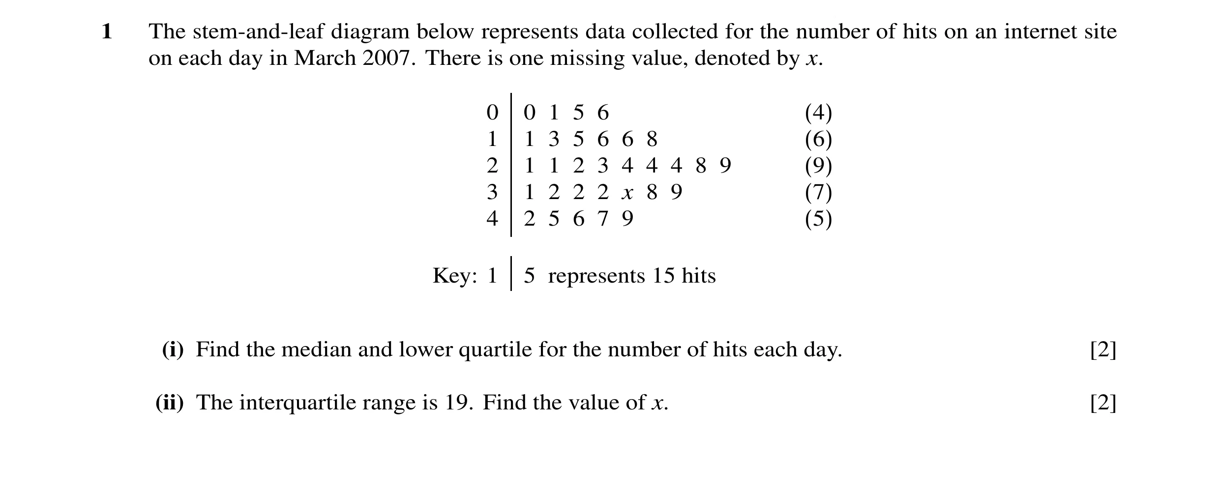
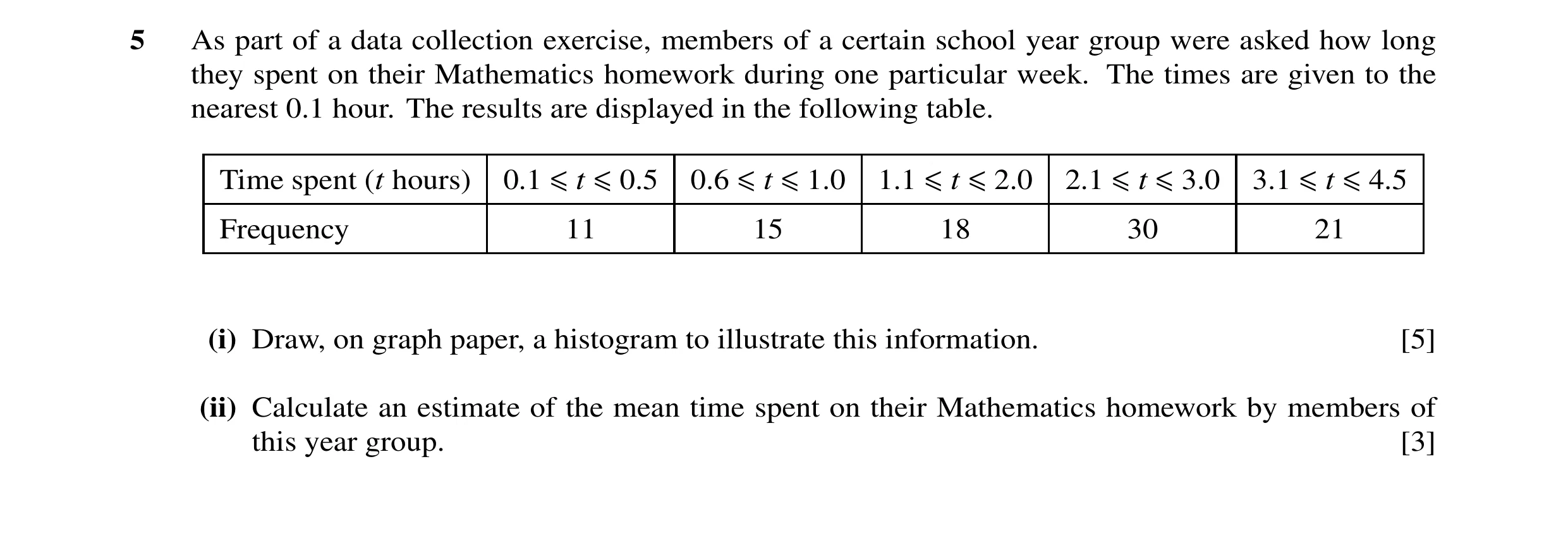

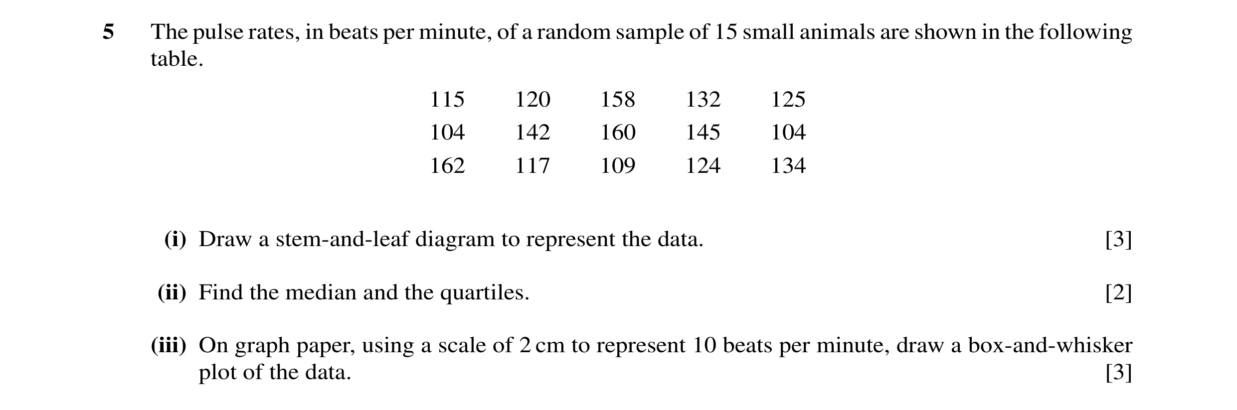 1 / 86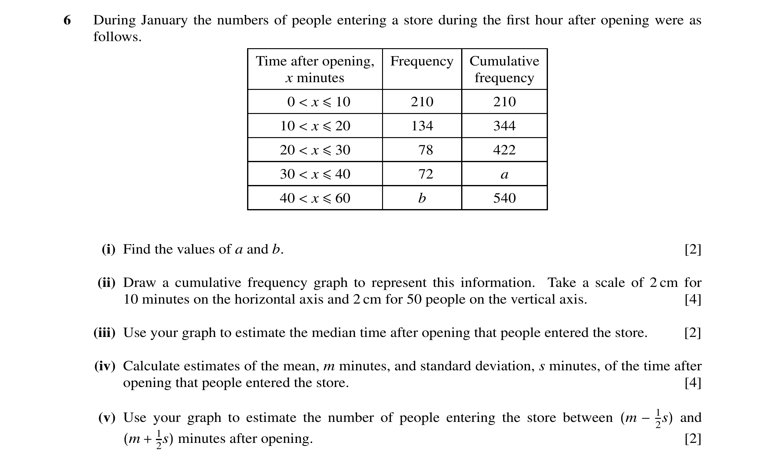
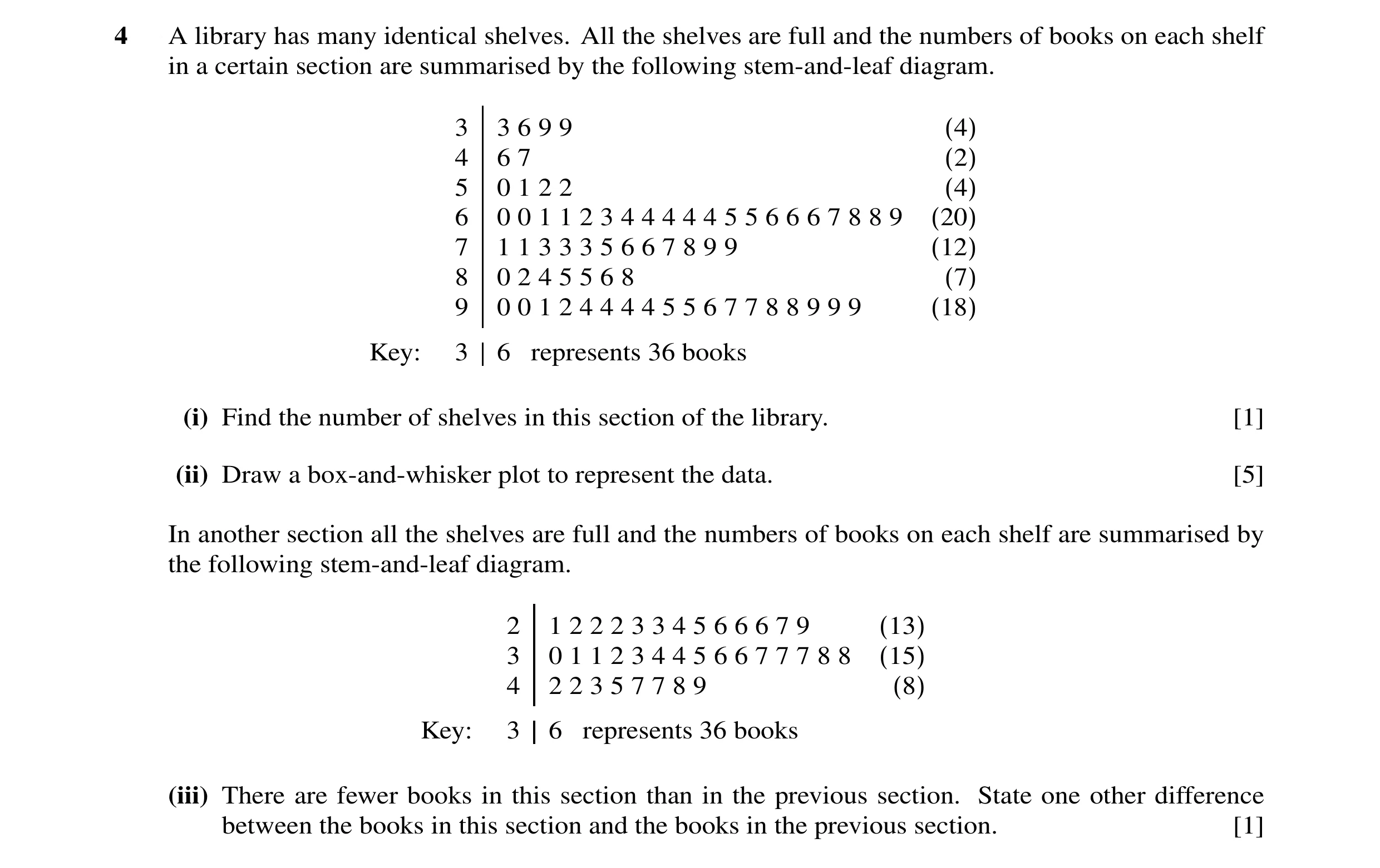 2 / 86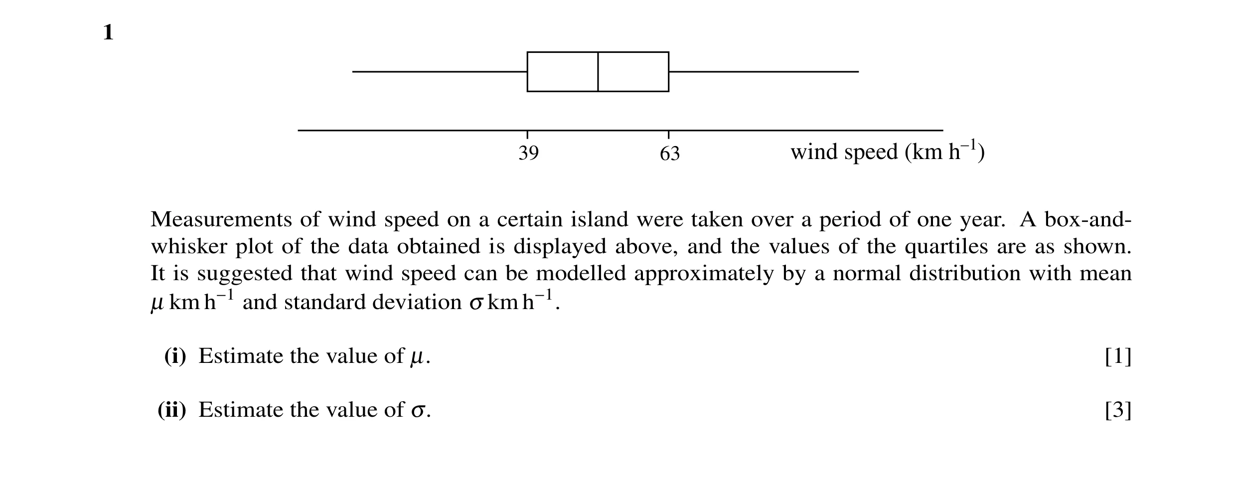
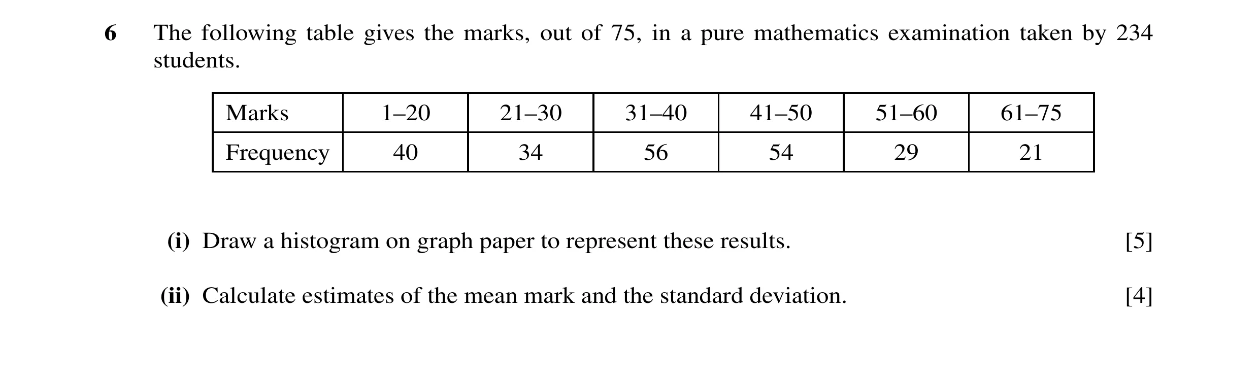
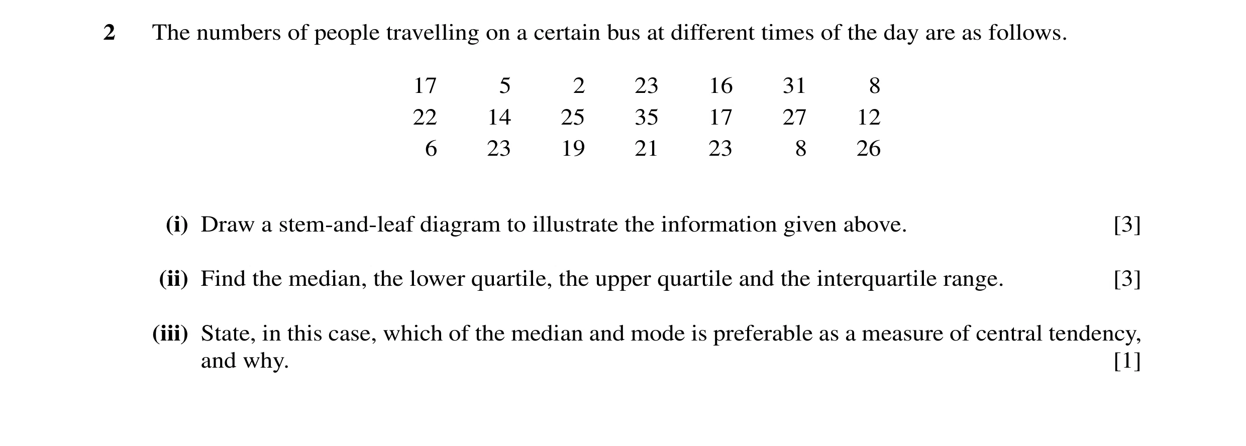 3 / 86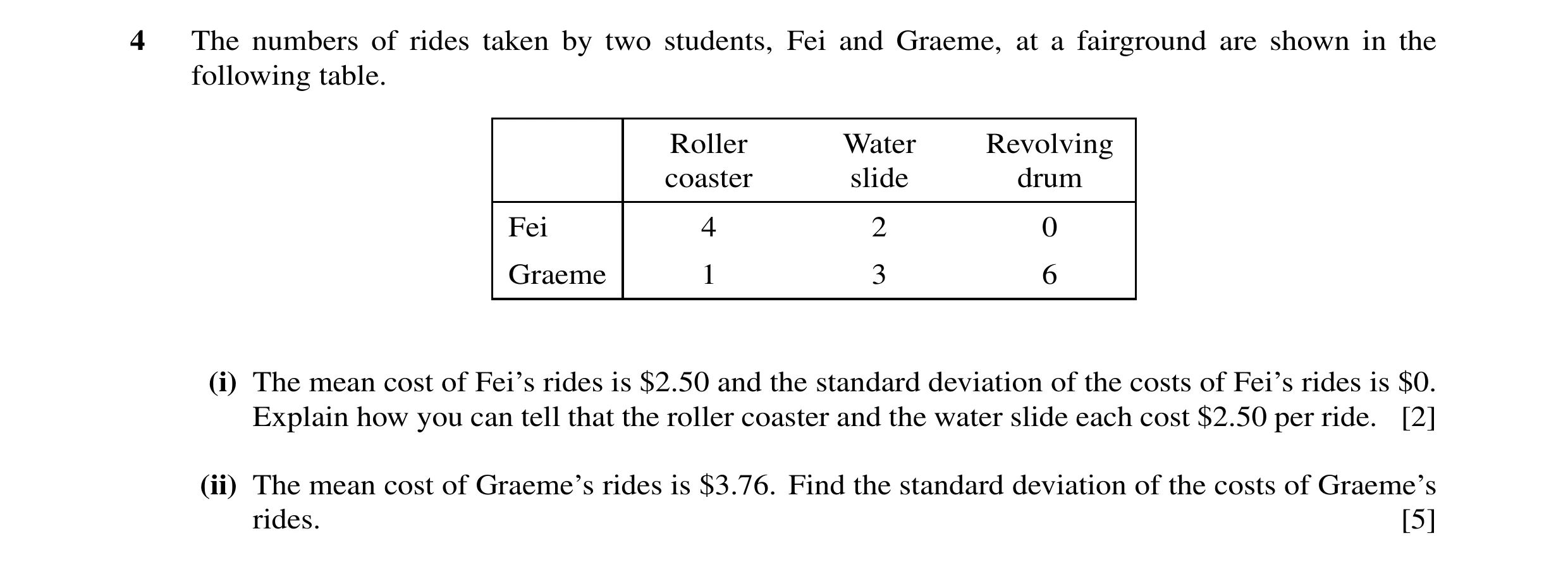
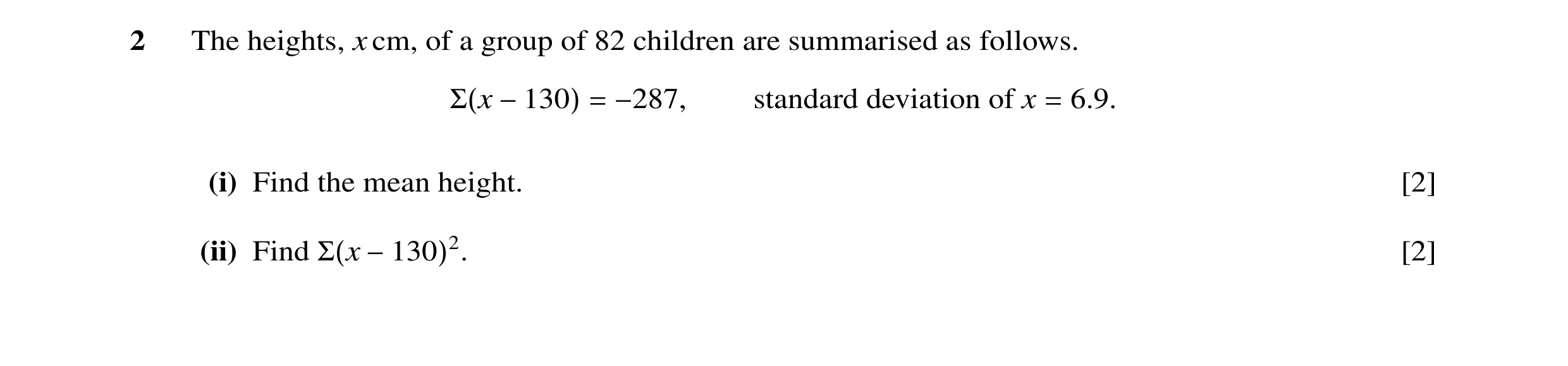
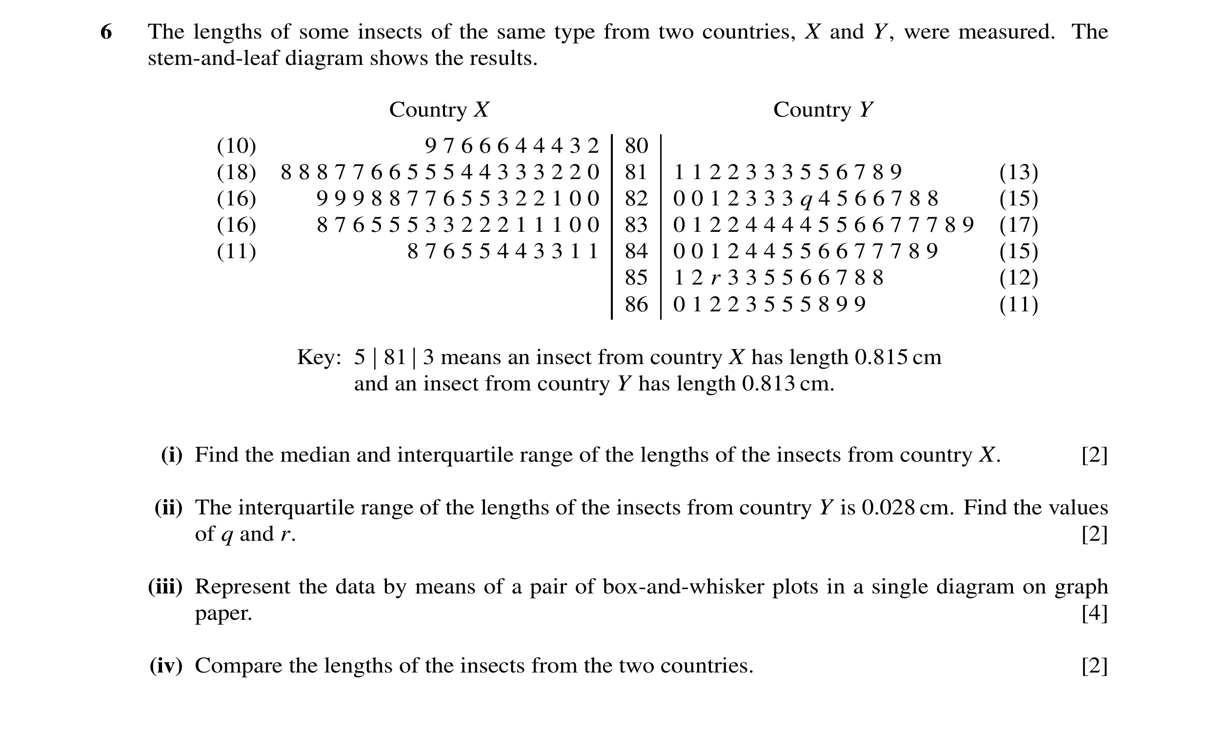 4 / 86
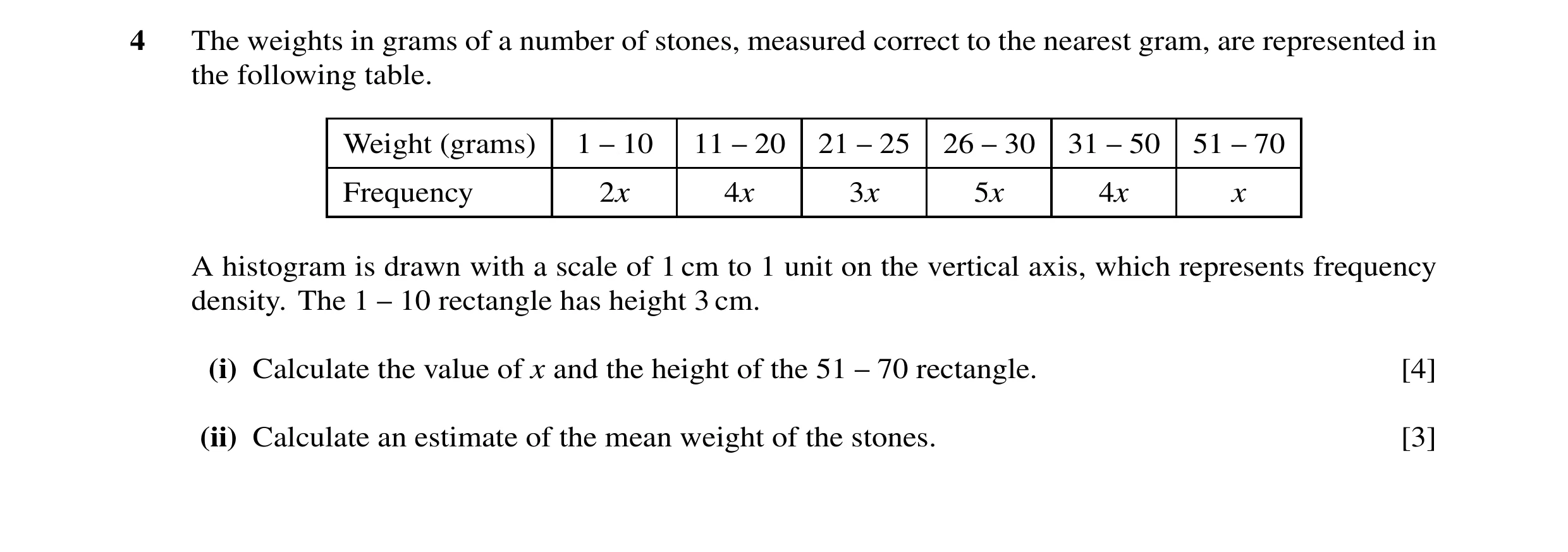
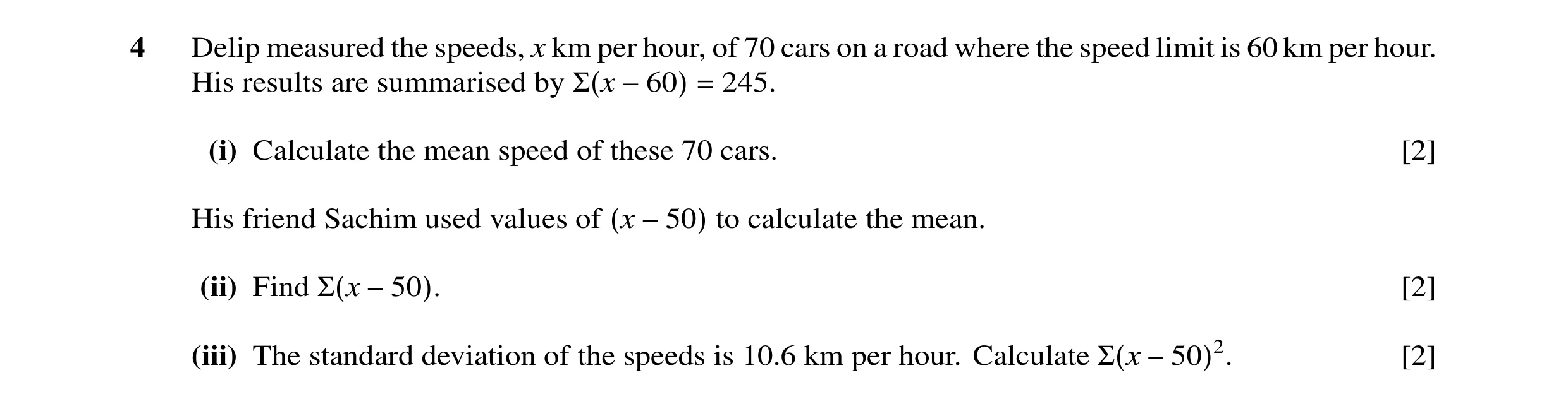 5 / 86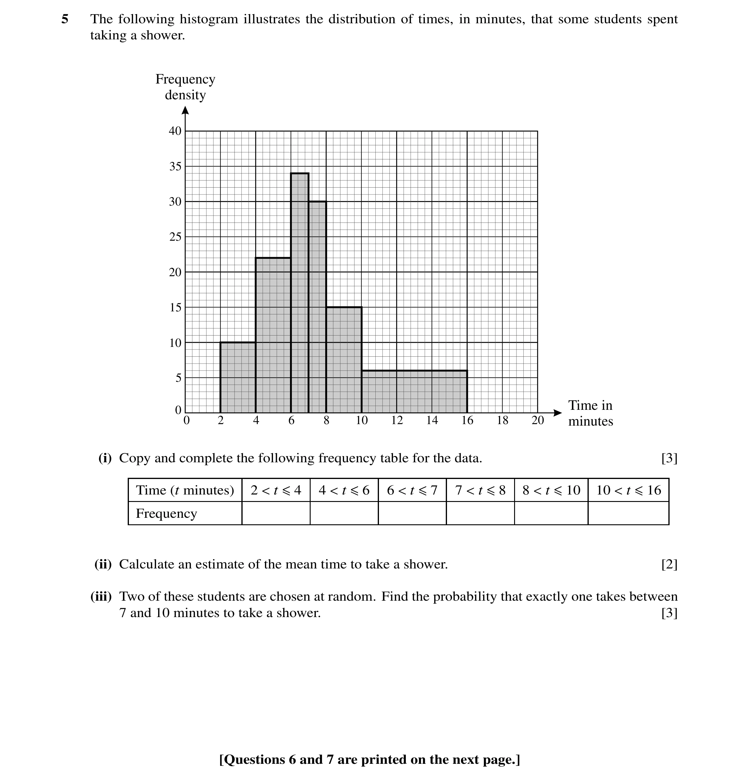
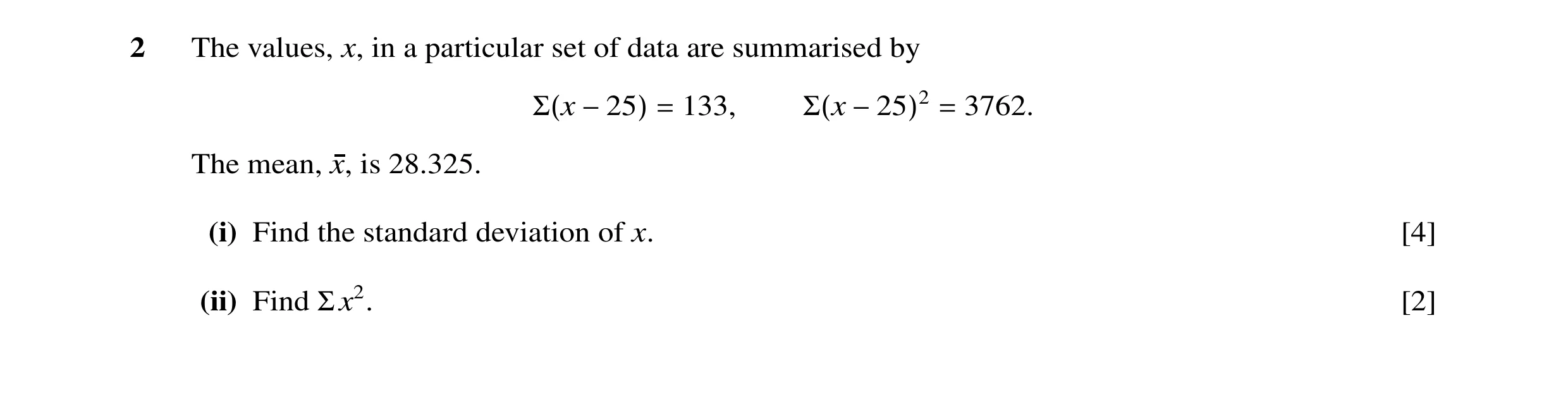 6 / 86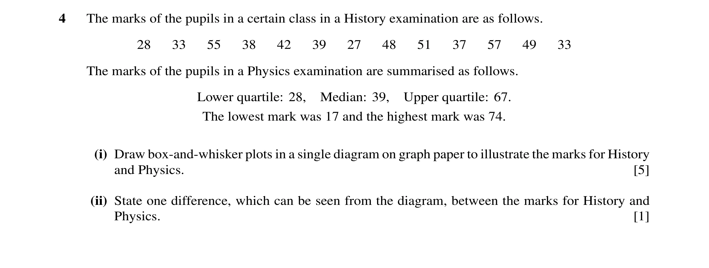

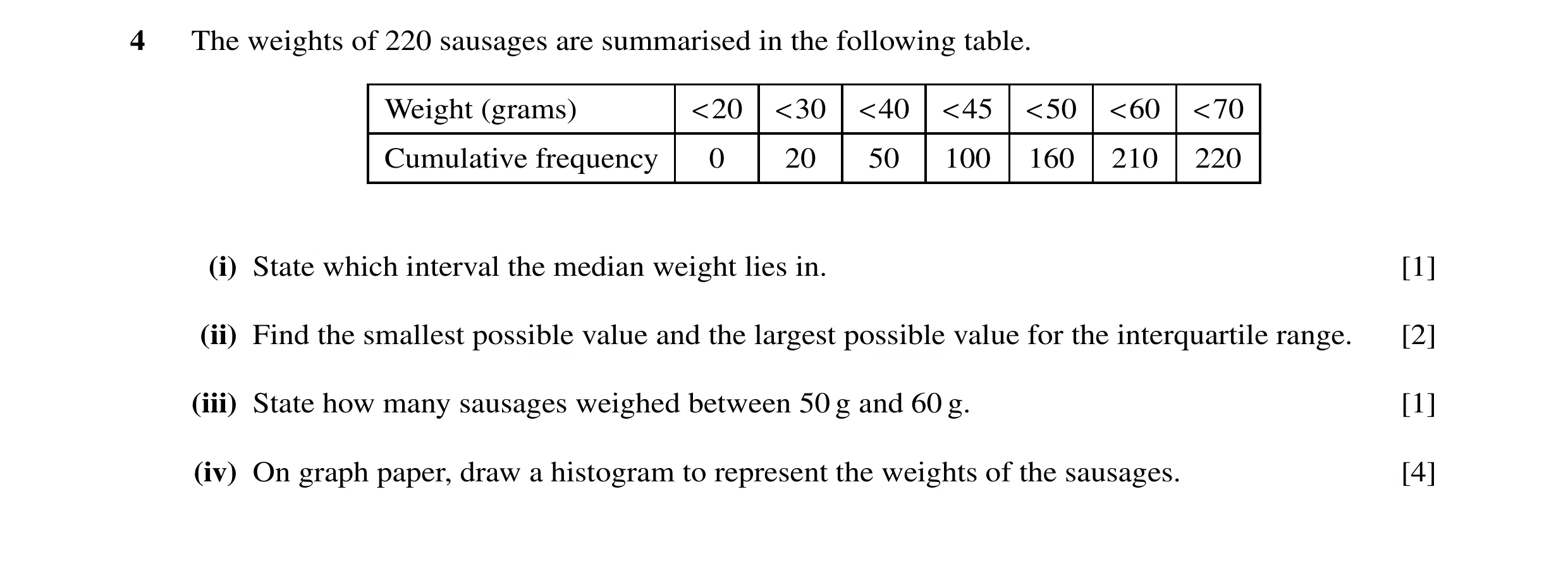 7 / 86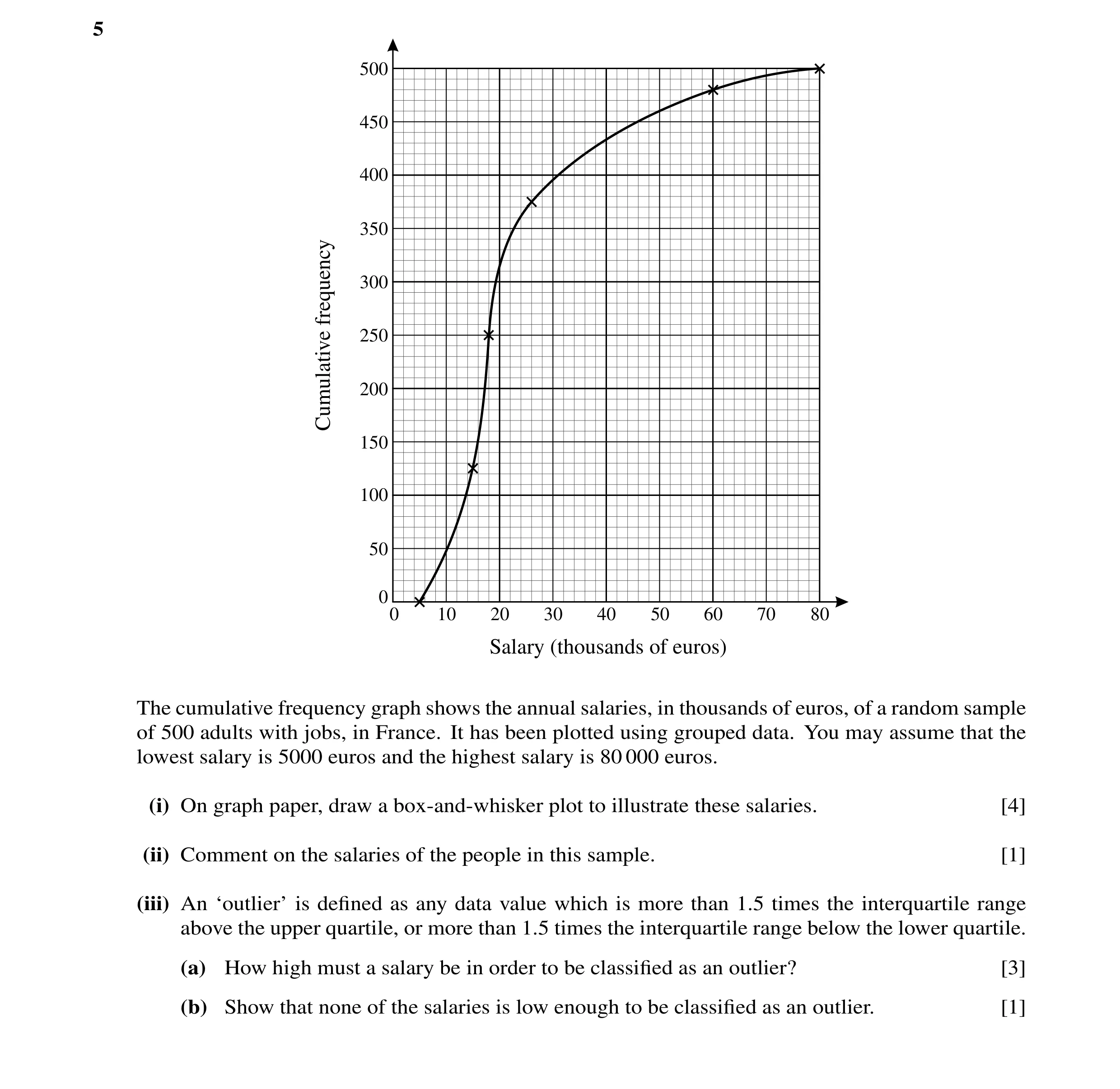
![Question 22: The ages, x years, of 150 cars are summarised by Σx = 645 and Σ x2 = 8287.5. Find Σ(x −x)2, where x denotes the mean of x. [4]](https://img.pastlit.com/crops/bb1f146d-021e-46d7-b5a7-8d2ede2b337a/q1.webp) 8 / 86
8 / 86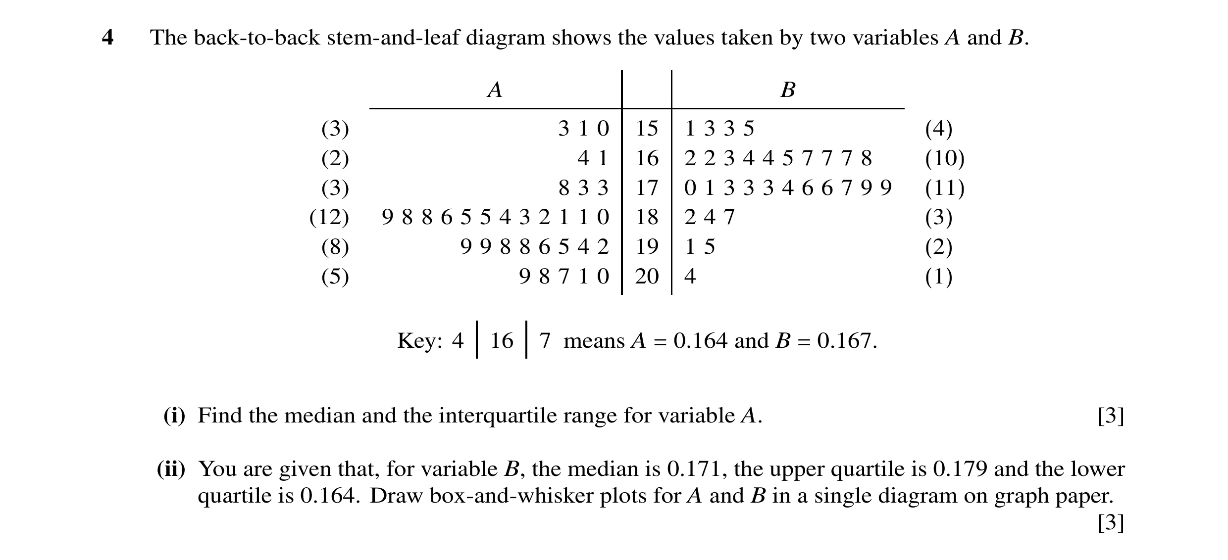
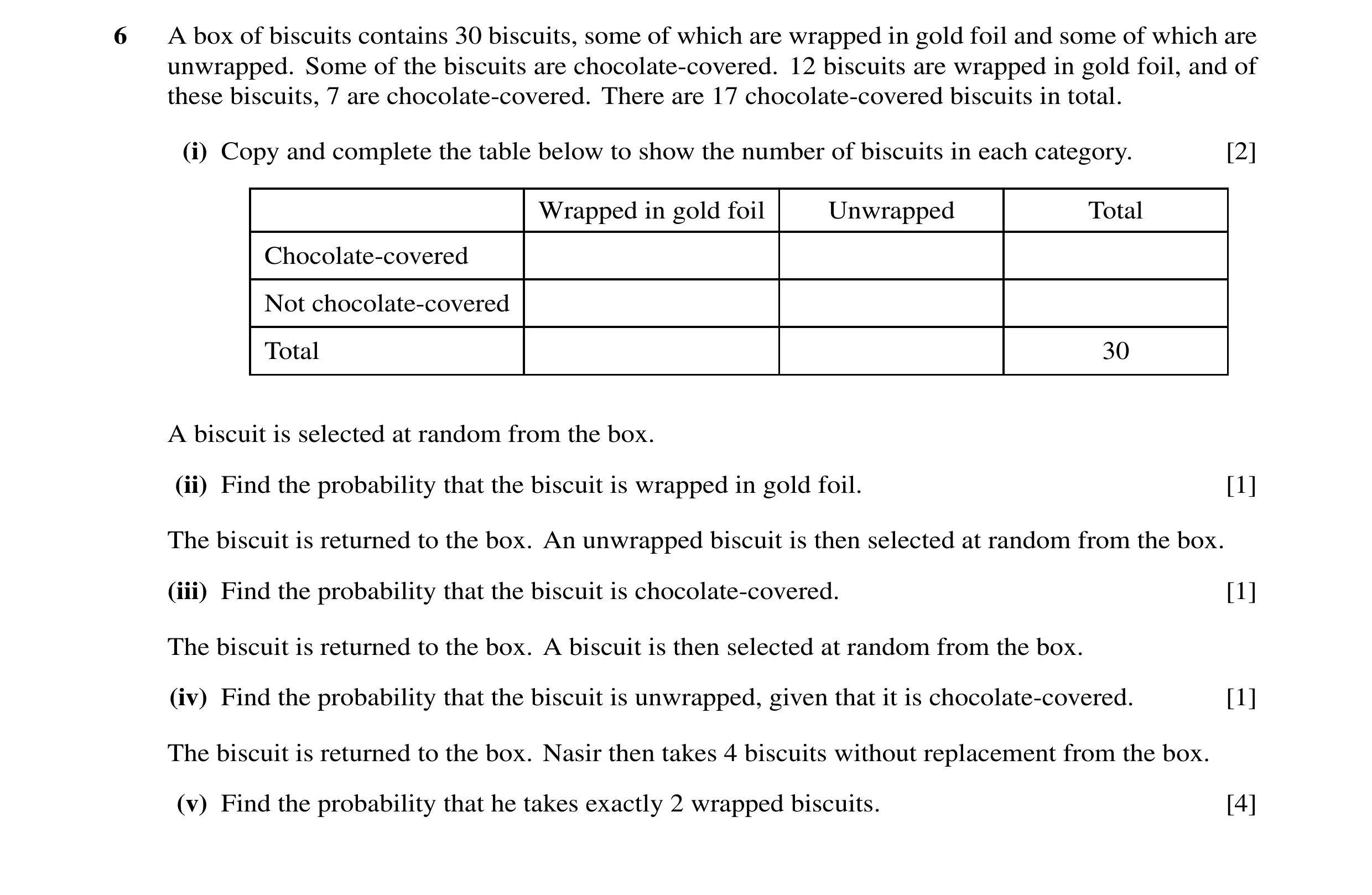
 9 / 86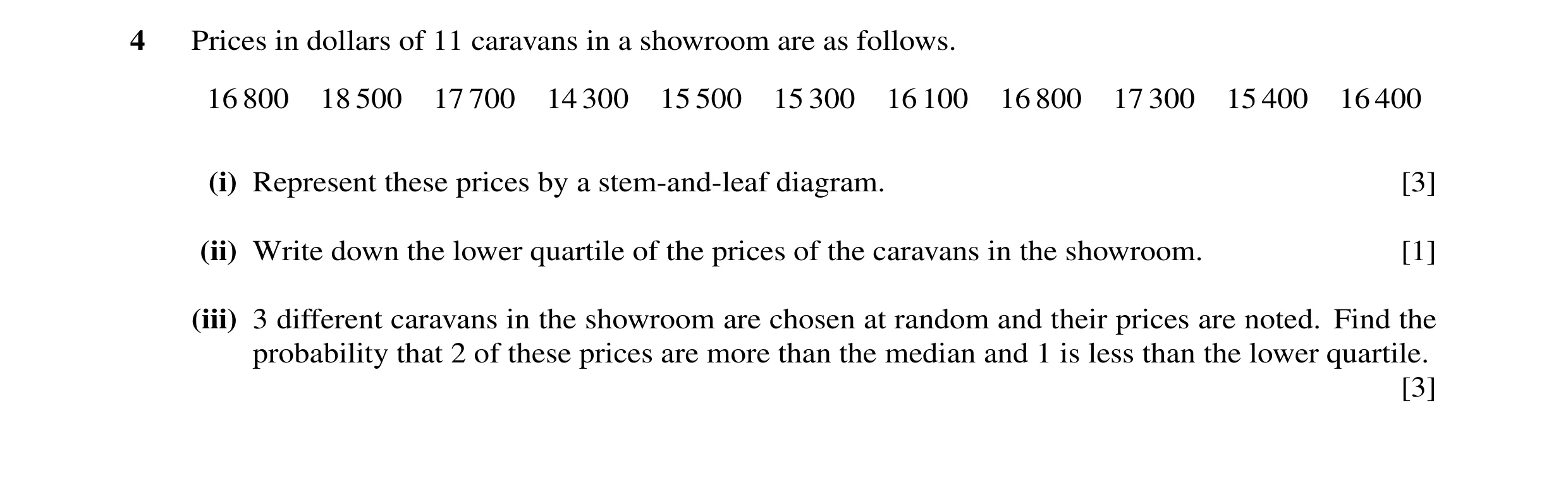
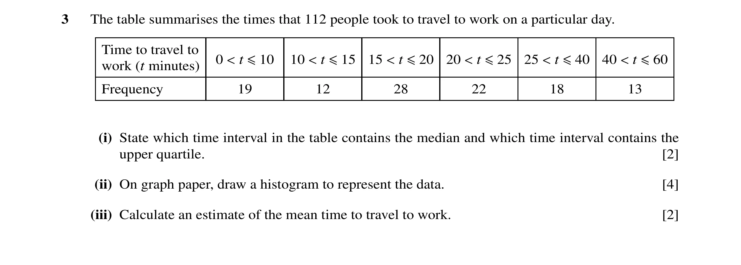
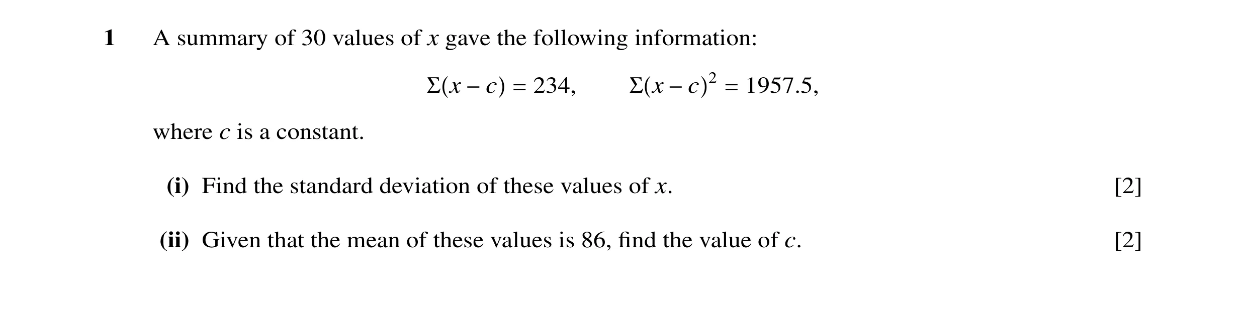 10 / 86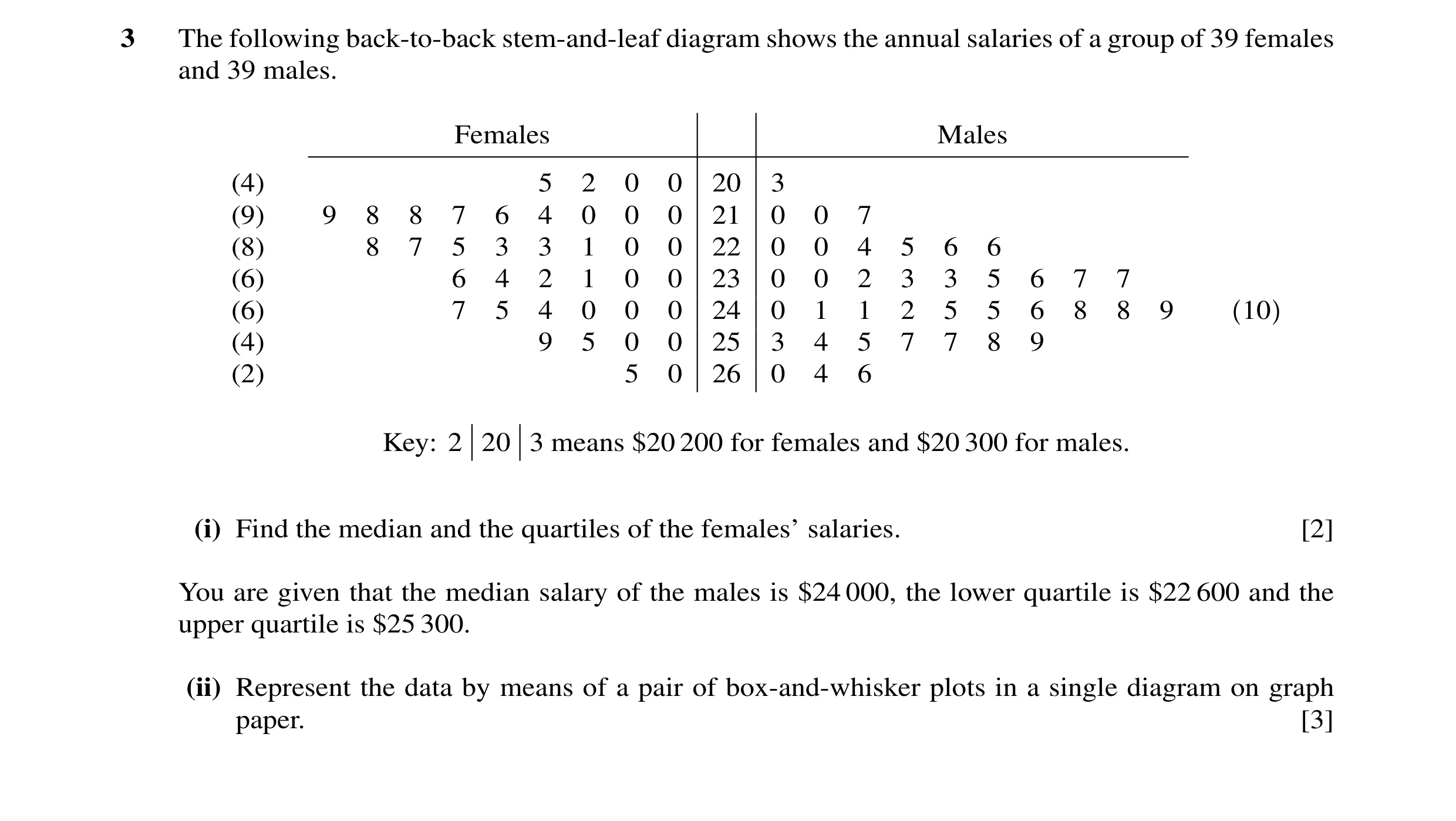

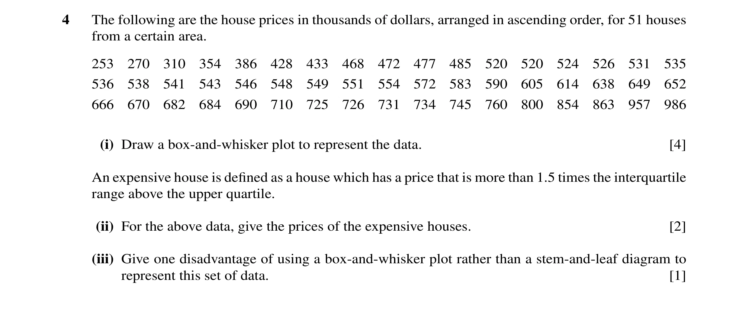 11 / 86
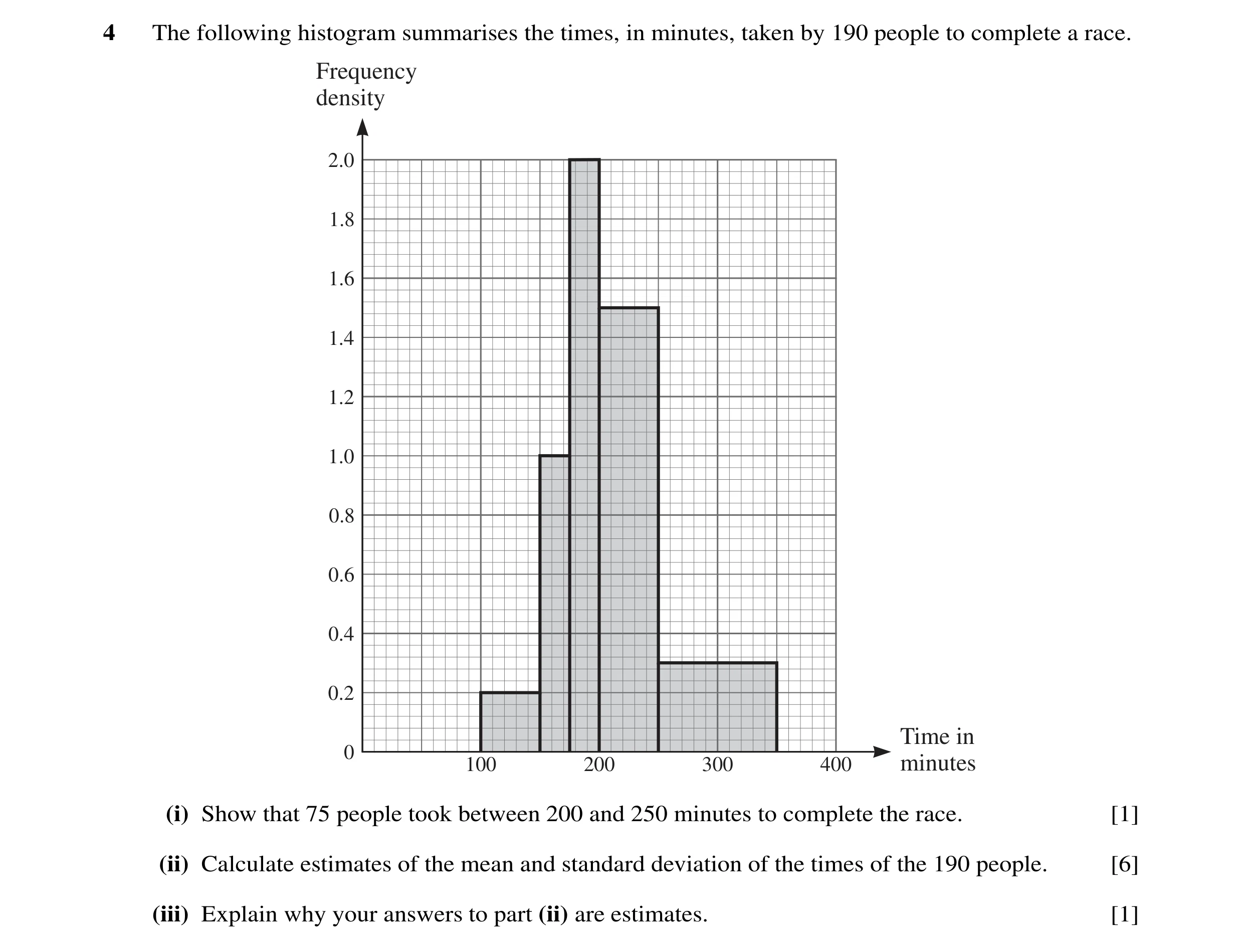 12 / 86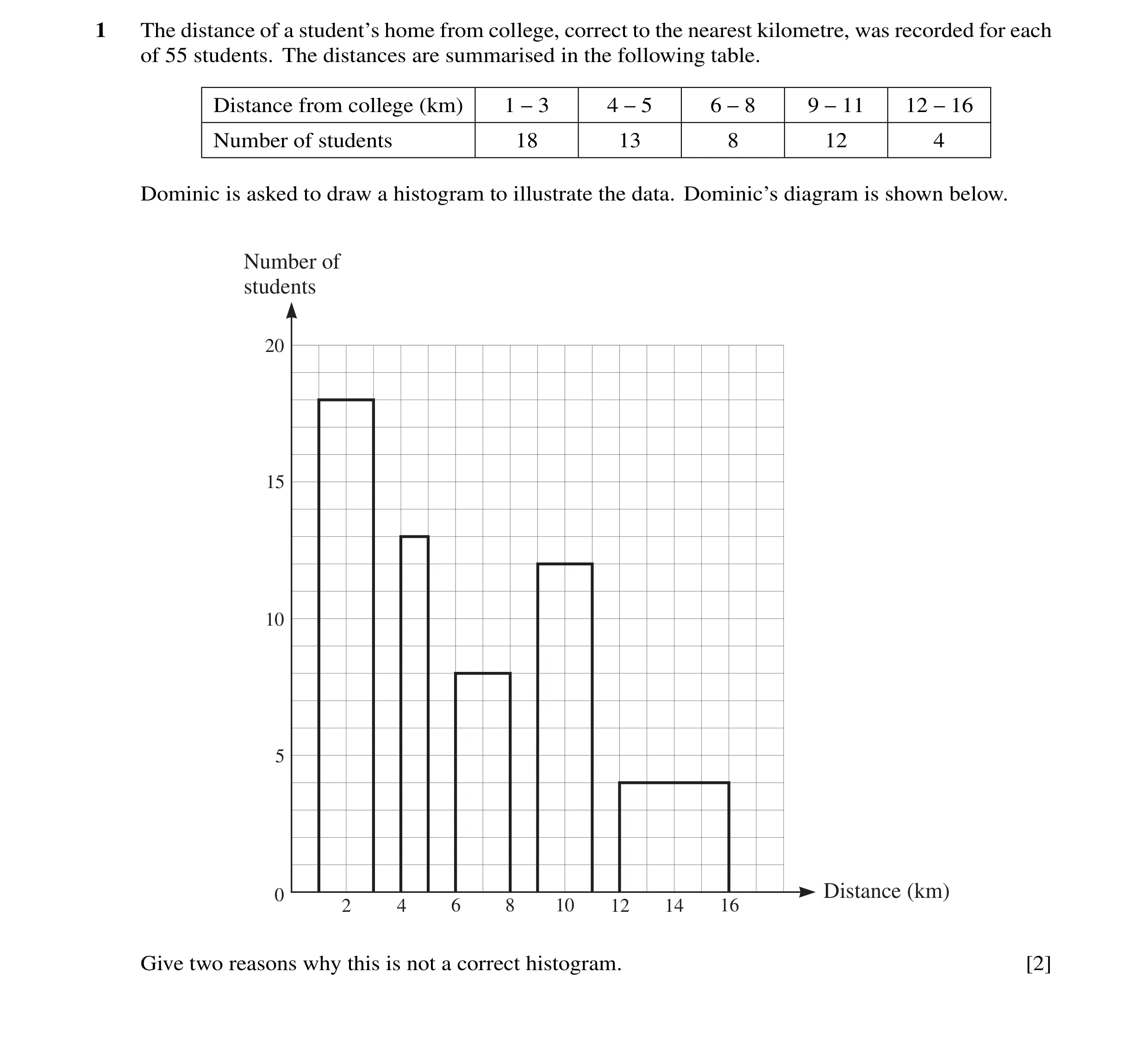
 13 / 86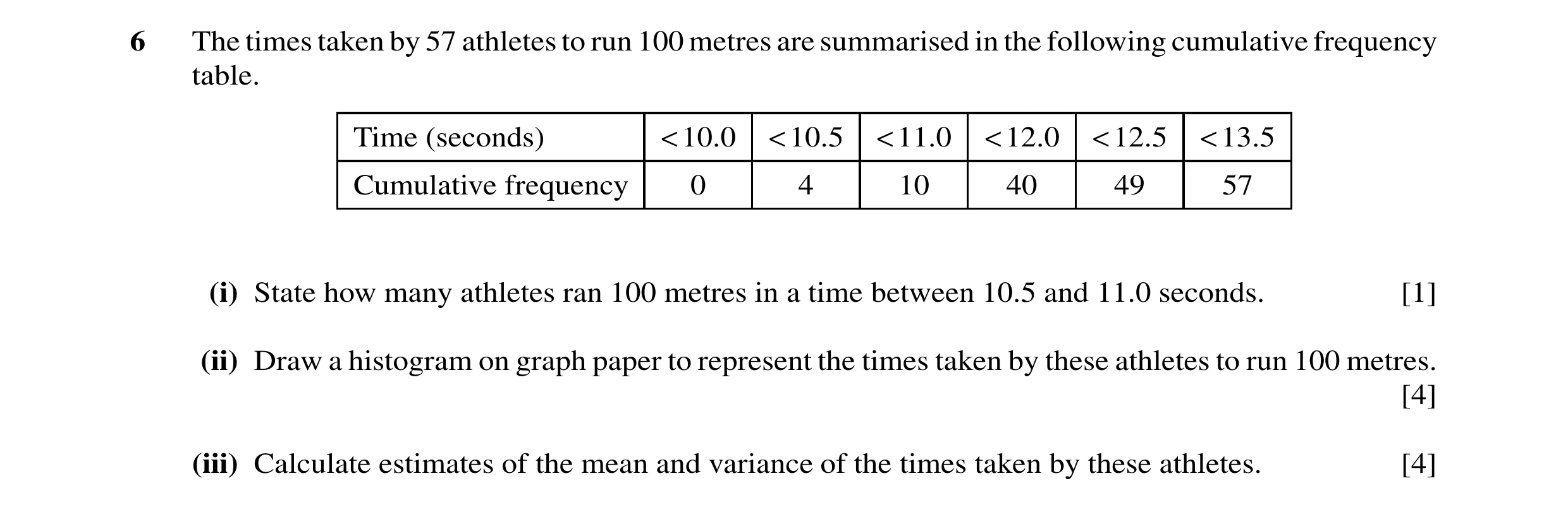
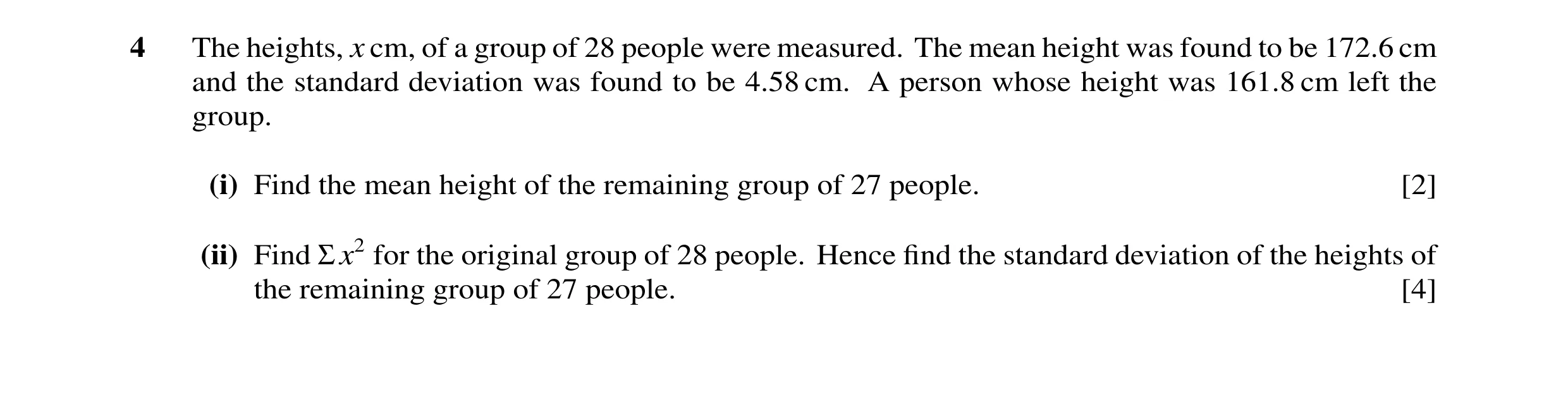
![Question 37: Find the mean and variance of the following data. [3] 5 −2 12 7 −3 2 −6 4 0 8](https://img.pastlit.com/crops/7608a28f-37be-436a-a9b0-8a48a3e0f2a1/q1.webp)
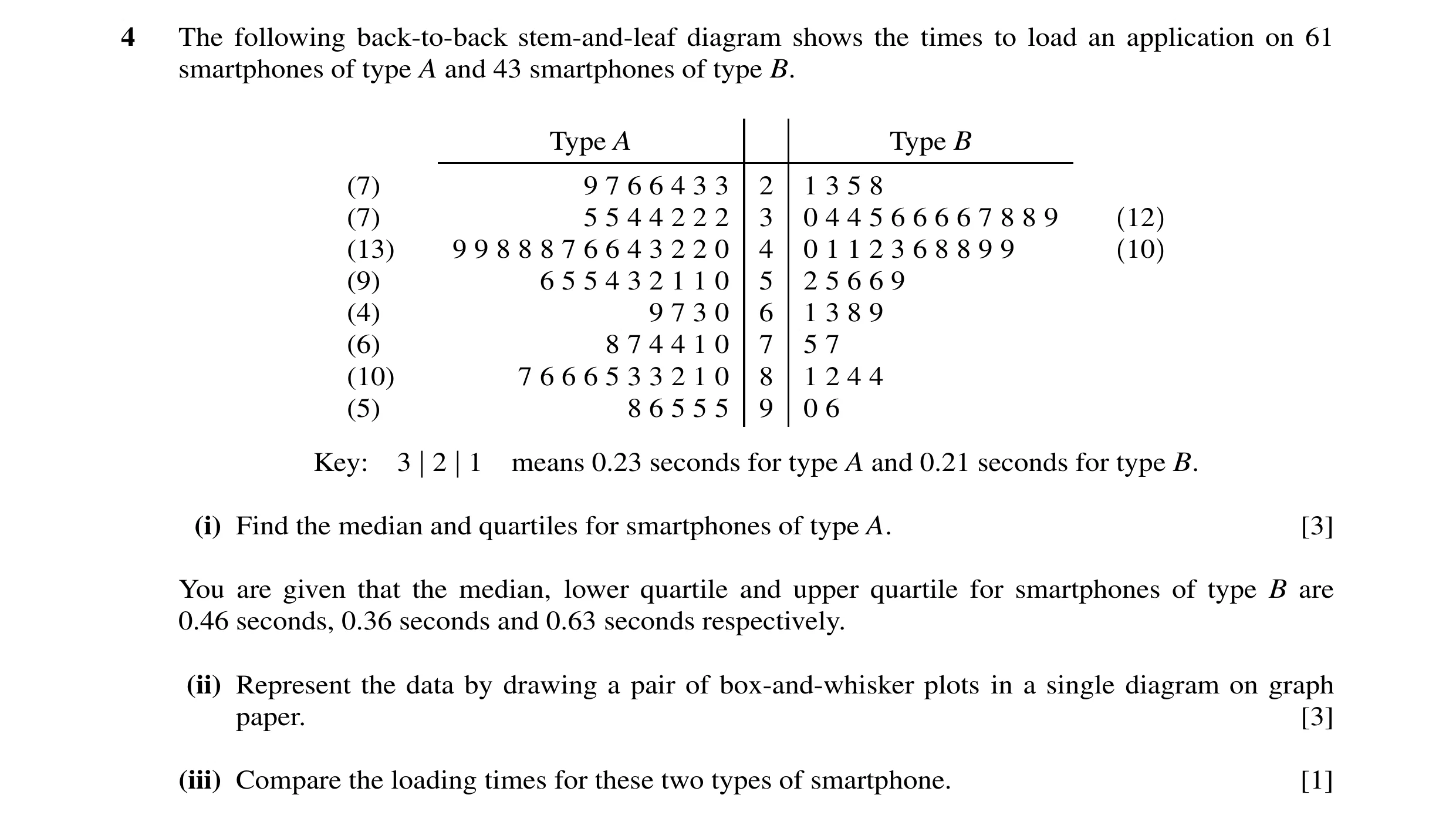 14 / 86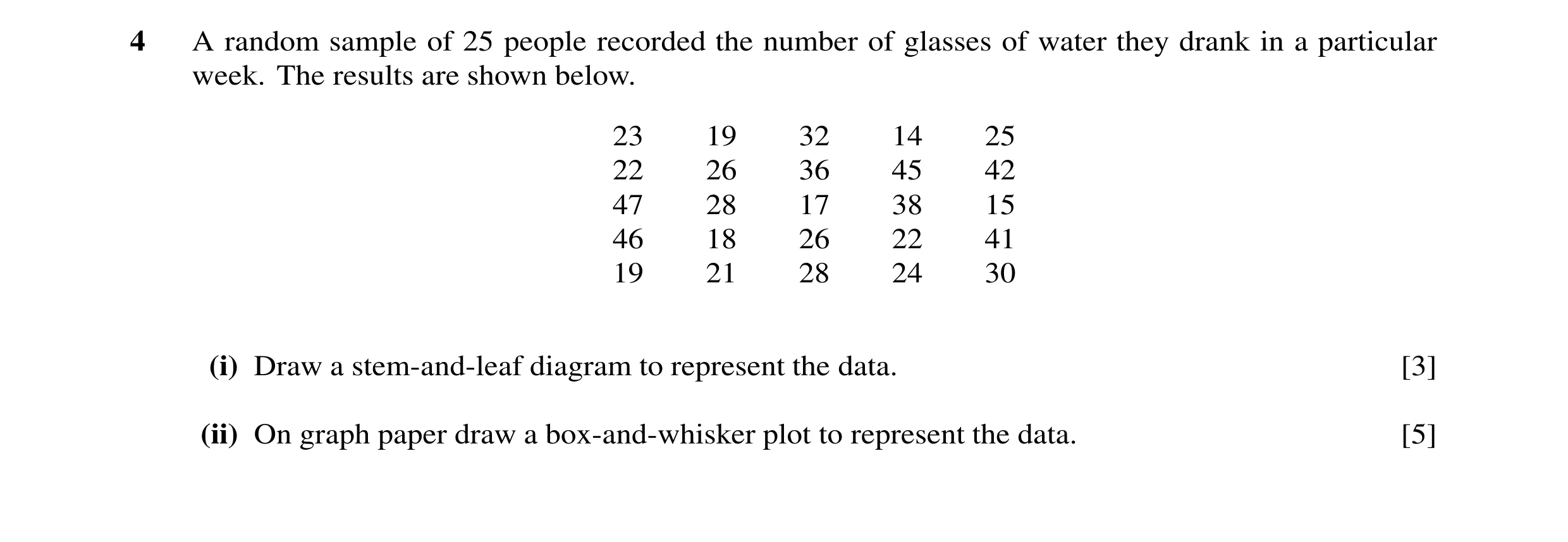
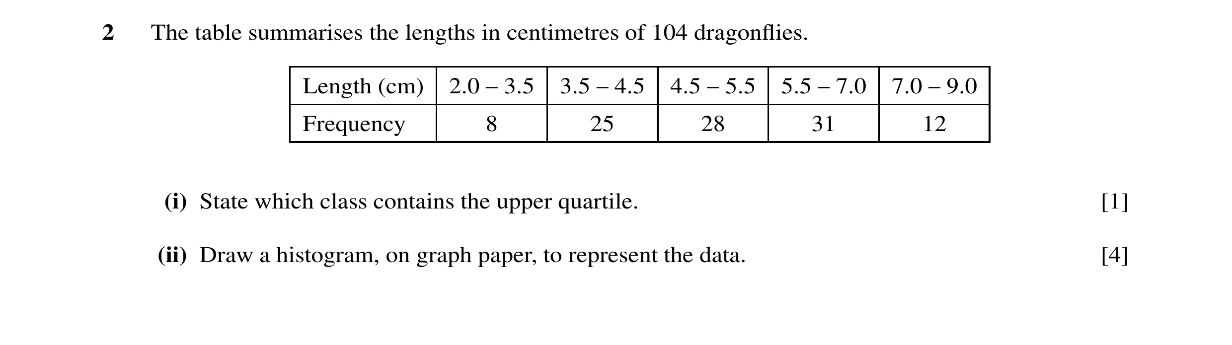
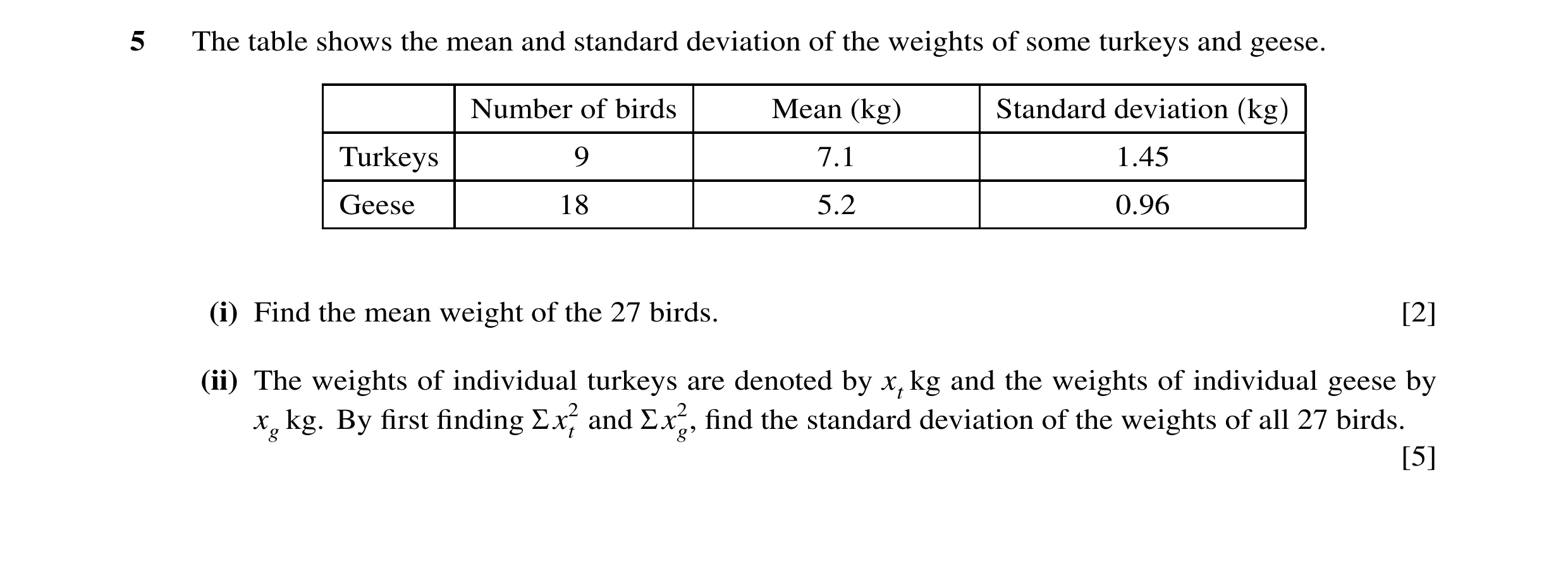 15 / 86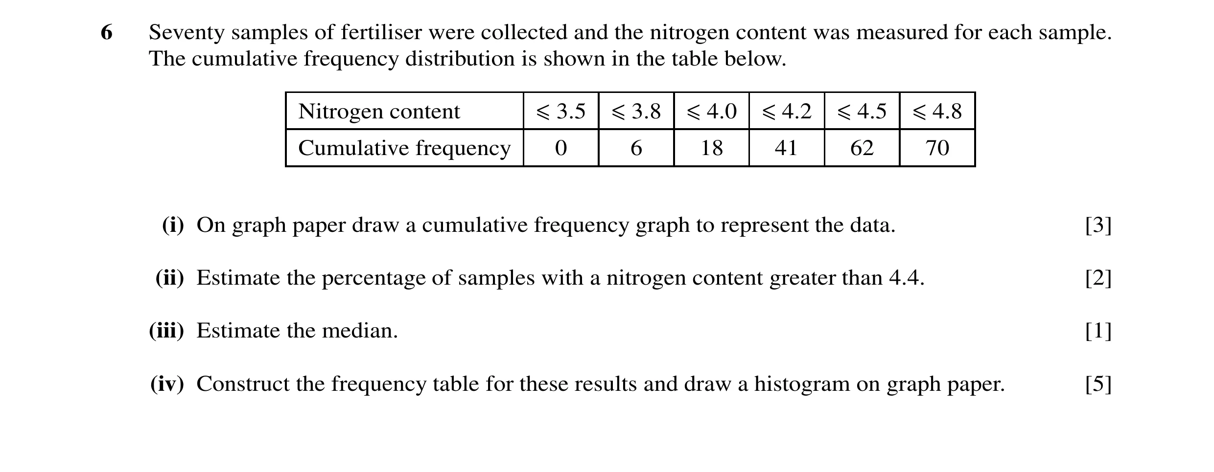
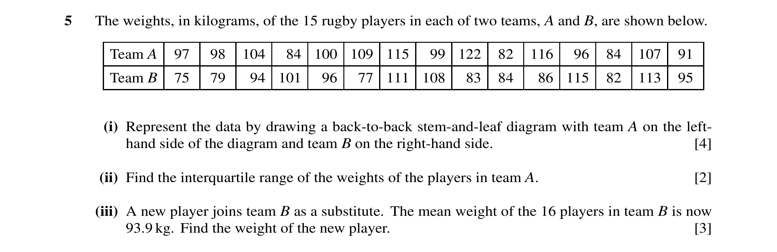
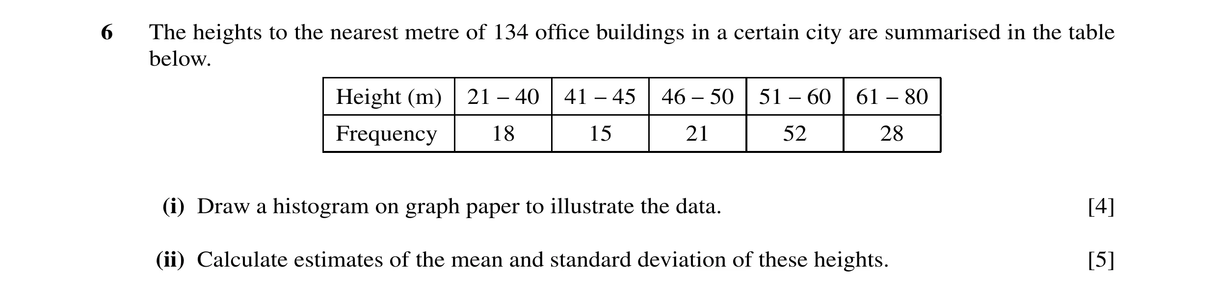
![Question 45: For 10 values of x the mean is 86.2 and Σ x −a = 362. Find the value of (i) Σx, [1] (ii) the constant a. [2]](https://img.pastlit.com/crops/e5a507aa-a734-4fc6-885b-2bc33bfd67d4/q1.webp) 16 / 86
16 / 86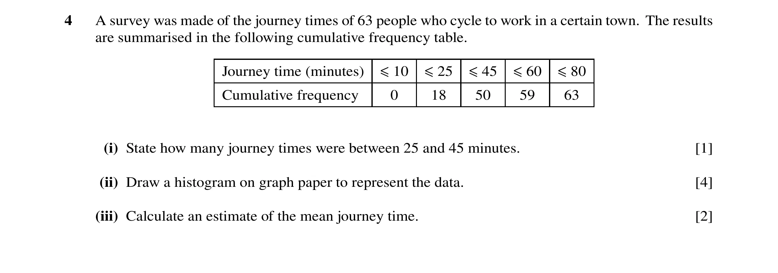
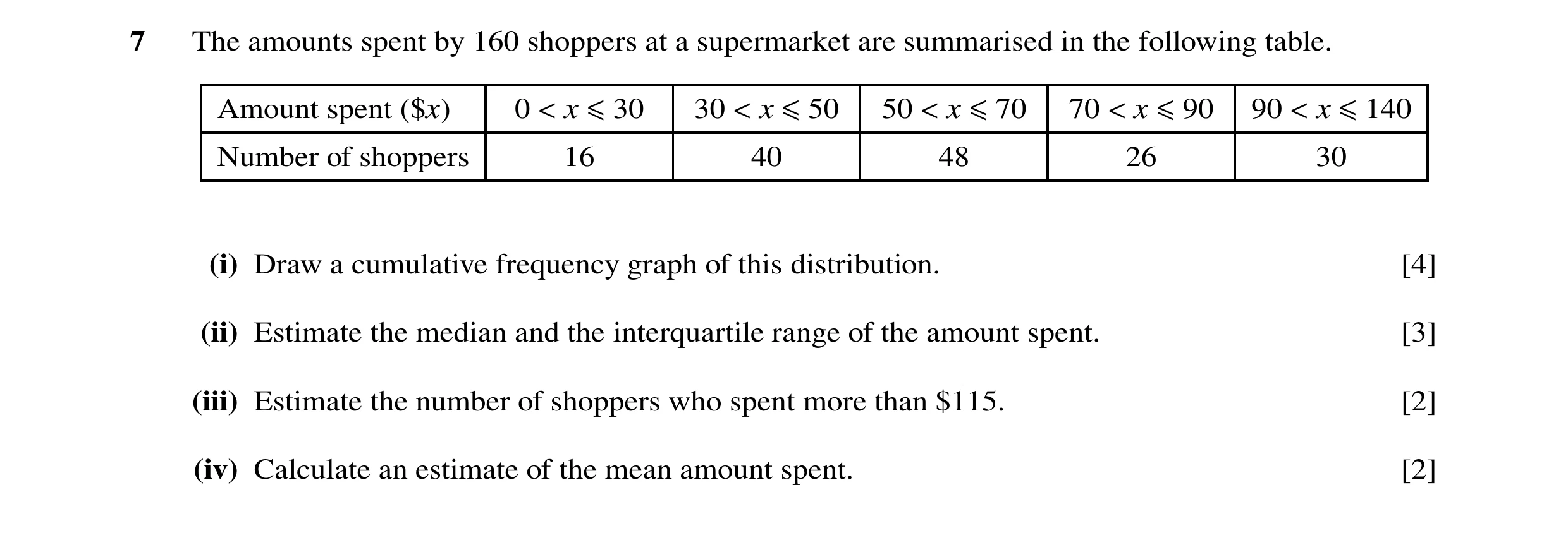
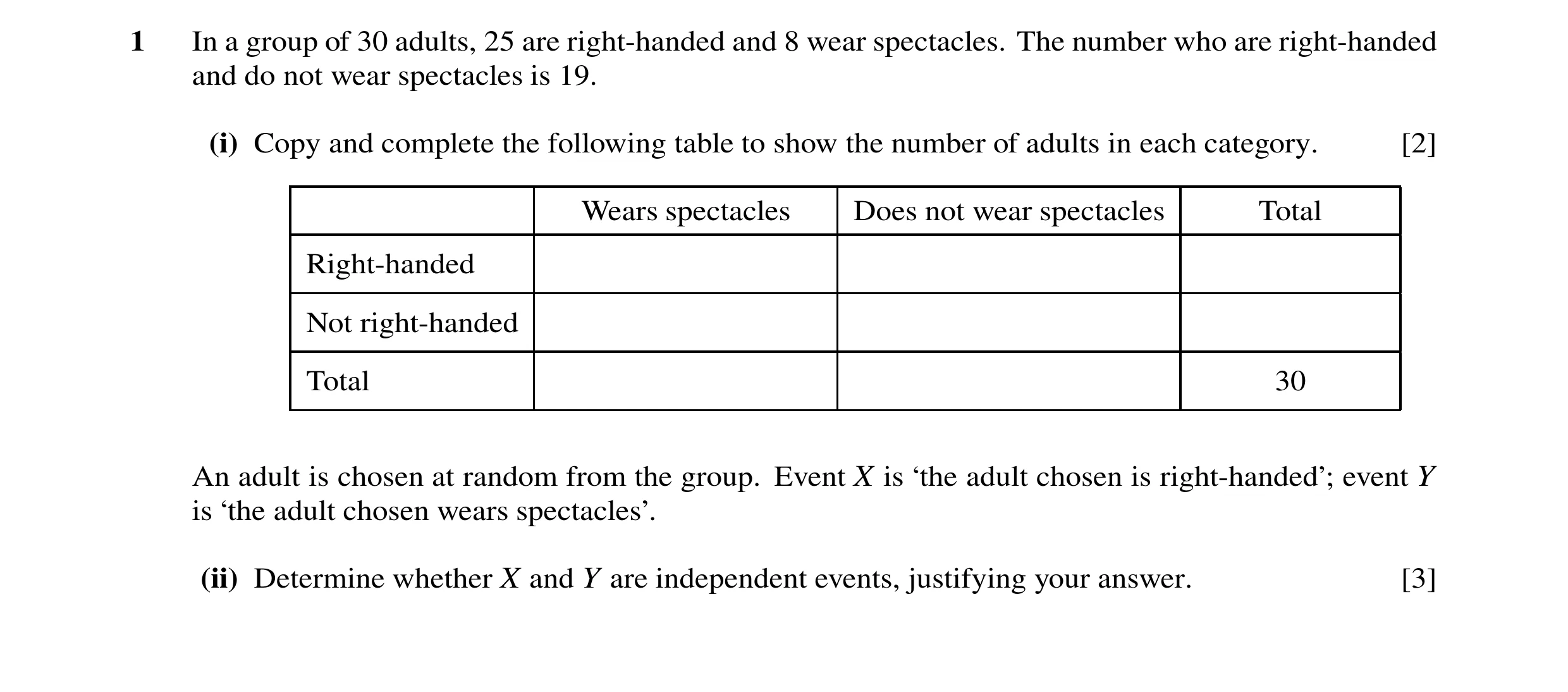 17 / 86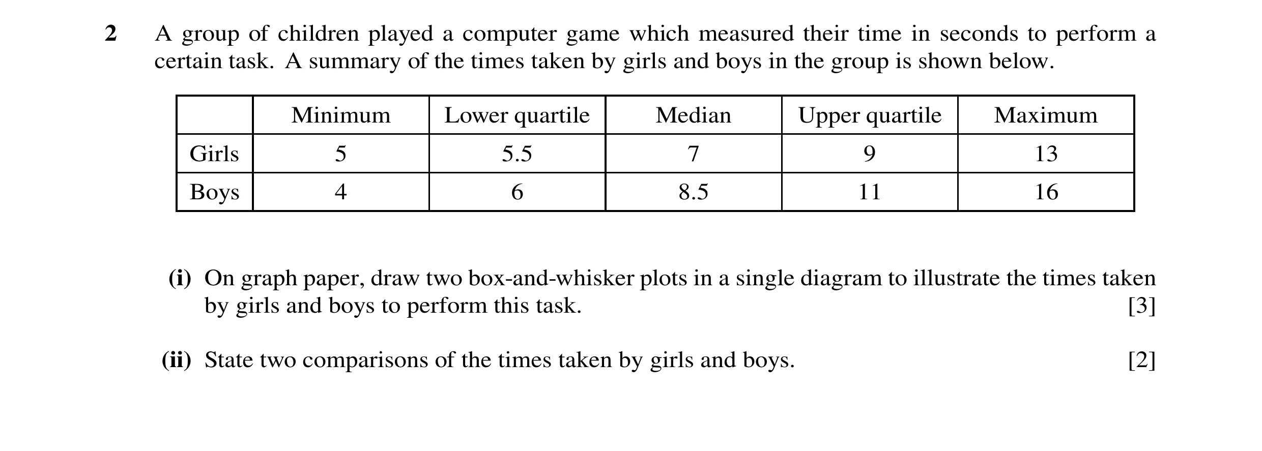
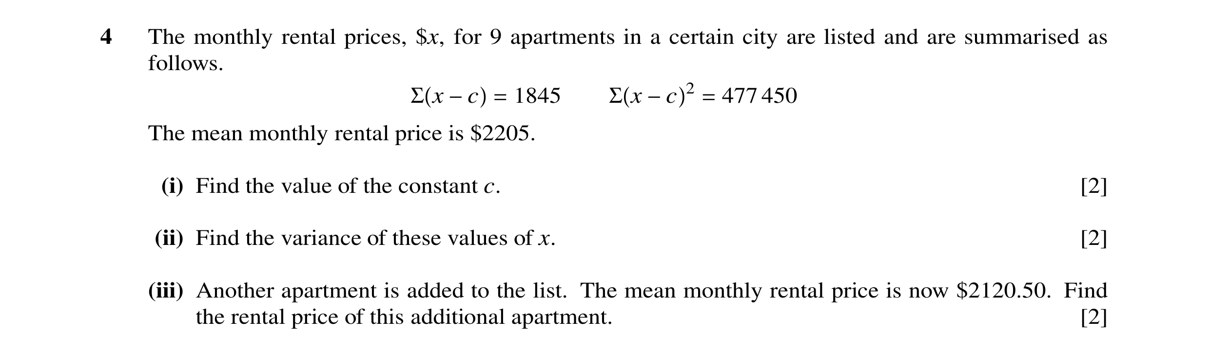
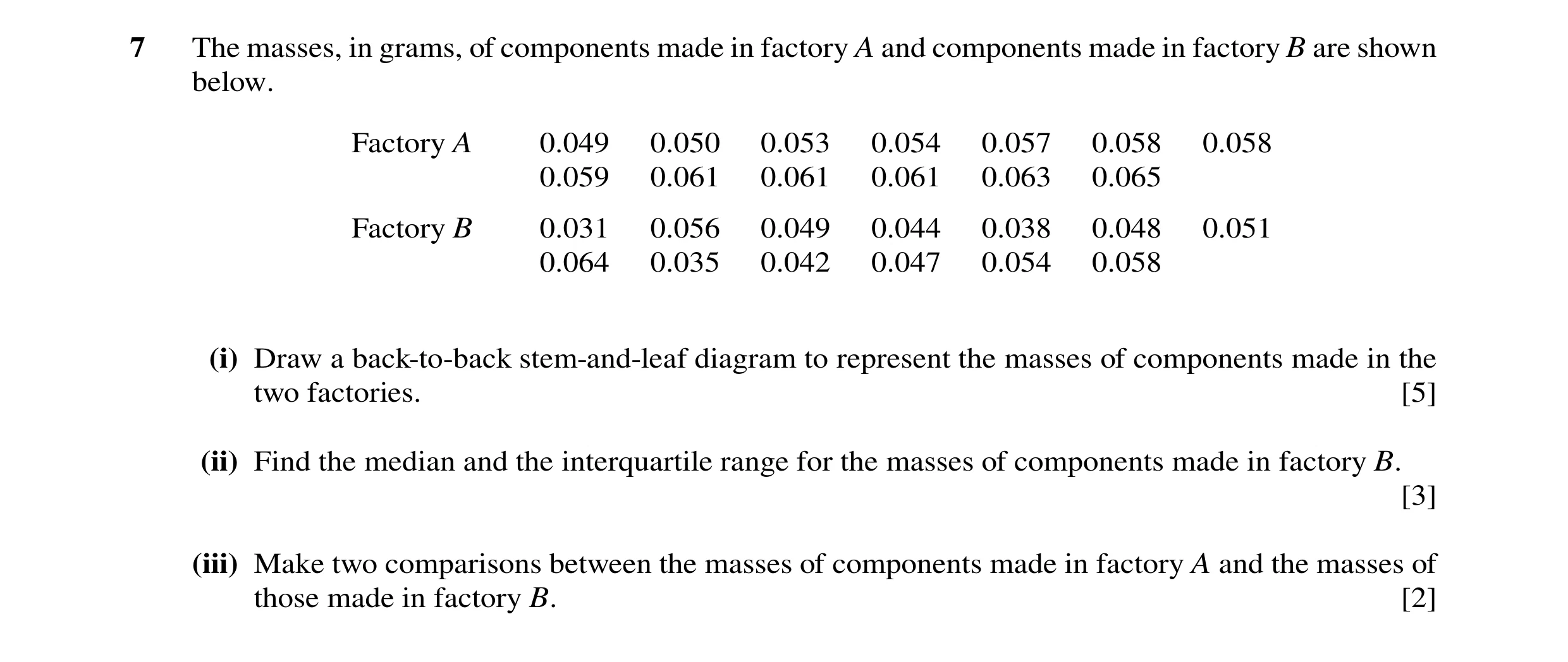 18 / 86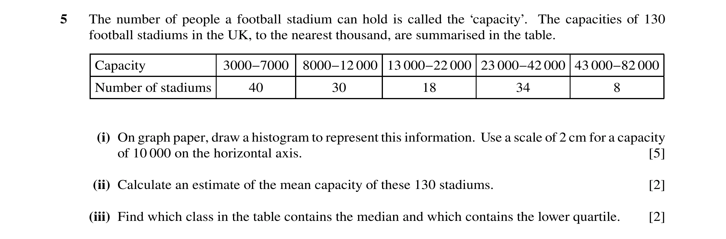
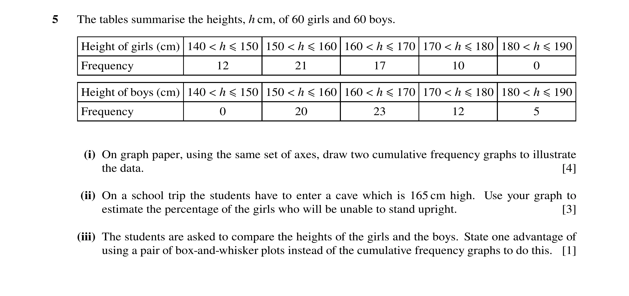 19 / 86
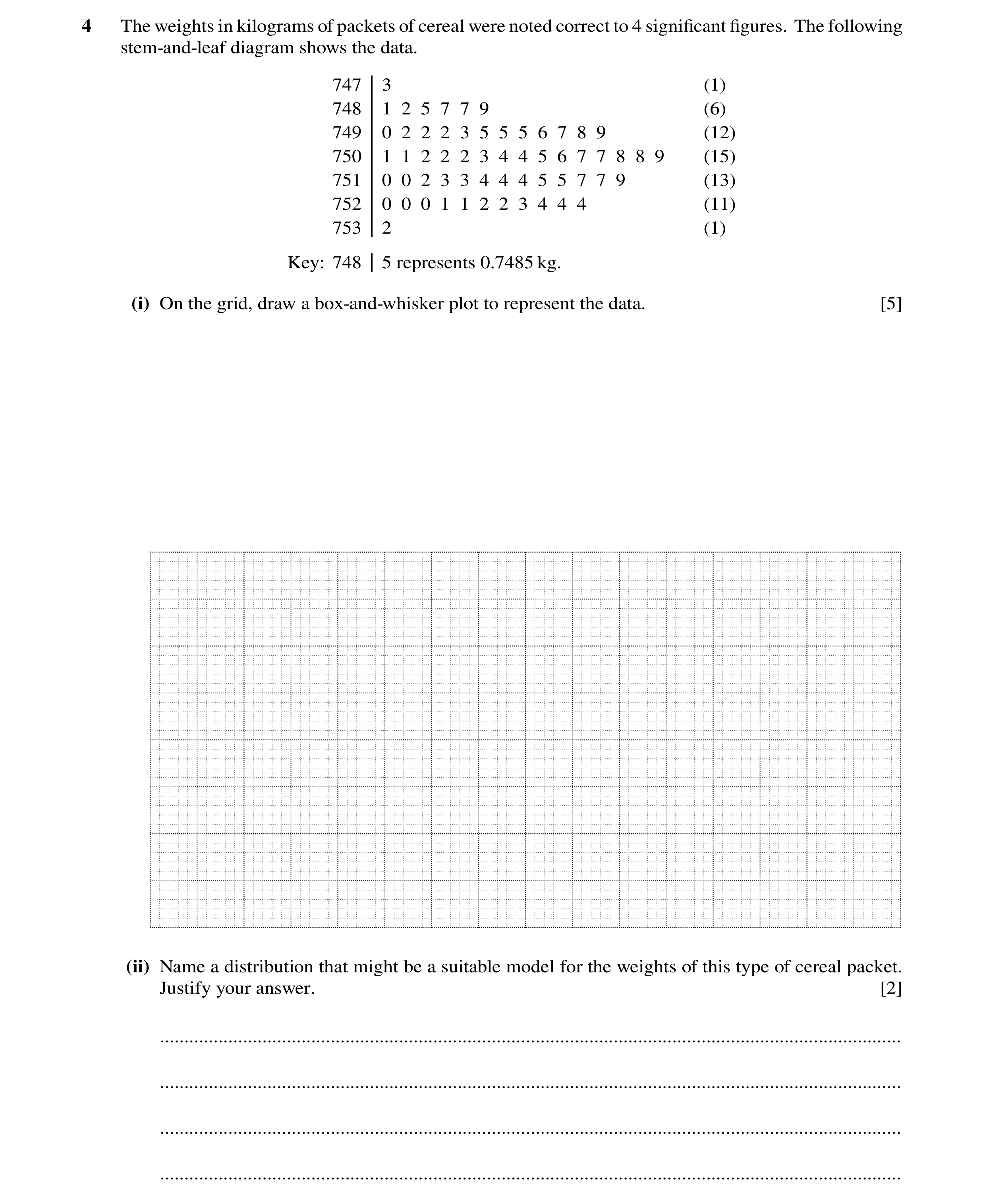 20 / 86
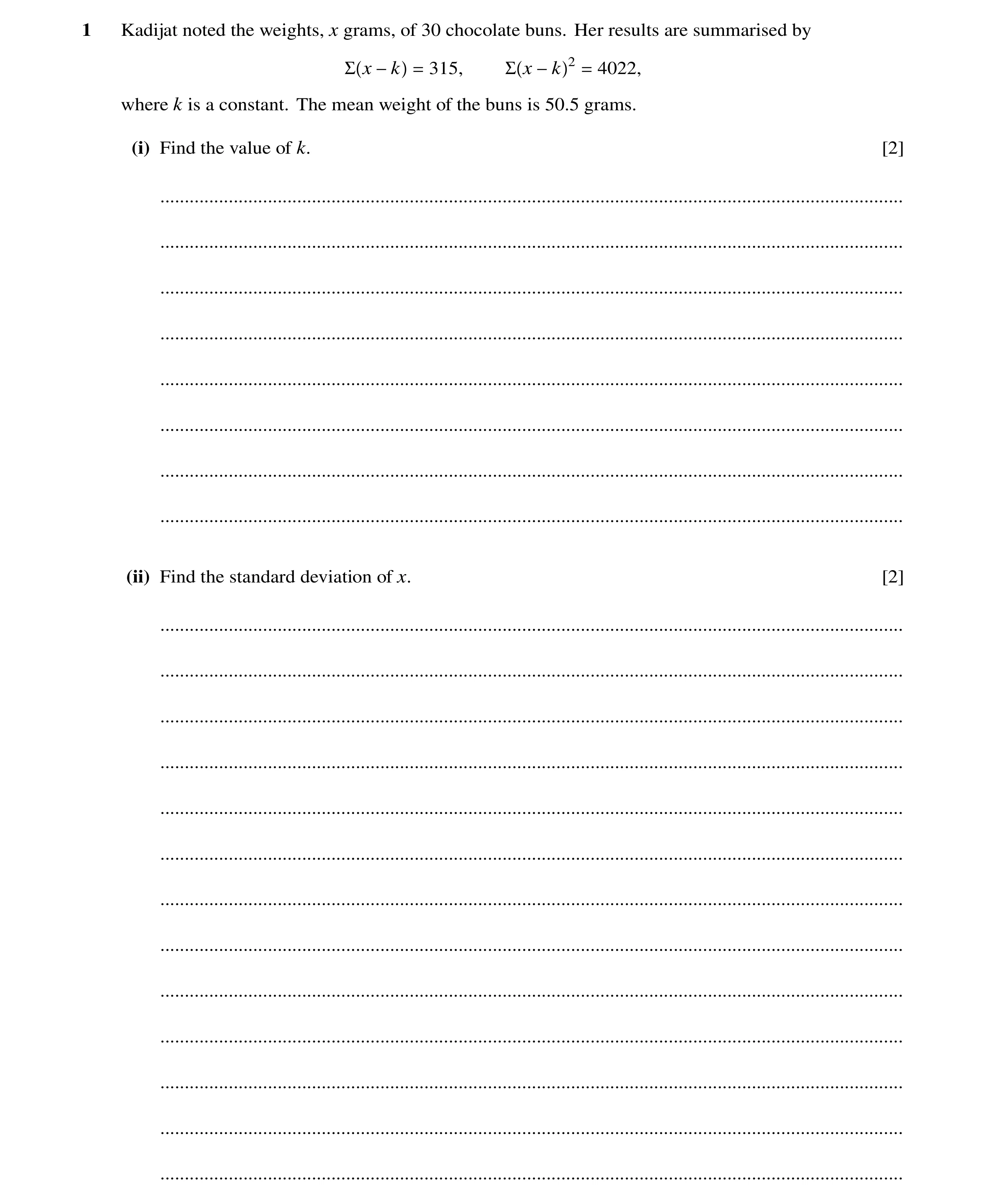 21 / 86
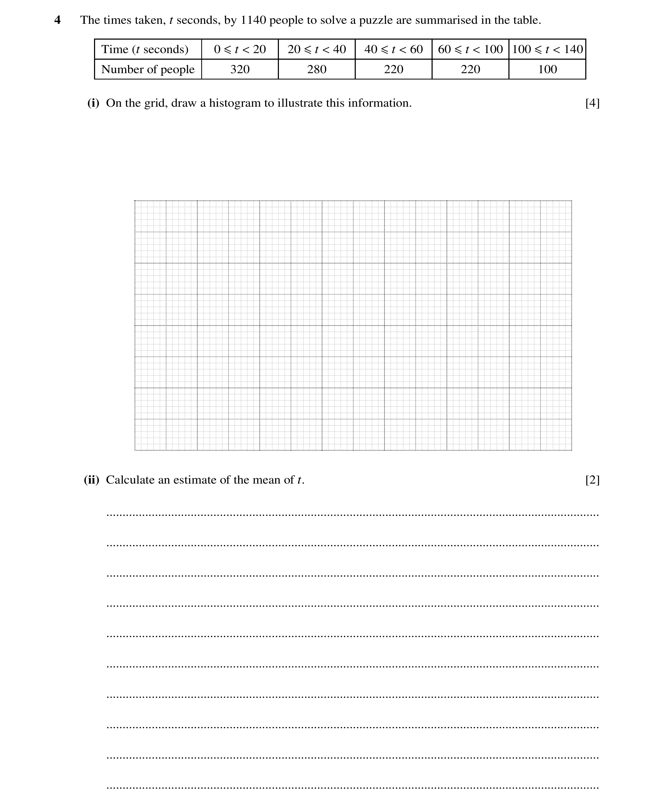 22 / 86
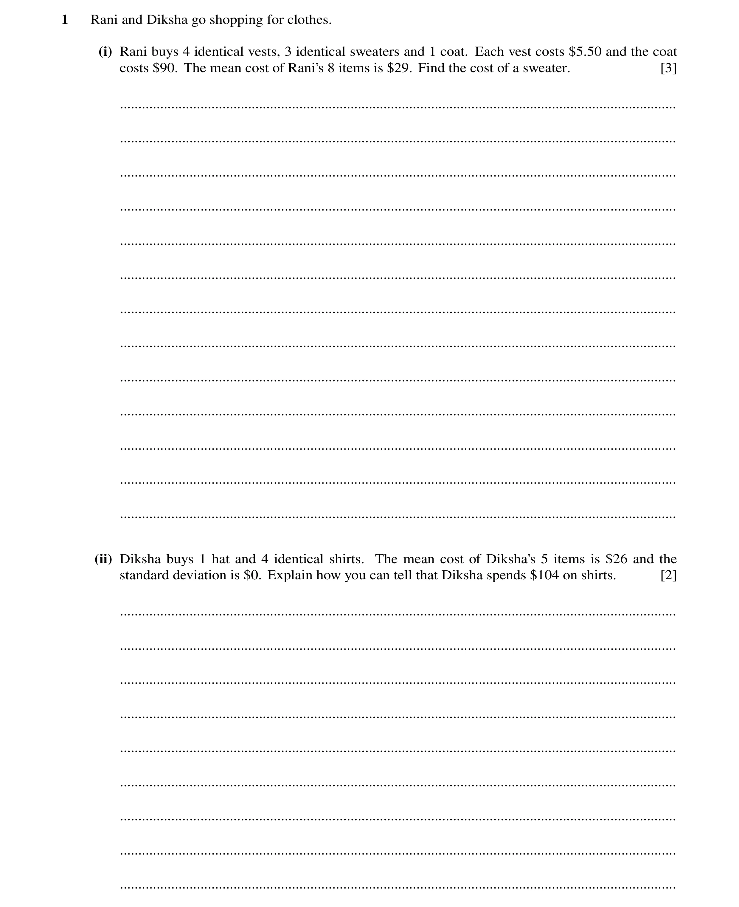 23 / 86
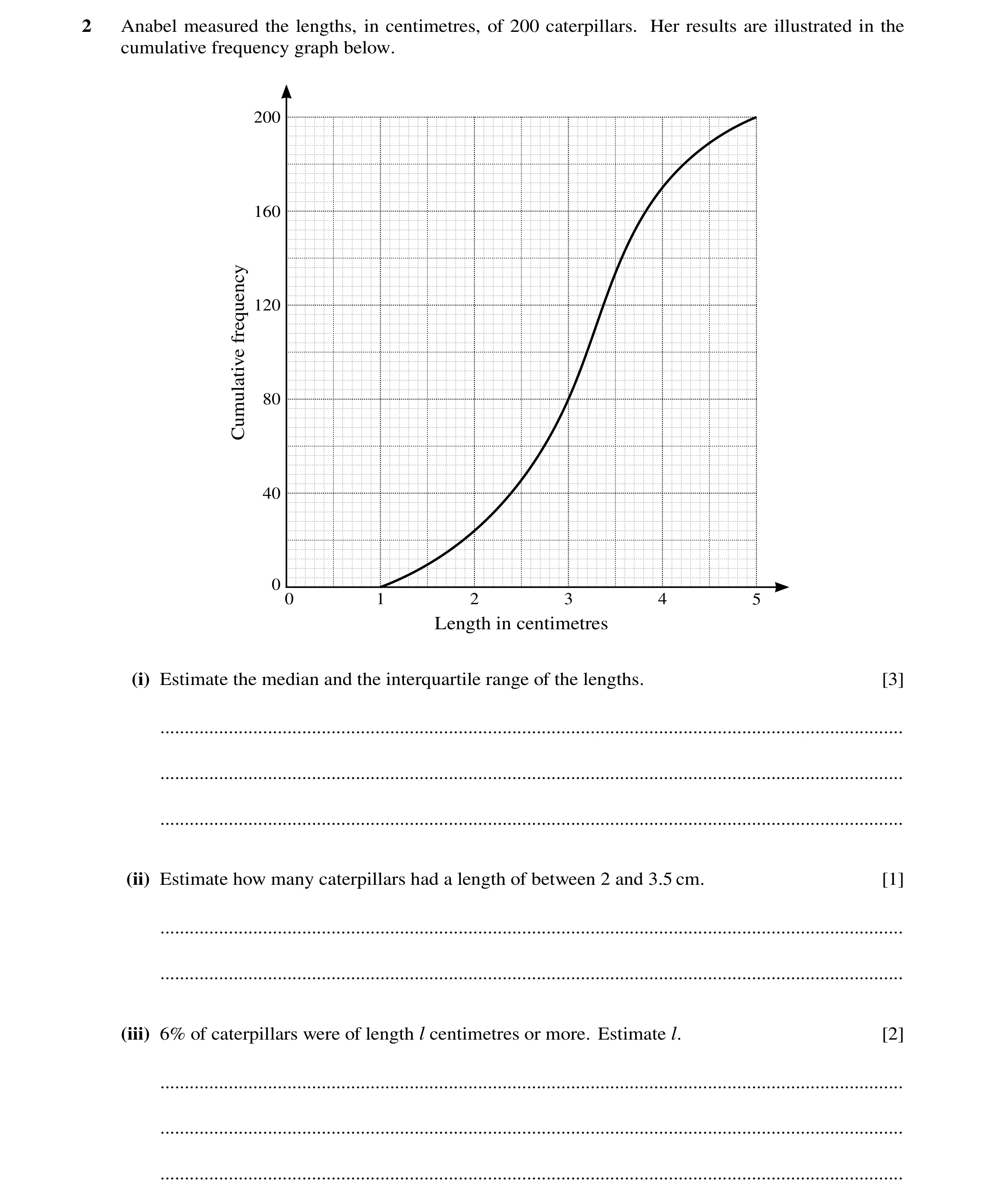 24 / 86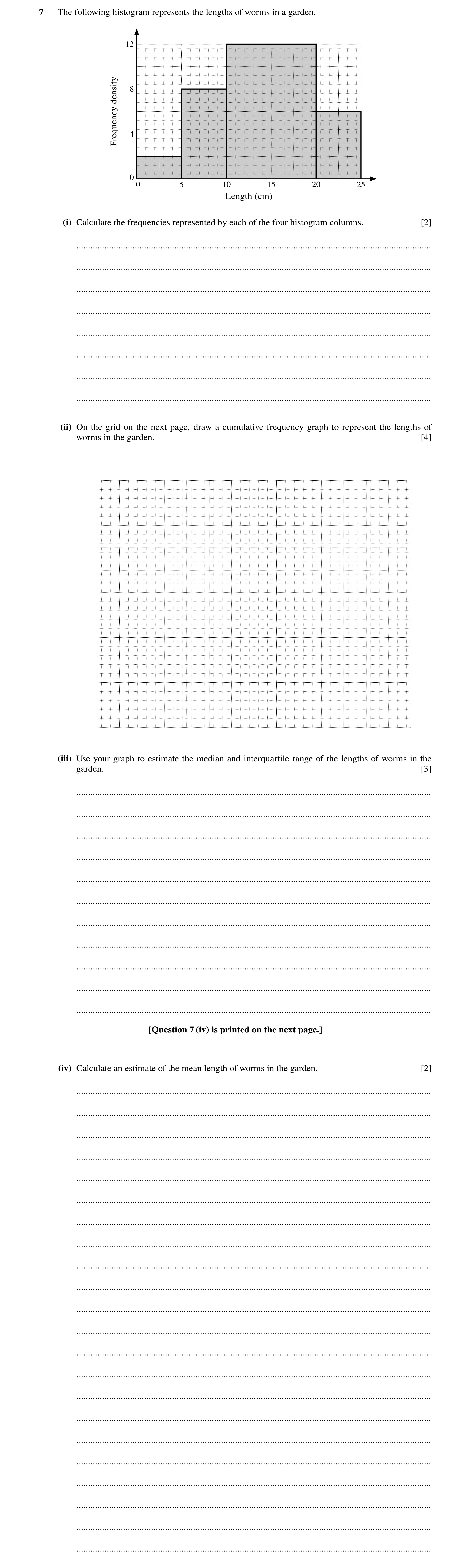
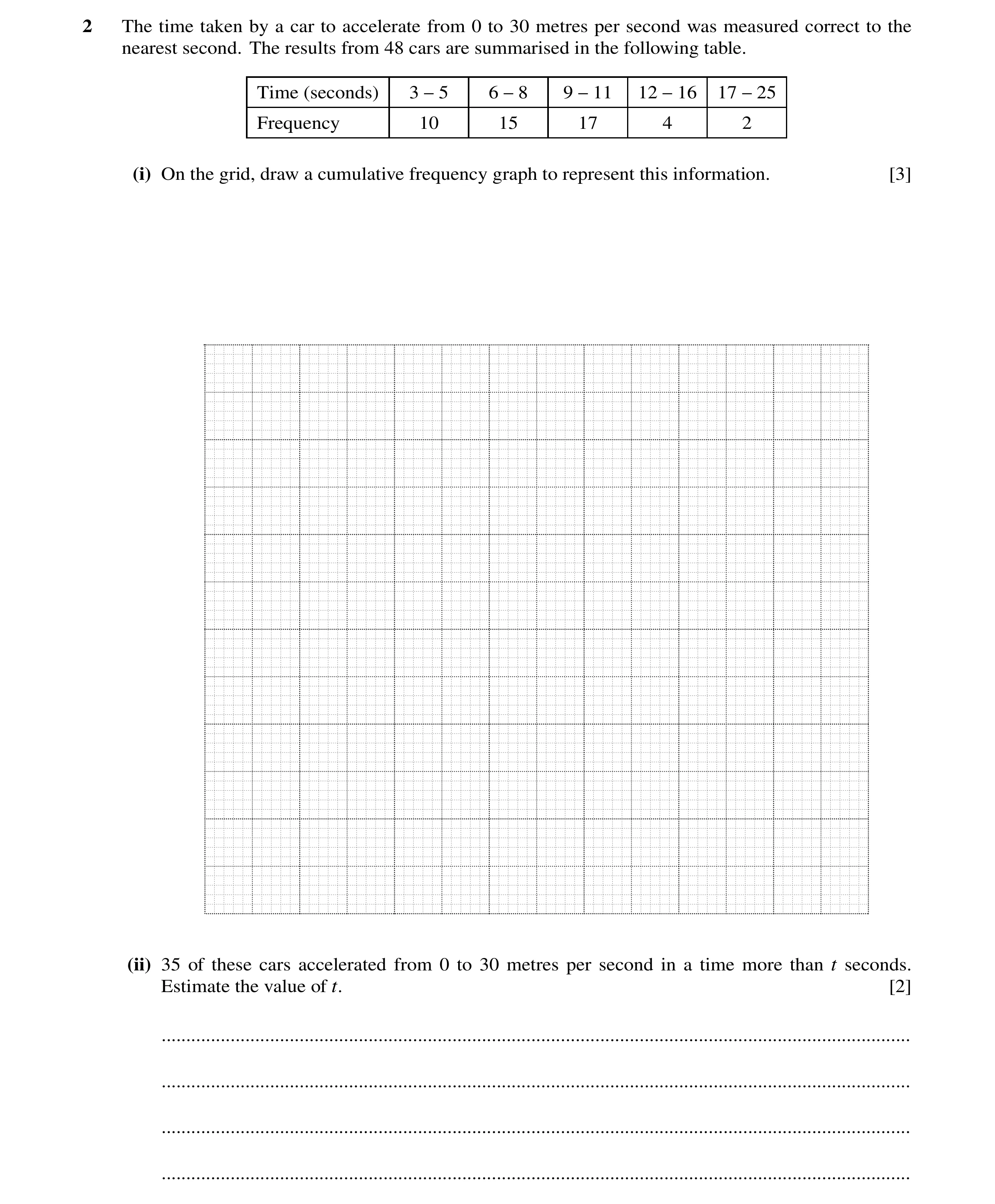 28 / 86
 29 / 86
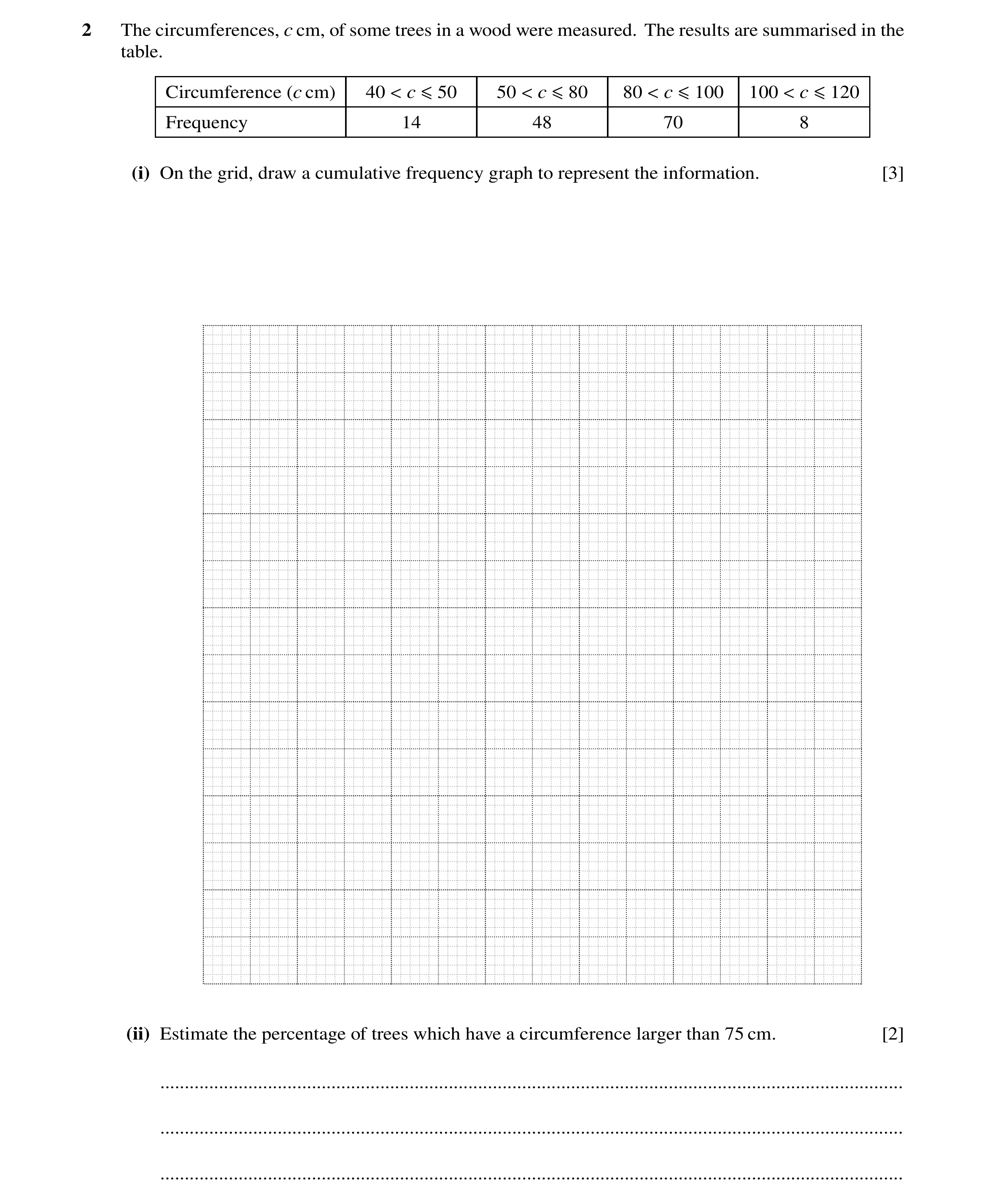 30 / 86
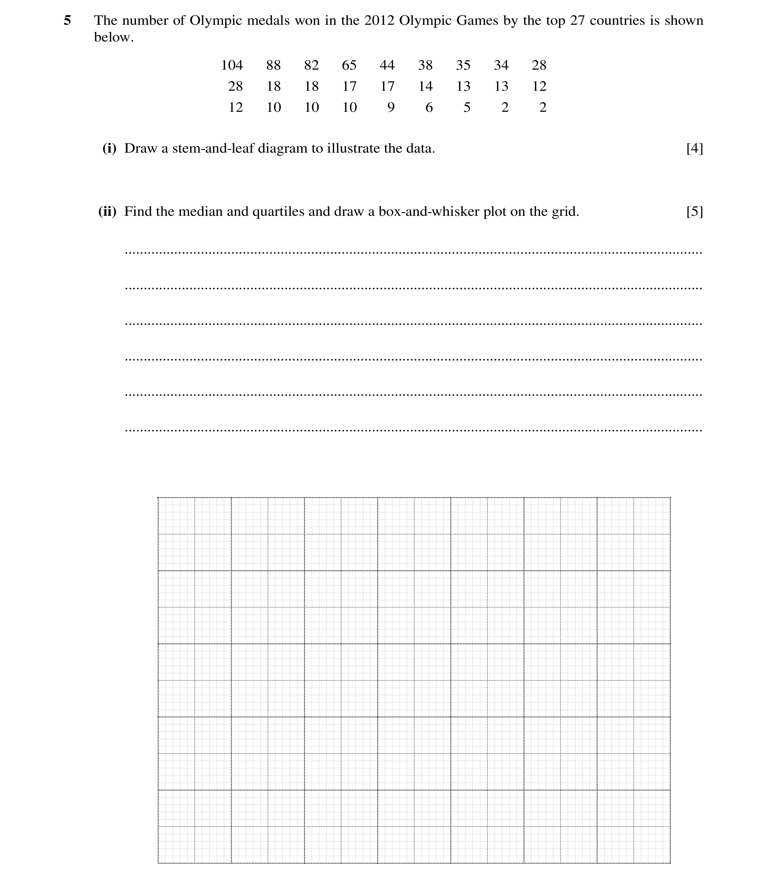 31 / 86
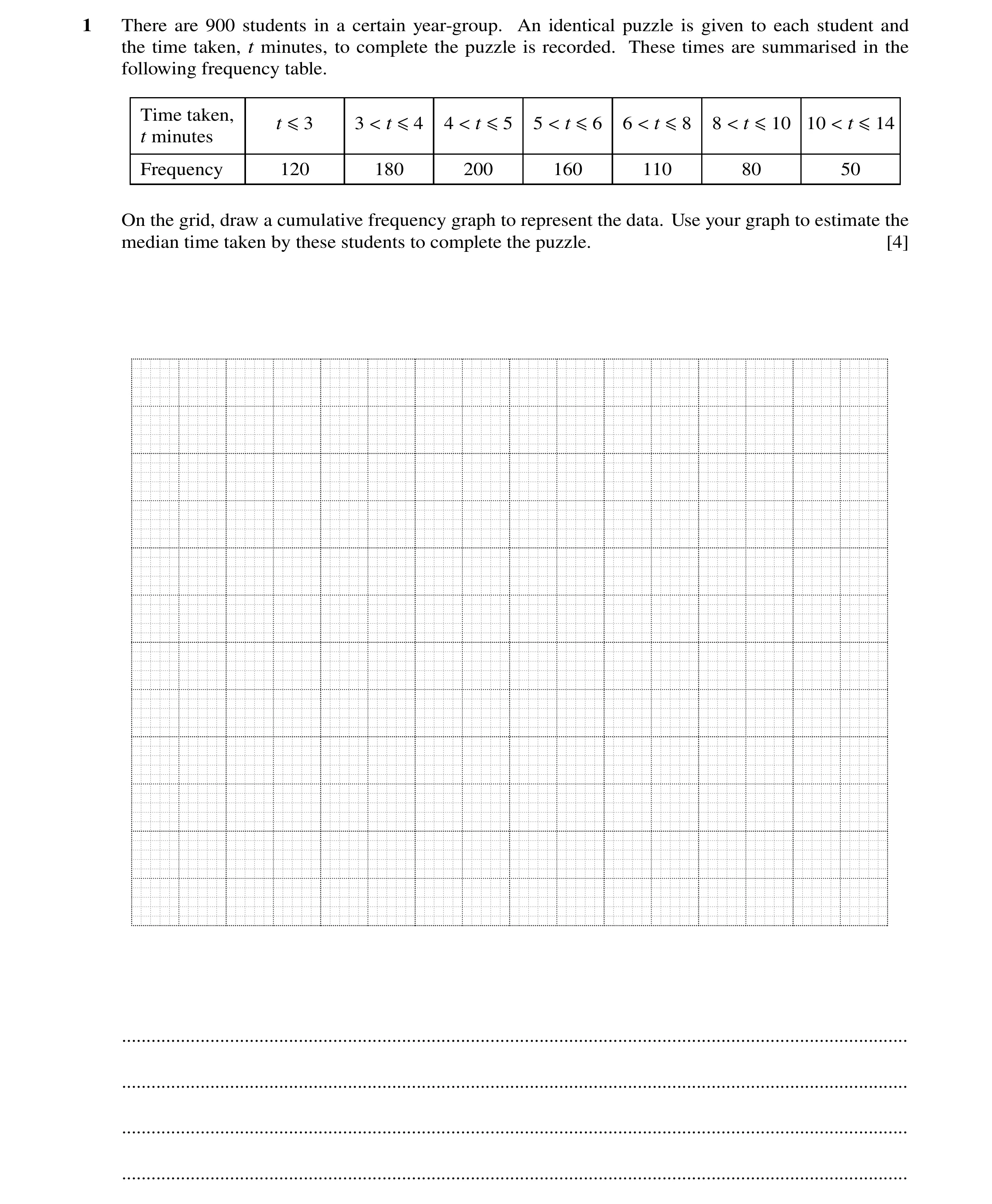 32 / 86
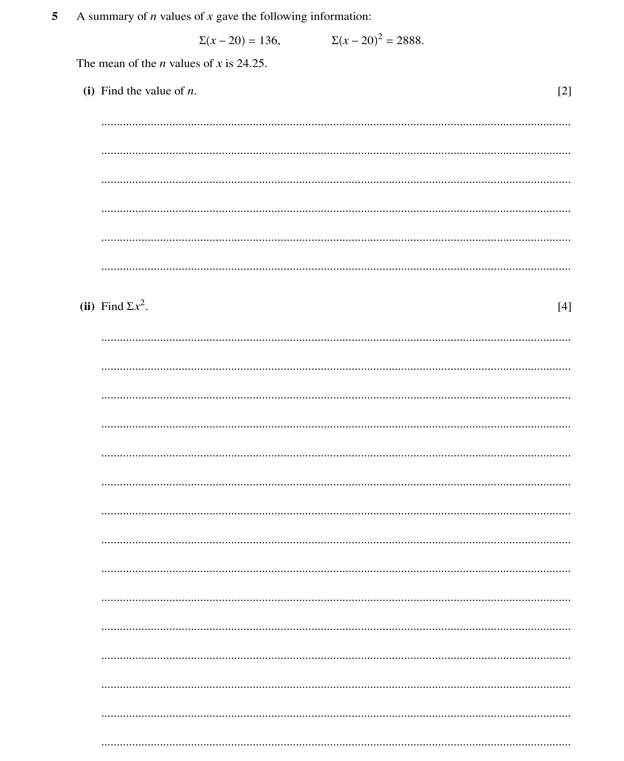 33 / 86
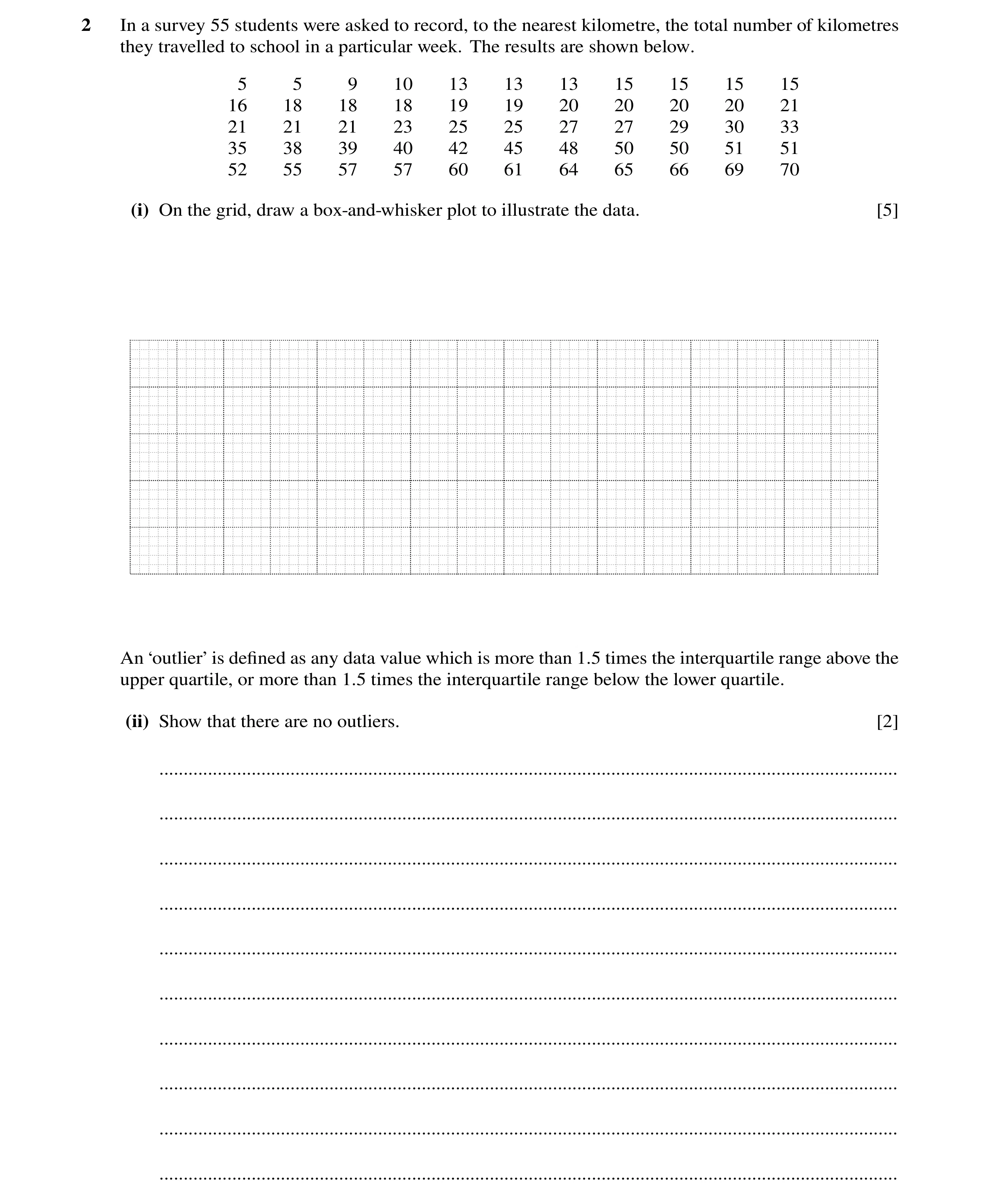 34 / 86
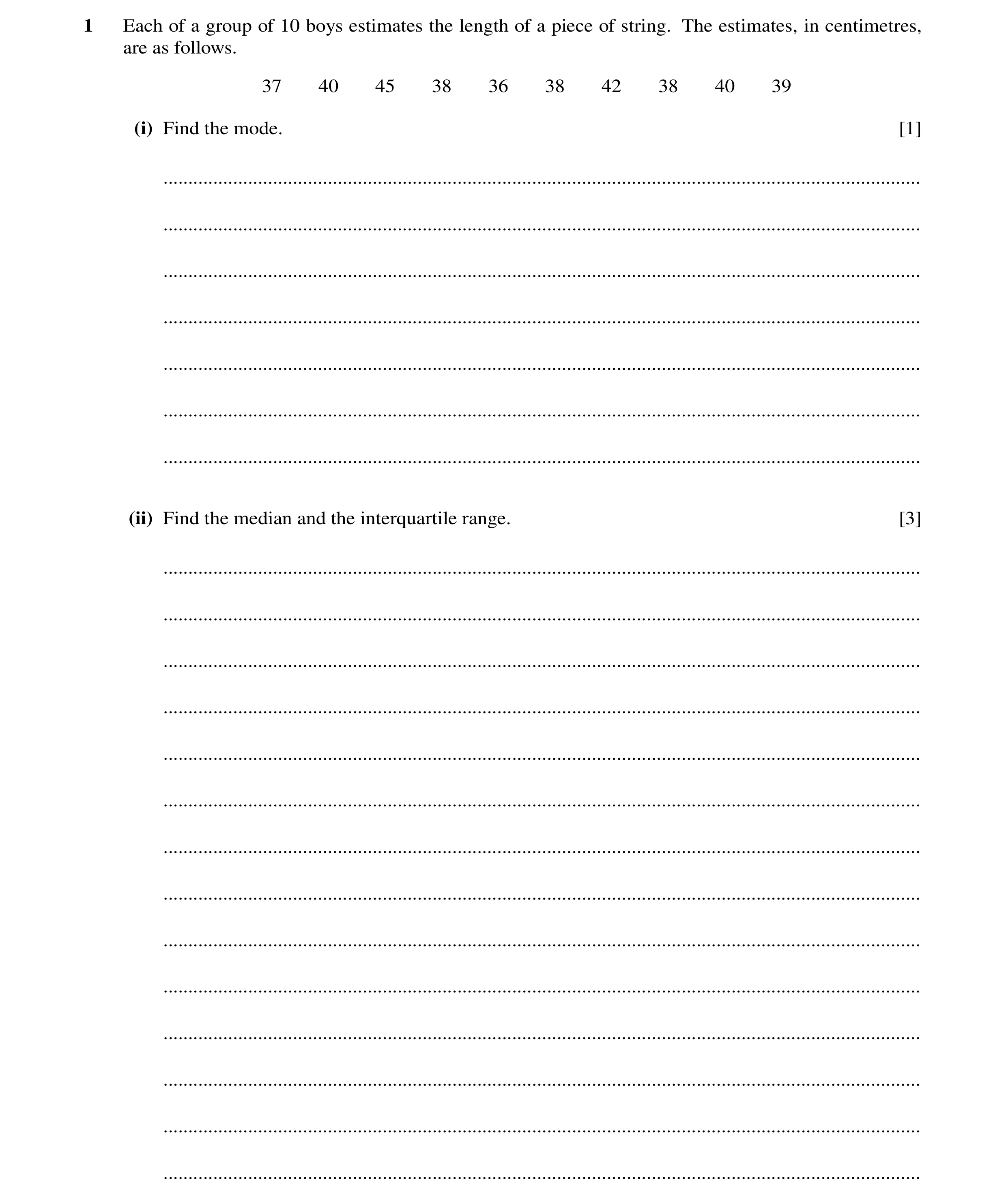 35 / 86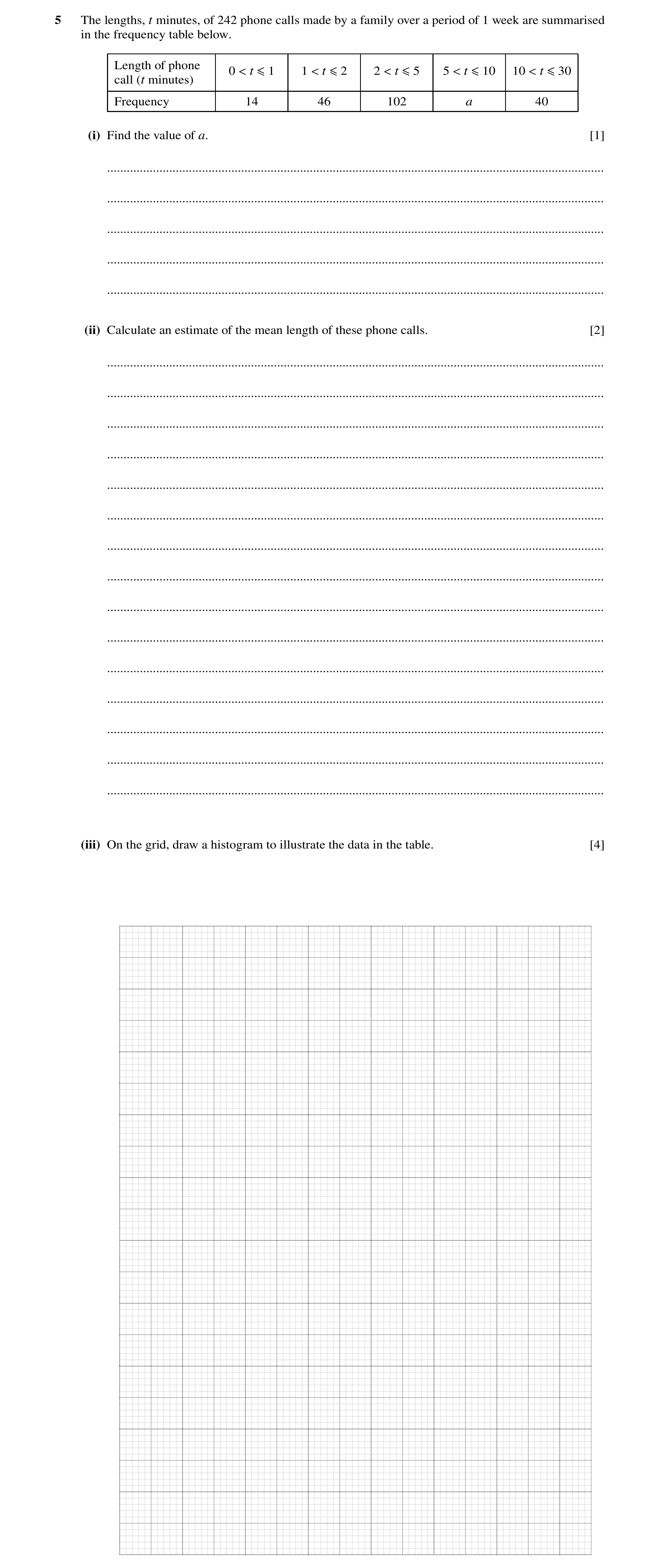
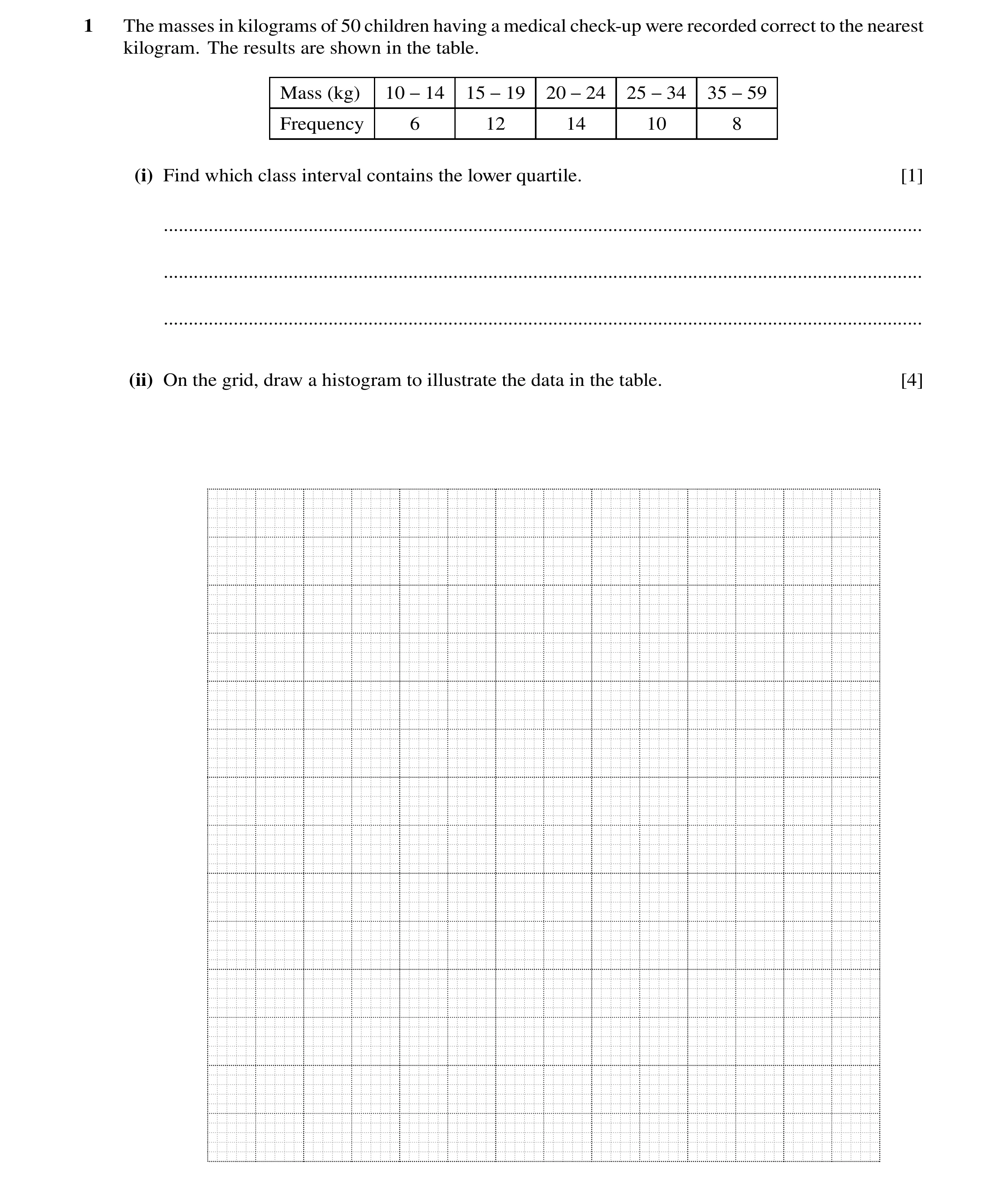 38 / 86
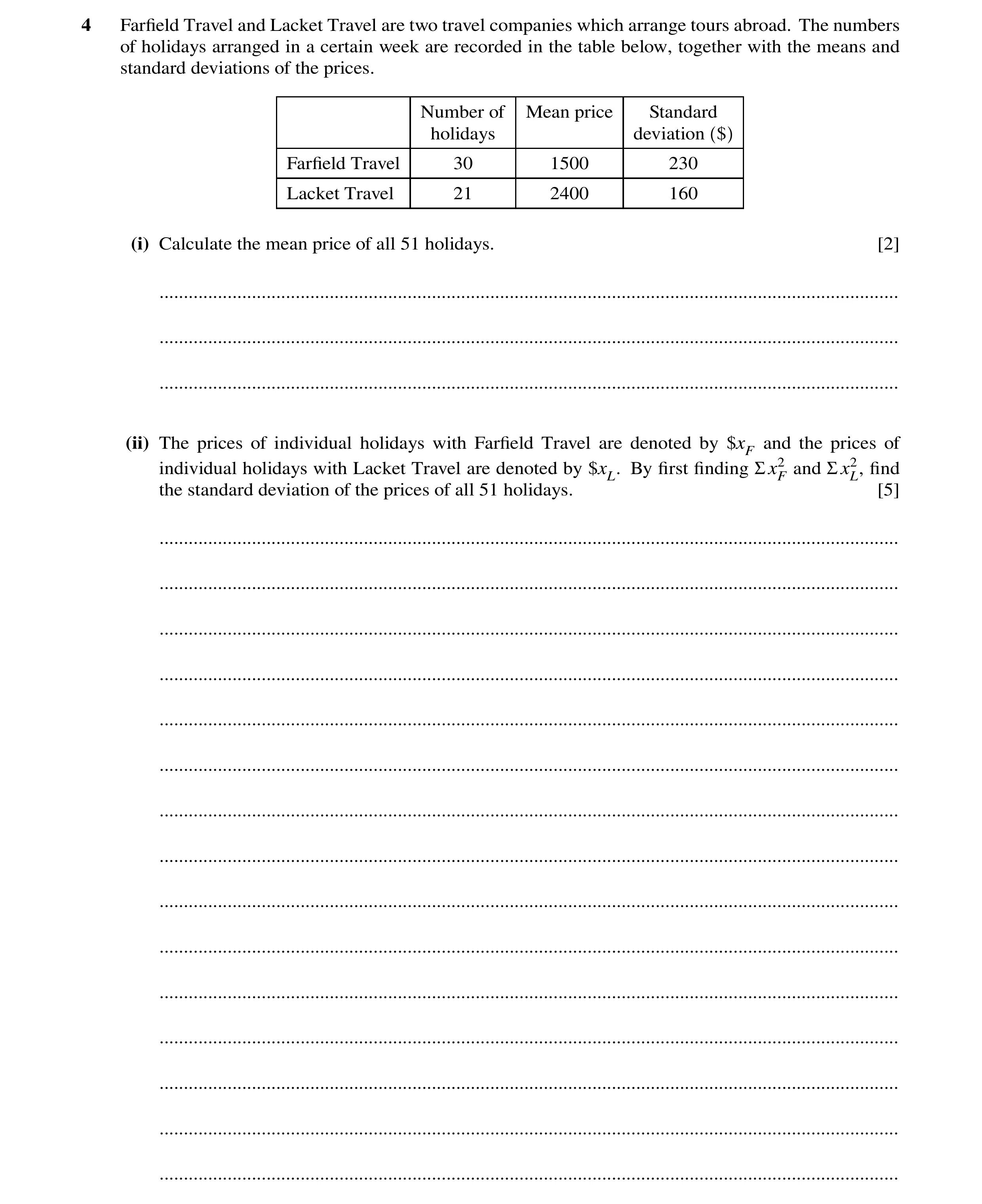 39 / 86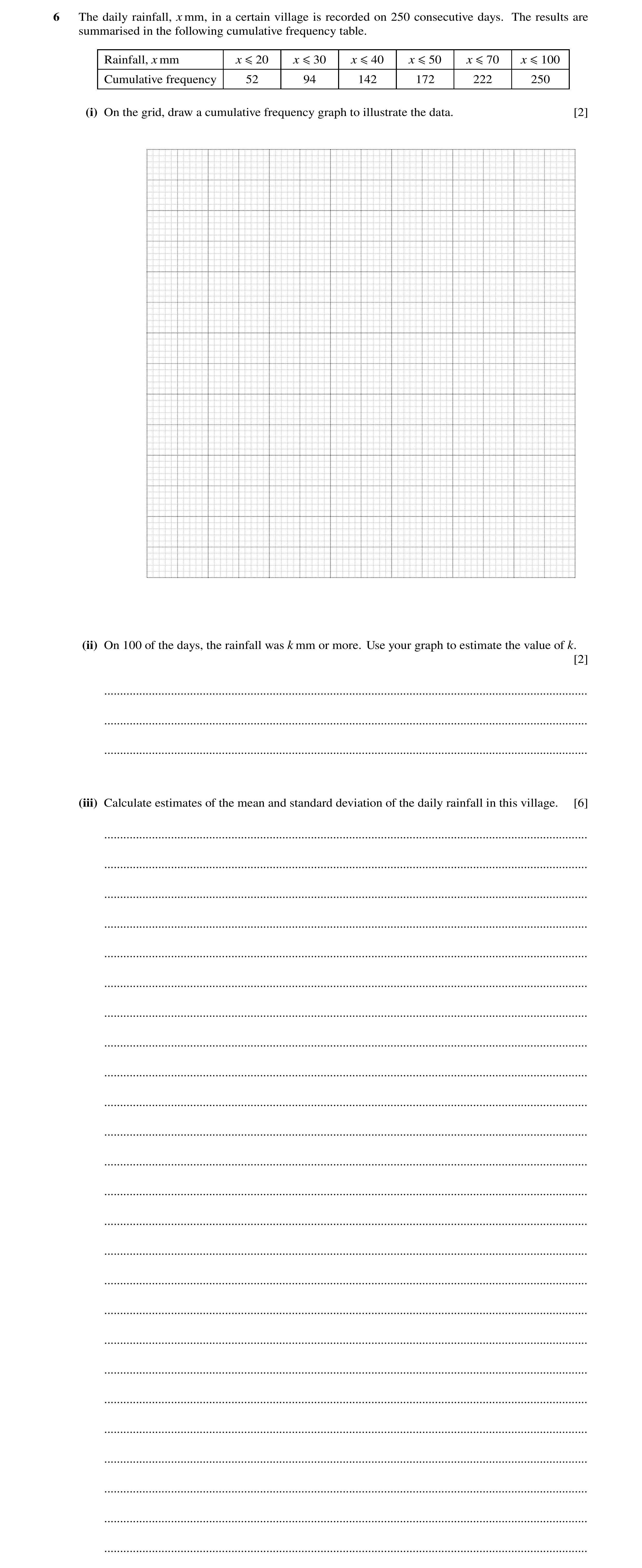
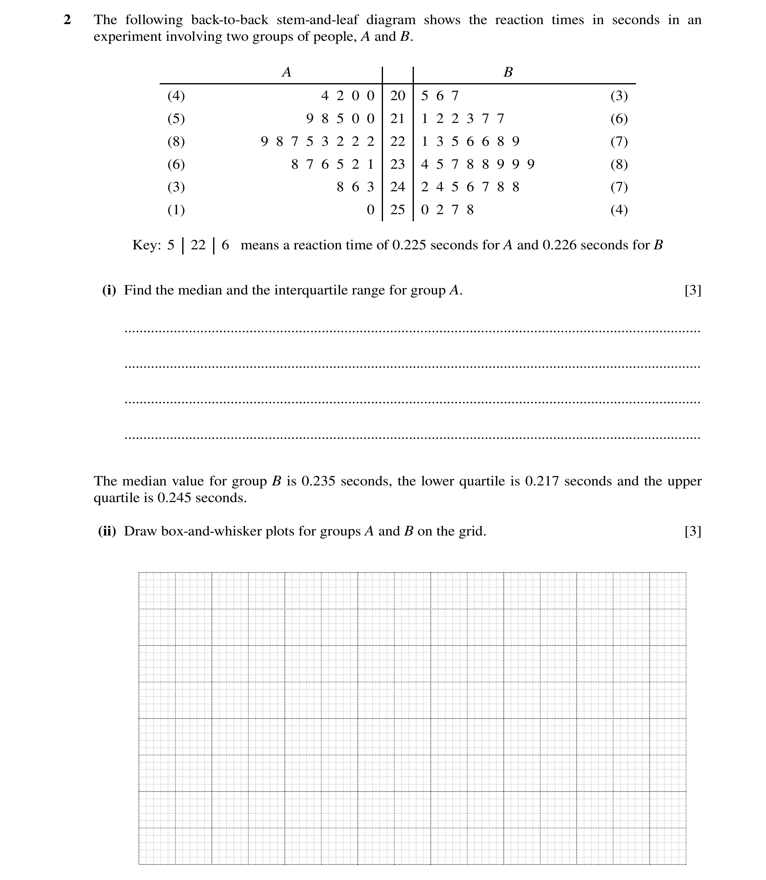 42 / 86
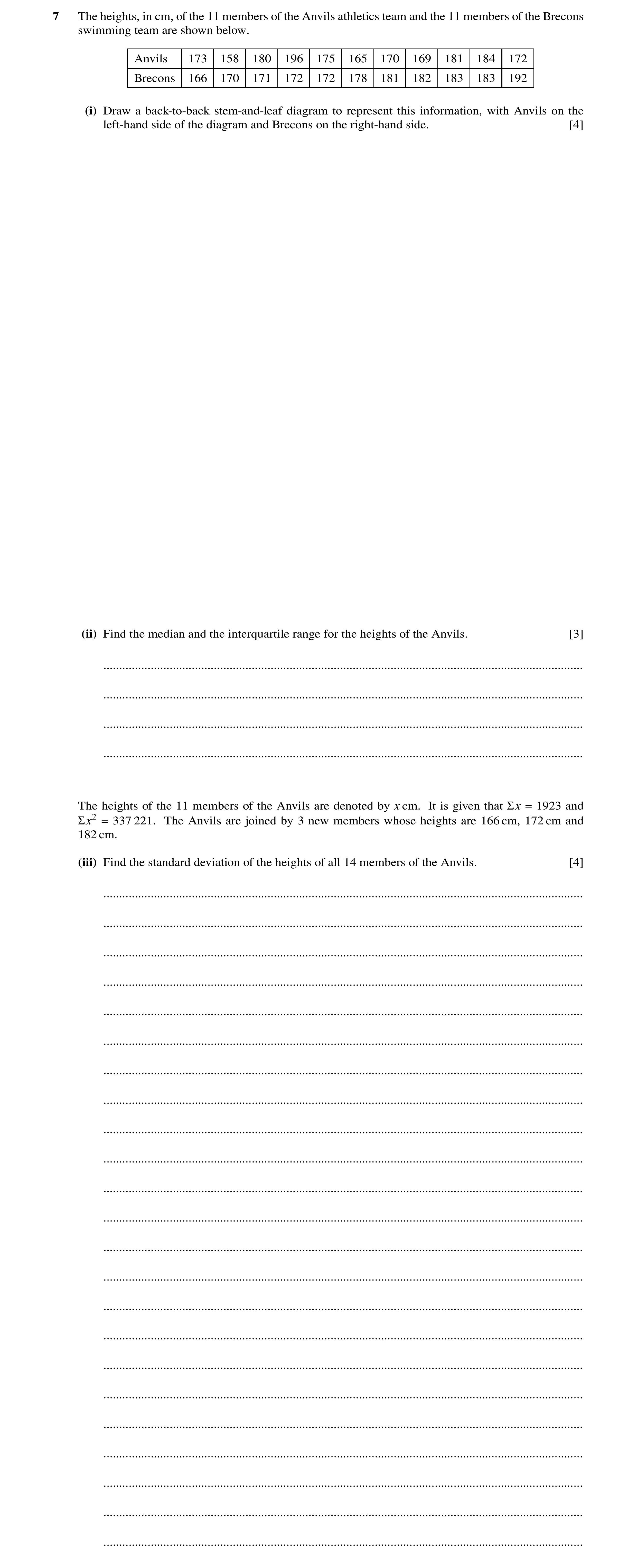
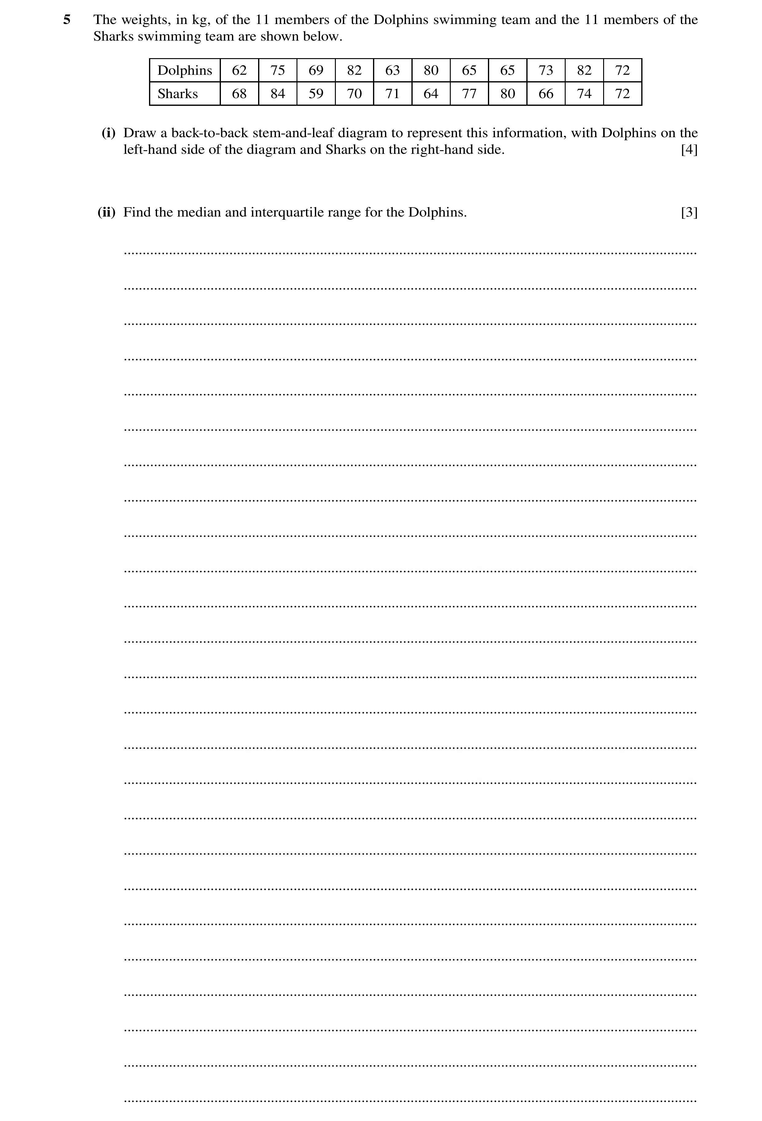
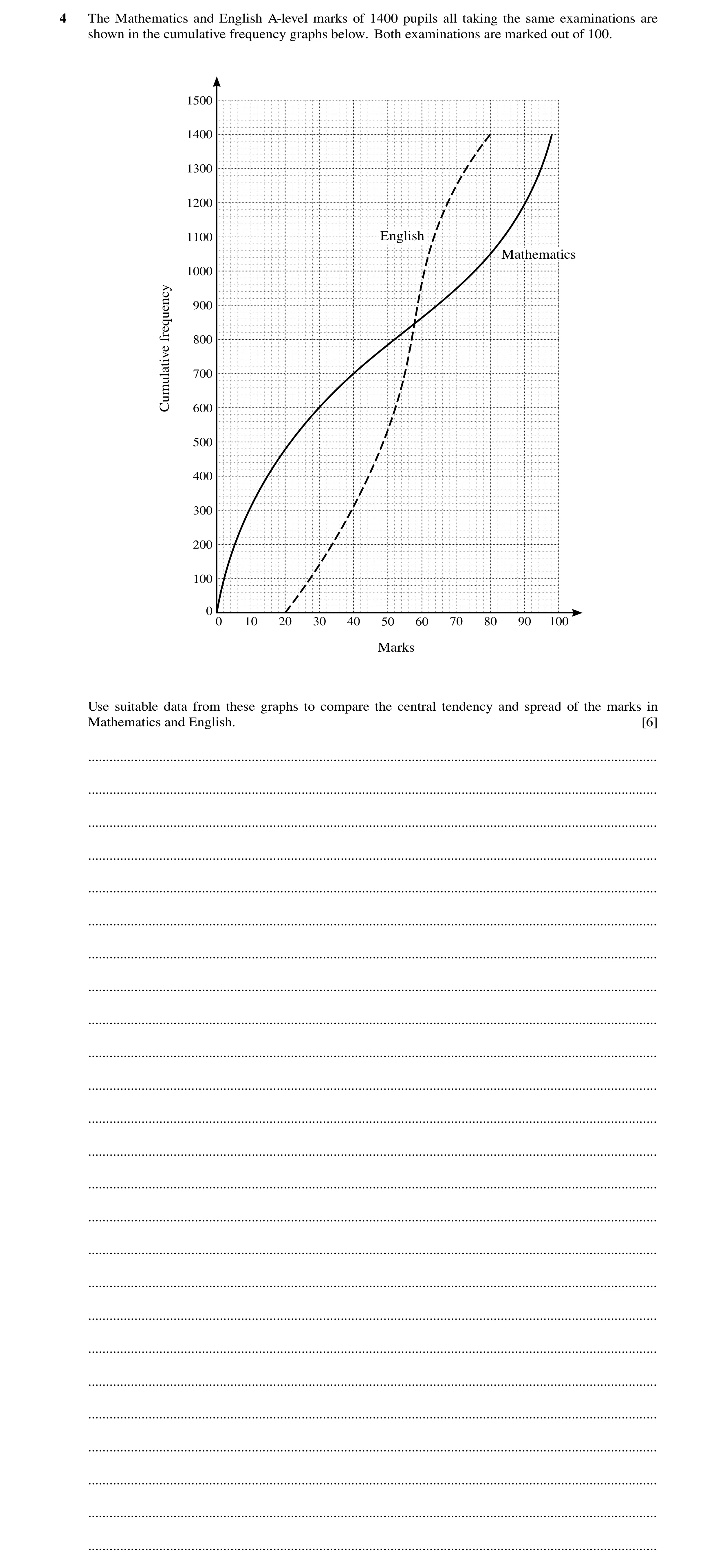
![Question 77: (i) Give one advantage and one disadvantage of using a box-and-whisker plot to represent a set of data. [2] ...............................…](https://img.pastlit.com/crops/6dda13f7-c186-4ef1-a0a3-2d83c7132d90/q6.webp)
![Question 78: The mean and standard deviation of 20 values of x are 60 and 4 respectively. (i) Find the values of Σx and Σx2. [3] .......................…](https://img.pastlit.com/crops/a4b29434-06f6-4be3-a1ac-8ec32d362b97/q3.webp)
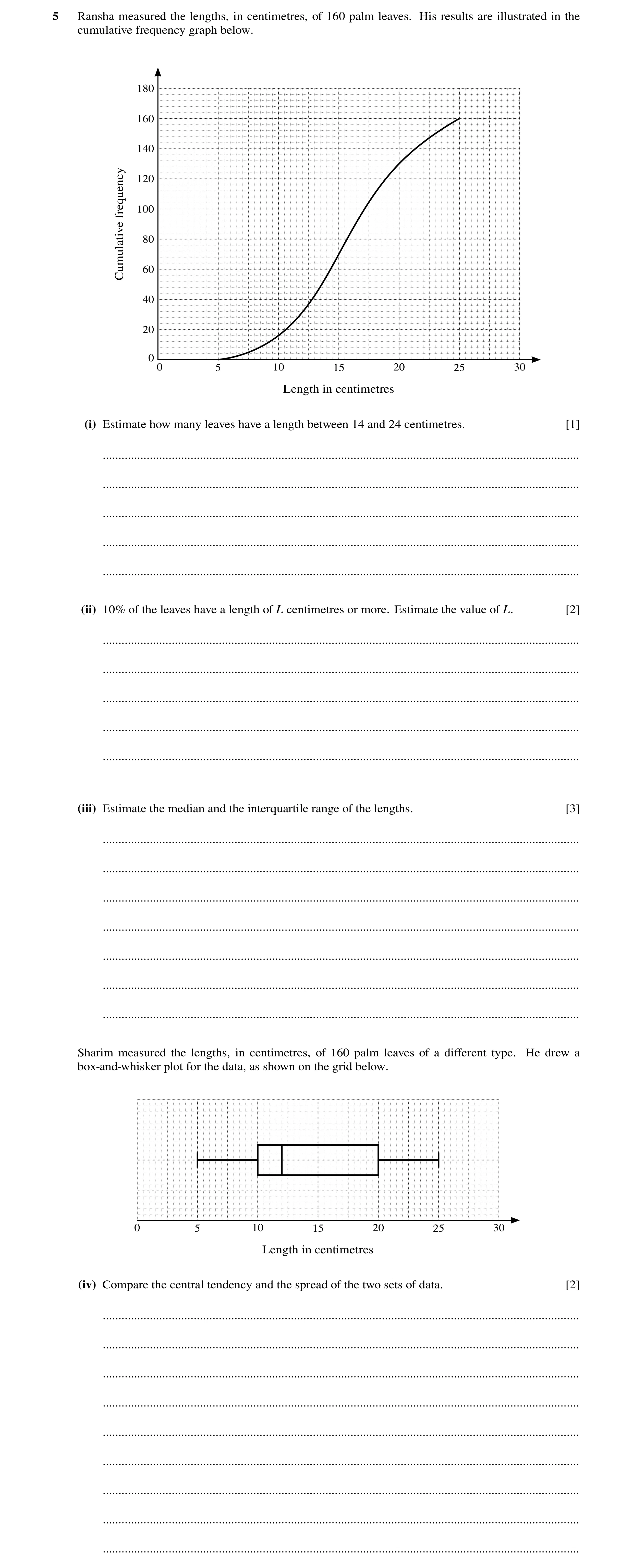
 55 / 86
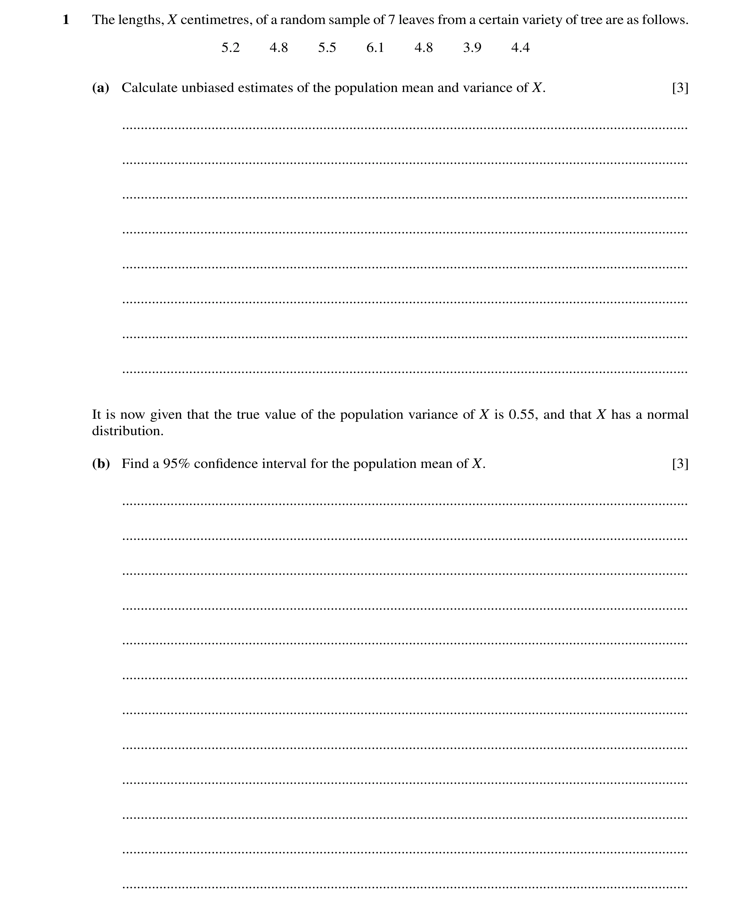 60 / 86
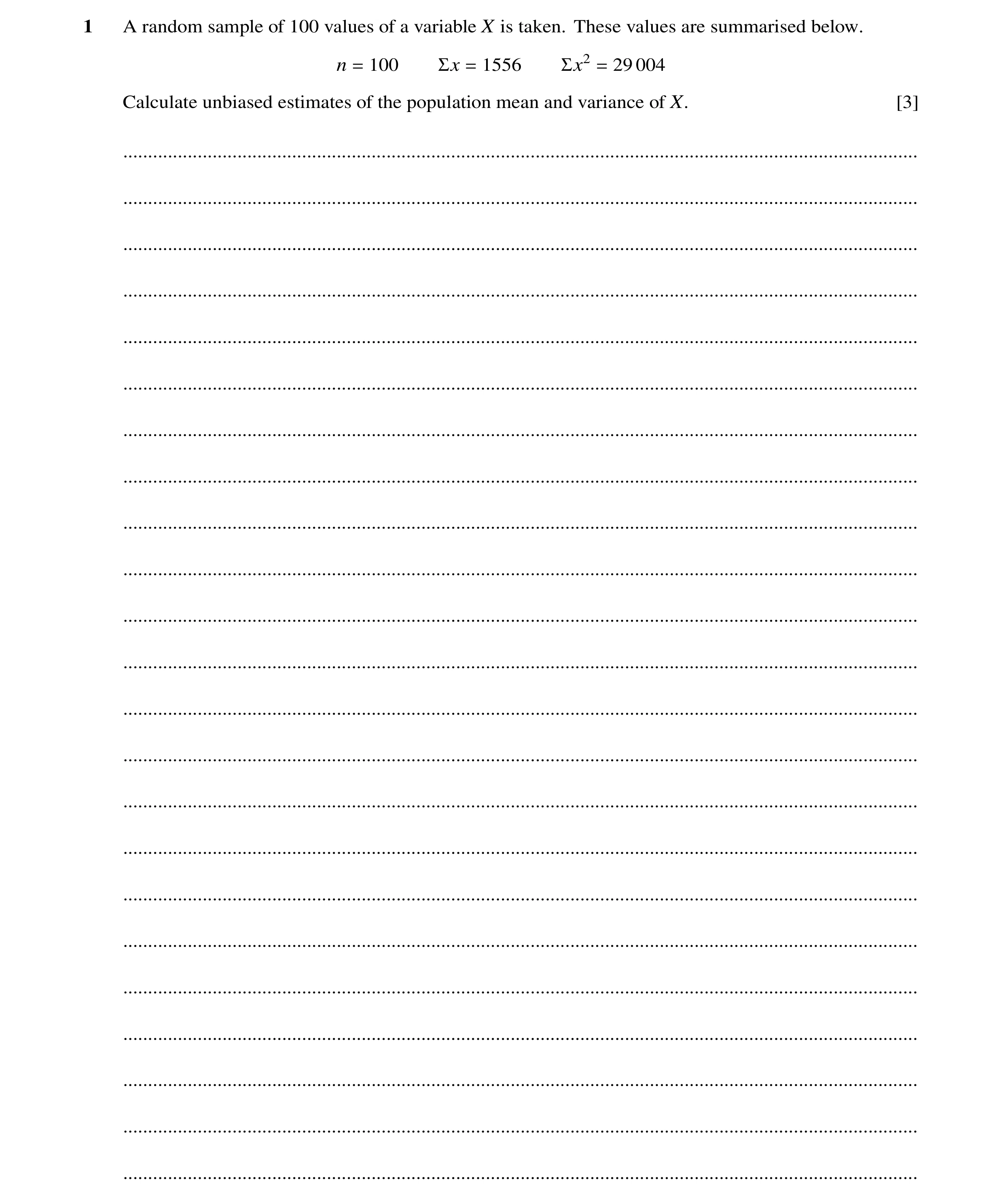 61 / 86
 68 / 86
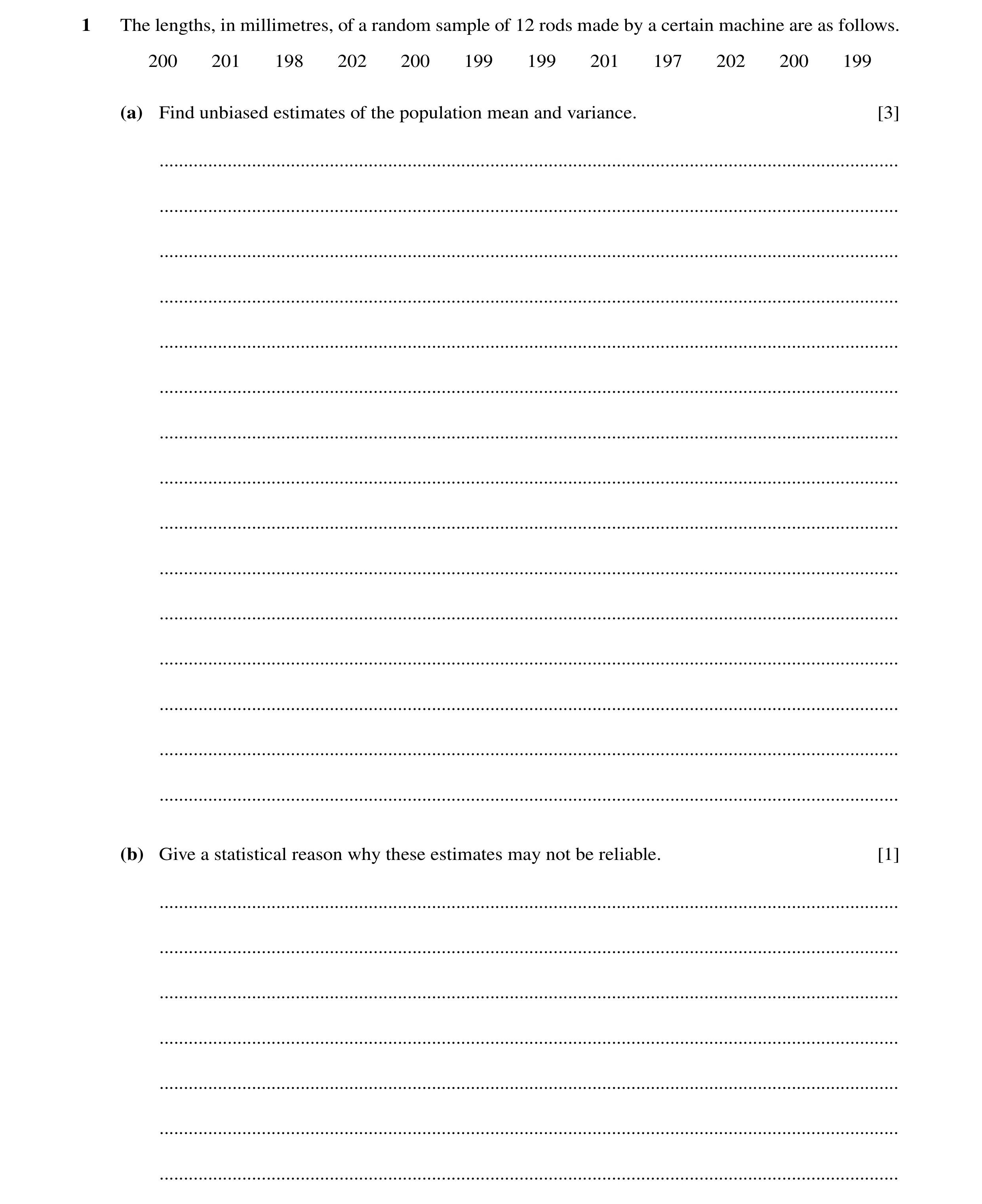 69 / 86
 70 / 86
 71 / 86
 72 / 86
 75 / 86
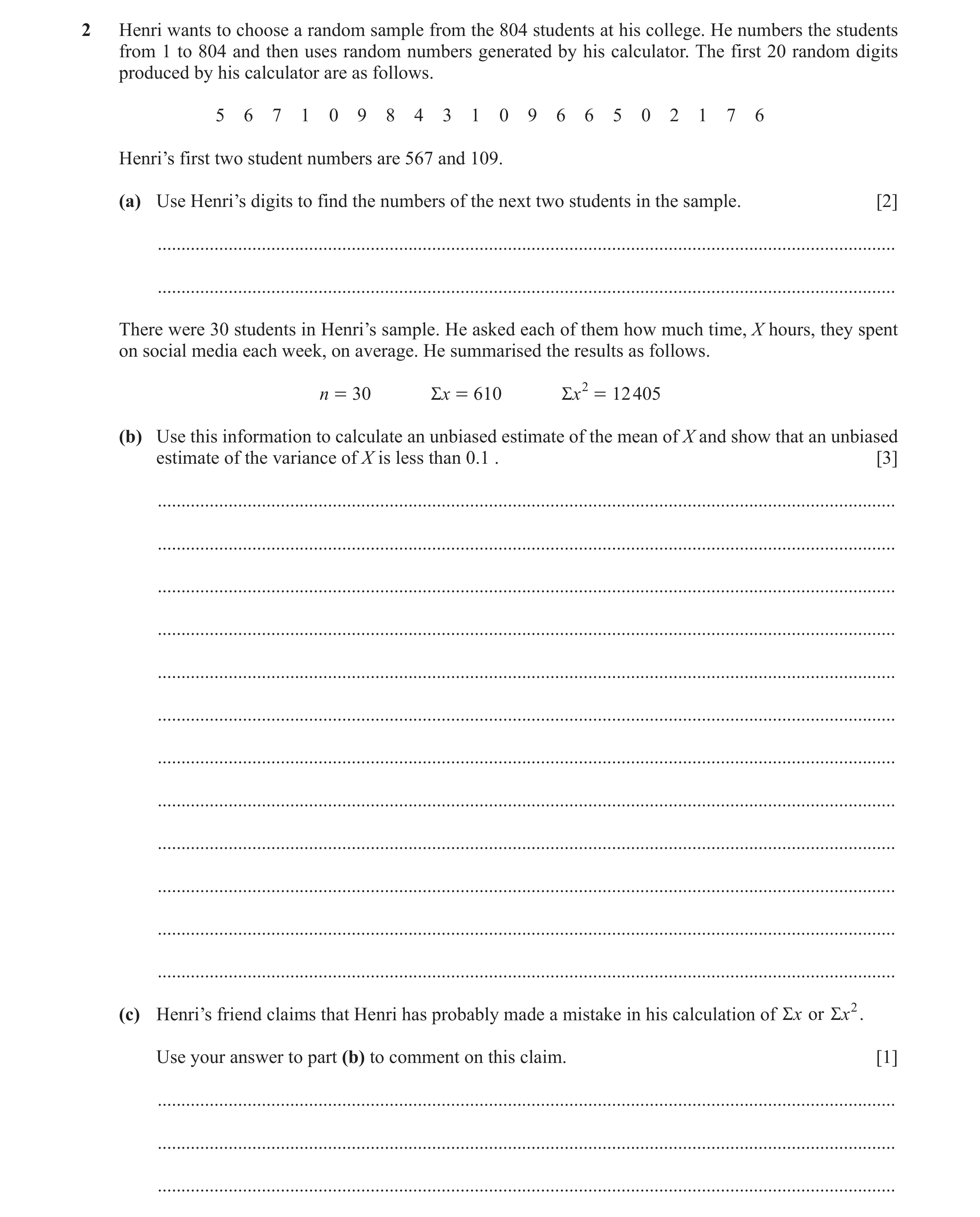 76 / 86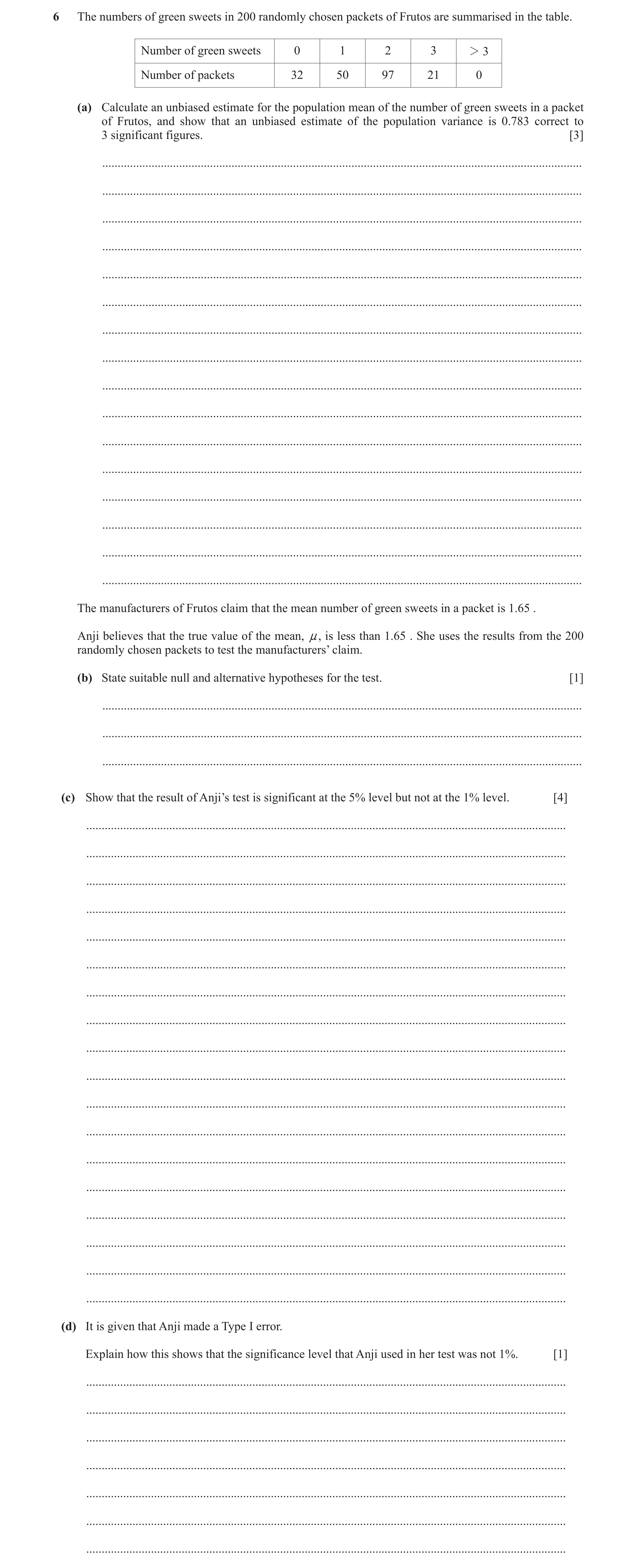
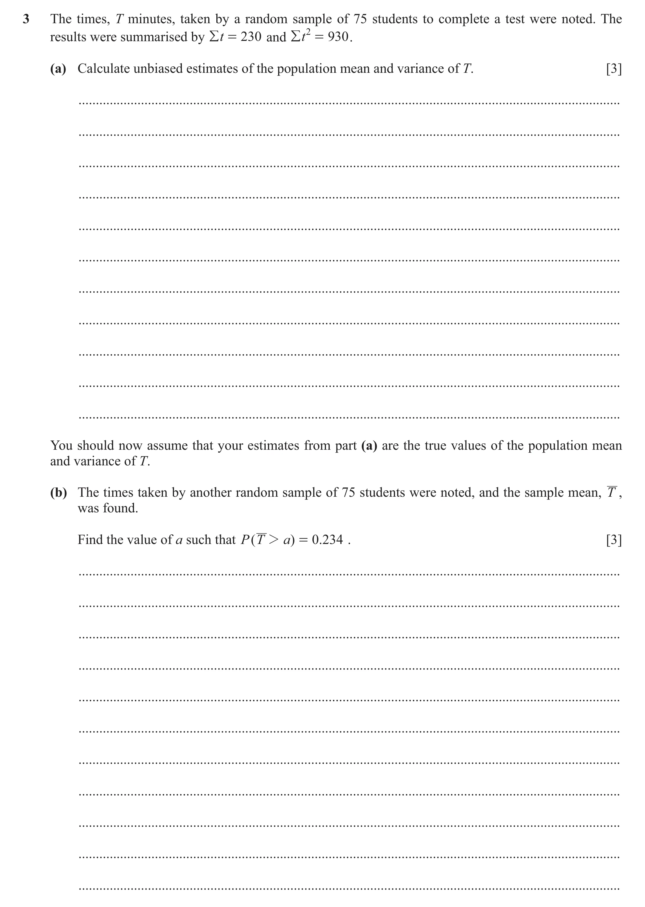 79 / 86
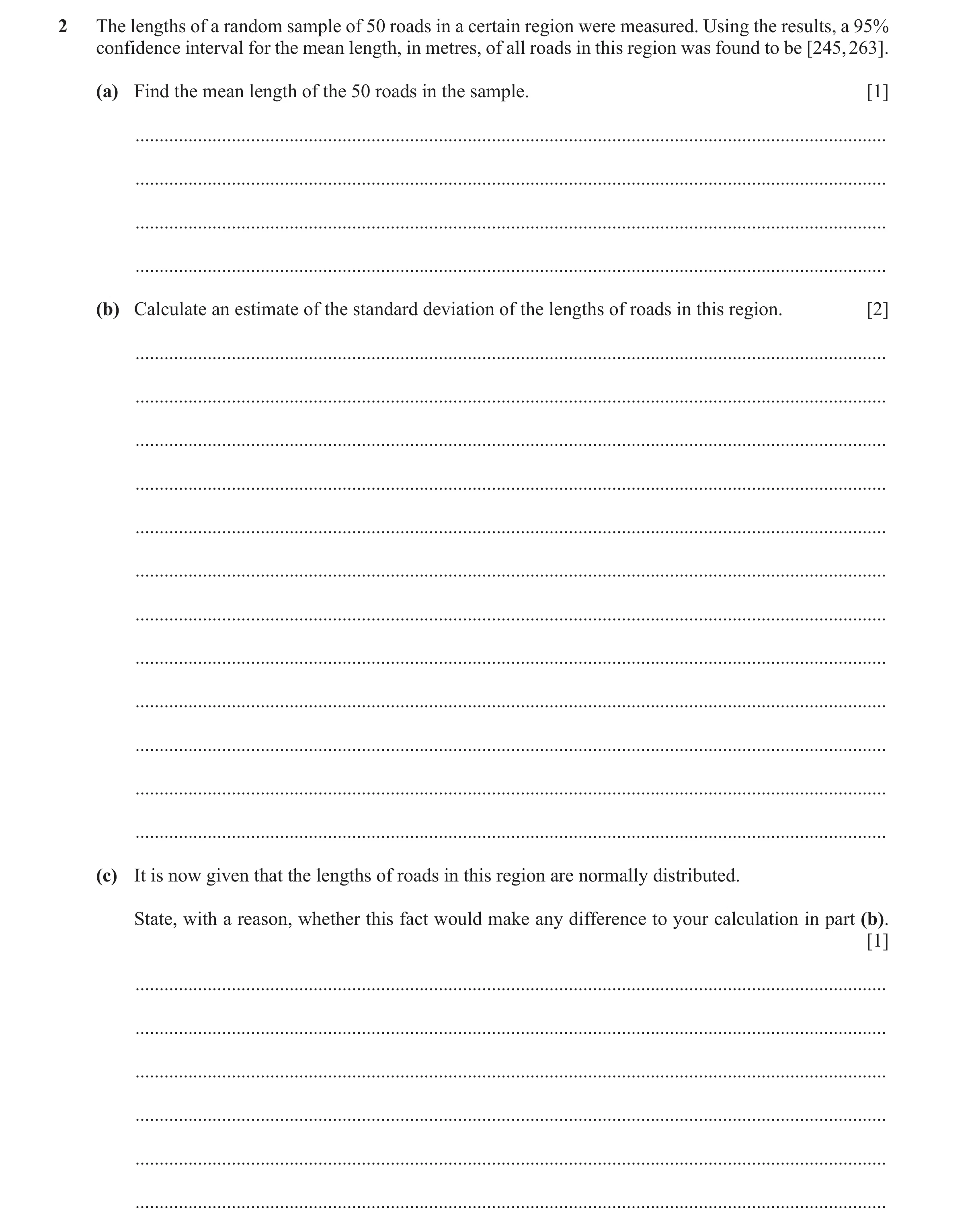 80 / 86
 83 / 86
 86 / 86
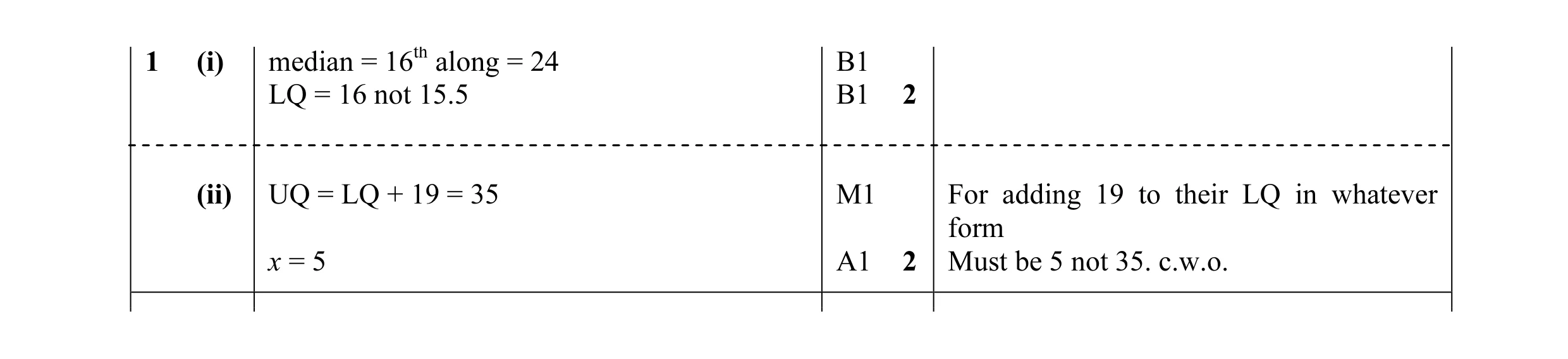 4
4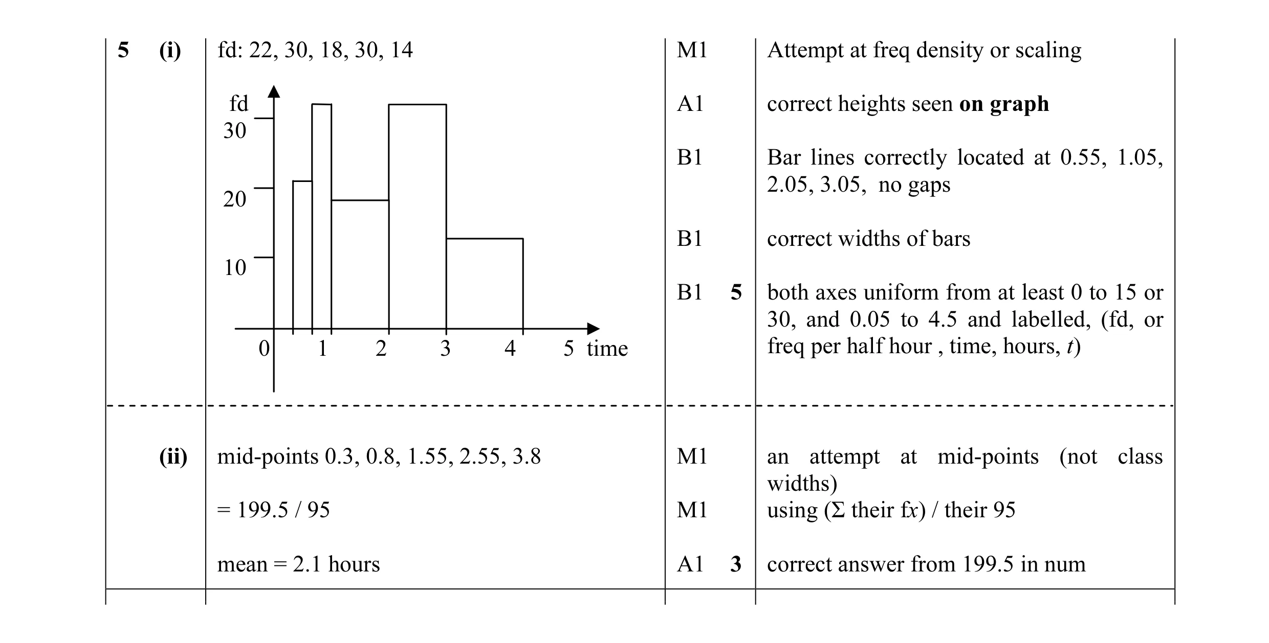 8
8 3
3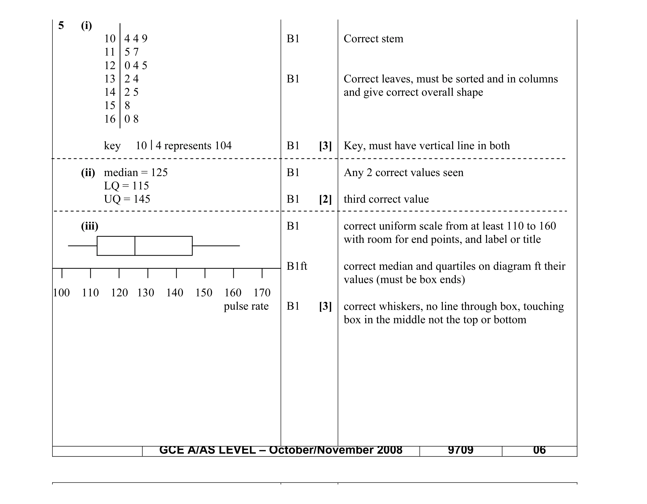 8
8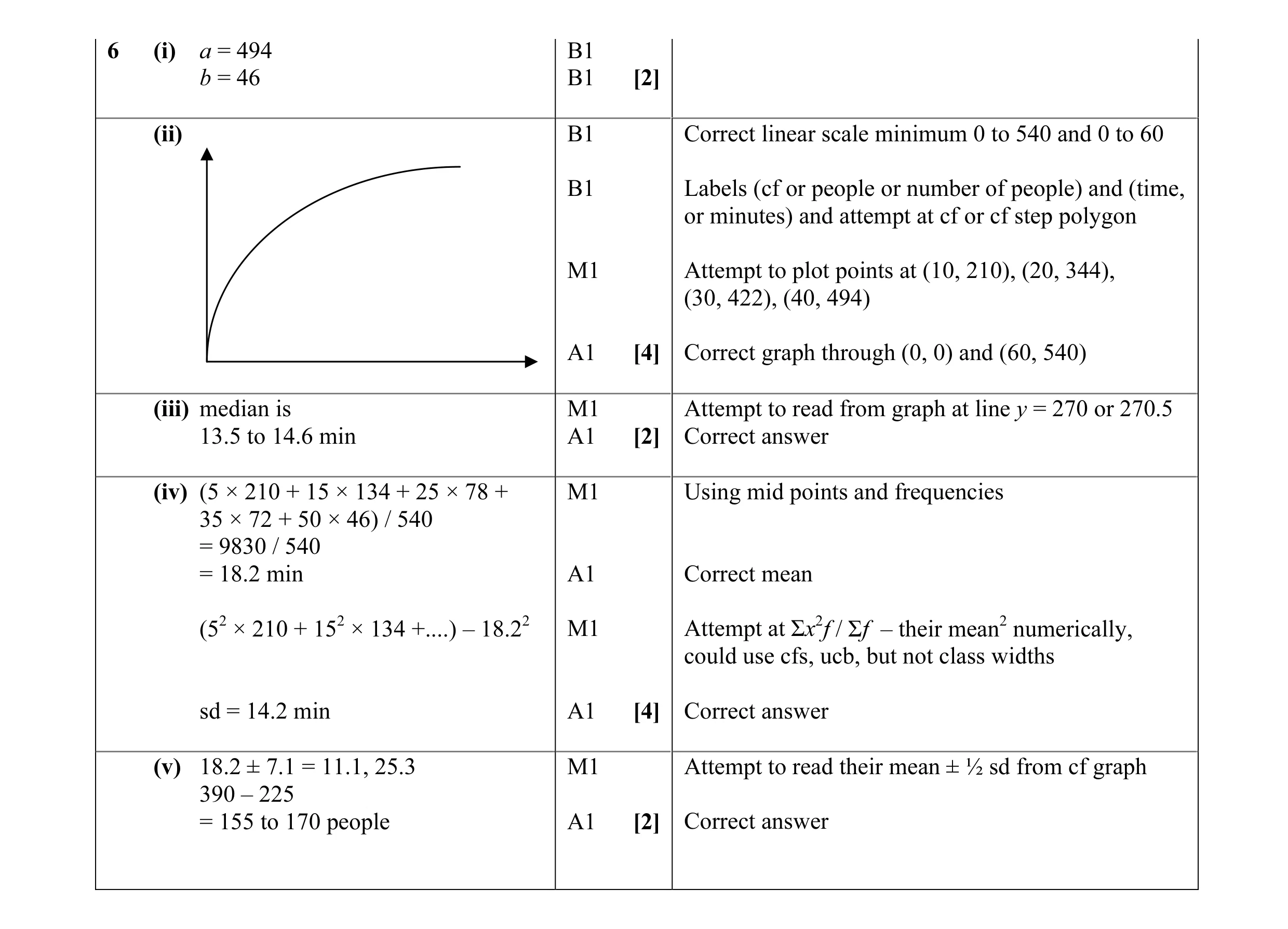 14
14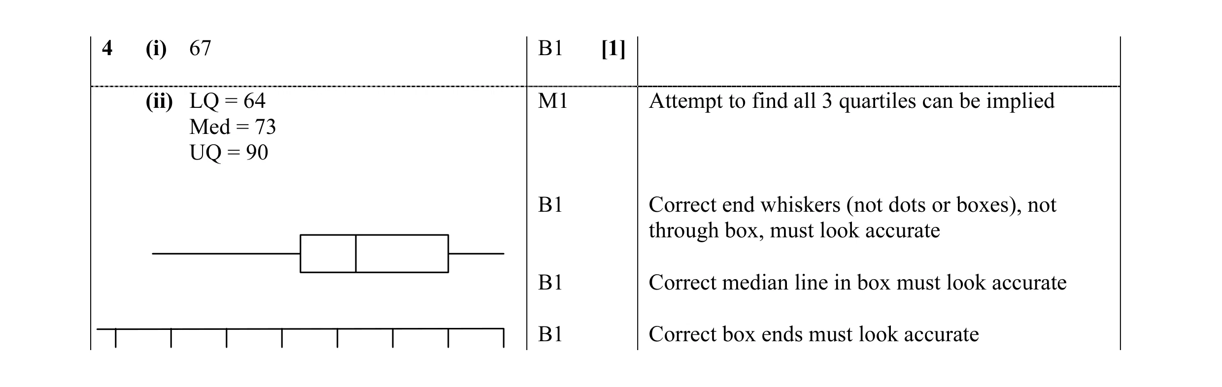 7
7 4
4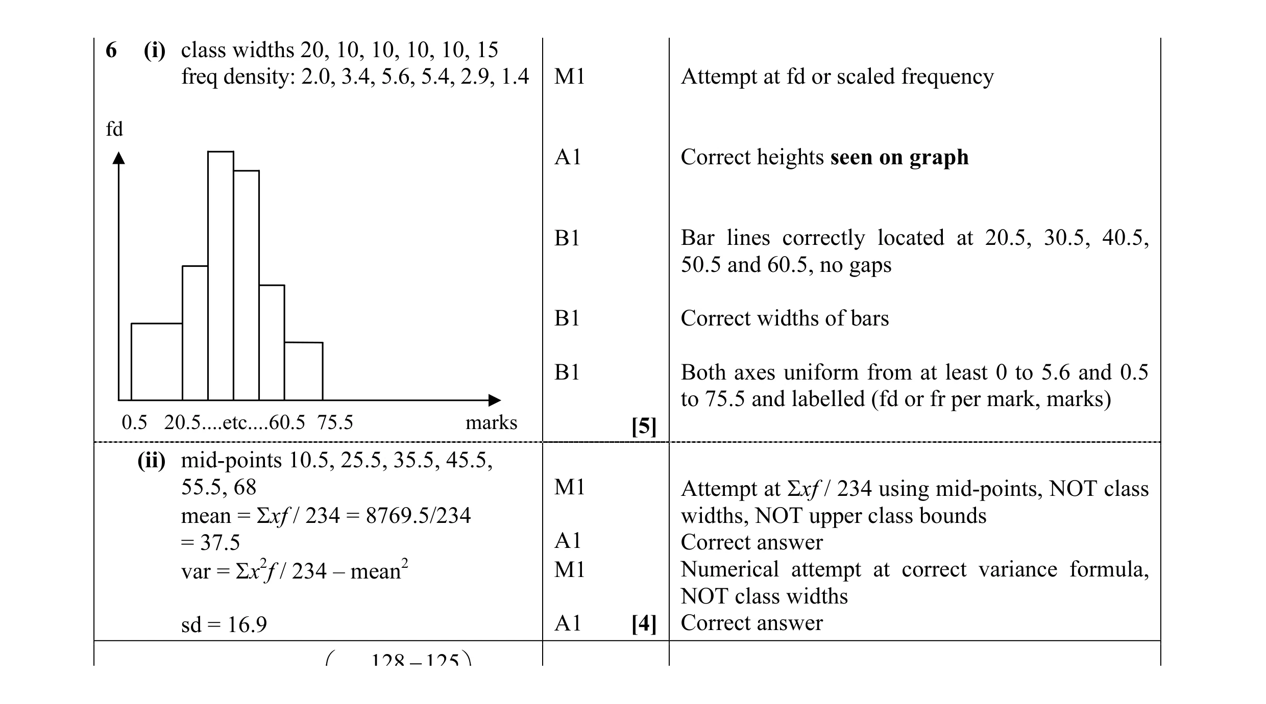 9
9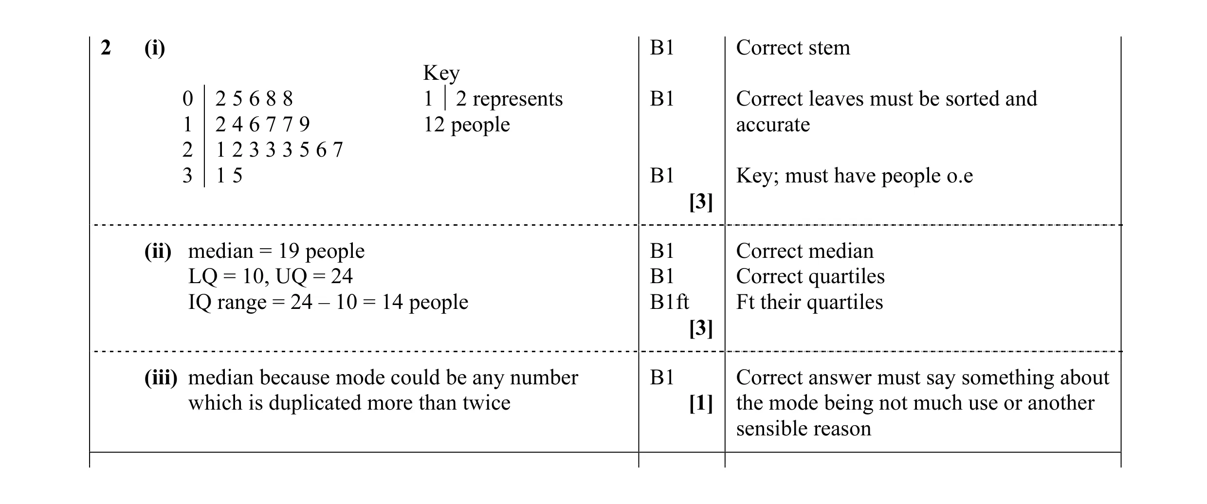 7
7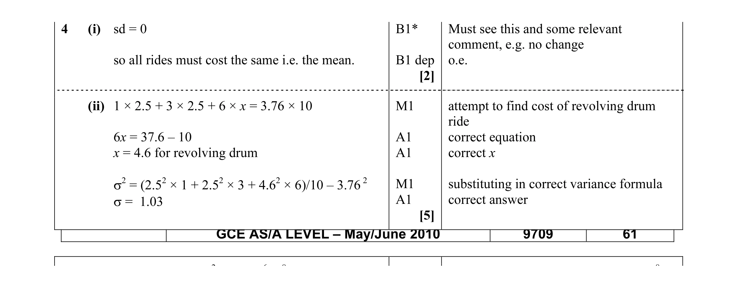 7
7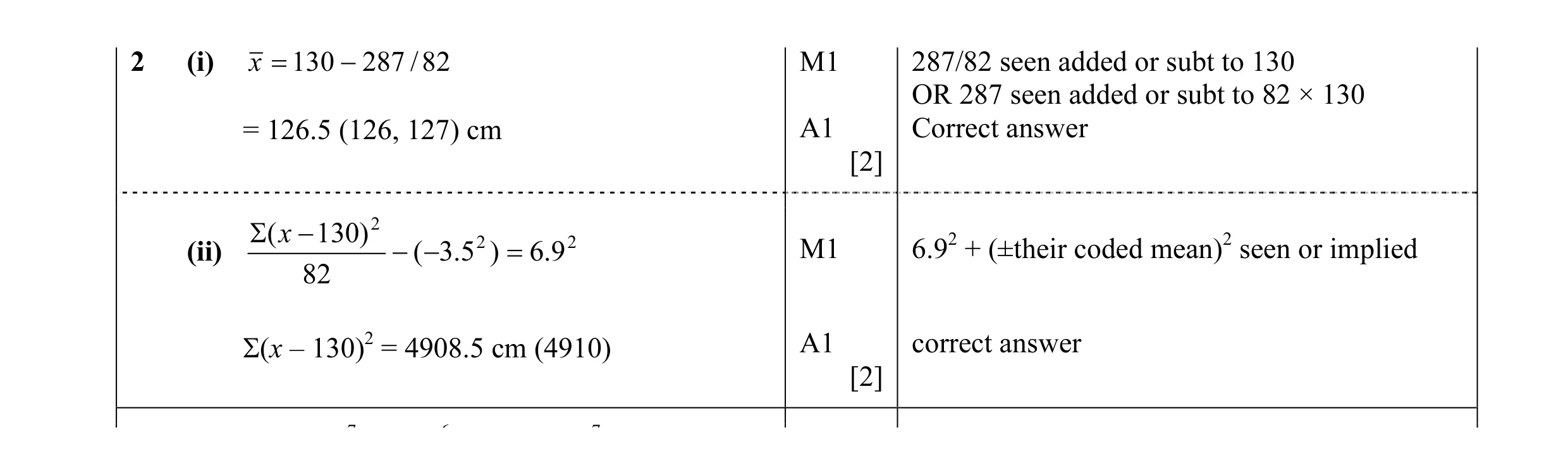 4
4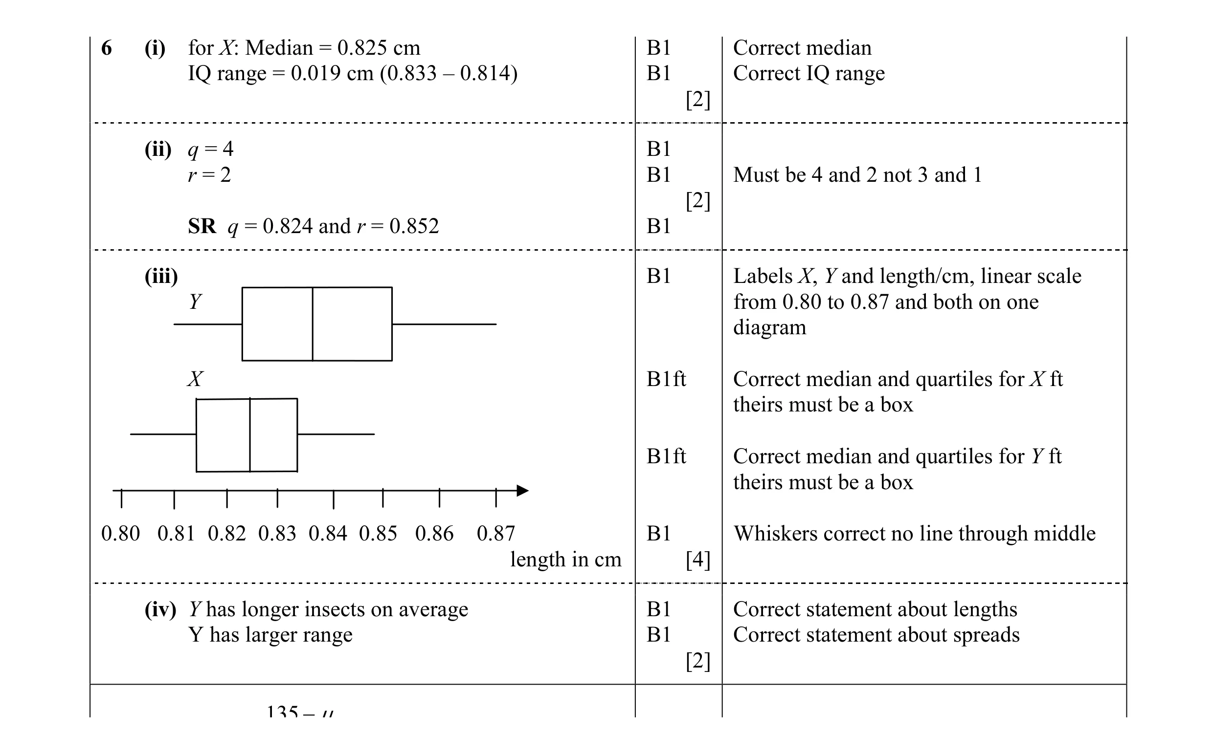 10
10 3
3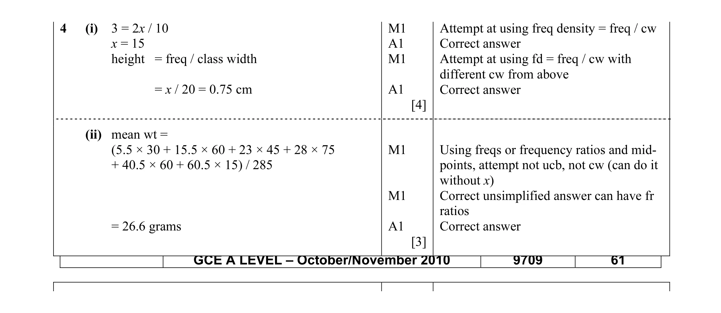 7
7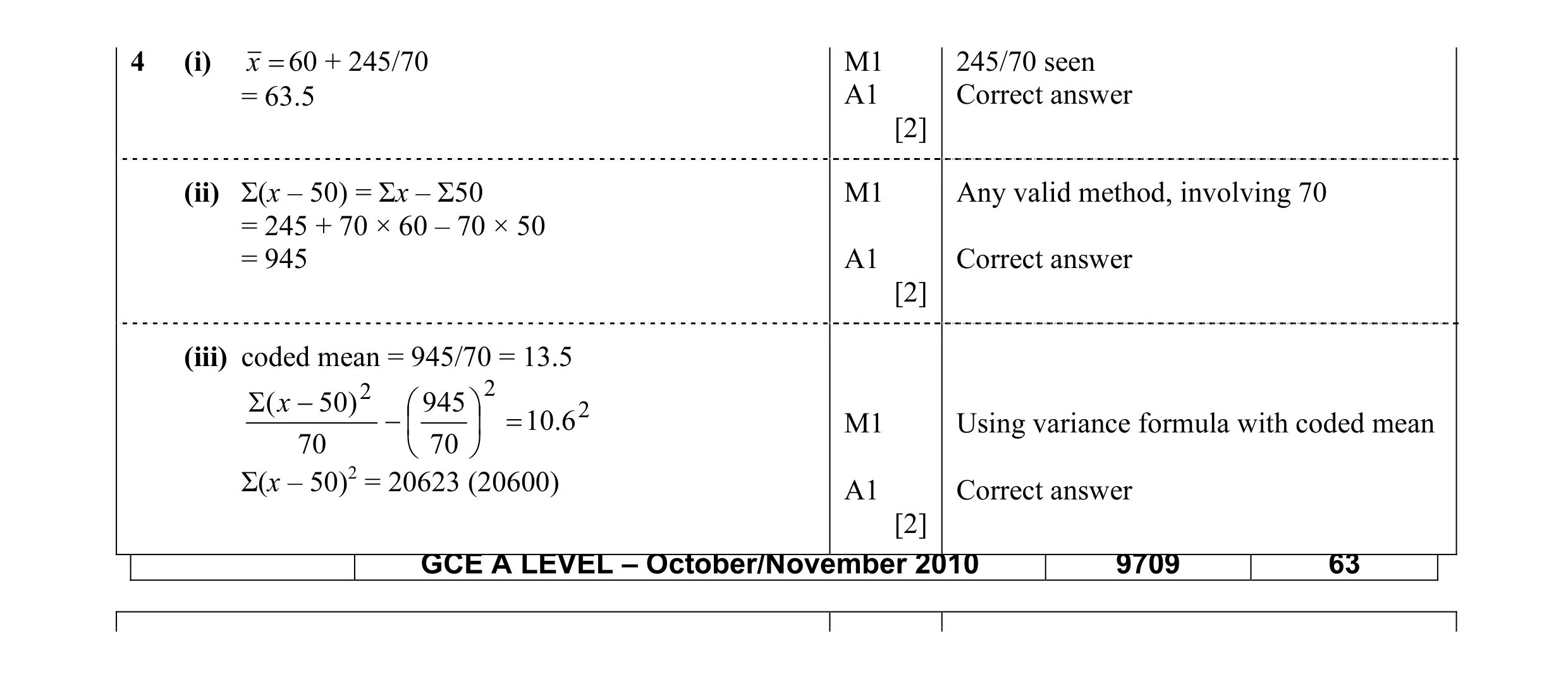 6
6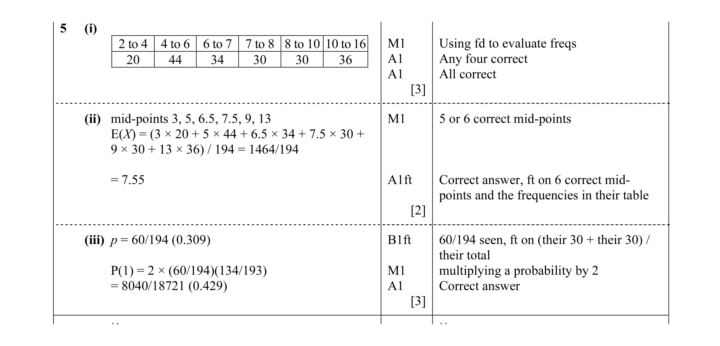 8
8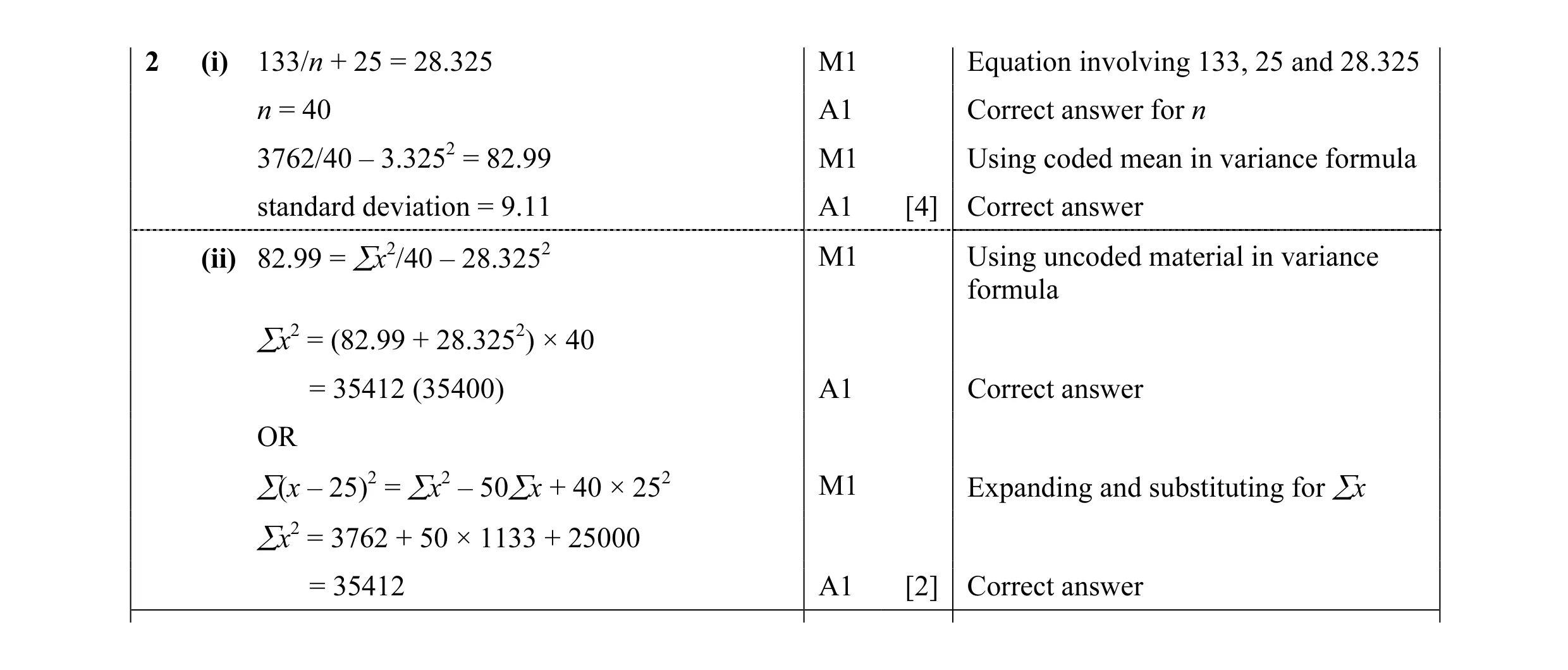 6
6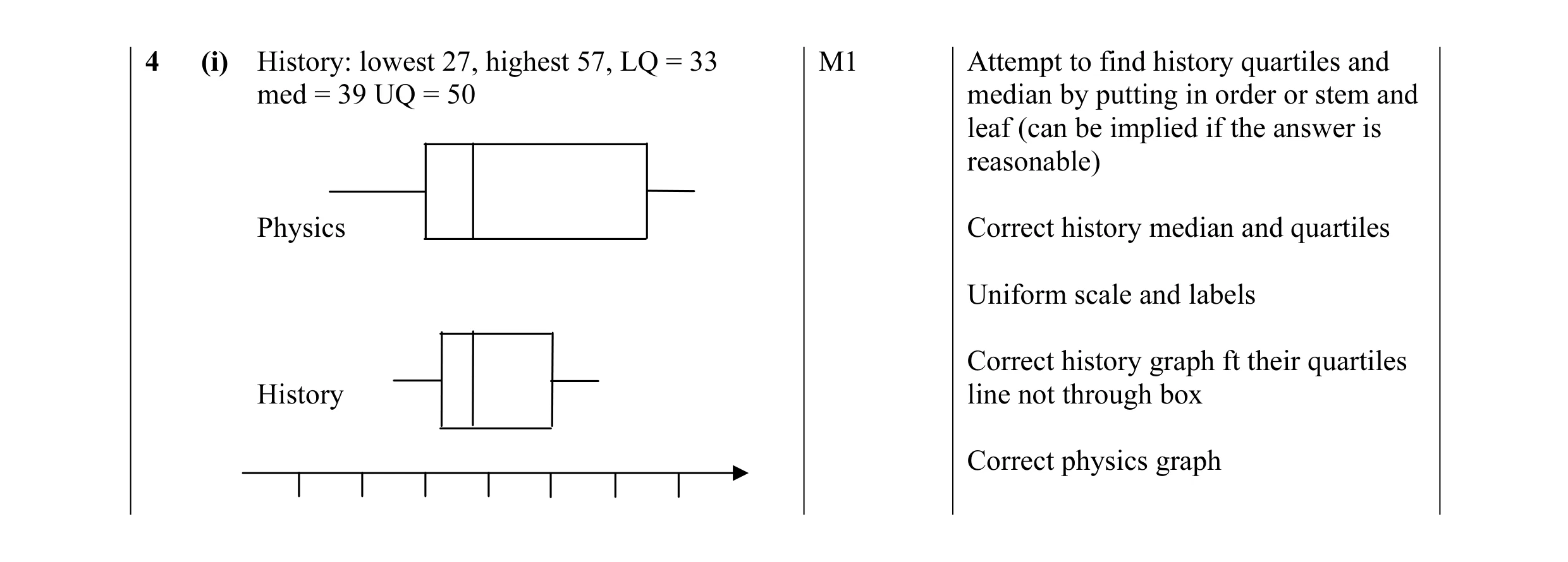 6
6 3
3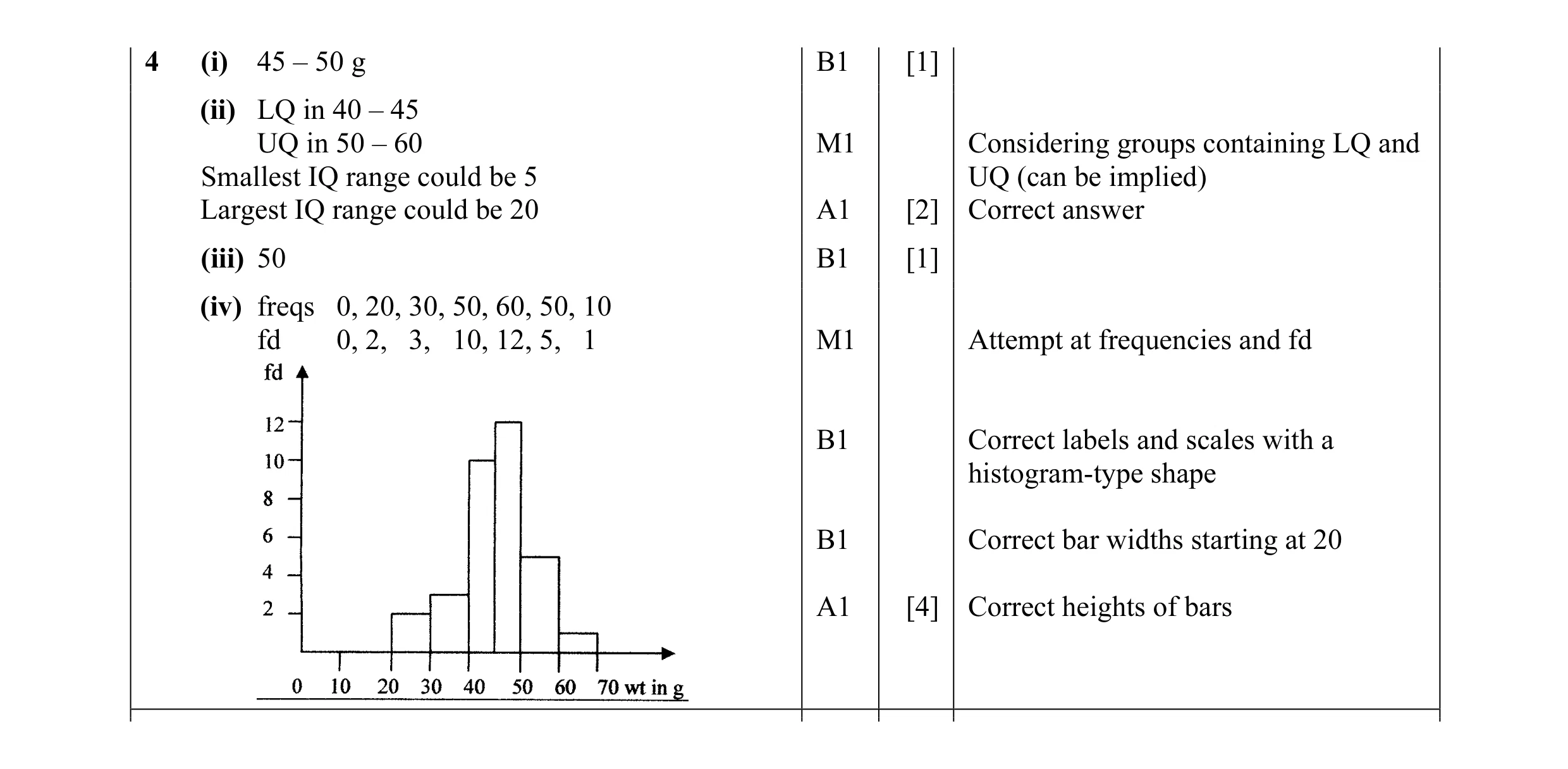 8
8 9
9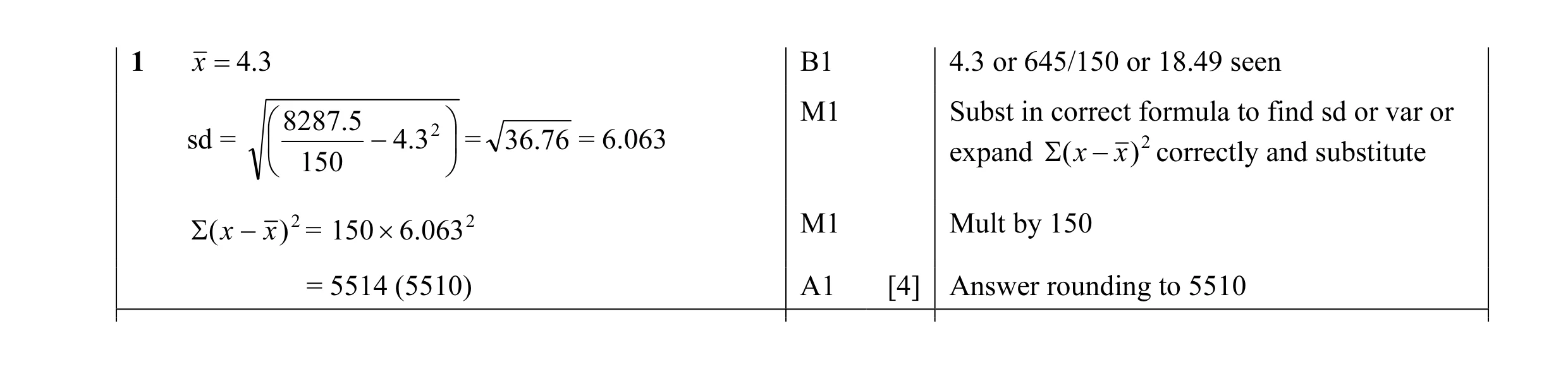 4
4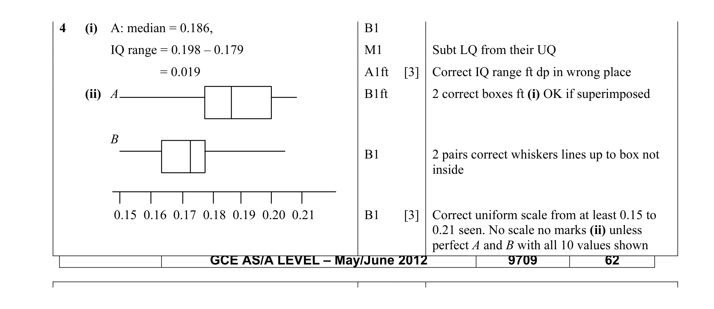 6
6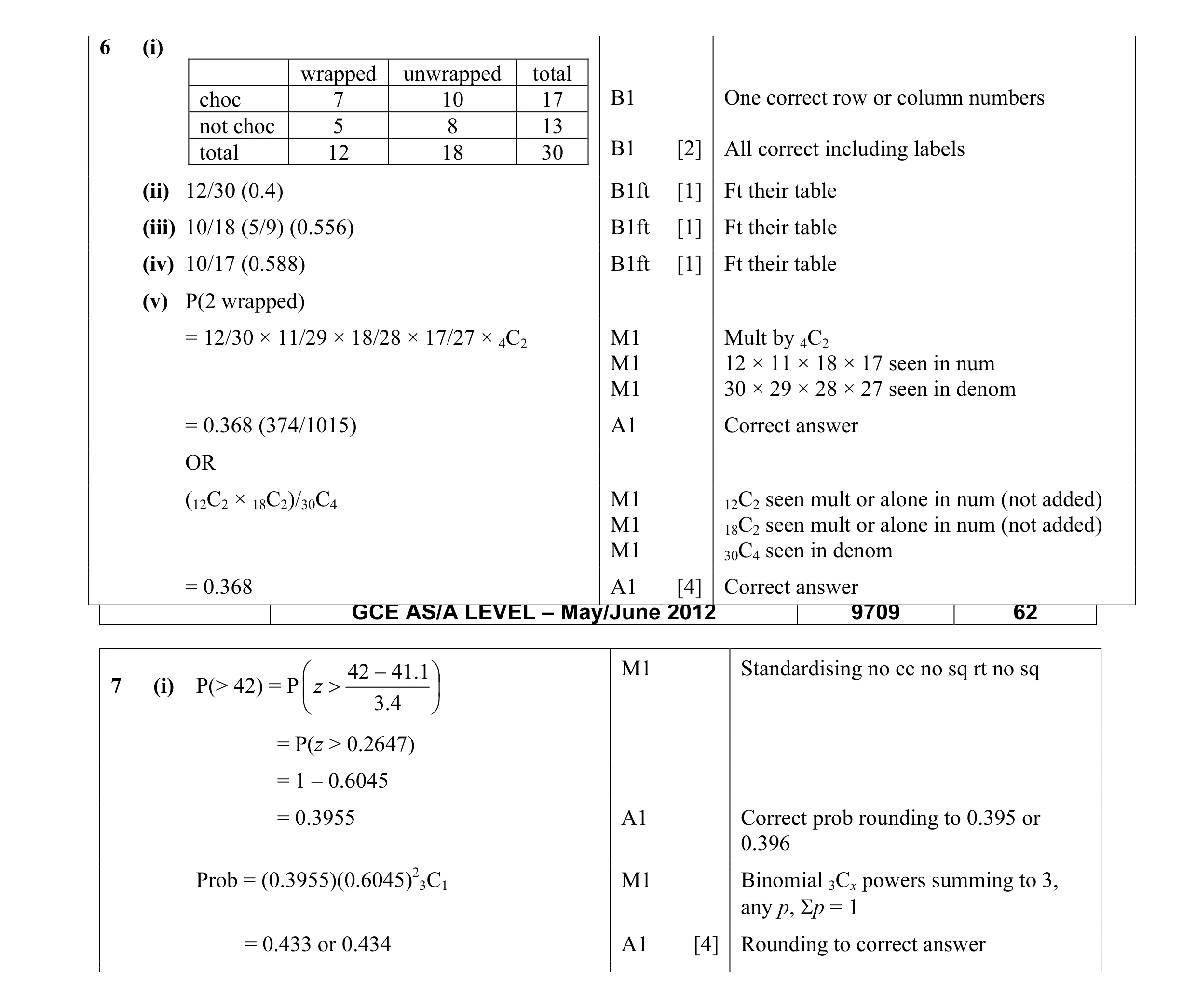 9
9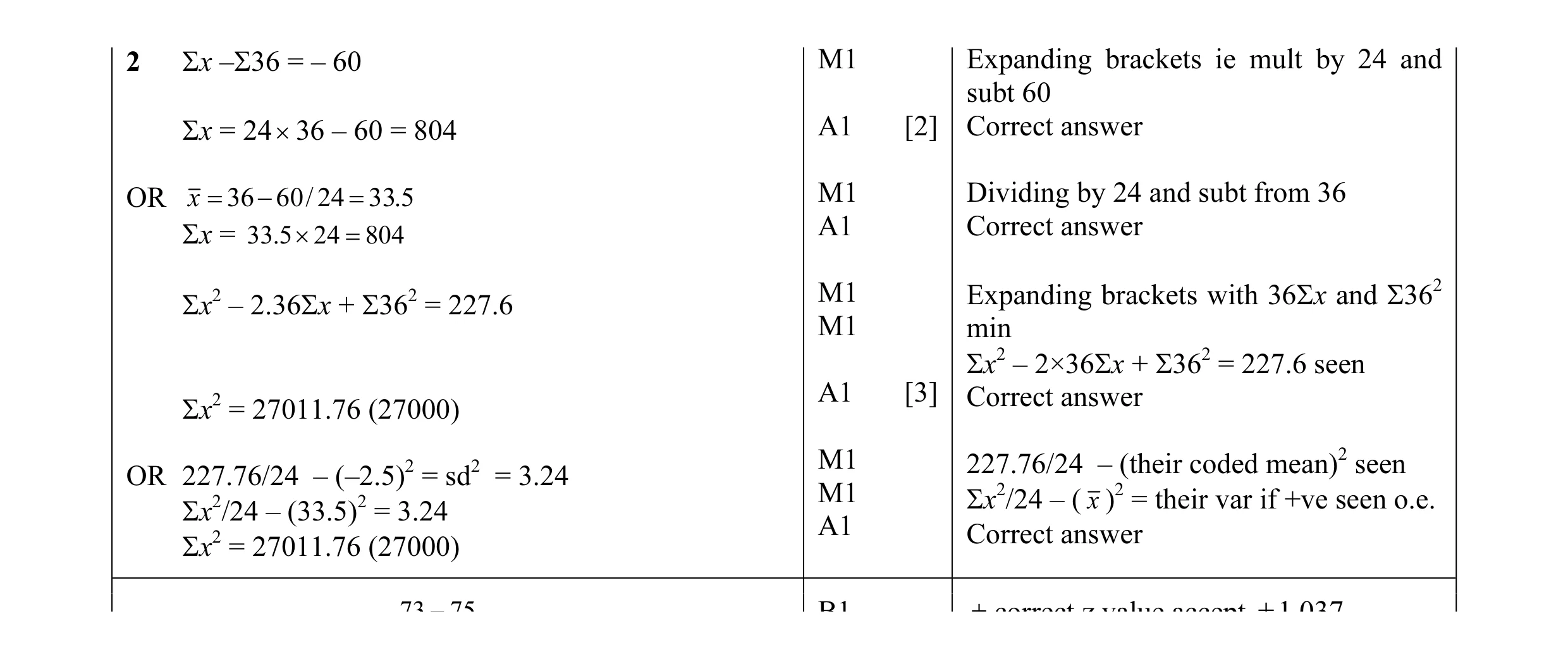 5
5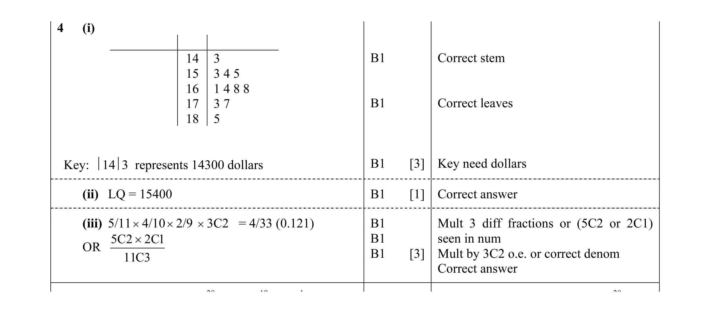 7
7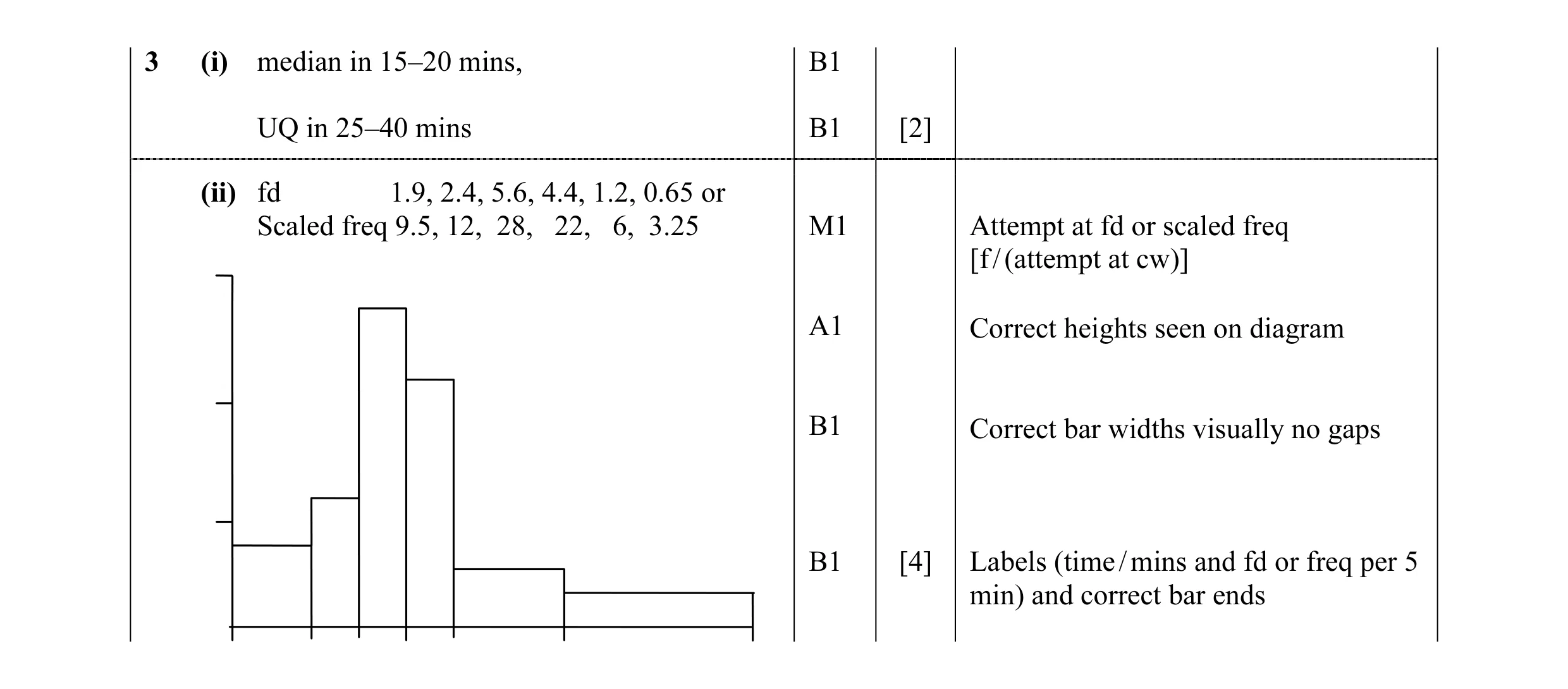 8
8 4
4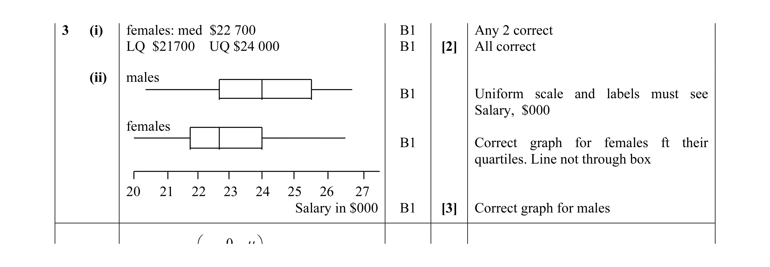 5
5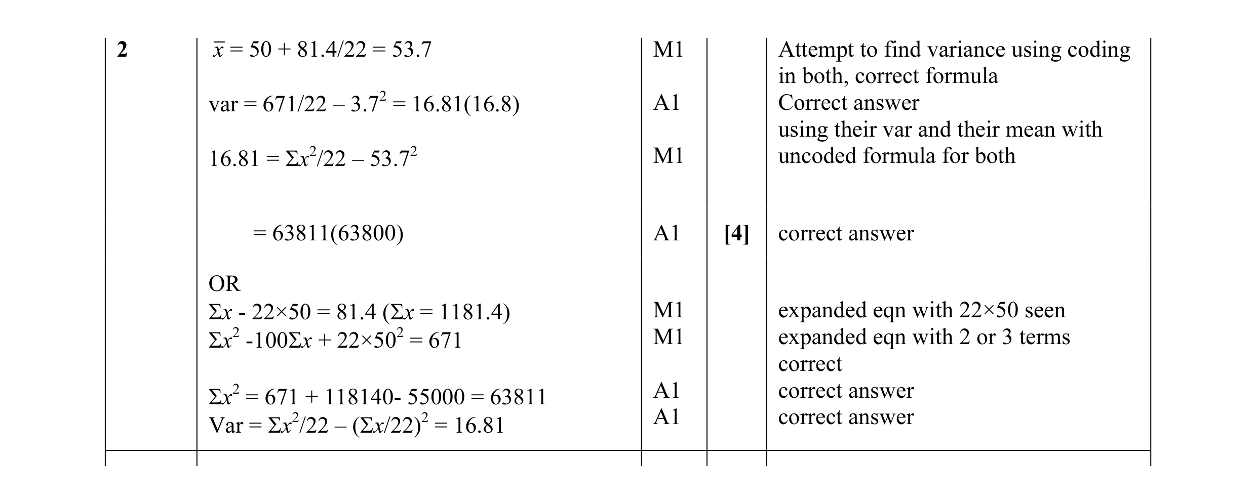 4
4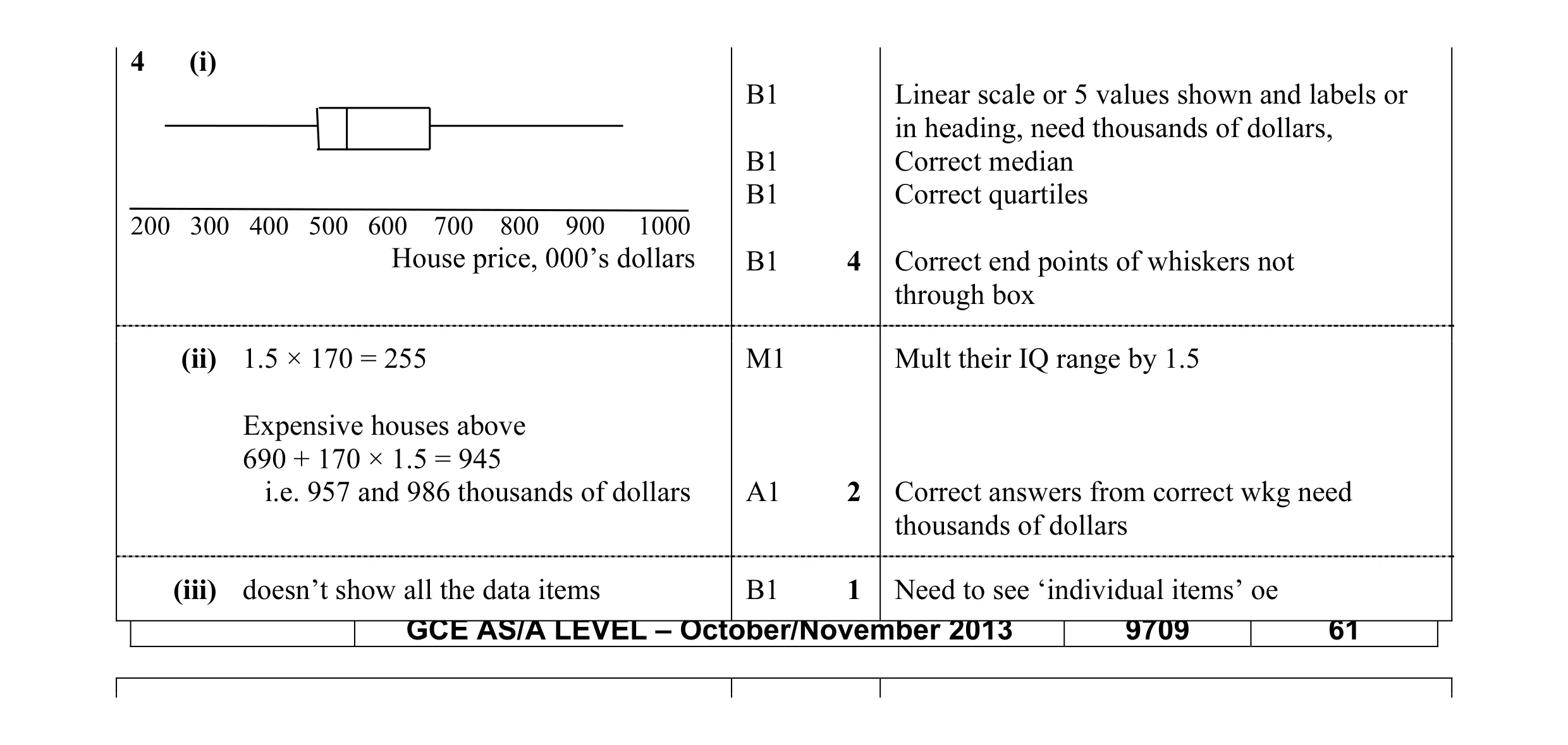 7
7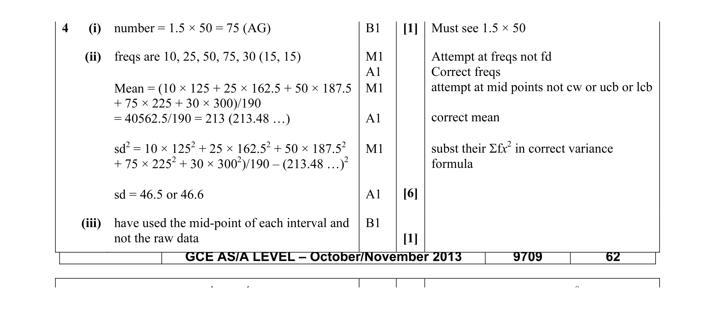 8
8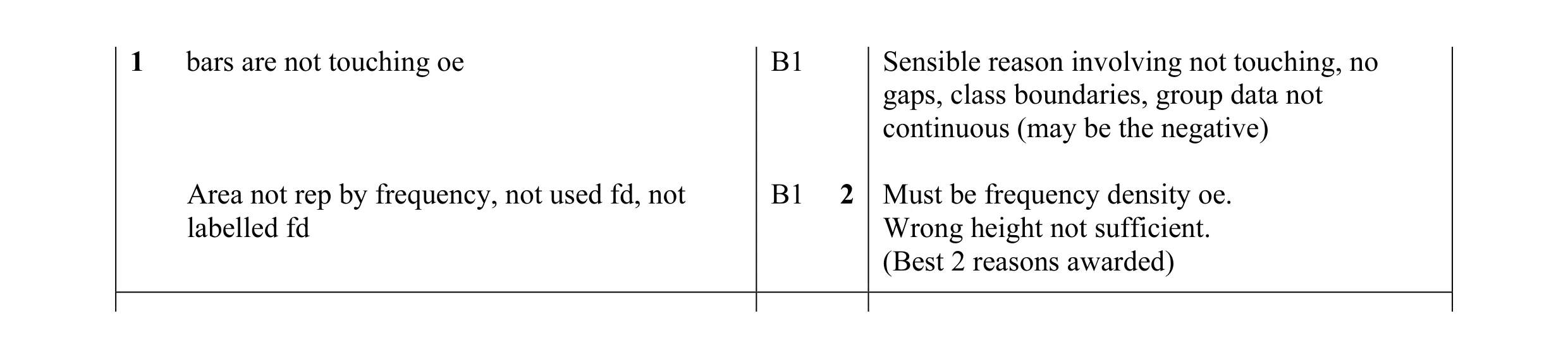 2
2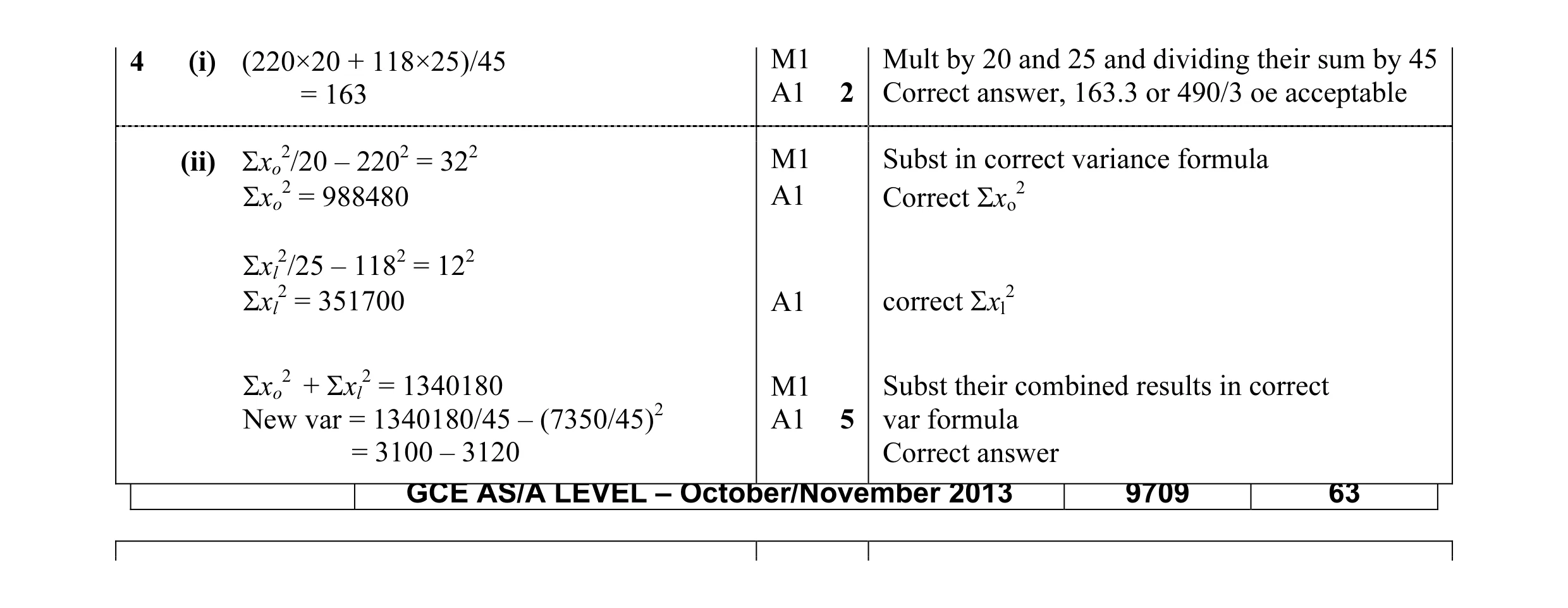 7
7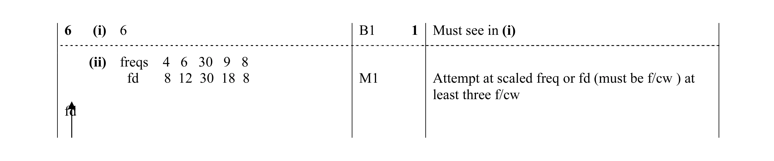 9
9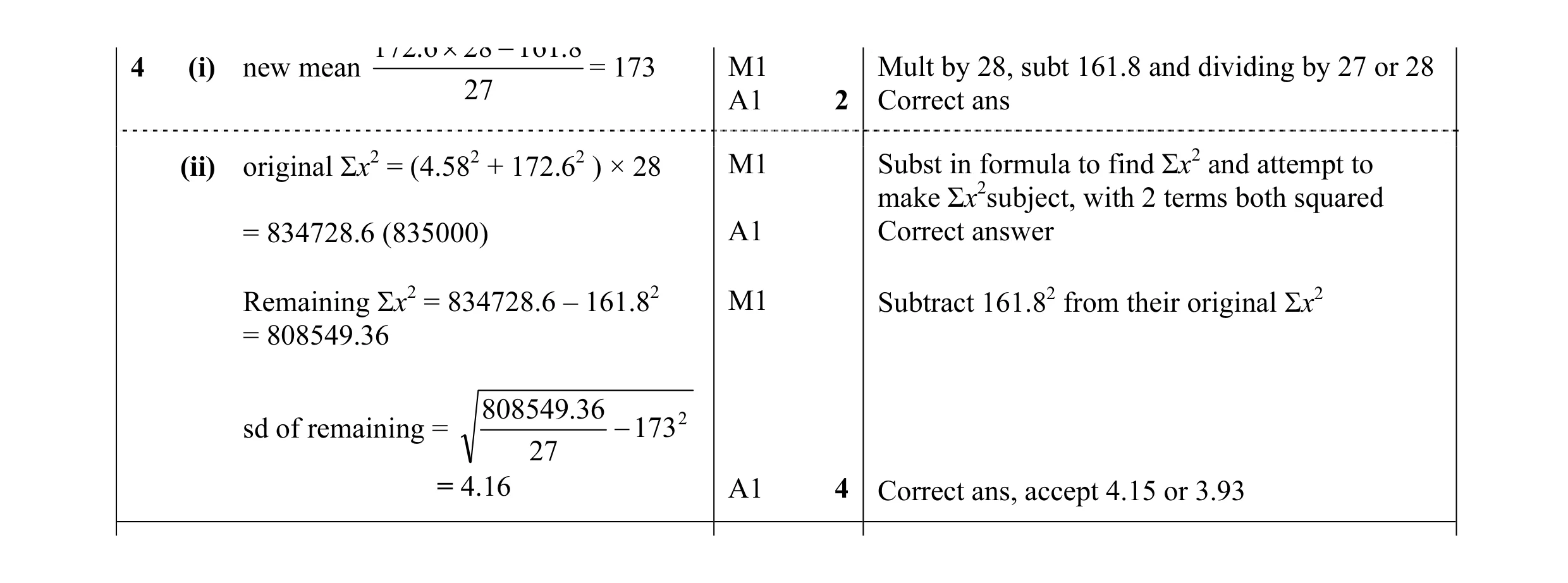 6
6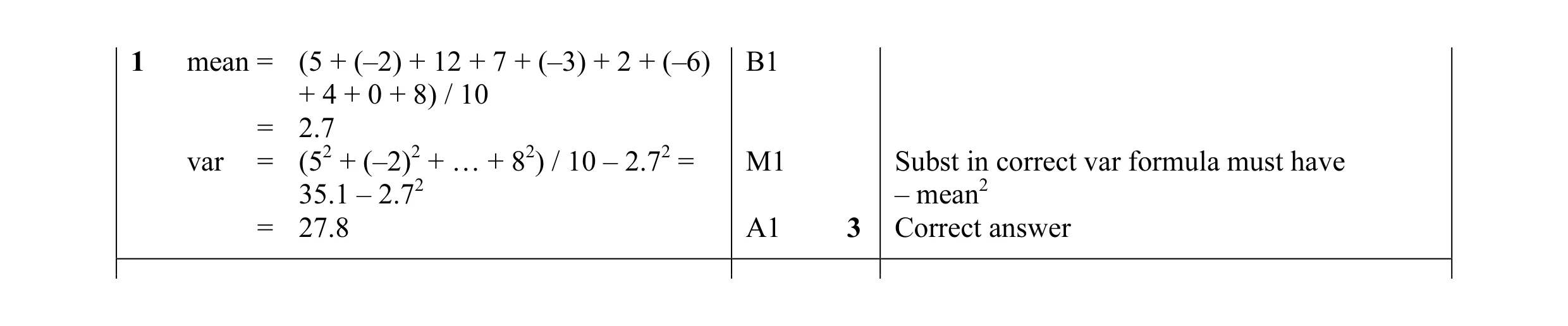 3
3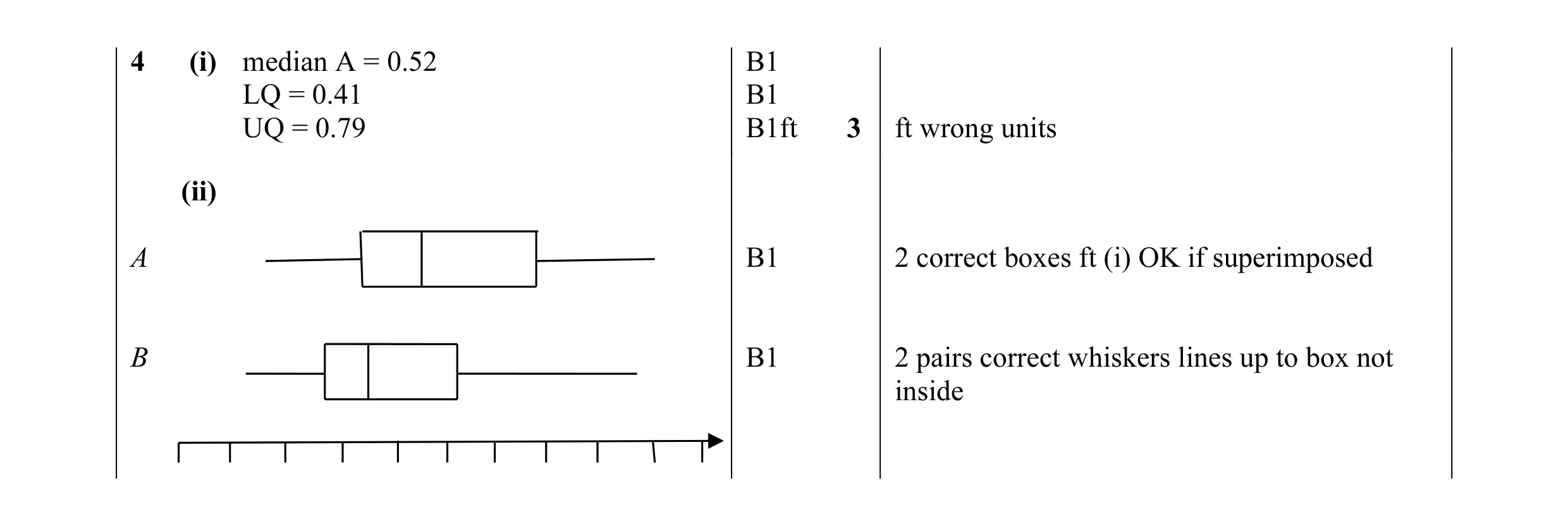 7
7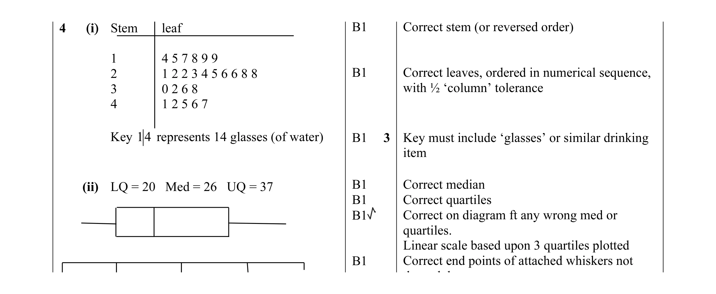 8
8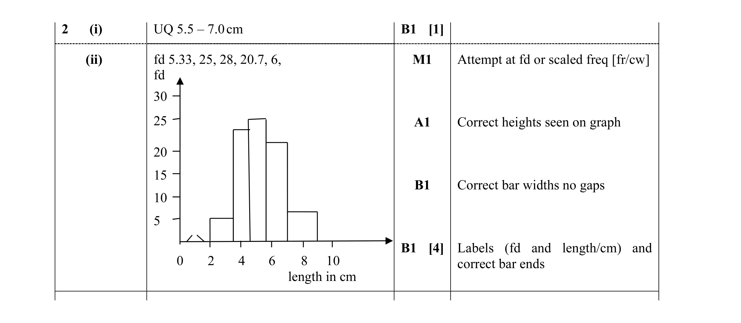 5
5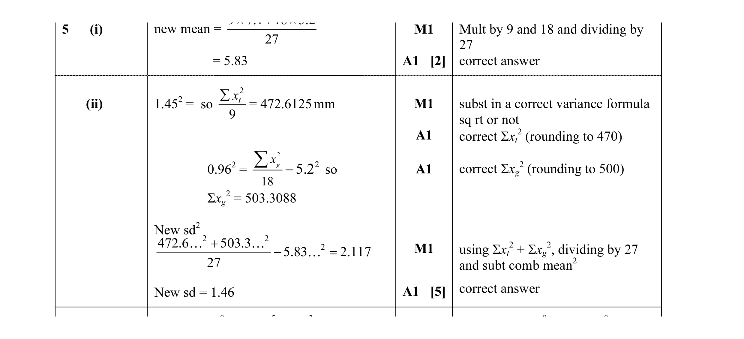 7
7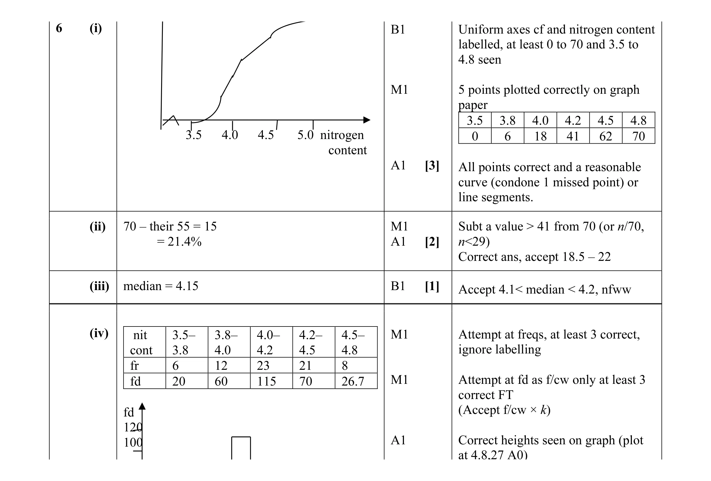 11
11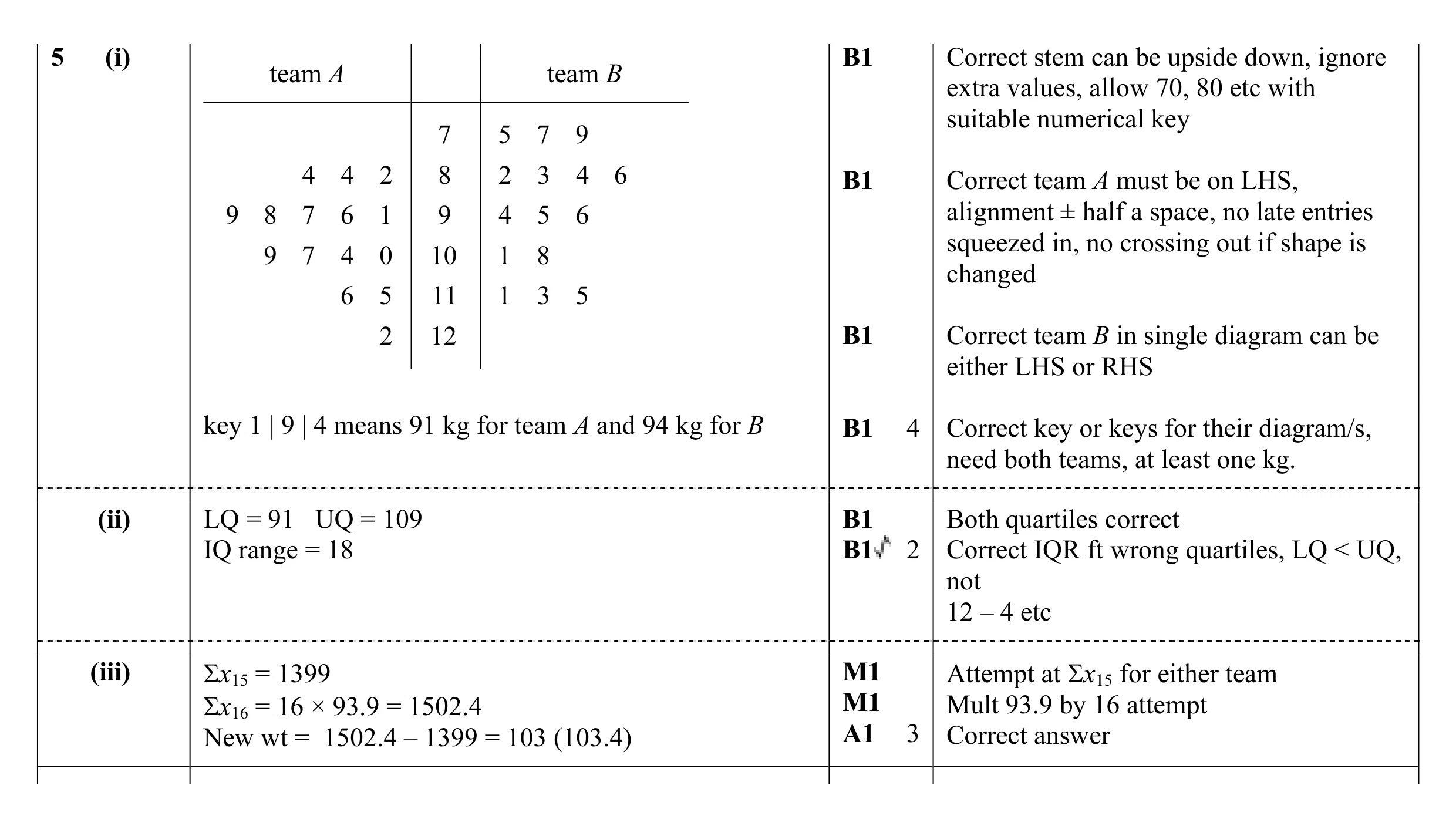 9
9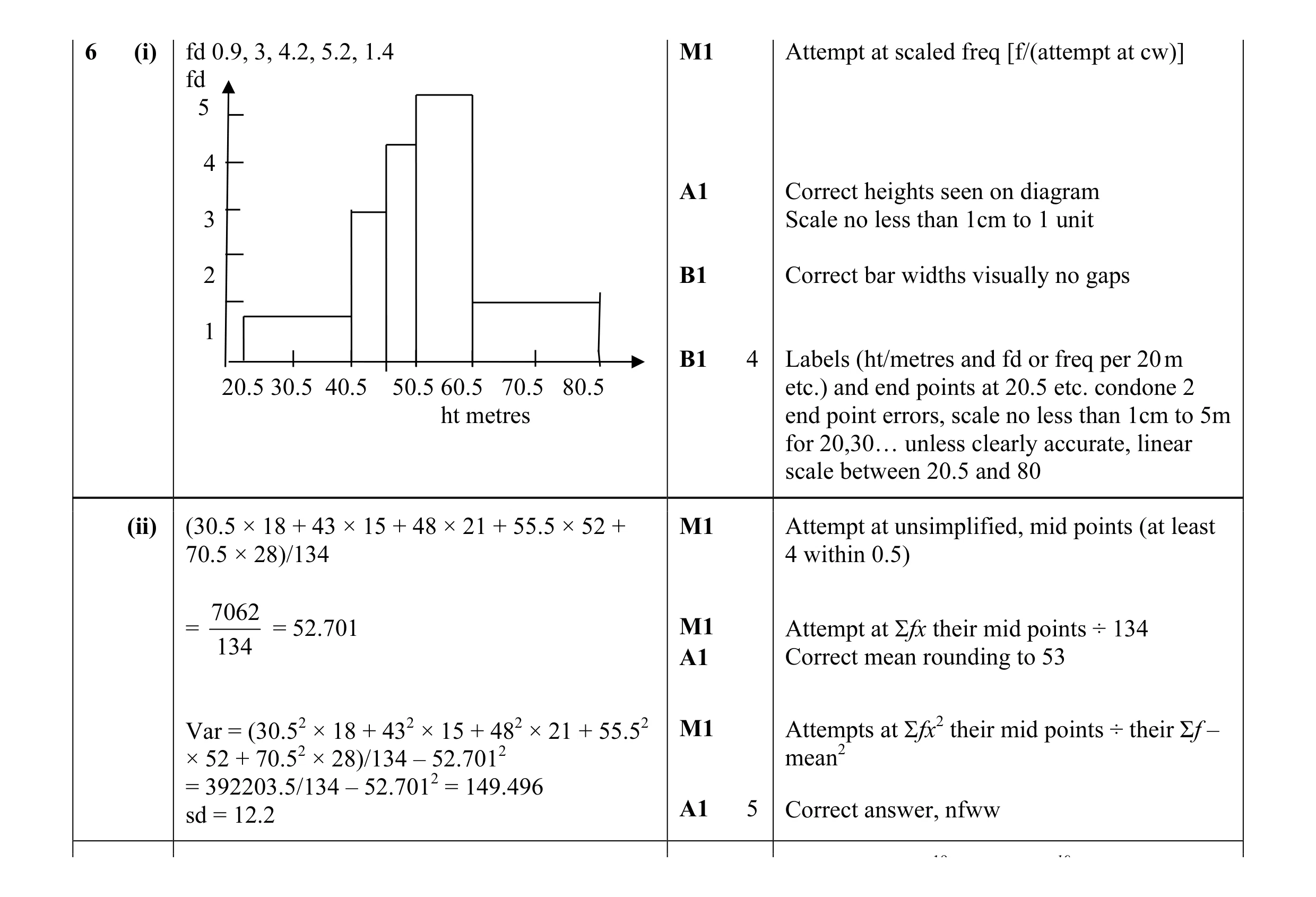 9
9 3
3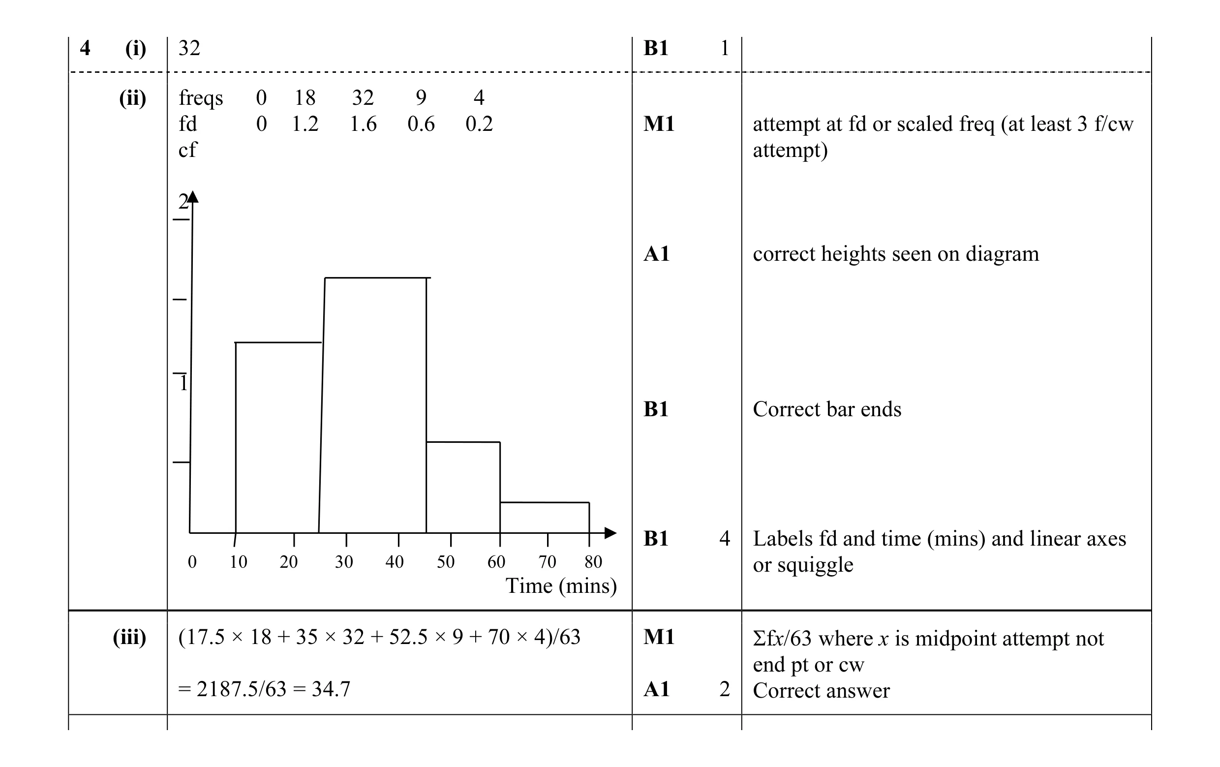 7
7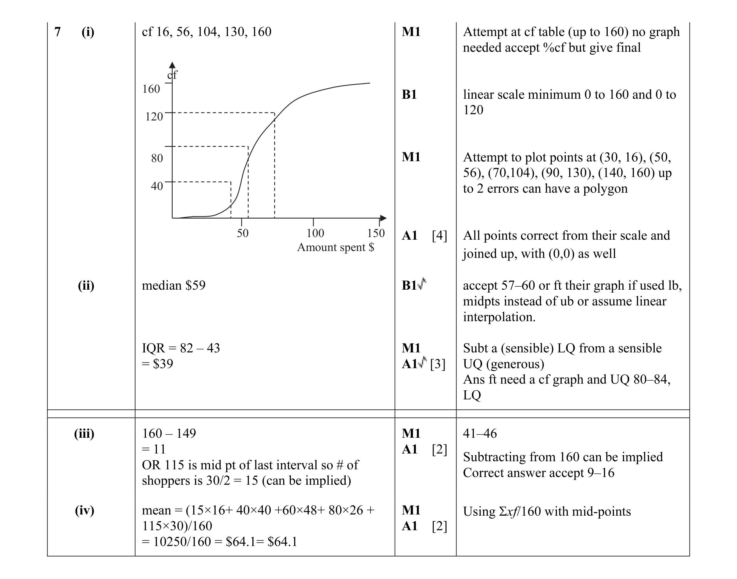 11
11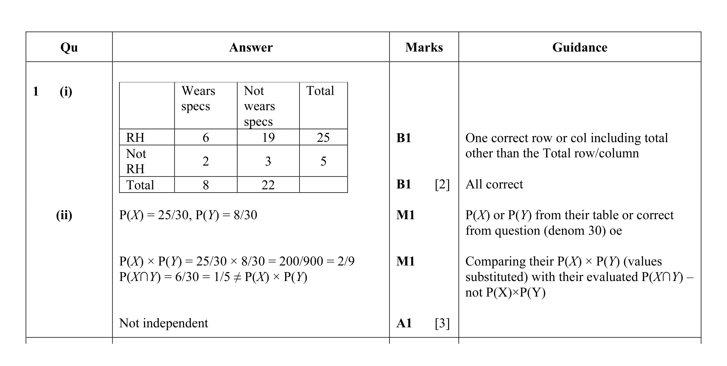 5
5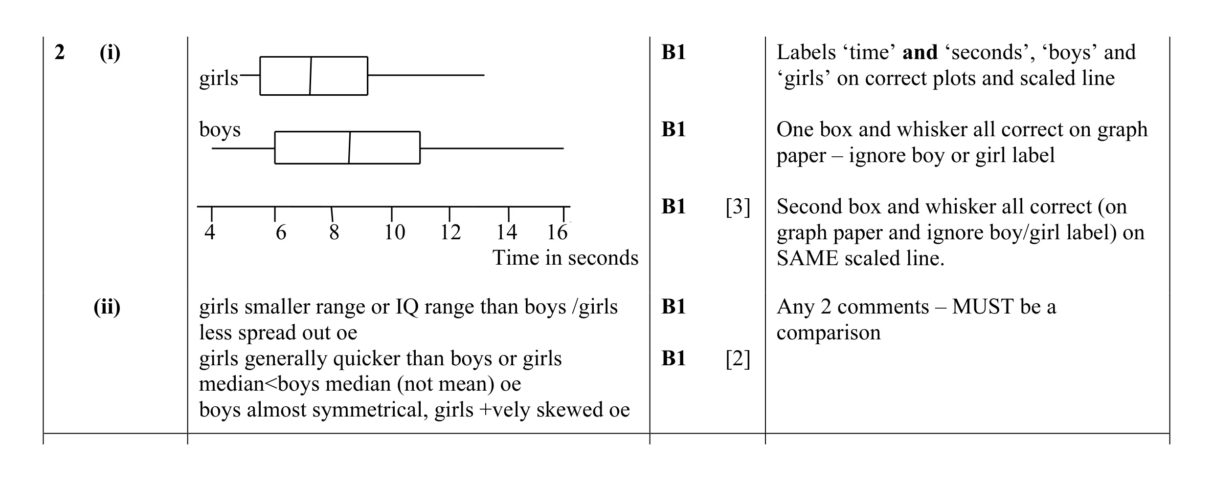 5
5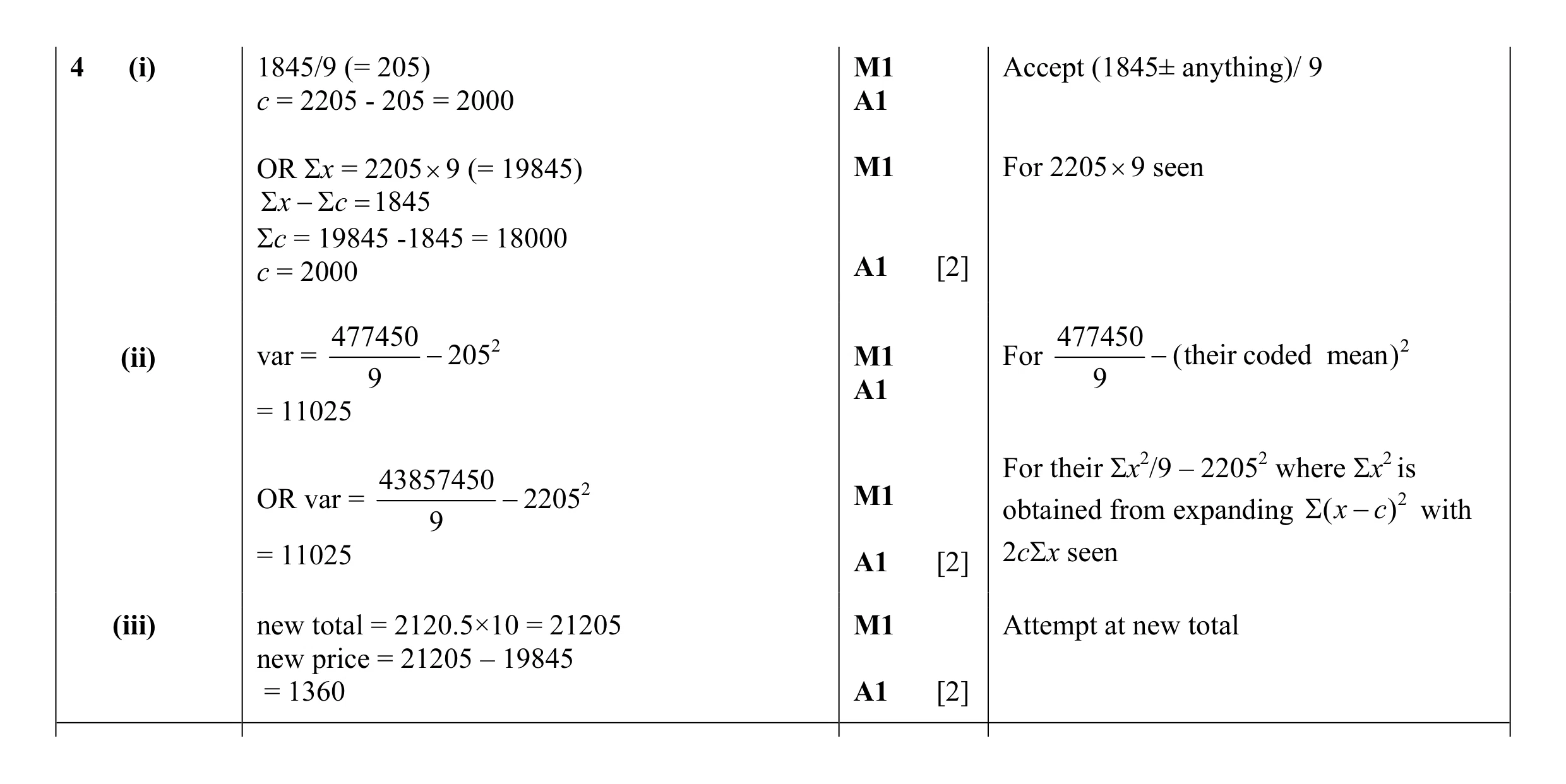 6
6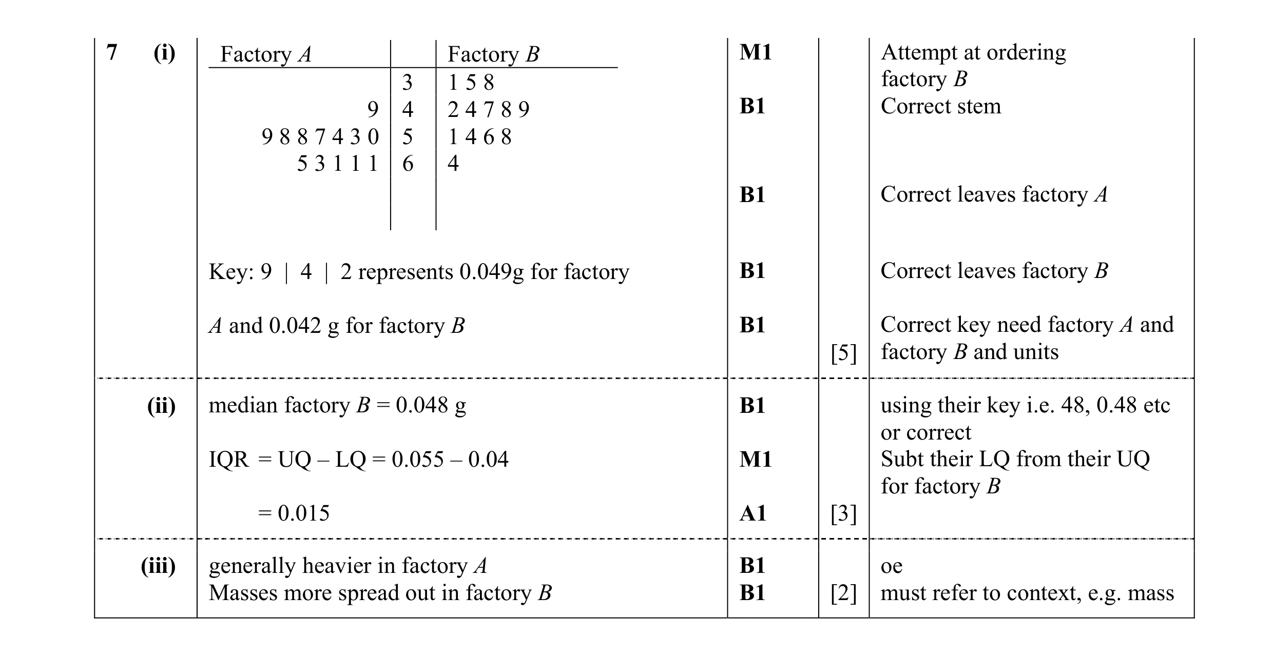 10
10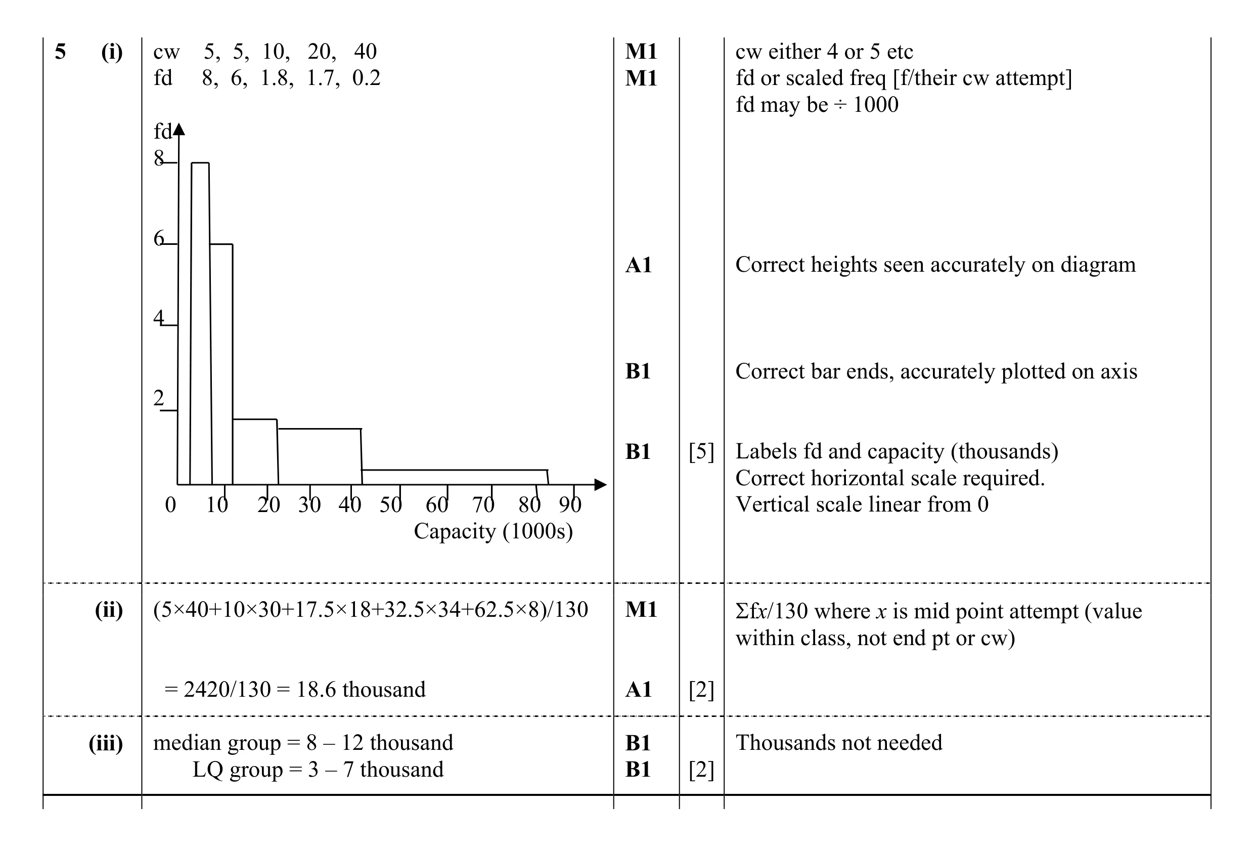 9
9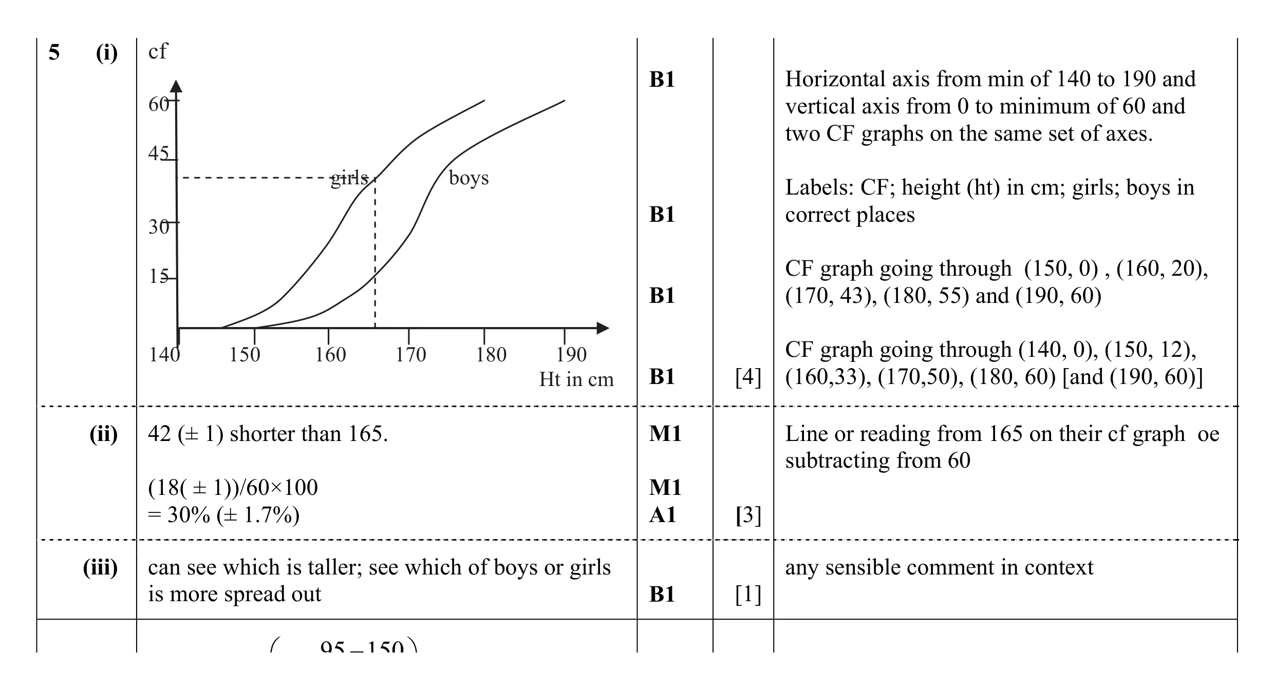 8
8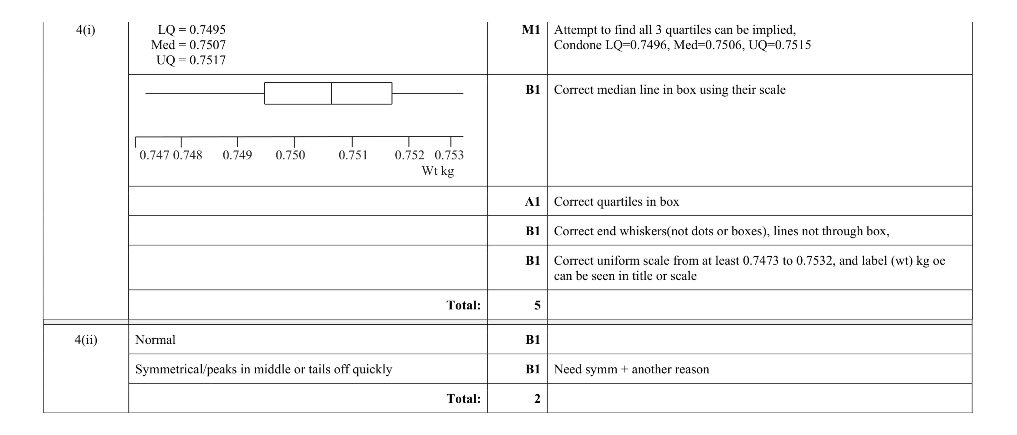 7
7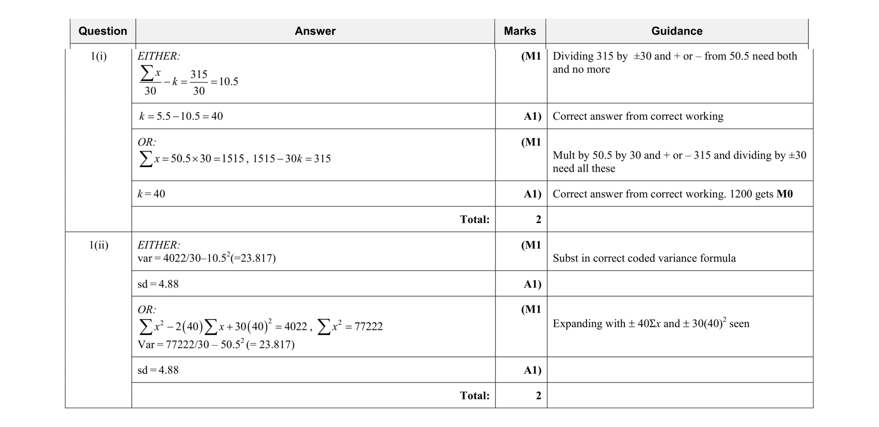 4
4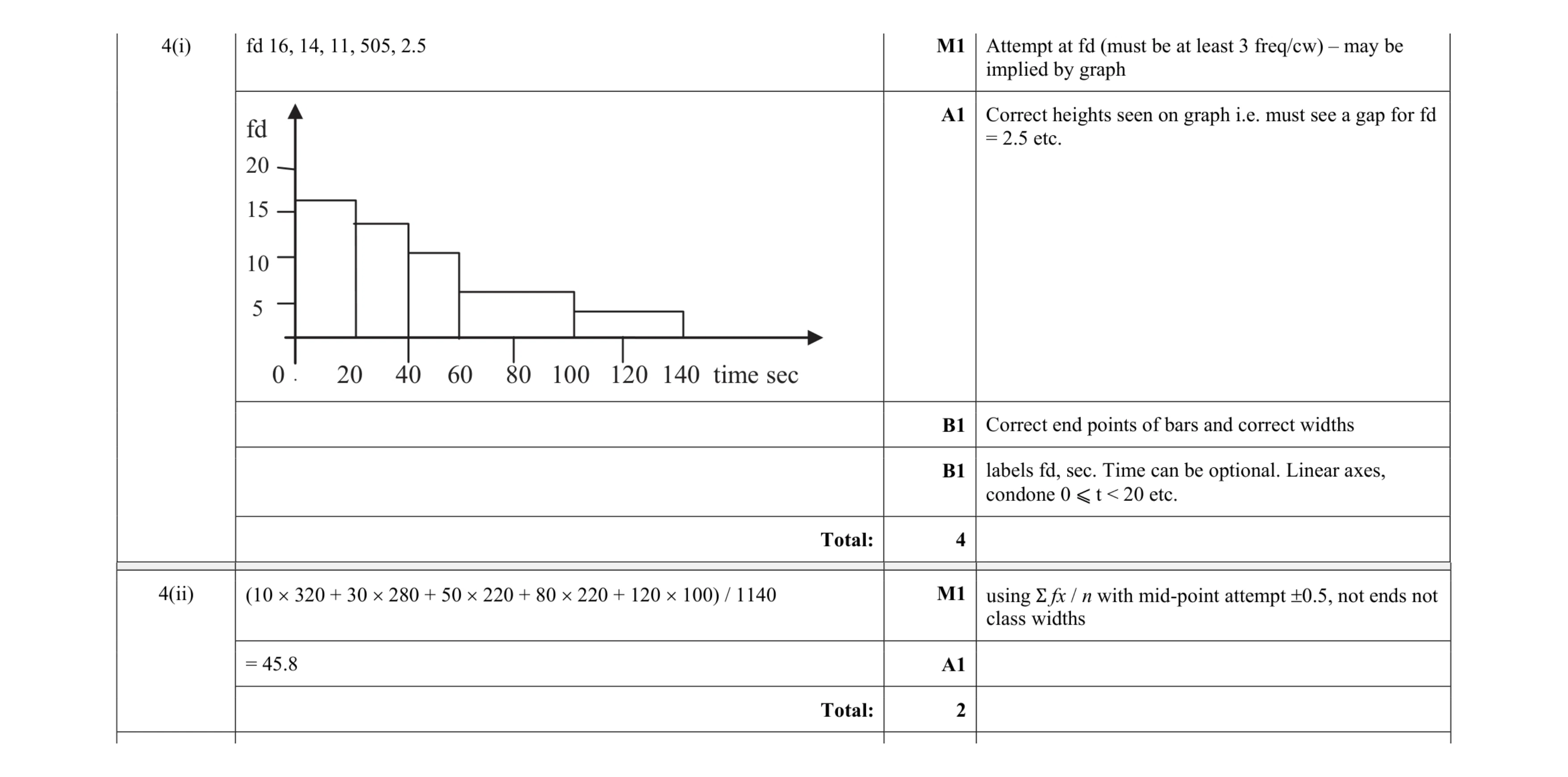 6
6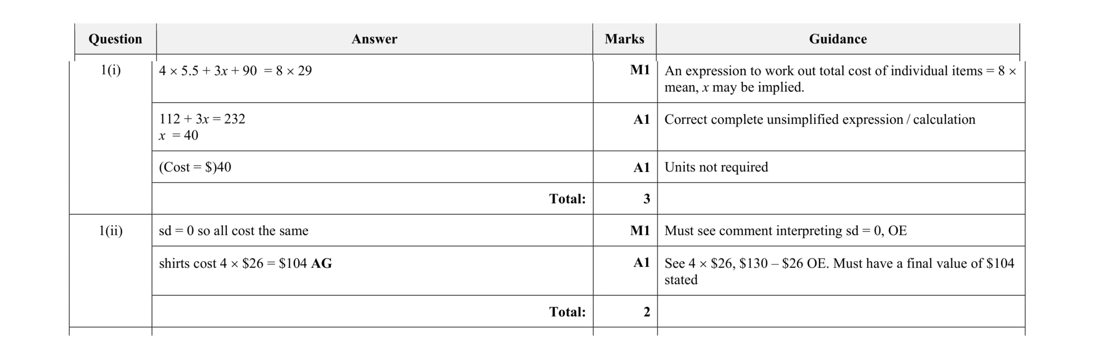 5
5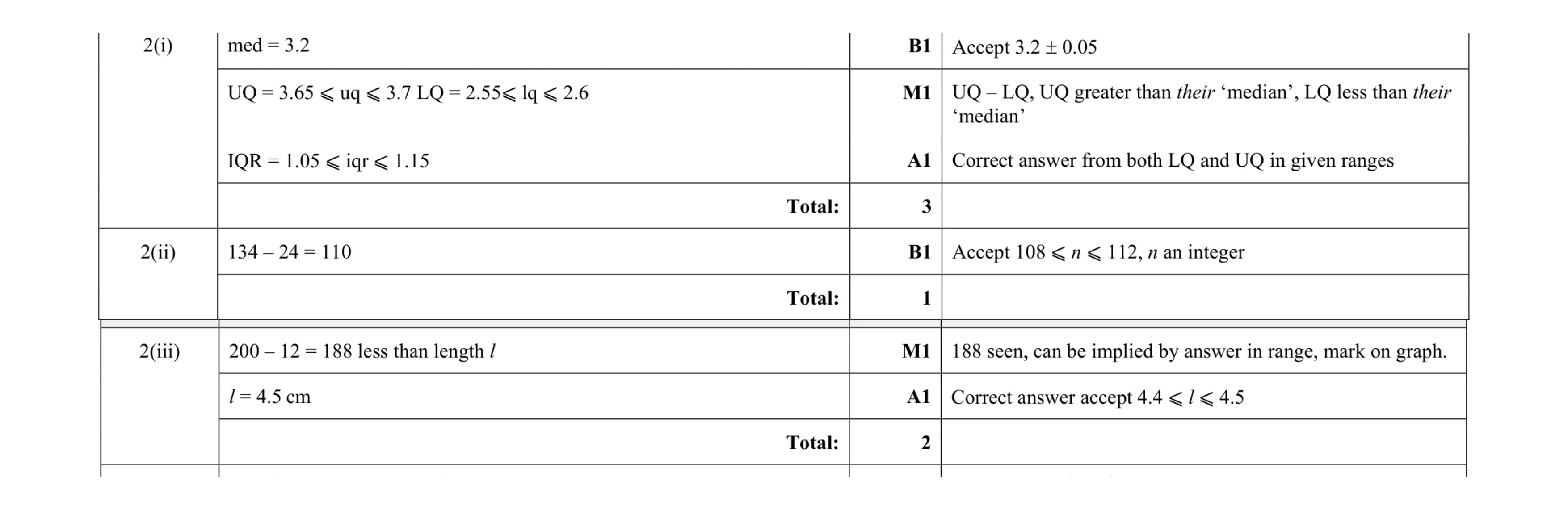 6
6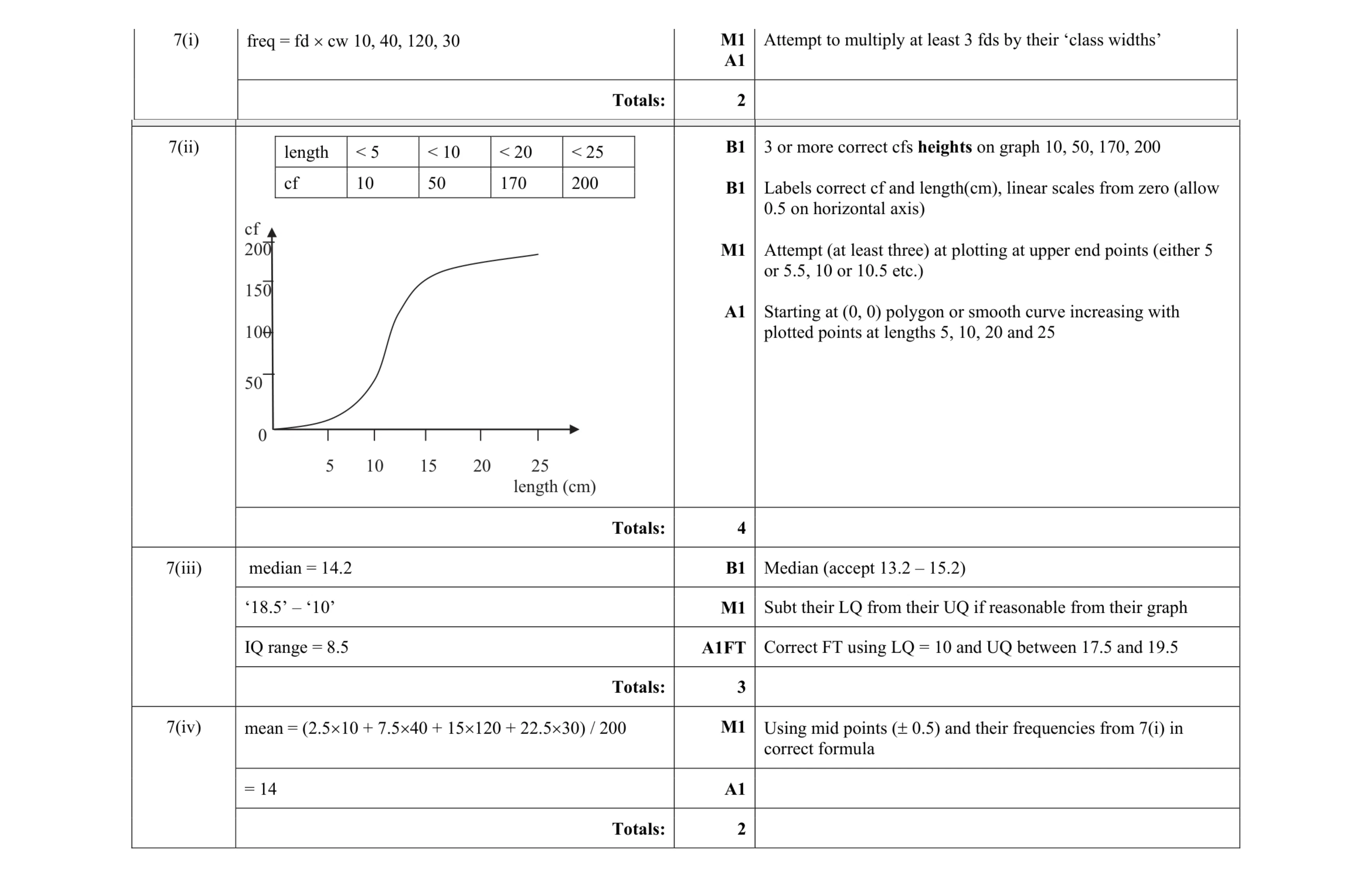 11
11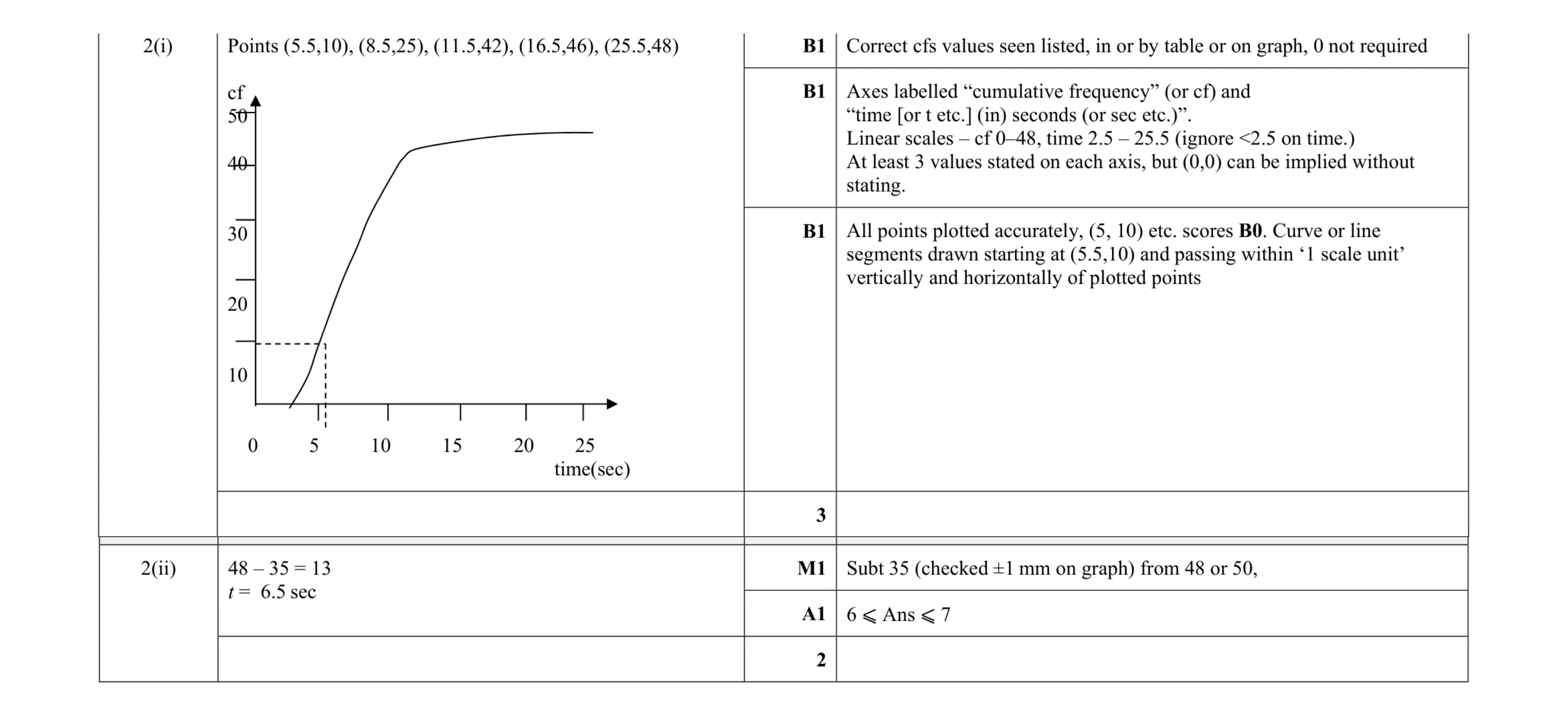 5
5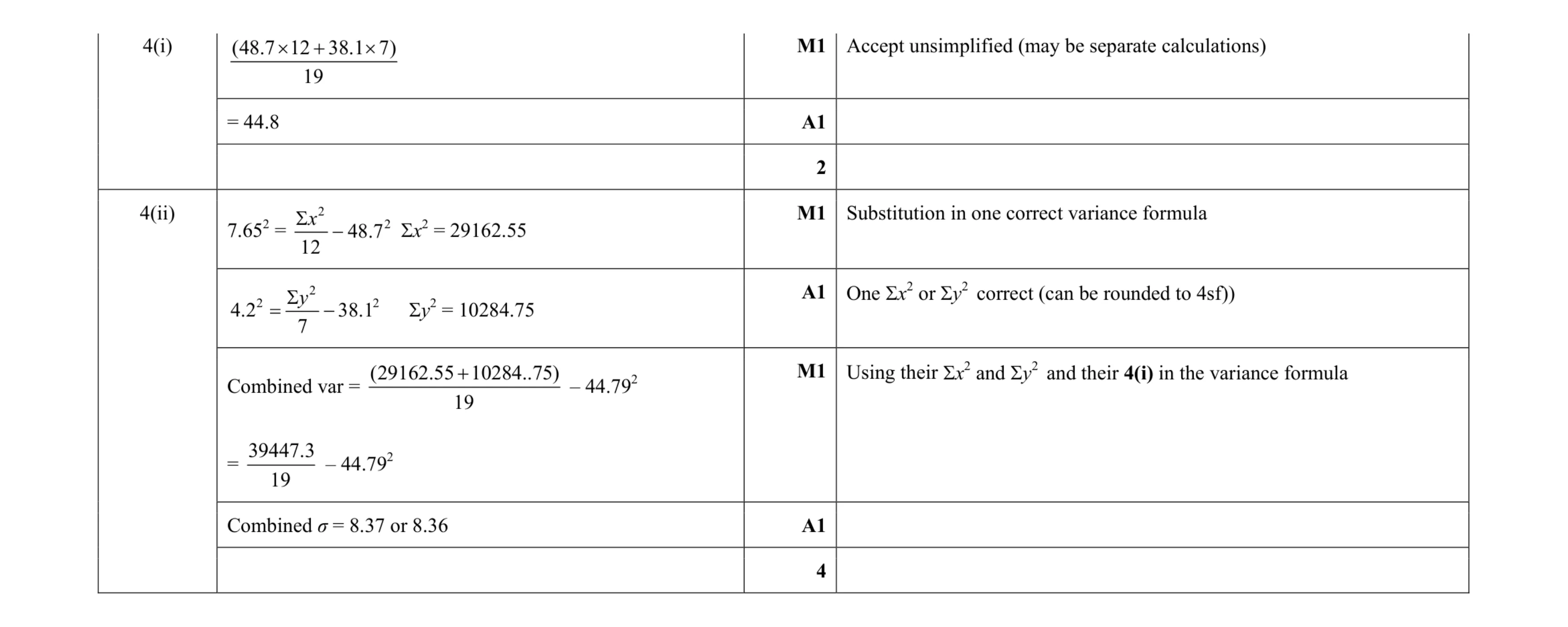 6
6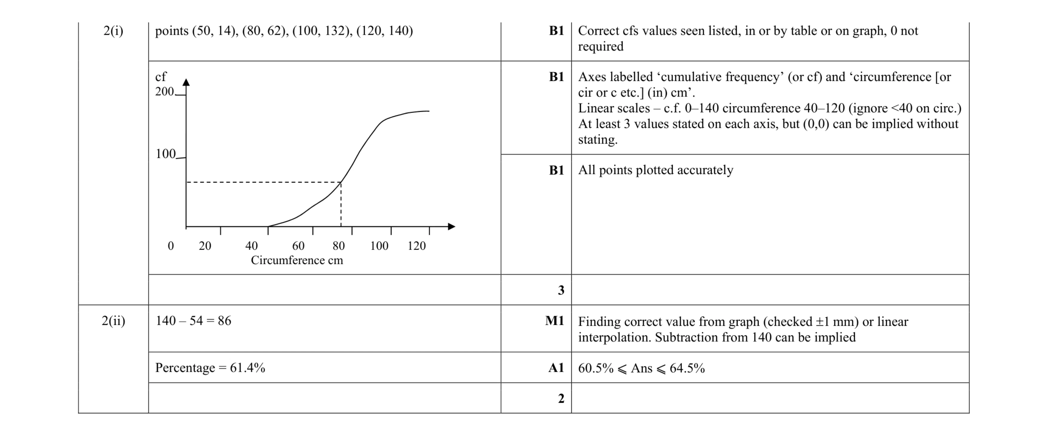 5
5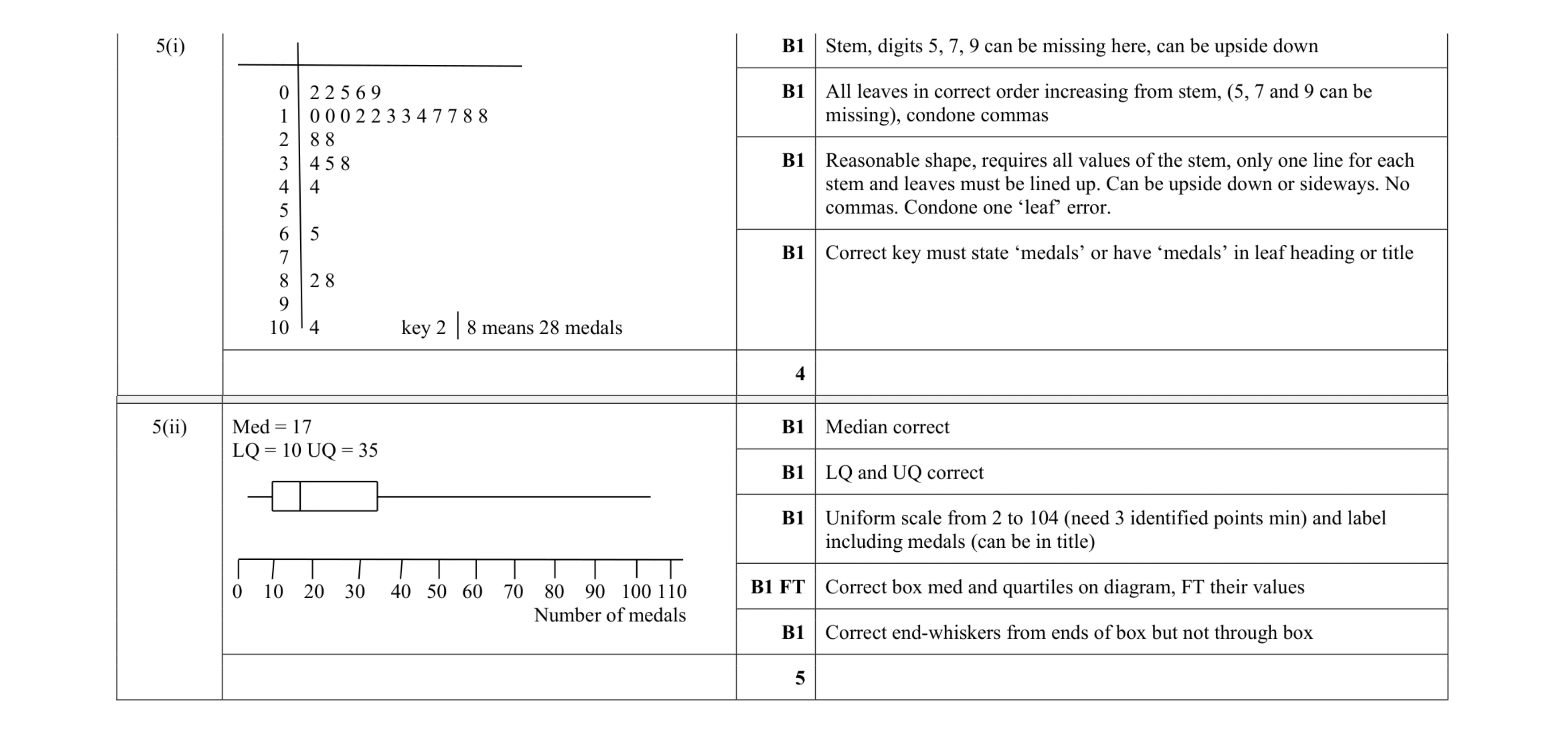 9
9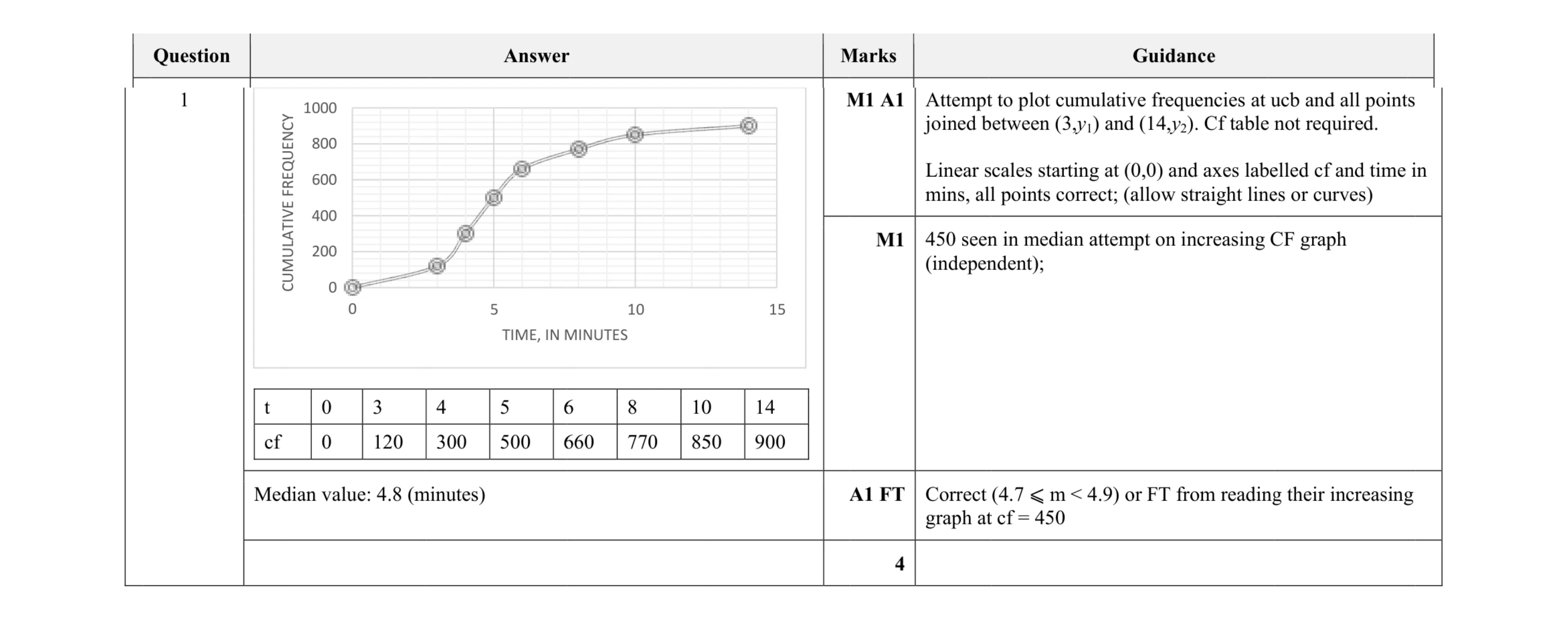 4
4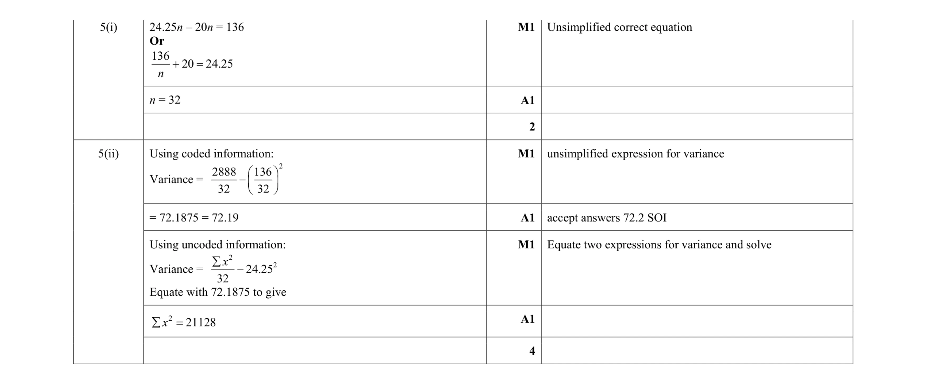 6
6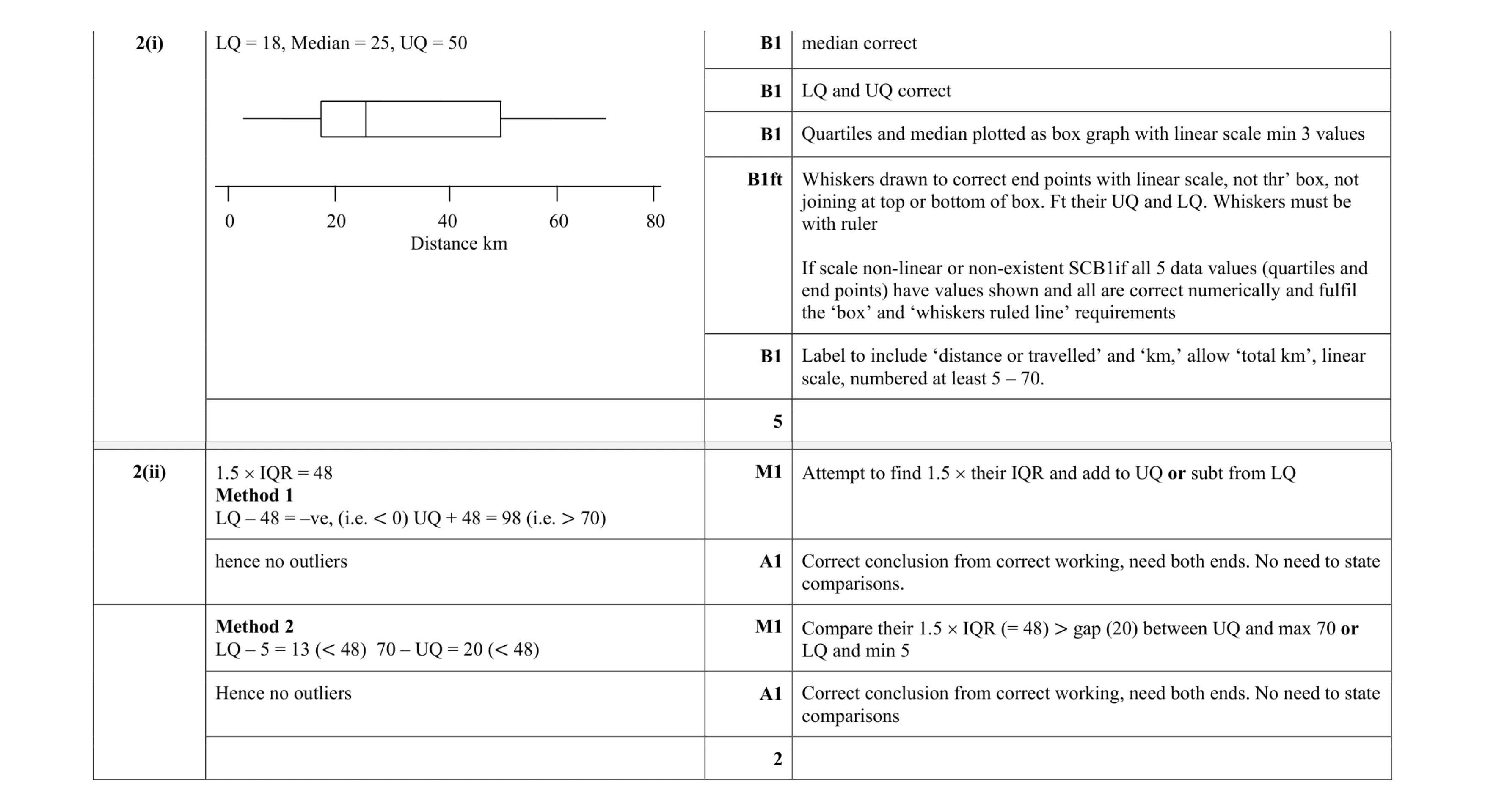 7
7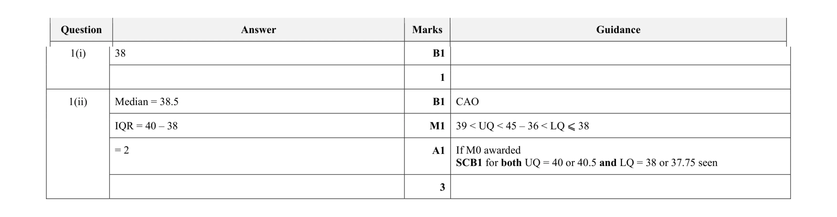 4
4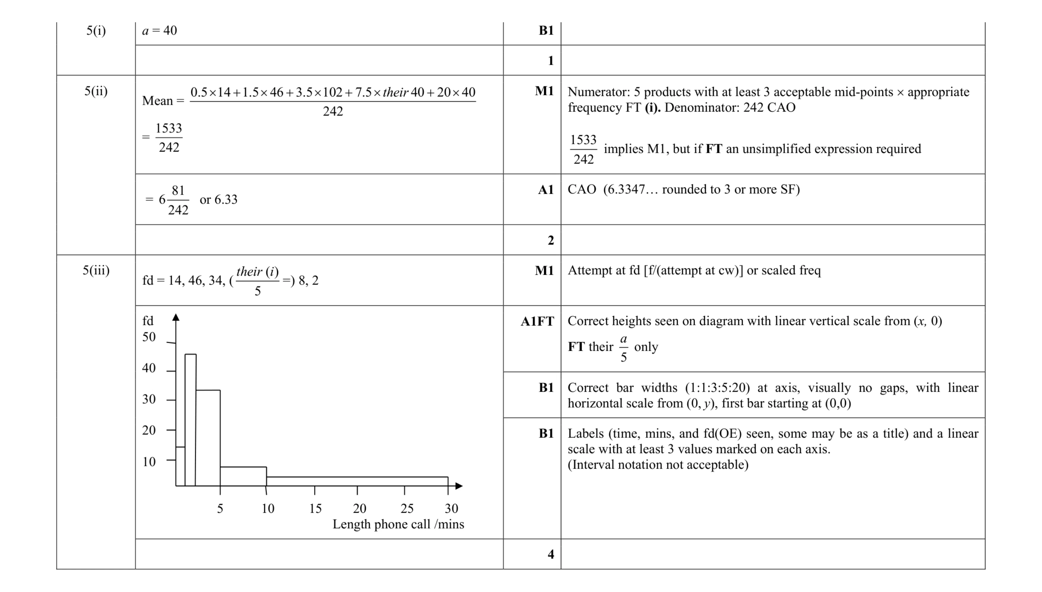 7
7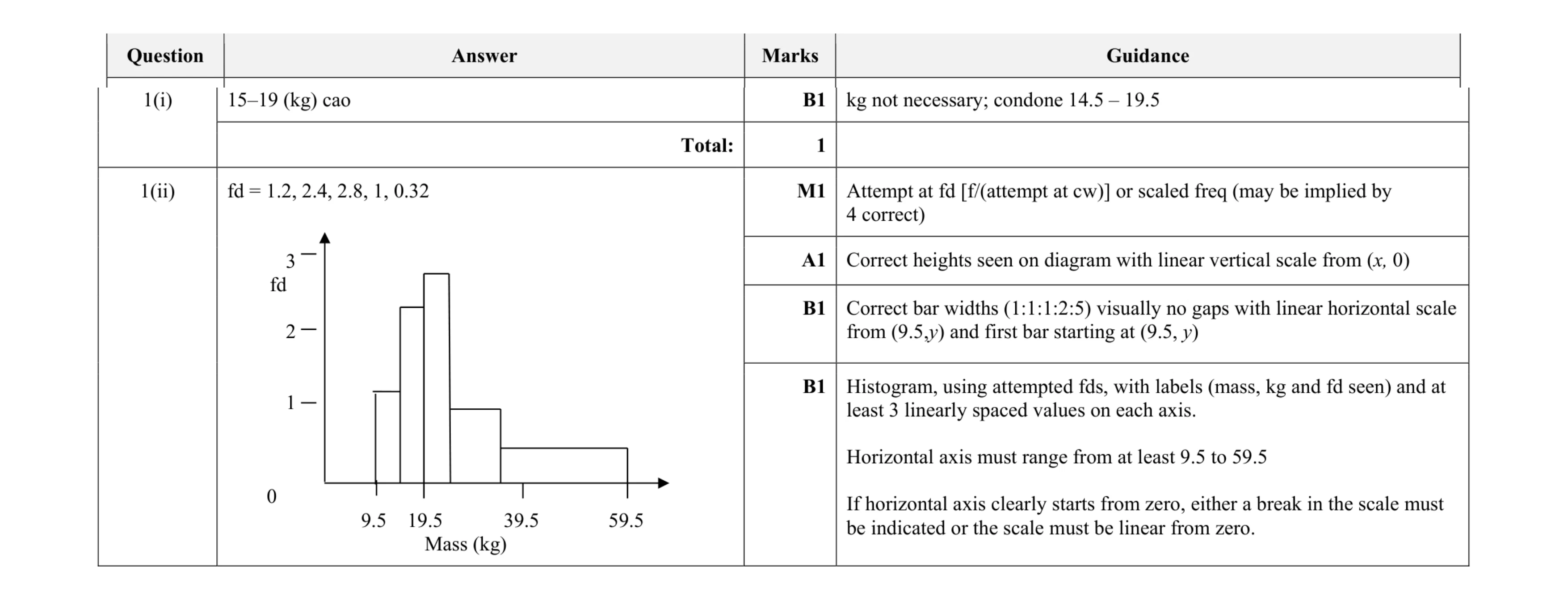 5
5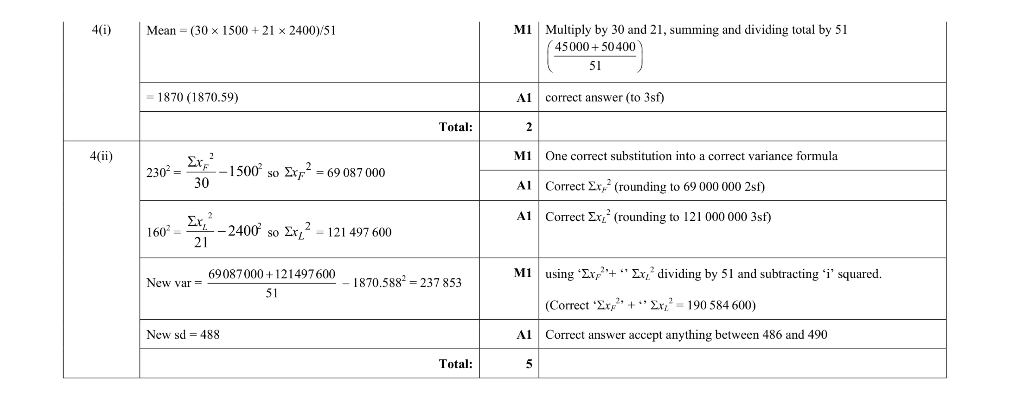 7
7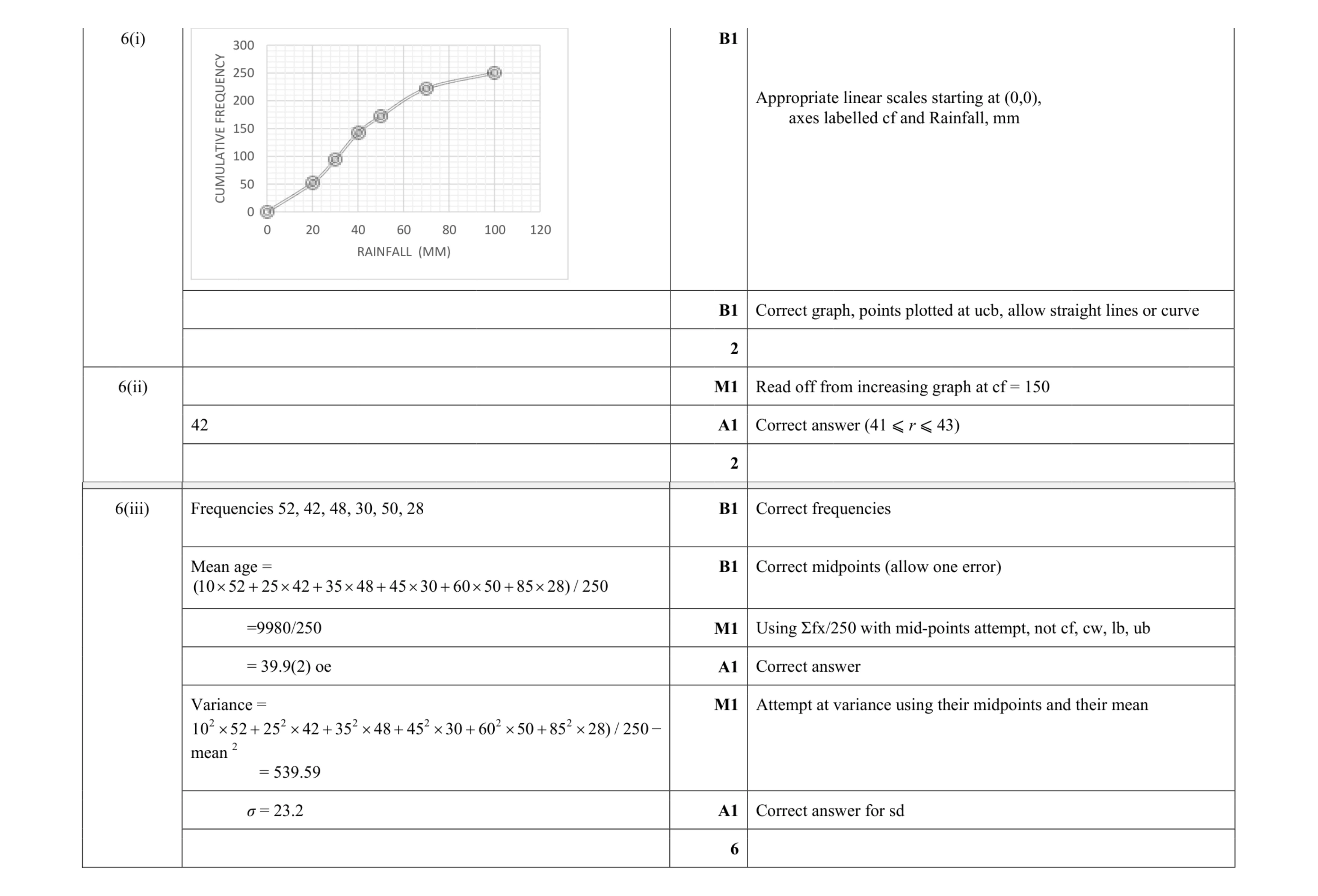 10
10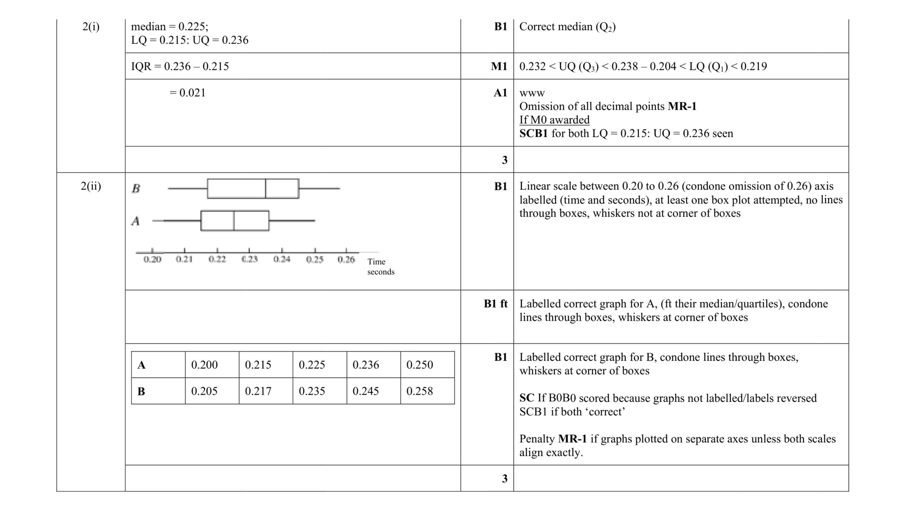 6
6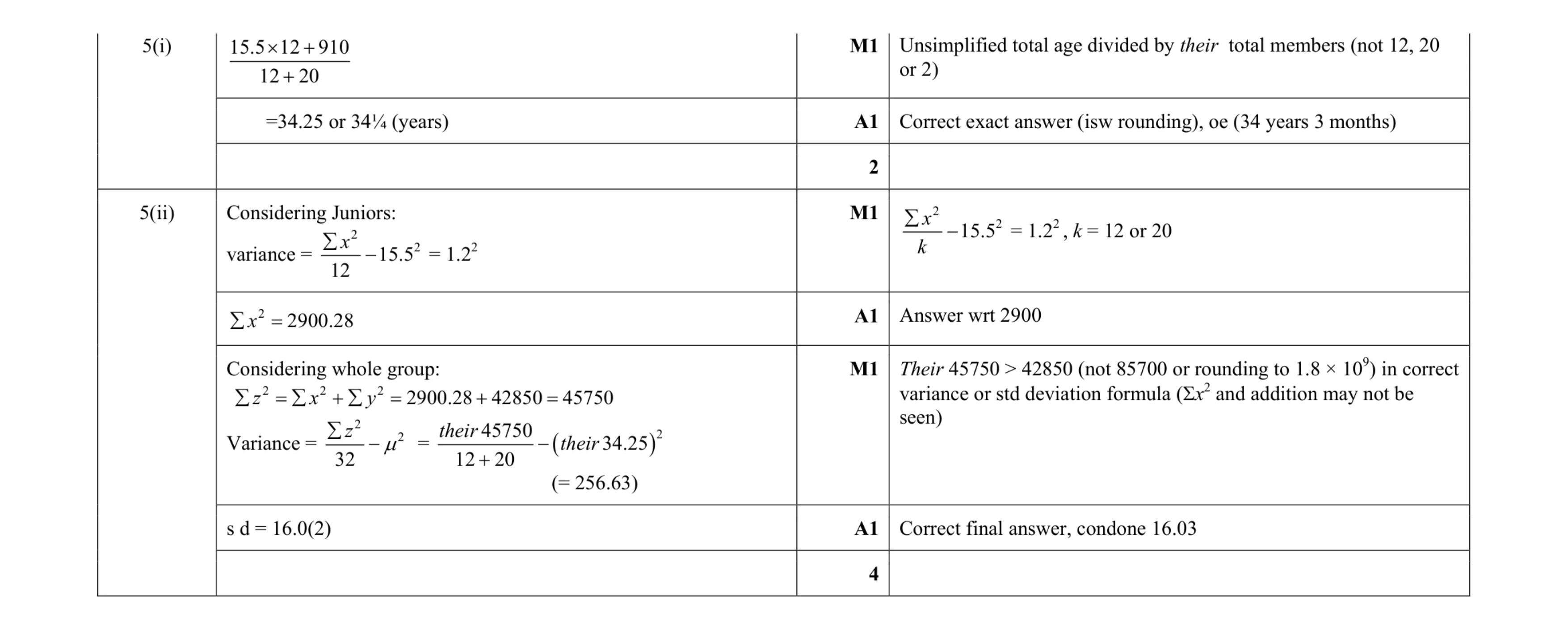 6
6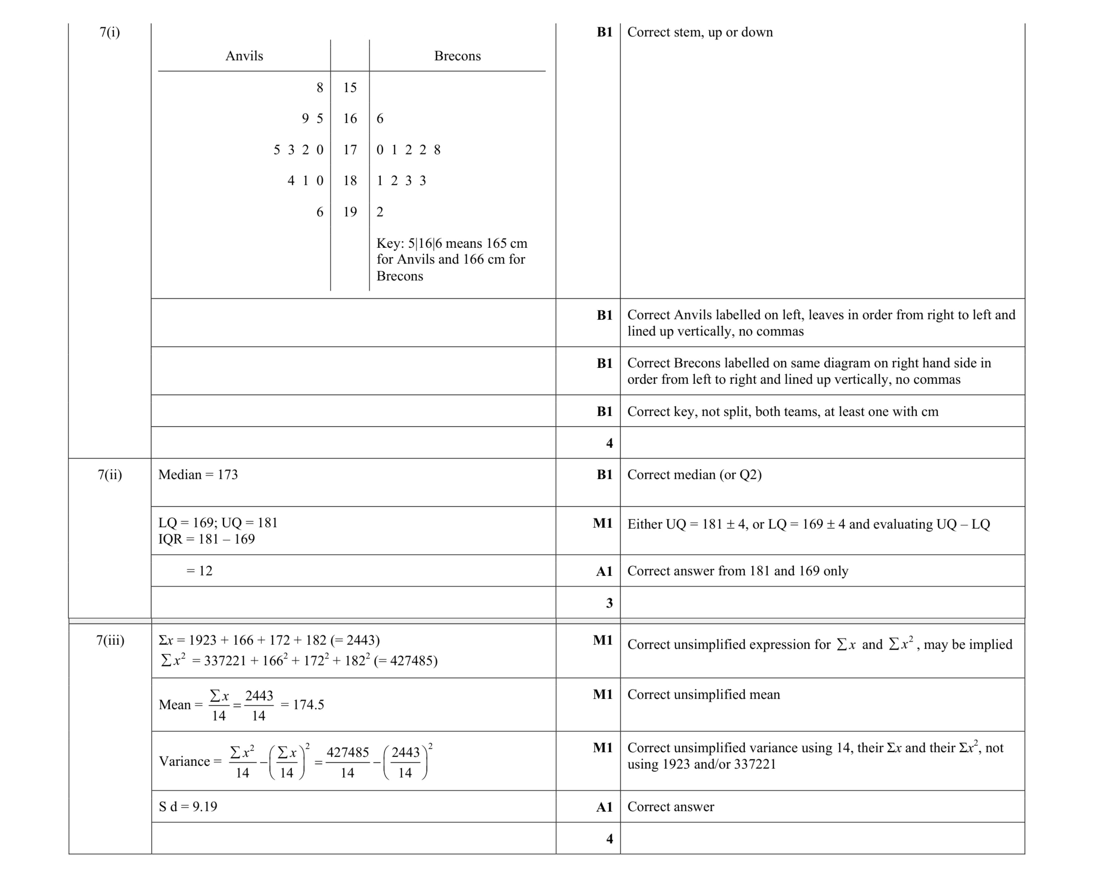 11
11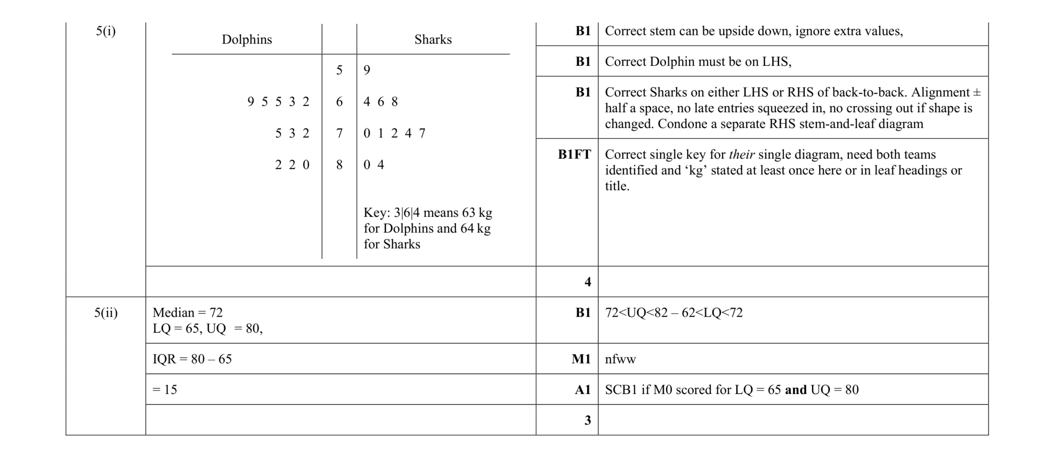 7
7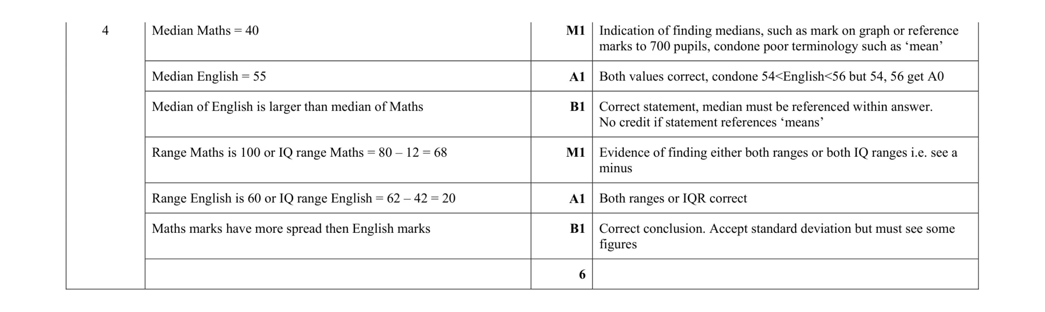 6
6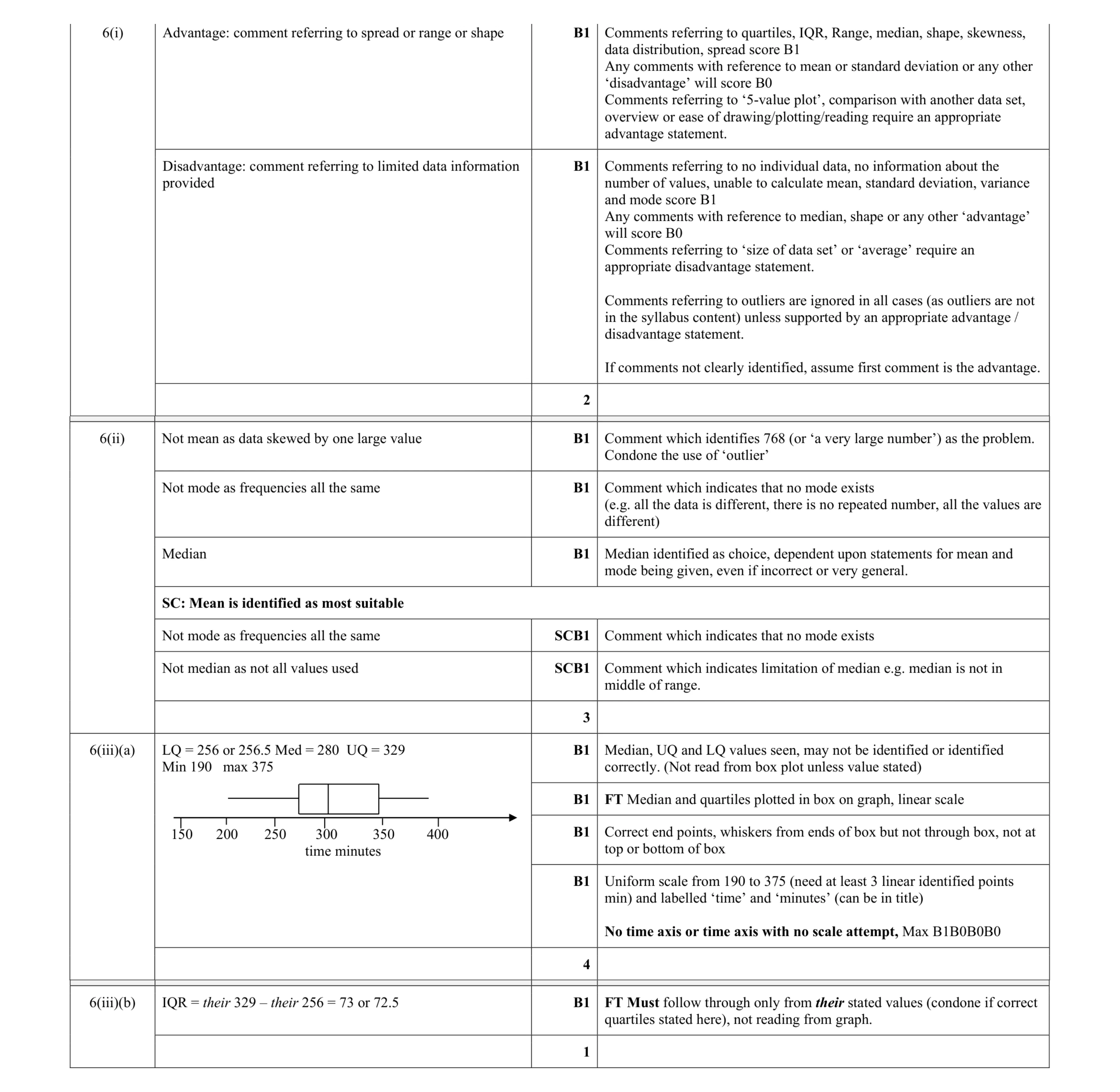 10
10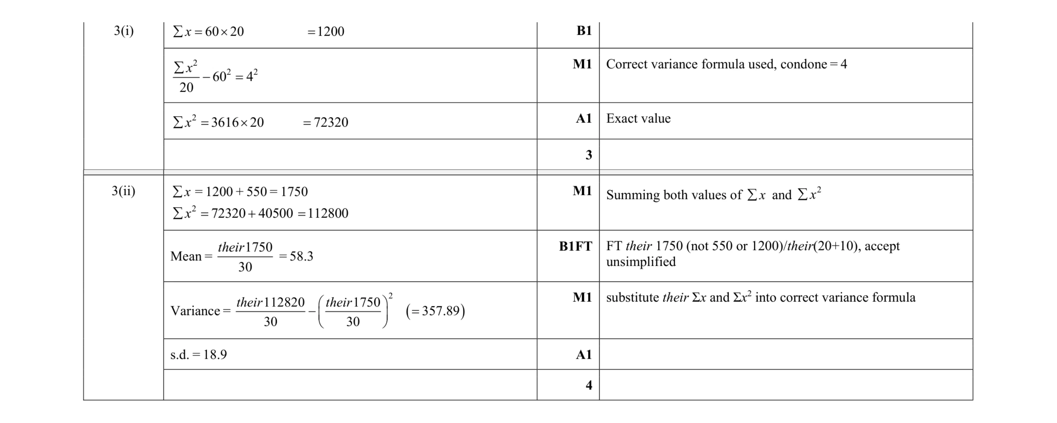 7
7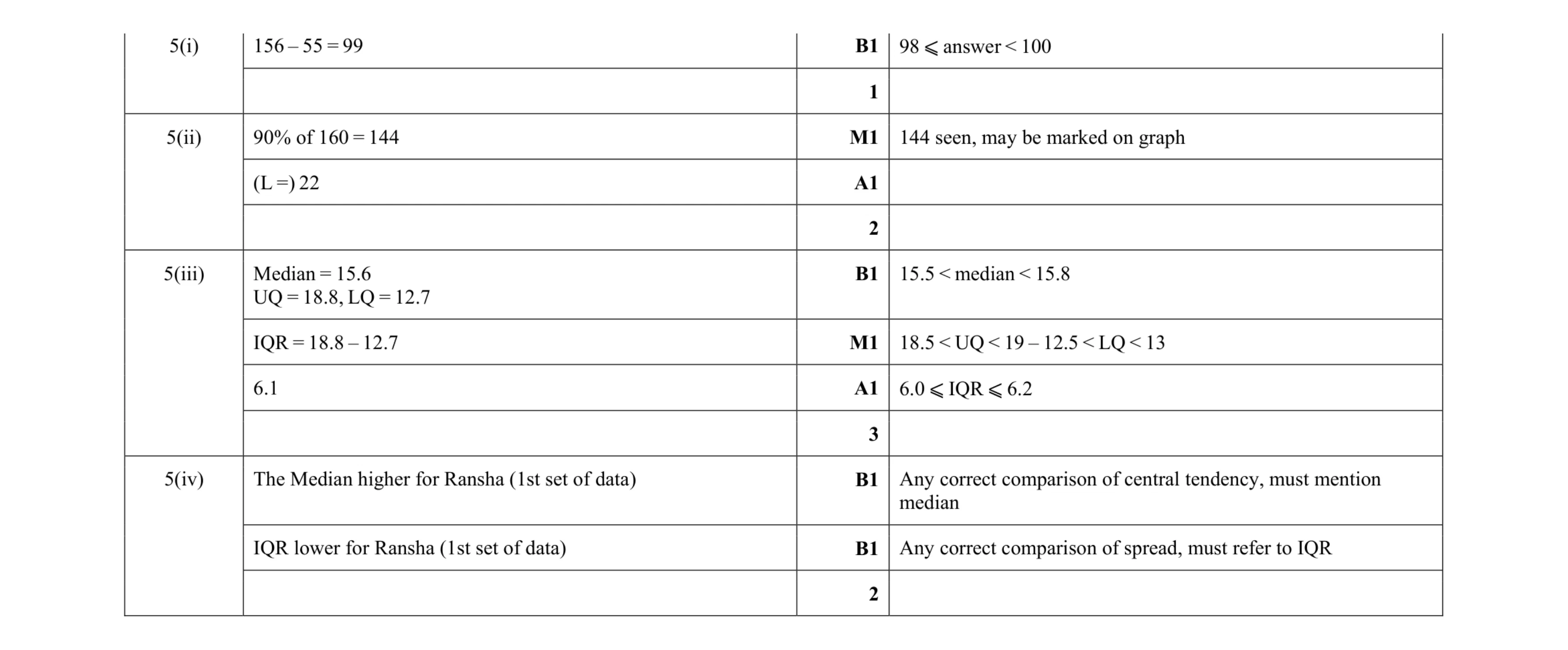 8
8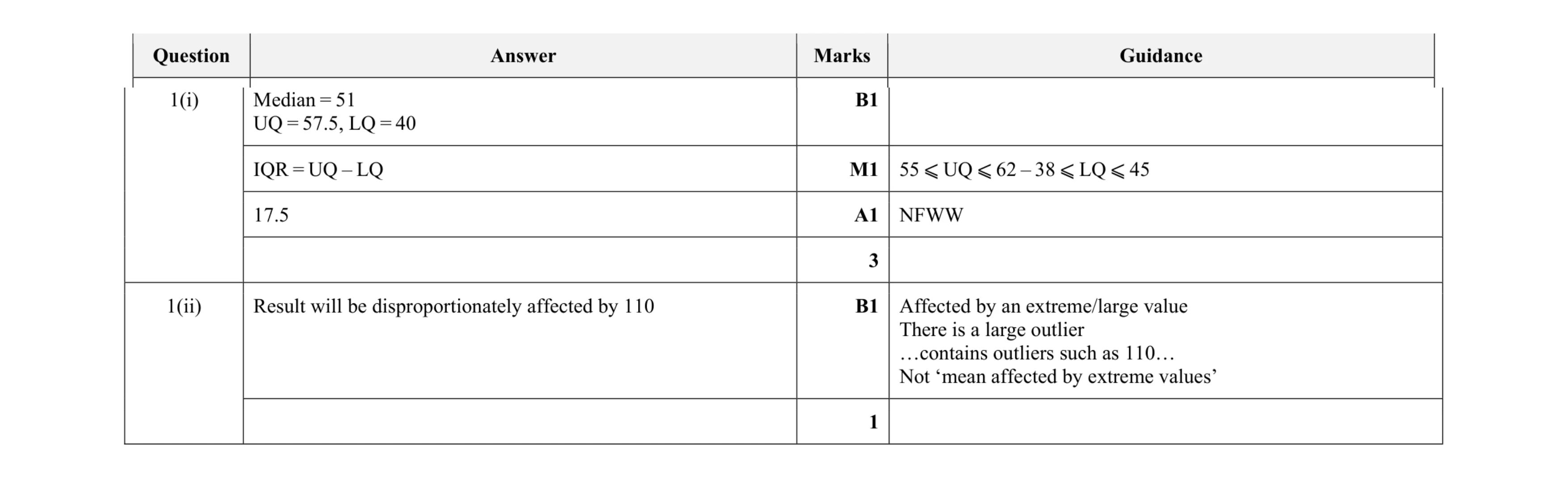 4
4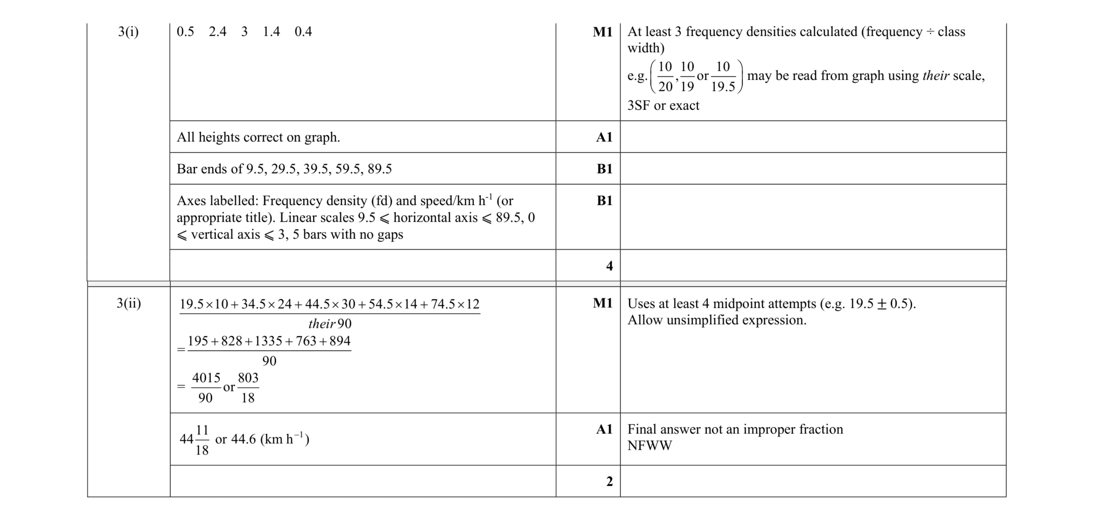 6
6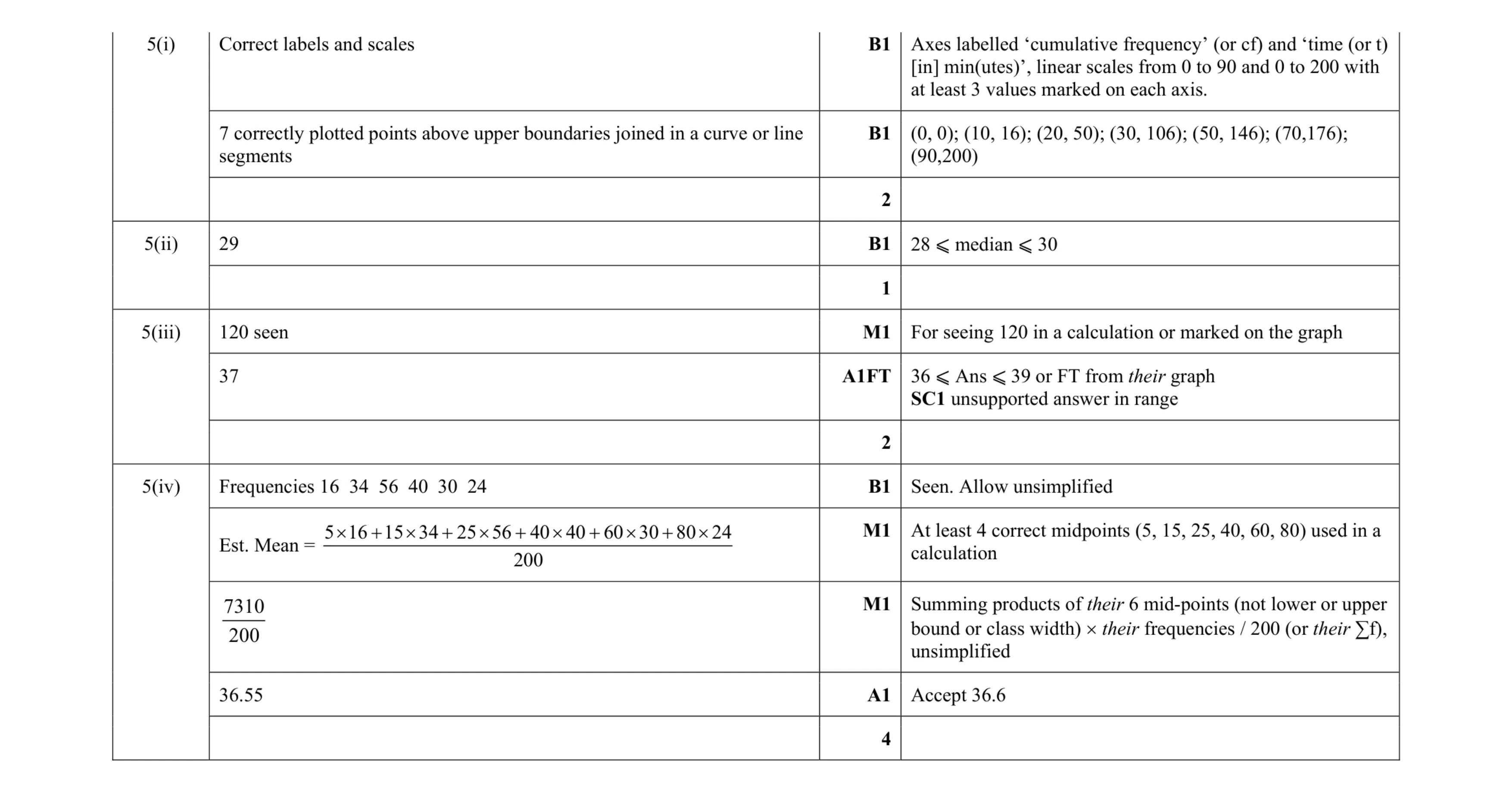 9
9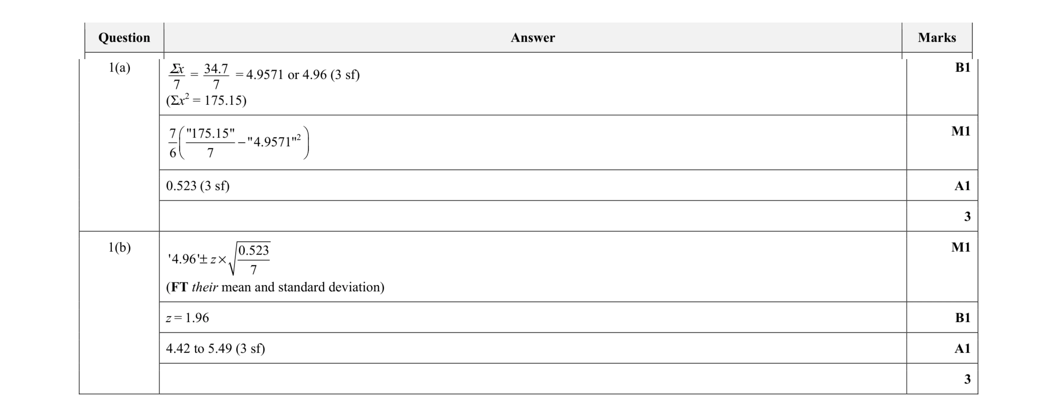 6
6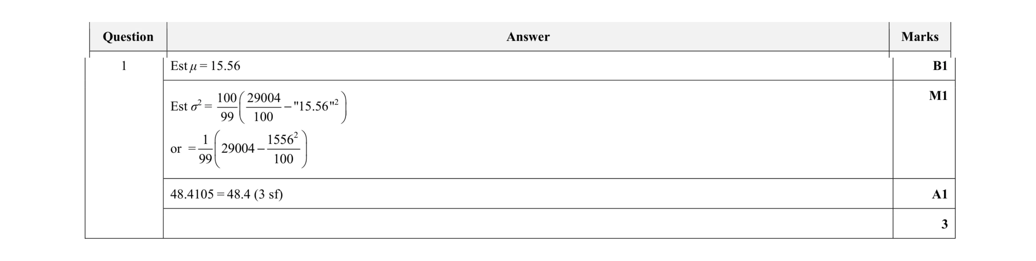 3
3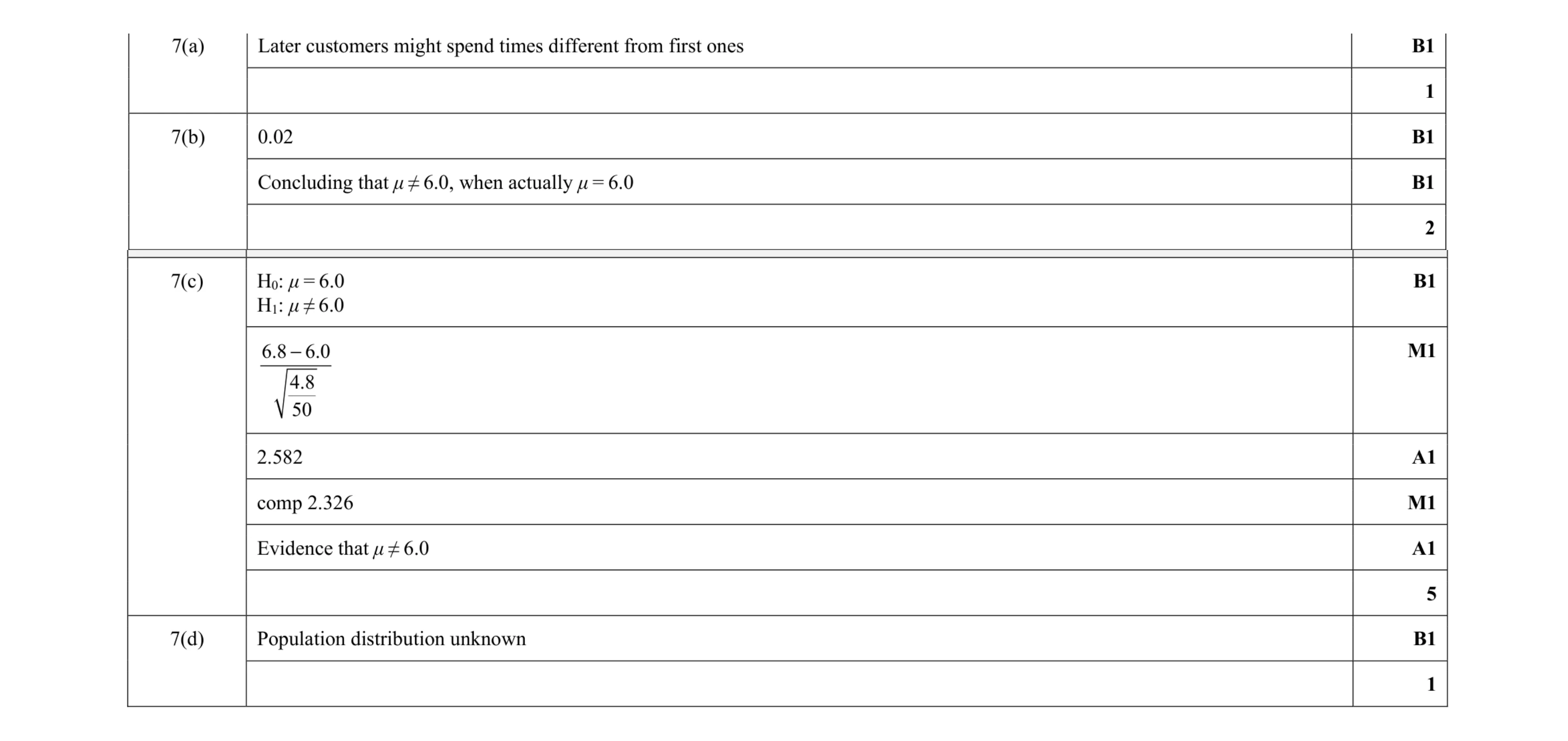 9
9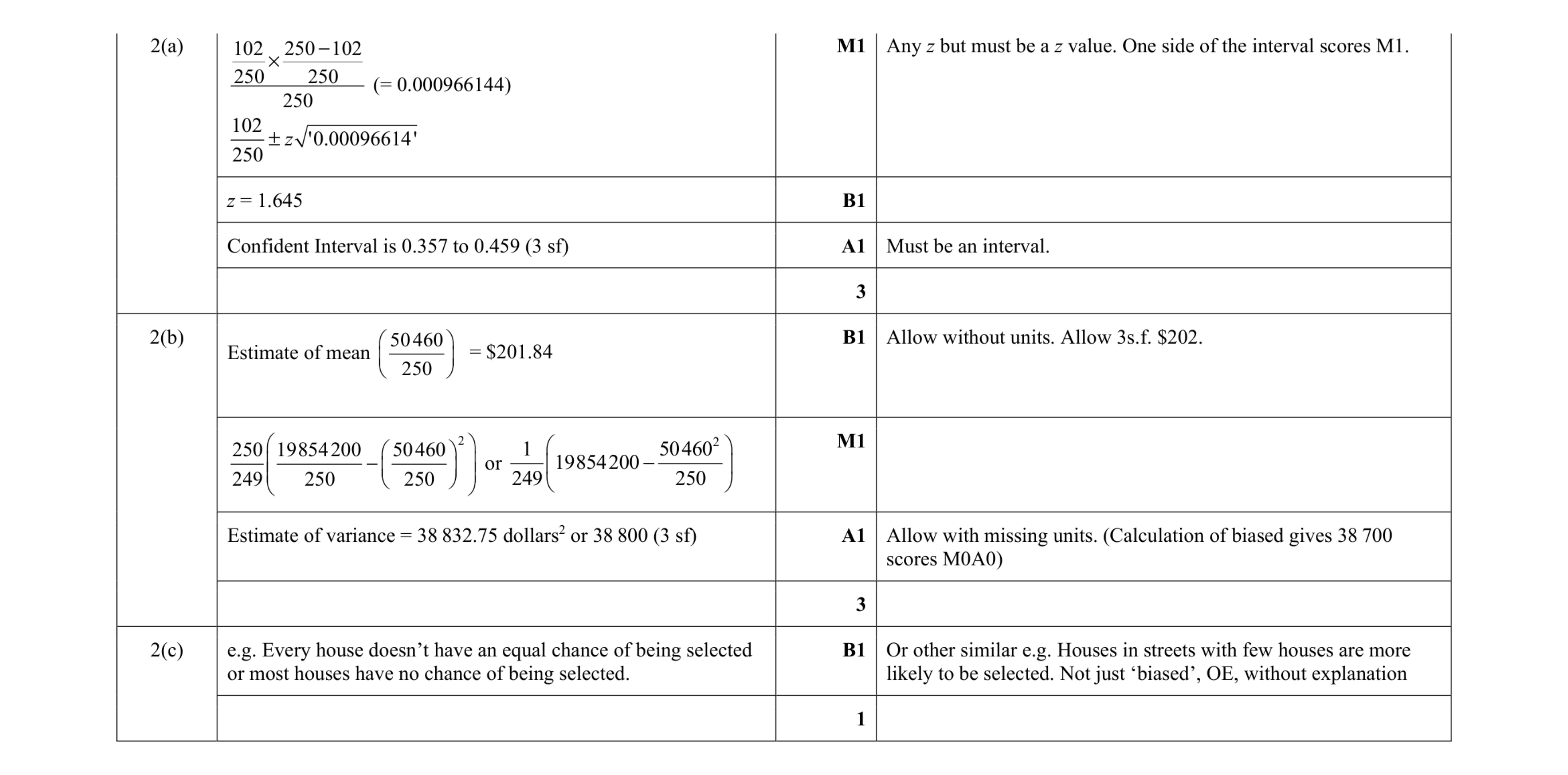 7
7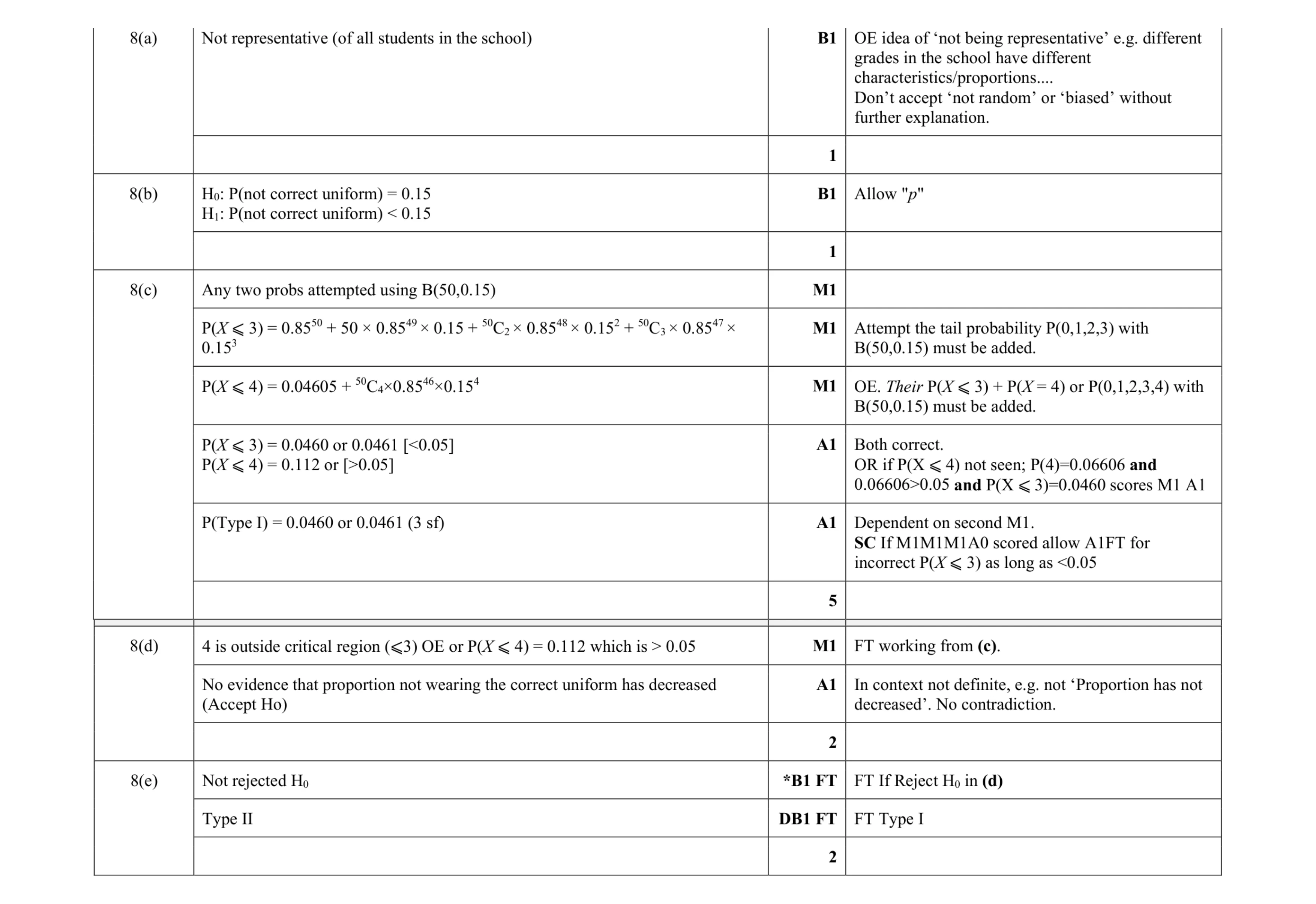 11
11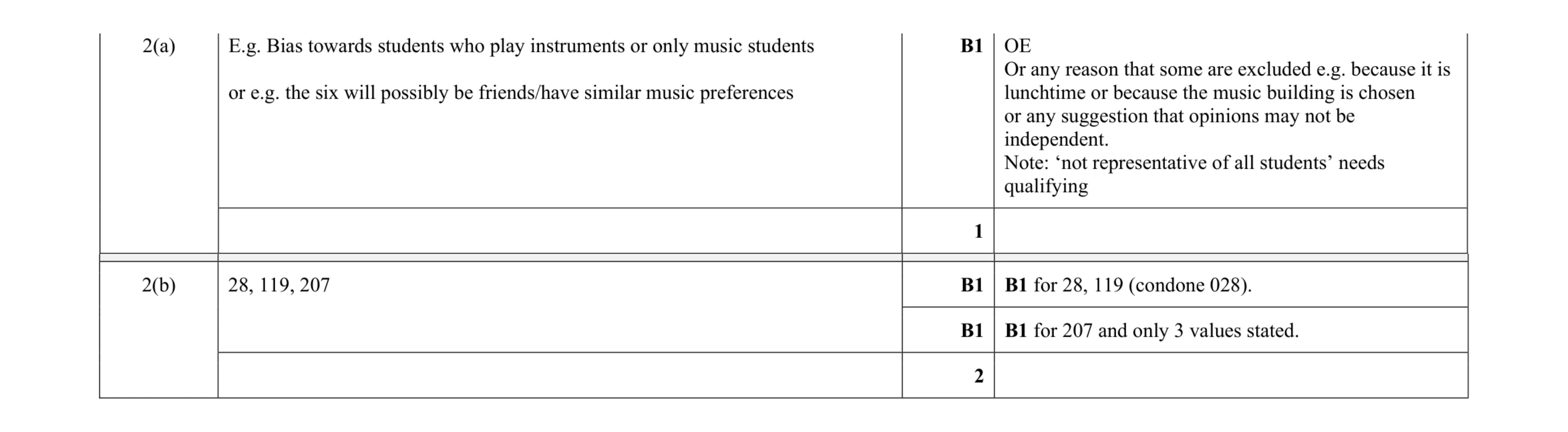 3
3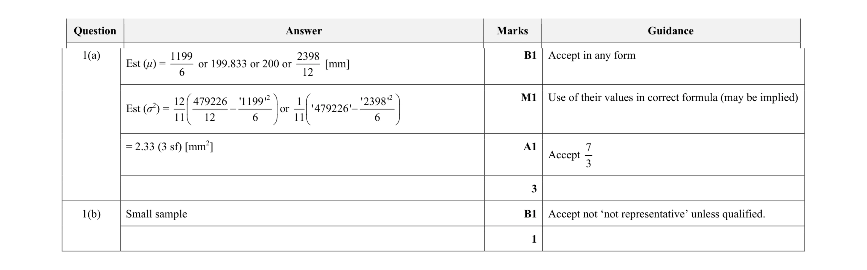 4
4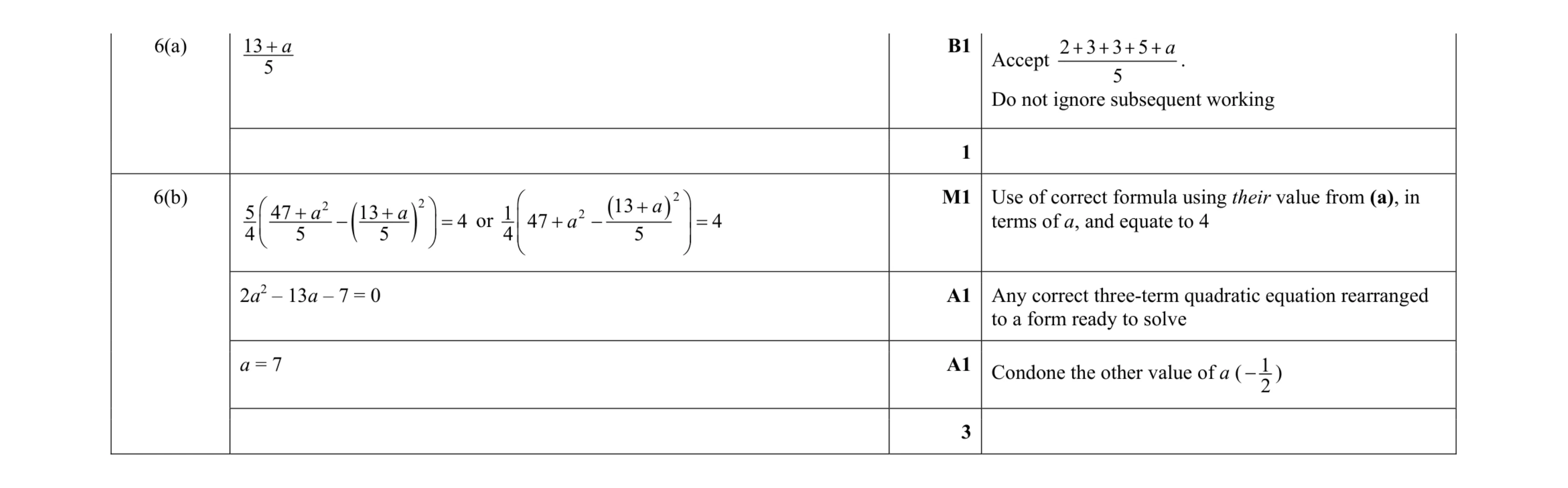 4
4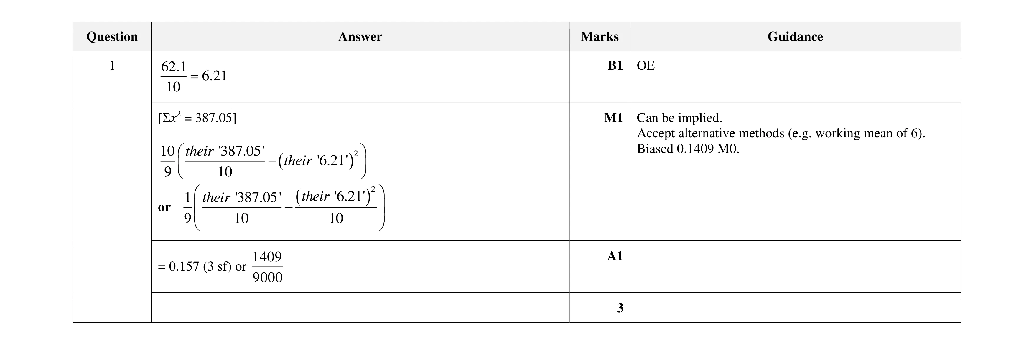 3
3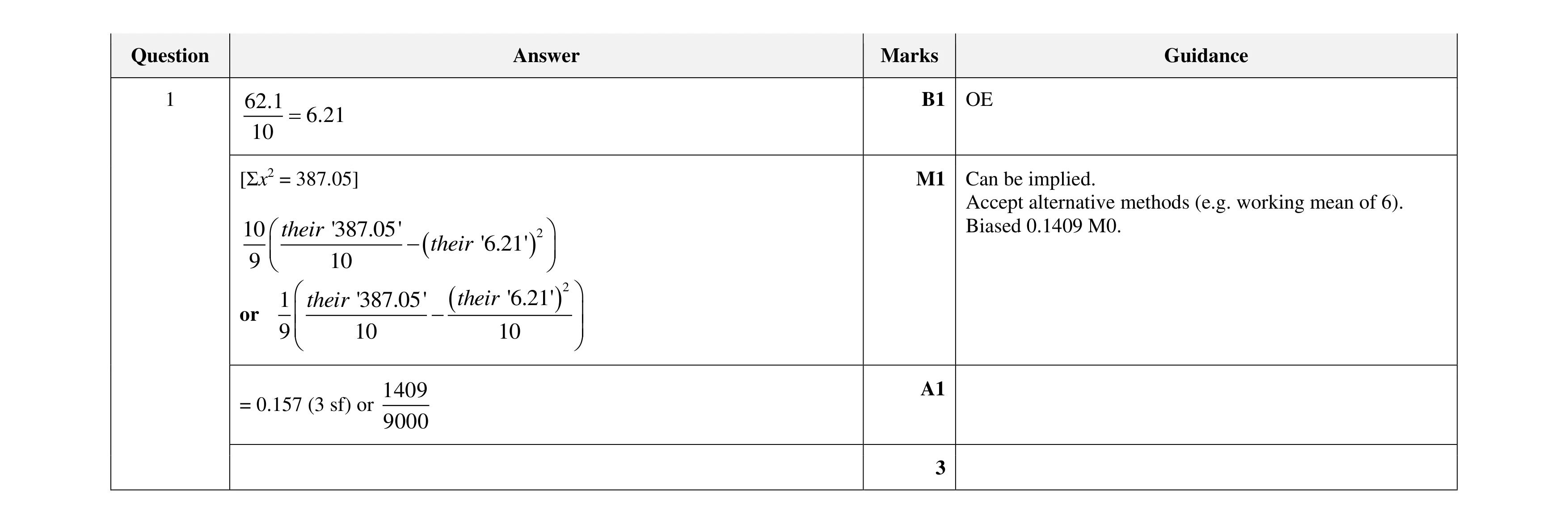 3
3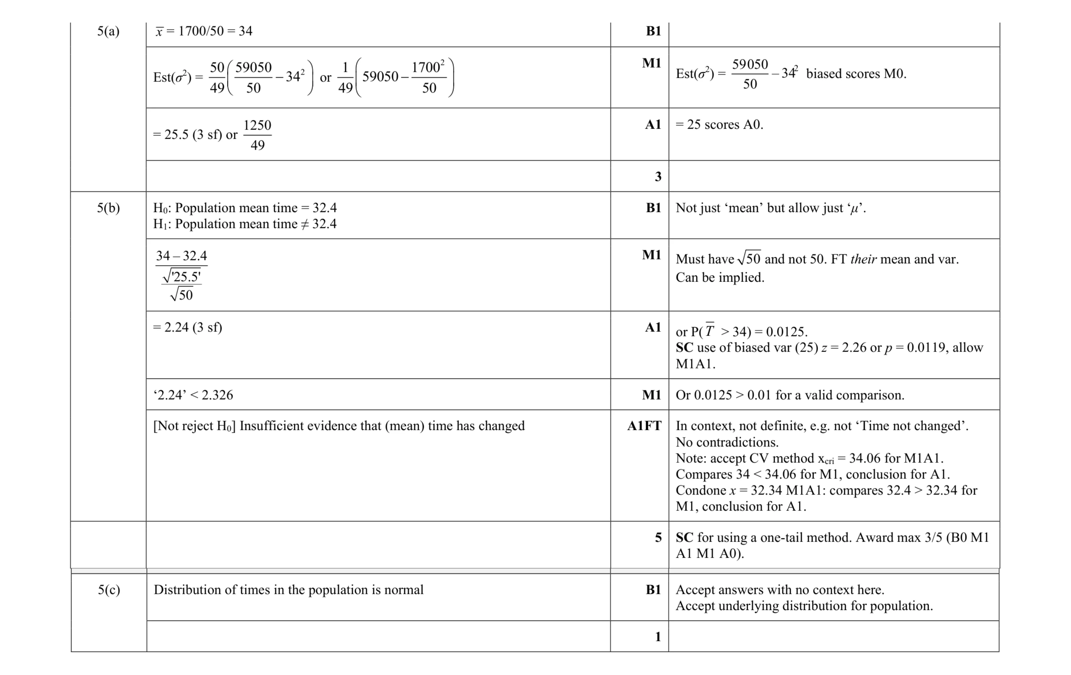 9
9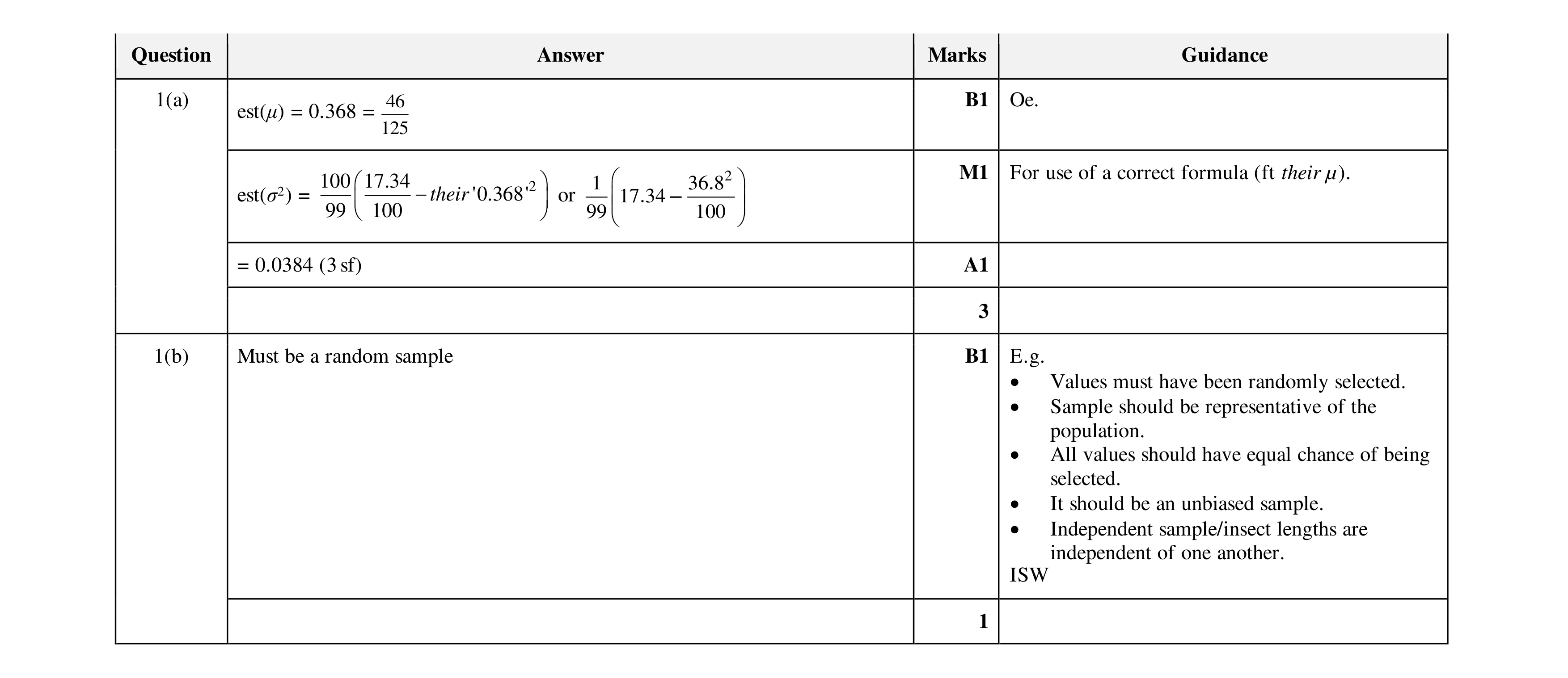 4
4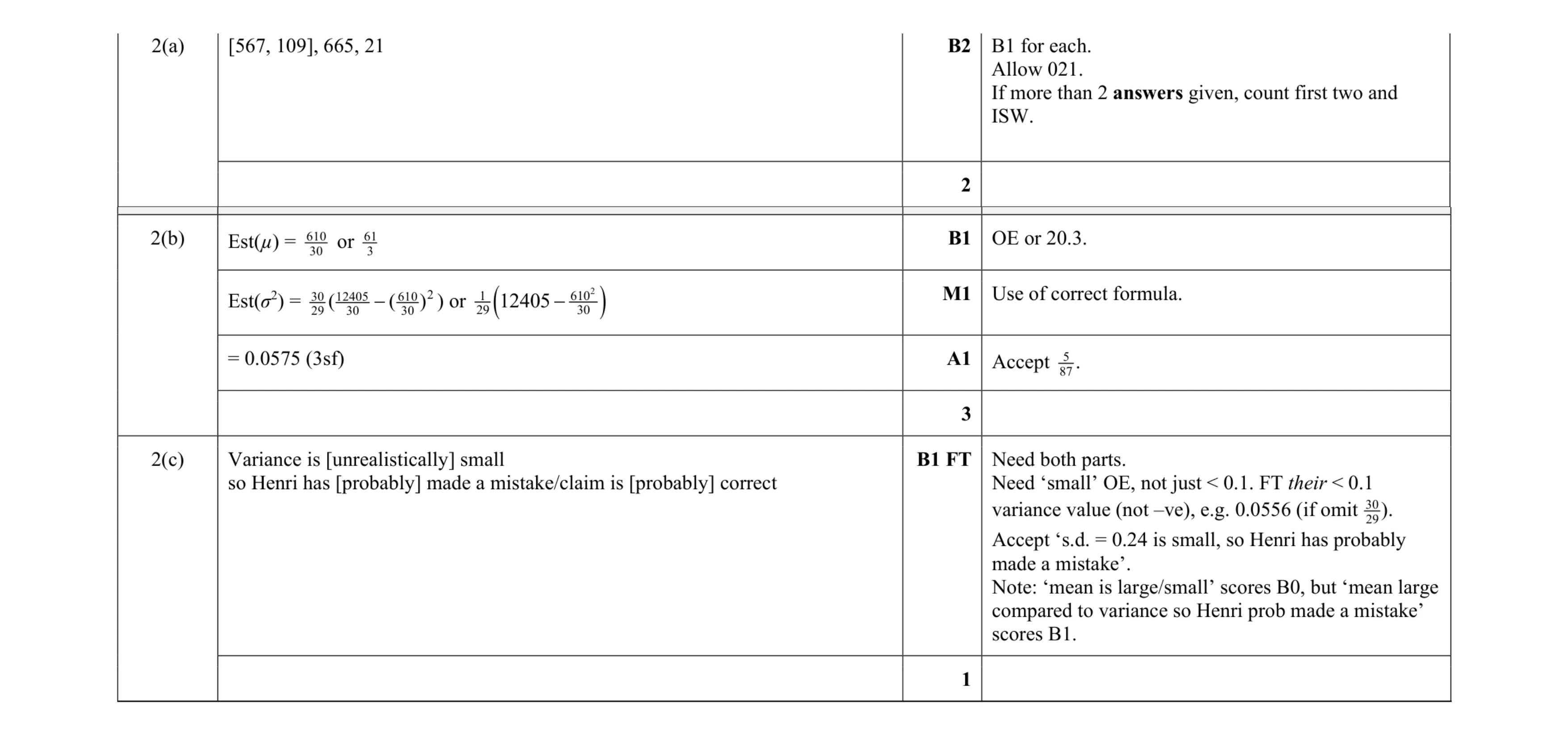 6
6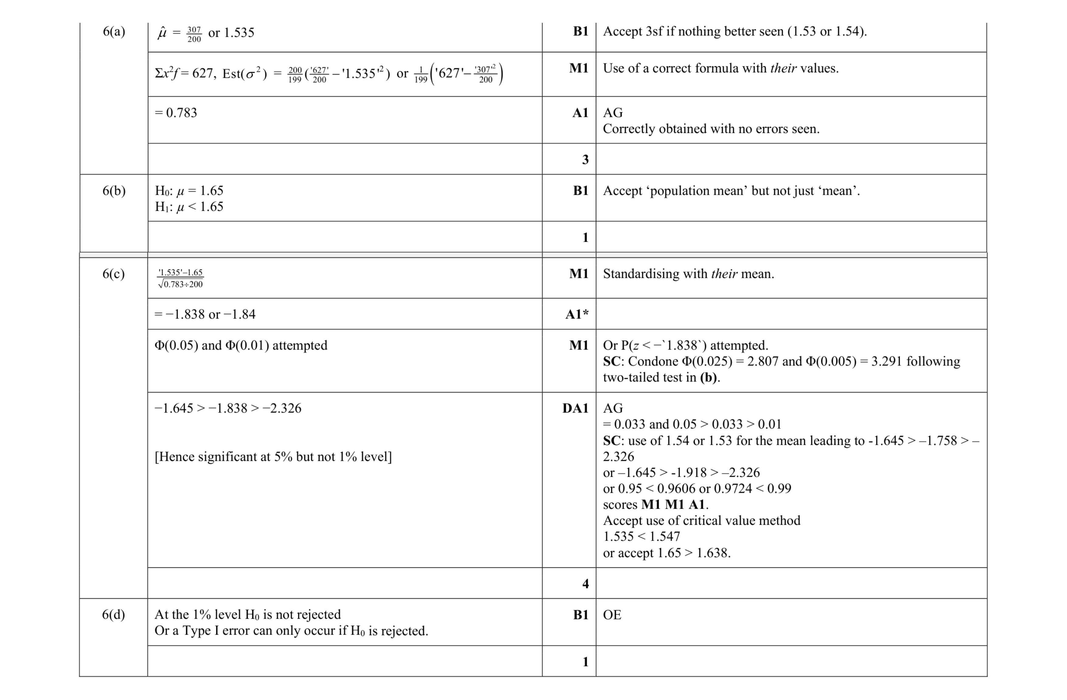 9
9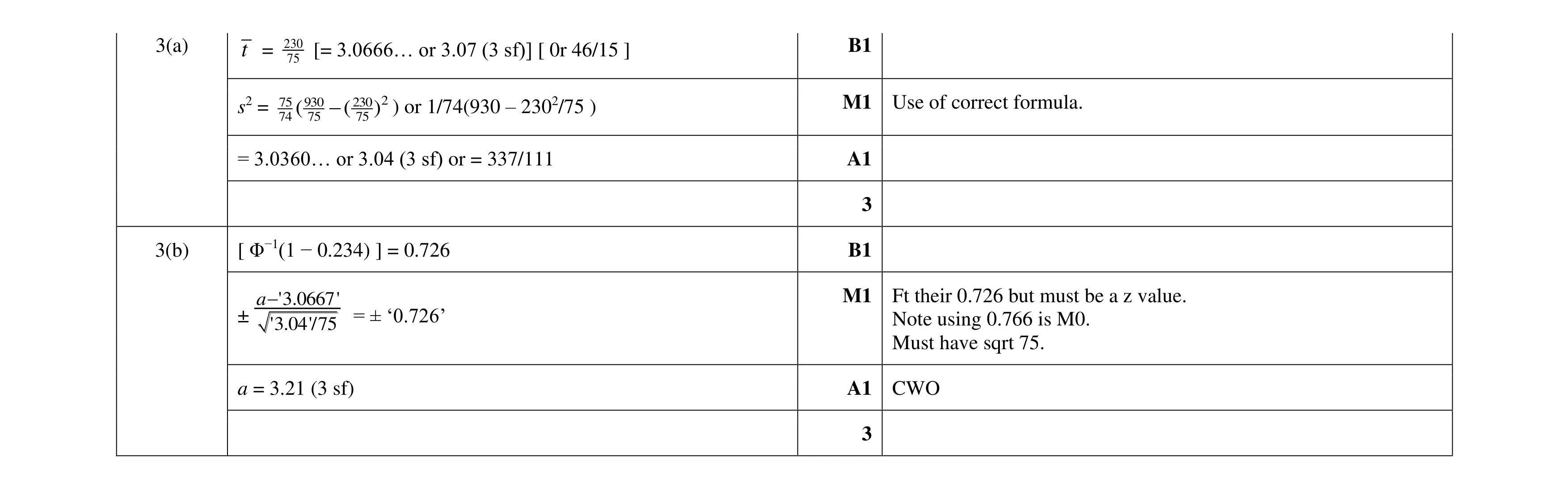 6
6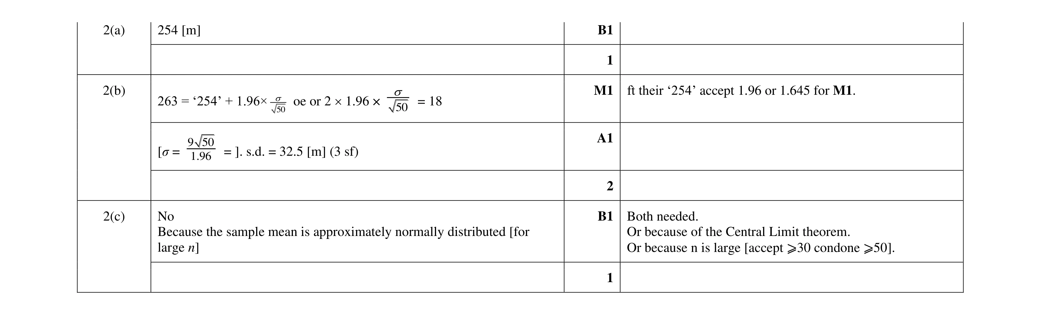 4
4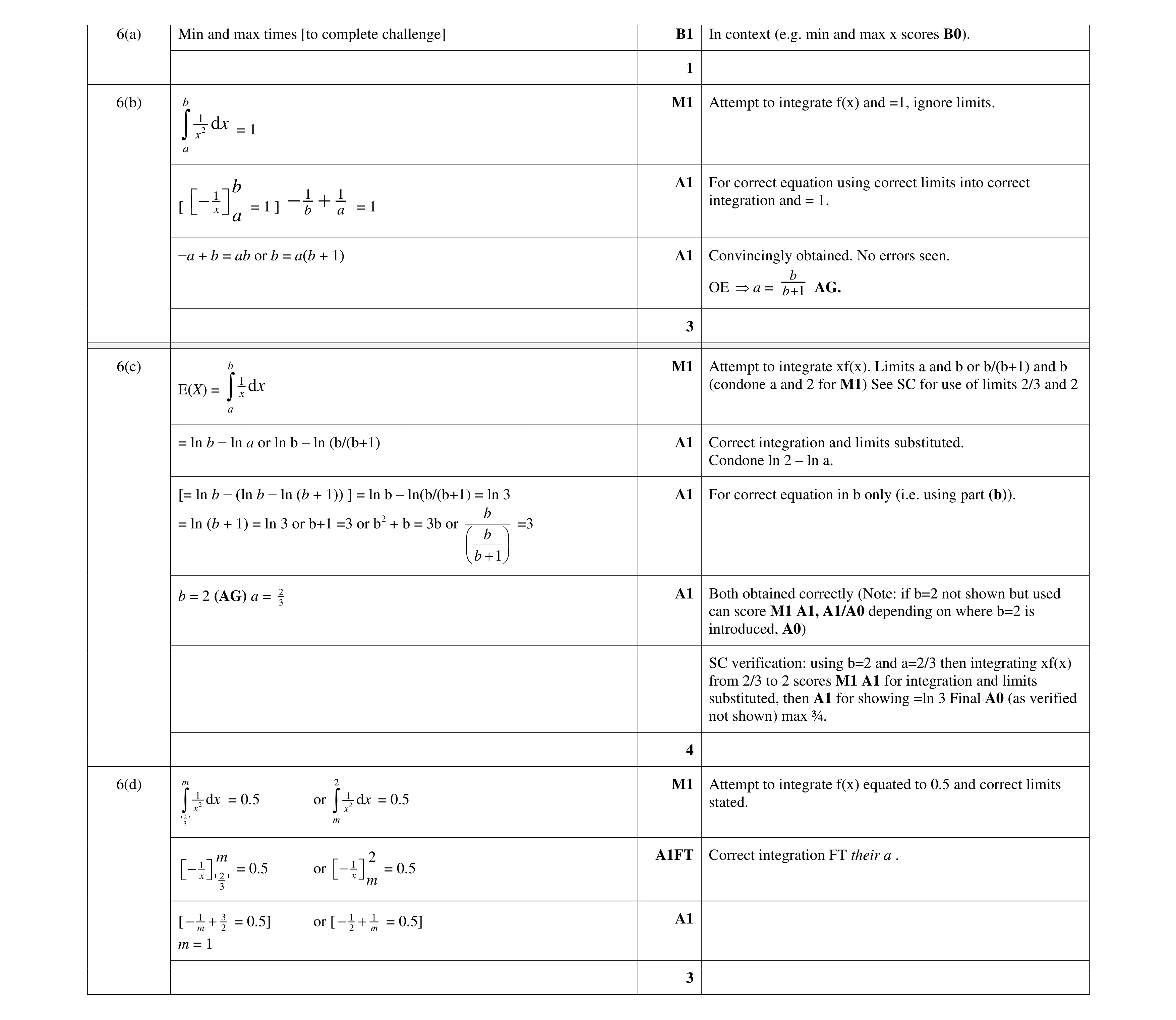 11
11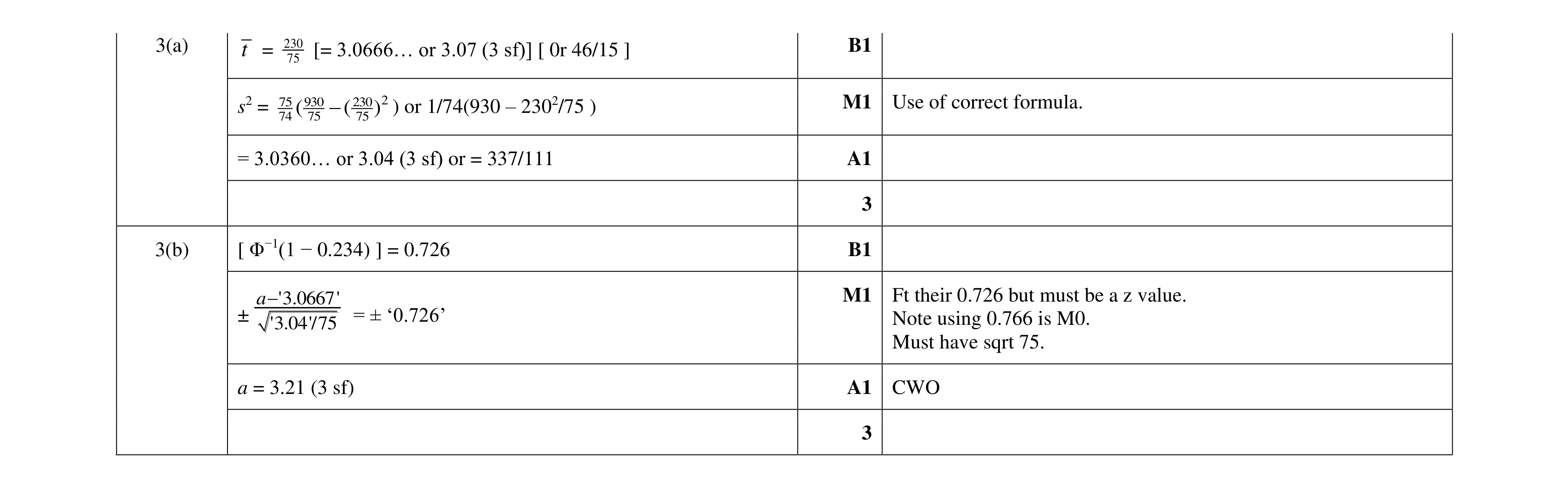 6
6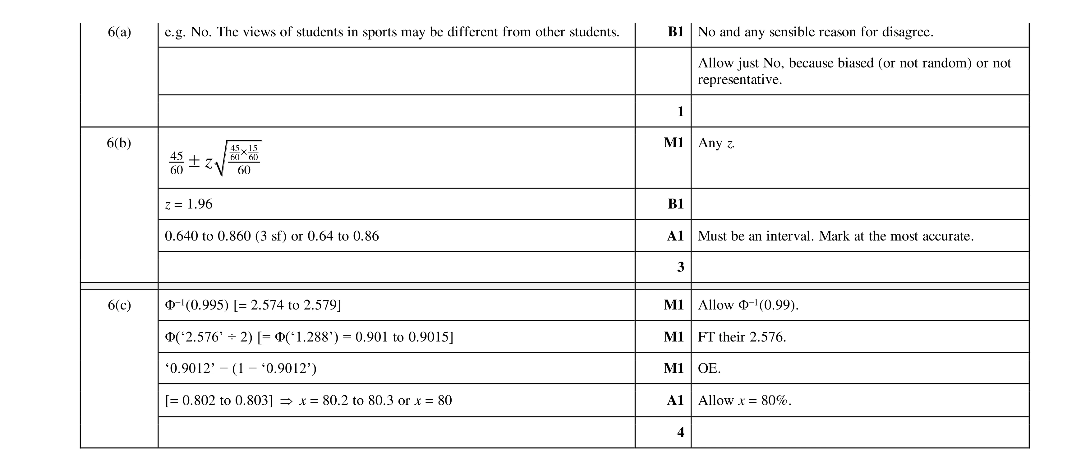 8
8 3
3