Questions as text
Q1 · Helen measures the lengths of 150 fish of a certain species in a large pond 9709/52 Feb/March 2020
7 Helen measures the lengths of 150 fish of a certain species in a large pond. These lengths, correct to the nearest centimetre, are summarised in the following table. Length (cm) 0 −9 10 −14 15 −19 20 −30 Frequency 15 48 66 21 (a) Draw a cumulative frequency graph to illustrate the data. [4] (b) 40% of these fish have a length of d cm or more. Use your graph to estimate the value of d. [2] … … … … The mean length of these 150 fish is 15.295 cm. (c) Calculate an estimate for the variance of the lengths of the fish. [3] … … … … … … … … … … … … … … … … … … …
9 marks
Mark scheme: 7(a) 15, 63, 129, 150 B1 Correct cumulative frequencies seen (may be on graph) B1 0 ⩽ Horizontal axis ⩽ 30, 0 ⩽ vertical axis ⩽ 150 Labels correct: length cm, cf M1 At least 3 points plotted at upper end points (e.g. allow 9, 9.5, 10) with a linear horizontal scale. A1 Linear vertical scale, all points at correct upper end points (9.5 etc.), curve drawn accurately, joined to (0,0) (condone (–0.5, 0)) 4 7(b) 60% of 150 = 90 M1 90 seen or implied by use on graph Approx. 16.5 [cm] A1FT FT their increasing cumulative frequency graph, Use of graph must be seen. If no clear evidence of use of graph SCB1FT correct value from their graph 2 7(c) Midpoints: 4.75, 12, 17, 25 M1 At least 3 correct midpoints used (39449.4375 implies M1) 4.75 2 × 15 + 12 2 × 48 + 17 2 × 66 + 25 2 × 21 2 M1 Using midpoints ±0.5 in correct var formula, including Var = − 15.295 subtraction of their µ2. 150 = 29.1 A1 3
This question in 9709/52 Feb/March 2020
Q2 · The numbers of chocolate bars sold per day in a cinema over a period of 100 days are… 9709/51 May/June 2020
7 The numbers of chocolate bars sold per day in a cinema over a period of 100 days are summarised in the following table. Number of chocolate bars sold 1 −10 11 −15 16 −30 31 −50 51 −60 Number of days 18 24 30 20 8 (a) Draw a histogram to represent this information. [5] (b) What is the greatest possible value of the interquartile range for the data? [2] … … … … … … … (c) Calculate estimates of the mean and standard deviation of the number of chocolate bars sold. [4] … … … … … … … … … … … … … … … …
11 marks
Mark scheme: 7(a) Class widths: 10, 5, 15, 20, 10 M1 Frequency density = frequency/their class width: 1.8, 4.8, 2, 1, 0.8 M1 All heights correct on diagram (using a linear scale) A1 Correct bar ends B1 Bar ends: 10.5, 15.5, 30.5, 50.5, 60.5 B1 5 7(b) 11 – 15 and 31 – 50 B1 Greatest IQR = 50 – 11 = 39 B1 2 7(c) Mean = 18 5.5 24 13 30 23 20 40.5 8 55.5 2355 23.6 100 100 × + × + × + × + × = = B1 Var = 2 2 2 2 2 2 18 5.5 24 13 30 23 20 40.5 8 55.5 mean 100 × + × + × + × + × − M1 2 77917.5 mean 224.57 100 − = A1 Standard deviation = 15.0 (FT their variance) A1 FT 4
This question in 9709/51 May/June 2020
Q3 · Two machines, A and B, produce metal rods of a certain type 9709/52 May/June 2020
3 Two machines, A and B, produce metal rods of a certain type. The lengths, in metres, of 19 rods produced by machine A and 19 rods produced by machine B are shown in the following back-to-back stem-and-leaf diagram. A B 21 1 2 4 7 6 3 0 22 2 4 5 5 6 8 7 4 3 1 1 23 0 2 6 8 9 9 5 5 5 3 2 24 3 3 4 6 4 3 1 0 25 6 Key: 7 22 4 means 0.227 m for machine A and 0.224 m for machine B. (a) Find the median and the interquartile range for machine A. [3] … … … … … … … … … … … … … … … … … … It is given that for machine B the median is 0.232 m, the lower quartile is 0.224 m and the upper quartile is 0.243 m. (b) Draw box-and-whisker plots for A and B. [3] (c) Hence make two comparisons between the lengths of the rods produced by machine A and those produced by machine B. [2] … … … … … … … … … …
8 marks
Mark scheme: 3(a) B1 UQ = 0.245, LQ = 0.231, So IQR = 0.245 – 0.231 M1 0.014 A1 3 Question Answer Marks 3(b) LQ M UQ A 0.220 0.231 FT 0.238 FT 0.245 FT 0.254 B 0.211 0.224 0.232 0.243 0.256 Medians and quartiles correctly plotted for A or B B1 End points correct for A or B B1 Completely correct, including scale B1 3 3(c) Lengths of rods produced by machine A are longer. (B1 for comparison of central tendency) B1 Lengths of rods produced by machine A are less spread out (B1 for comparison of spread) B1 2
This question in 9709/52 May/June 2020
Q4 · The annual salaries, in thousands of dollars, for 11 employees at each of two companies A… 9709/53 May/June 2020
6 The annual salaries, in thousands of dollars, for 11 employees at each of two companies A and B are shown below. Company A 30 32 35 41 41 42 47 49 52 53 64 Company B 26 47 30 52 41 38 35 42 49 31 42 (a) Represent the data by drawing a back-to-back stem-and-leaf diagram with company A on the left-hand side of the diagram. [4] (b) Find the median and the interquartile range of the salaries of the employees in company A. [3] … … … … … … … … … A new employee joins company B. The mean salary of the 12 employees is now $38 500. (c) Find the salary of the new employee. [3] … … … … … … … … … … … … … …
10 marks
Mark scheme: 6(a) A B 2 6 5 2 0 3 0 1 5 8 9 7 2 1 1 4 1 2 2 7 9 3 2 5 2 4 6 KEY 1 | 4 | 2 means $41 000 for A and $42 000 for B Correct stem B1 Correct A on LHS B1 Correct B on same diagram B1 Correct key for their diagram, both companies identified and correct units B1 4 6(b) Median = [$]42 000 B1 LQ = [$]35 000 UQ = [$]52 000 B1 IQR = [$]17 000 (FT if 49000 UQ 53000 32000 LQ 41000 − ≤ ≤ ≤ ≤ ) B1 FT 3 Question Answer Marks 6(c) Sum of given 11 numbers is 433 000 M1 Sum of 12 numbers, including new = 38 500 × 12 = 462 000 M1 Difference = new salary = [$]29 000 A1 3
This question in 9709/53 May/June 2020
Q5 · The times, t minutes, taken by 150 students to complete a particular challenge are… 9709/51 Oct/Nov 2020
6 The times, t minutes, taken by 150 students to complete a particular challenge are summarised in the following cumulative frequency table. Time taken (t minutes) t ≤20 t ≤30 t ≤40 t ≤60 t ≤100 Cumulative frequency 12 48 106 134 150 (a) Draw a cumulative frequency graph to illustrate the data. [2] (b) 24% of the students take k minutes or longer to complete the challenge. Use your graph to estimate the value of k. [2] … … … … … (c) Calculate estimates of the mean and the standard deviation of the time taken to complete the challenge. [6] … … … … … … … … … … … … … … … … … …
10 marks
Mark scheme: 6(a) M1 At least 4 points plotted at upper end points, with both scales linear with at least 3 values indicated Correct cumulative frequency curve A1 All plotted correctly with curve drawn joined to (0, 0), axes labelled cumulative frequency, time, minutes 2 6(b) 150 × 0·76 = 114 M1 114 SOI, may be on graph k = 45 (mins) A1 FT Clear indication that their graph has been used, tolerance ±1mm 2 Question Answer Marks Guidance 6(c) Frequencies: 12 36 58 28 16 B1 Correct frequencies seen Mean = 10 12 25 36 35 58 50 28 80 16 150 × + × + × + × + × B1 At least 4 correct midpoints seen and used 120 900 2030 1400 1280 150 + + + + M1 Correct formula with their midpoints (not upper boundary, lower boundary, class width or frequency density). 38.2, 38 1 5 A1 Variance = 2 2 2 2 2 2 12 10 36 25 58 35 28 50 16 80 150 mean × + × + × + × + × − = 2 1200 22500 71050 70000 102400 150 mean + + + + − M1 Substitute their midpoints and frequencies (condone use of cumulative frequency) in correct variance formula, must have ‘– their mean2’ (Standard deviation = 321.76 ) = 17.9 A1 6
This question in 9709/51 Oct/Nov 2020
Q6 · The following table gives the weekly snowfall, in centimetres, for 11 weeks in 2018 at… 9709/52 Oct/Nov 2020
5 The following table gives the weekly snowfall, in centimetres, for 11 weeks in 2018 at two ski resorts, Dados and Linva. Dados 6 8 12 15 10 36 42 28 10 22 16 Linva 2 11 15 16 0 32 36 40 10 12 9 (a) Represent the information in a back-to-back stem-and-leaf diagram. [4] (b) Find the median and the interquartile range for the weekly snowfall in Dados. [3] … … … … … … … … … (c) The median, lower quartile and upper quartile of the weekly snowfall for Linva are 12, 9 and 32 cm respectively. Use this information and your answers to part (b) to compare the central tendency and the spread of the weekly snowfall in Dados and Linva. [2] … … … … … … … … … … … … … …
9 marks
Mark scheme: 5(a) Dados Linva 8 6 0 0 2 9 6 5 2 0 0 1 0 1 2 5 6 8 2 2 6 3 2 6 2 4 0 KEY 6| 3| 2 means 36 cm (snow) in Dados and 32 cm (snow) in Linva B1 Correct stem can be upside down, ignore extra values B1 Correct Dados labelled, leaves in order and lined up vertically (less than midway to next column), no commas etc, no extra terms B1 Correct Linva on opposite side of stem labelled, leaves in order and lined up vertically (less than midway to next column), no commas etc, no extra terms B1 Correct single key for their diagram, need both resorts identified and ‘cm’ stated at least once here or in leaf headings or title. SC If 2 separate diagrams drawn, SCB1 if both keys meet these criteria B0B1B0SCB1 max. 4 5(b) Median or Q2 = 15 (cm) B1 Correct UQ or Q3 = 28 cm, LQ or Q1 = 10 cm IQR = 28 – 10 M1 22 ⩽ UQ ⩽ 36 – 8 ⩽ LQ ⩽ 10 18 (cm) A1 WWW 3 5(c) On average the snowfall in Davos is higher B1 FT FT from their 5(b) values for Dados. Statement comparing central tendency in context The amount of snowfall in Linva varies more than in Davos B1 FT Statement comparing spread in context Note: simply stating and comparing the values is not sufficient. 2
This question in 9709/52 Oct/Nov 2020
Q7 · A particular piece of music was played by 91 pianists and for each pianist, the number of… 9709/53 Oct/Nov 2020
7 A particular piece of music was played by 91 pianists and for each pianist, the number of incorrect notes was recorded. The results are summarised in the table. Number of incorrect notes 1 −5 6 −10 11 −20 21 −40 41 −70 Frequency 10 5 26 32 18 (a) Draw a histogram to represent this information. [5] (b) State which class interval contains the lower quartile and which class interval contains the upper quartile. Hence find the greatest possible value of the interquartile range. [2] … … … … … … … … … (c) Calculate an estimate for the mean number of incorrect notes. [3] … … … … … … … … … … … … …
10 marks
Mark scheme: 7(a) Class widths: 5, 5, 10, 20, 30 Frequency density: 2, 1, 2.6, 1.6, 0.6 M1 At least 3 class widths correct and used in a calculation M1 At least 3 correct frequency densities unsimplified – FT their class widths A1 All correct heights on a histogram using a linear vertical scale from zero – no FT B1 Correct upper bar ends (5.5, 10.5, 20.5, 40.5, 70.5) and 4 correct lower bar ends of 5.5, 10.5, 20.5, 40.5. Condone 0 or 1. B1 Linear scales with at least 3 values indicated on each axis, vertical scale from 0, axes labelled ‘fd’ and ‘no. of (incorrect) notes’, or better. 5 7(b) LQ: 11 – 20 UQ: 21 – 40 B1 Both UQ and LQ correct Greatest IQR = 40 – 11 = 29 B1 FT Subtract lower end of their LQ interval from upper end of their UQ interval 2 Question Answer Marks Guidance 7(c) Midpoints: 3 8 15.5 30.5 55.5 M1 At least 4 midpoints correct and used Mean = 3 10 8 5 15.5 26 30.5 32 55.5 18 91 × + × + × + × + × = 30 40 403 976 999 91 + + + + = 2448 91 M1 Correct formula with their midpoints (not upper boundary, lower boundary, class width, frequency density, frequency or cumulative frequency) 82 26.9, 26 91 A1 Accept 26 or 27 3
This question in 9709/53 Oct/Nov 2020
Q8 · A driver records the distance travelled in each of 150 journeys 9709/52 Feb/March 2021
5 A driver records the distance travelled in each of 150 journeys. These distances, correct to the nearest km, are summarised in the following table. Distance (km) 0 −4 5 −10 11 −20 21 −30 31 −40 41 −60 Frequency 12 16 32 66 20 4 (a) Draw a cumulative frequency graph to illustrate the data. [4] (b) For 30% of these journeys the distance travelled is d km or more. Use your graph to estimate the value of d. [2] … … … … … … … (c) Calculate an estimate of the mean distance travelled for the 150 journeys. [3] … … … … … … … … … … … … … … … …
9 marks
Mark scheme: 5(a) Distance 0-4 5-10 11-20 21-30 31-40 41-60 Upper boundary 4∙5 10∙5 20∙5 30∙5 40∙5 60∙5 Cumulative frequency 12 28 60 126 146 150 B1 Correct cumulative frequencies seen (may be by table or plotted accurately on graph), condone 12 not stated. B1 Axes labelled ‘distance (or d) [in] km’ from 0 to 60 and ‘cumulative frequency’ (or cf) from 0 to 150. M1 At least 5 points plotted at upper end points for d (allow upper boundary ±0∙5) with a linear scale for distance, condone 0 – 4 interval inaccurate, no scale break on axis. Not bar graph/histogram unless clear indication of upper end point only of each bar. A1 All plotted correctly at correct upper end points (4.5 etc.) with both scales linear (0 ⩽ d ⩽ 60, 0 ⩽ cf ⩽ 150), curve drawn accurately joined to (0,0), cf line>150, no daylight if >150. 4 5(b) 70% of 150 = 105 M1 105 seen or implied by indication on grid. Approx. 27 A1 FT Strict FT their increasing cumulative frequency graph, use of graph must be seen. If no clear evidence of use of graph: SC B1 FT correct value from their increasing cumulative frequency graph. 2 Question Answer Marks Guidance 5(c) Midpoints: 2.25, 7.5, 15.5, 25.5, 35.5, 50.5 B1 At least 5 correct midpoints seen. Mean 2.25 12 7.5 16 15.5 32 25.5 66 35.5 20 50.5 4 150 × + × + × + × + × + × = = 27 120 496 1683 710 202 150 + + + + + M1 Using 6 midpoint attempts (e.g. 2∙25 ±0∙5), condone one error not omission, multiplied by frequency, accept unevaluated, denominator either correct or their Σ frequencies. 3238 44 21.6, 21 150 75 = = A1 Evaluated, WWW, accept 21∙5[866…]. 3
This question in 9709/52 Feb/March 2021
Q9 · The times taken by 200 players to solve a computer puzzle are summarised in the following… 9709/51 May/June 2021
5 The times taken by 200 players to solve a computer puzzle are summarised in the following table. Time (t seconds) 0 ≤t < 10 10 ≤t < 20 20 ≤t < 40 40 ≤t < 60 60 ≤t < 100 Number of players 16 54 78 32 20 (a) Draw a histogram to represent this information. [4] (b) Calculate an estimate of the mean time taken by these 200 players. [2] … … … … … … … … … … … … (c) Find the greatest possible value of the interquartile range of these times. [2] … … … … … … … … … … … …
8 marks
Mark scheme: 5(a) Class width 10 10 20 20 40 Frequency Density 1.6 5.4 3.9 1.6 0.5 M1 At least 4 frequency densities calculated, accept unsimplified. May be read from graph using their scale, 3SF or correct A1 All heights correct on graph B1 Bar ends at 0, 10, 20 …, etc. with a horizontal linear scale with at least 3 values indicated, 0 ⩽ horizontal axis ⩽ 100 B1 Axes labelled: Frequency density (fd), time (t) and seconds. Linear vertical scale, with at least 3 values indicated 0 ⩽ vertical axis ⩽ 5.4 4 Question Answer Marks Guidance 5(b) Mean = 16 5 54 15 78 30 32 50 20 80 200 × + × + × + × + × 80 810 2340 1600 1600 200 + + + + = M1 Uses at least 4 midpoint attempts (e.g. 5 ± 0.5). Accept unsimplified expression, denominator either correct or their Σfrequencies 6430 3 32 or 32.15 200 20 = A1 Accept 32.2 2 5(c) A value in correct UQ (40–60) – a value in correct LQ (10–20) M1 Greatest possible value is 60 – 10 = 50 A1 Condone 49.9 2
This question in 9709/51 May/June 2021
Q10 · The heights, in cm, of the 11 basketball players in each of two clubs, the Amazons and… 9709/52 May/June 2021
7 The heights, in cm, of the 11 basketball players in each of two clubs, the Amazons and the Giants, are shown below. Amazons 205 198 181 182 190 215 201 178 202 196 184 Giants 175 182 184 187 189 192 193 195 195 195 204 (a) State an advantage of using a stem-and-leaf diagram compared to a box-and-whisker plot to illustrate this information. [1] … … … … … (b) Represent the data by drawing a back-to-back stem-and-leaf diagram with Amazons on the left-hand side of the diagram. [4] (c) Find the interquartile range of the heights of the players in the Amazons. [2] … … … … … … … … … Four new players join the Amazons. The mean height of the 15 players in the Amazons is now 191.2 cm. The heights of three of the new players are 180 cm, 185 cm and 190 cm. (d) Find the height of the fourth new player. [3] … … … … … … … … … … … … …
10 marks
Mark scheme: 7(a) Includes all data B1 Reference to either including all/raw data or further statistical processes are possible that cannot be found using data from box-and-whisker, eg frequency, mean, mode or standard deviation not only median, IQR, range or spread which can be found from both. 1 7(b) Amazons Giants 8 17 5 4 2 1 18 2 4 7 9 8 6 0 19 2 3 5 5 5 5 2 1 20 4 5 21 Key: 1|18|2 means 181 cm for Amazons and 182 cm for Giants B1 Correct stem can be upside down, ignore extra values B1 Correct Amazons labelled on left, leaves in order from right to left and lined up vertically (less than halfway to next column), no commas or other punctuation. B1 Correct Giants labelled on same diagram, leaves in order and lined up vertically (less than halfway to next column), no commas or other punctuation. B1 Correct single key for their diagram, need both teams identified and ‘cm’ stated at least once here or in leaf headings or title. SC for if 2 separate diagrams drawn, award SCB1 if both keys meet these criteria (Max B1, B0, B0, B1) 4 7(c) [UQ = 202 (cm), LQ = 182 (cm)] [IQR =] 202 – 182 = 20 (cm) M1 201 ⩽ UQ ⩽ 205 – 181 ⩽ LQ ⩽ 184 A1 WWW 2 Question Answer Marks Guidance 7(d) 11 [Σ 2132 = 15 Σ 191.2 15 2868 = × = ] B1 Both Σ11 and Σ15 found. Accept unevaluated. their 2868 = their 2132 + (180 + 185 + 190) + h M1 Forming an equation for the height using their Σ11 and Σ15. 181 (cm) A1 Alternative method for Question 7(d) 15 [Σ 191.2 15 2868 = × = 15 Σ 2687 = + h ] B1 Σ15 found using the mean and raw data methods. Accept unevaluated. their 2868 = their 2687 + h M1 Forming an equation for the height using their Σ15 expressions. 181 (cm) A1 Alternative method for Question 7(d) 15 [Σ 2687 = + h 15 Σ 191.2 15 = ] B1 Σ15 found using raw data method and statement on calculating new mean. Accept unevaluated. 2687 191.2 15 + = their h M1 Forming an equation for the height using their Σ15 expressions 181 (cm) A1 3 N.B. All methods can be presented as a logical numerical argument which can be condoned if clear.
This question in 9709/52 May/June 2021
Q11 · The heights in cm of 160 sunflower plants were measured 9709/53 May/June 2021
1 The heights in cm of 160 sunflower plants were measured. The results are summarised on the following cumulative frequency curve. 160 140 120 100 frequency 80 Cumulative 60 40 20 0 0 40 80 120 160 200 240 Height (cm) (a) Use the graph to estimate the number of plants with heights less than 100 cm. [1] … … … … (b) Use the graph to estimate the 65th percentile of the distribution. [2] … … … … … … … … … … … … (c) Use the graph to estimate the interquartile range of the heights of these plants. [2] … … … … … … … … … … … …
5 marks
Mark scheme: 1(a) 60 B1 Accept 60 or 61. No decimals 1 1(b) 65% of 160 = 104 M1 0.65 × 160 (=104) seen unsimplified or implied by use on graph 136 (cm) A1 Use of graph must be seen. SCB1 correct value (136 only) if neither 104 nor use of graph are evident 2 1(c) UQ: 150 LQ: 76 IQR = 150 – 76 = 74 [cm] M1 UQ – LQ ; 148 ⩽ UQ ⩽ 152; 74 ⩽ LQ ⩽ 78. A1 Must be from 150 - 76 2
This question in 9709/53 May/June 2021
Q12 · A sports club has a volleyball team and a hockey team 9709/53 May/June 2021
3 A sports club has a volleyball team and a hockey team. The heights of the 6 members of the volleyball team are summarised by Σx = 1050 and Σx2 = 193 700, where x is the height of a member in cm. The heights of the 11 members of the hockey team are summarised by Σy = 1991 and Σy2 = 366 400, where y is the height of a member in cm. (a) Find the mean height of all 17 members of the club. [2] … … … … … … … … (b) Find the standard deviation of the heights of all 17 members of the club. [3] … … … … … … … … … … … … …
5 marks
Mark scheme: 3(a) Mean height 1050 1991 3041 6 11 6 11 17 Σ + Σ + = = = + + x y accept unsimplified. 178.9 A1 Allow 178.88, 15 17817 , 179 2 Question Answer Marks Guidance 3(b) 2 2 193700 366400 6 11 6 11 Σ + Σ + = + + x y M1 Use of appropriate formula with values substituted, accept unsimplified. [ ] 2 2 560100 Sd 1 78.88 948.289 17 their = − = M1 Appropriate variance formula using their mean2, accept unsimplified expression. Standard deviation = 30.8 A1 Accept 30.7 3
This question in 9709/53 May/June 2021
Q13 · A summary of 40 values of x gives the following information: Σ x −k = 520, Σ x −k 2 =… 9709/51 Oct/Nov 2021
2 A summary of 40 values of x gives the following information: Σ x −k = 520, Σ x −k 2 = 9640, where k is a constant. (a) Given that the mean of these 40 values of x is 34, find the value of k. [2] … … … … … … … … … … (b) Find the variance of these 40 values of x. [2] … … … … … … … … … … …
4 marks
Mark scheme: 2(a) ( ) 40 40 − − = x k x k 40 34 520 40 40 × − = k Accept at a numeric stage with k. [ ] 34 13 21 = − = k A1 Evaluated. 2 Question Answer Marks Guidance 2(b) Var = ( ) ( ) 2 2 40 40 − − − x k x k 2 9640 520 40 40 = − = [241 – 132 =] M1 Values substituted into an appropriate variance formula, accept unsimplified. 72 A1 2
This question in 9709/51 Oct/Nov 2021
Q14 · The weights, in kg, of 15 rugby players in the Rebels club and 15 soccer players in the… 9709/51 Oct/Nov 2021
6 The weights, in kg, of 15 rugby players in the Rebels club and 15 soccer players in the Sharks club are shown below. Rebels 75 78 79 80 82 82 83 84 85 86 89 93 95 99 102 Sharks 66 68 71 72 74 75 75 76 78 83 83 84 85 86 92 (a) Represent the data by drawing a back-to-back stem-and-leaf diagram with Rebels on the left-hand side of the diagram. [4] (b) Find the median and the interquartile range for the Rebels. [3] … … … … … … … … A box-and-whisker plot for the Sharks is shown below. Sharks 60 70 80 90 100 110 Weight (kg) (c) On the same diagram, draw a box-and-whisker plot for the Rebels. [2] (d) Make one comparison between the weights of the players in the Rebels club and the weights of the players in the Sharks club. [1] … … … … … … … … … … … … … … …
10 marks
Mark scheme: 6(a) Rebels Sharks 6 6 8 9 8 5 7 1 2 4 5 5 6 8 9 6 5 4 3 2 2 0 8 3 3 4 5 6 9 5 3 9 2 2 10 Key: 8 | 7 | 2 means 78 kg for Rebels and 72 kg for Sharks B1 Correct stem, ignore extra values (not in reverse). B1 Correct Rebels labelled on left, leaves in order from right to left and lined up vertically, no commas. B1 Correct Sharks labelled on same diagram, leaves in order and lined up vertically, no commas. B1 Correct key for their diagram, need both teams identified and ‘kg’ stated at least once here or in leaf headings or title. SC If 2 separate diagrams drawn, SC B1 if both keys meet these criteria. 4 Question Answer Marks Guidance 6(b) Median = 84 (kg) B1 [UQ = 93, LQ = 80] 93 – 80 M1 95 ⩽ UQ ⩽ 89 – 79 ⩽ LQ ⩽ 82 [IQR =] 13 (kg) A1 WWW 3 6(c) Box and whisker with end points 75 and 102 B1 Whiskers drawn to correct end points not through box, not joining at top or bottom of box. Median and quartiles plotted as found in (b) B1 FT Quartiles and median plotted as box graph. 2 6(d) e.g. Average weight of Rebels is higher than average weight of Sharks B1 Acceptable answers refer to: Range, skew, central tendency within context. E.g. range of Rebels is greater B0. Range of weights of the rebels is greater B1. Simple value comparison insufficient. 1
This question in 9709/51 Oct/Nov 2021
Q15 · The distances, x m, travelled to school by 140 children were recorded 9709/52 Oct/Nov 2021
7 The distances, x m, travelled to school by 140 children were recorded. The results are summarised in the table below. Distance, x m x ≤200 x ≤300 x ≤500 x ≤900 x ≤1200 x ≤1600 Cumulative frequency 16 46 88 122 134 140 (a) On the grid, draw a cumulative frequency graph to represent these results. [2] (b) Use your graph to estimate the interquartile range of the distances. [2] … … … … … … (c) Calculate estimates of the mean and standard deviation of the distances. [6] … … … … … … … … … … … … … … … … … …
10 marks
Mark scheme: 7(a) Cumulative frequency graph drawn B1 Axes labelled ‘cumulative frequency’ (or cf) from 0 to at least 140 and ‘distance (or d) [in] m’ from 0 to at least 1600, linear scales with at least 3 values stated. B1 All plotted correctly at correct upper end points (200 etc.) curve drawn accurately joined to (0, 0) (straight line segments B0) but no daylight above 140. Cf scale no less than 2 cm = 20 children . 2 Question Answer Marks Guidance 7(b) [UQ at 75% of 140 = 105, LQ at 25% of 140 = 35] [IQR:] 700 – 260 M1 Accept 660 ⩽ UQ ⩽ 720 – 240 ⩽ LQ ⩽ 290. If values are outside our range, FT providing scales linear and increasing cf drawn. 440 A1 Accept correct evaluation of 660 ⩽ their UQ ⩽ 720 – 240 ⩽ their LQ ⩽ 290 with clear indication that graph has been used for at least one of 105 or 35. 2 Question Answer Marks Guidance 7(c) [Mean =] 16 100 30 250 42 400 34 700 12 1050 6 1400 140 × + × + × + × + × + × B1 Frequencies 16 30 42 34 12 6 Mid-points 100 250 400 700 1050 1400 5 or 6 correct frequency values seen. B1 5 or 6 correct midpoint values seen. M1 Values substituted into mean formula using their midpoints which must be in the class – condone 1 data error. Accept 1600 7500 16 800 23800 12 600 8400 70 700 or 140 140 + + + + + . Condone 70 770 140 for M1. 505 A1 WWW Variance = 2 2 2 2 2 2 16 100 30 250 42 400 34 700 12 1050 6 1400 140 × + × + × + × + × + × 2 505 − M1 Values substituted into variance formula using (their mean)2 and their midpoints and their frequencies (including for denominator). Accept unsimplified. Condone 1 data error. Accept: 160 000 1875 000 6 720 000 16 660 000 13 230 000 11760 000 [ 140 + + + + + 2 50 405 000 or or 360 035.7143] 505 or 255 025 140 − If formula stated accept 105 010 or 105 011 WWW. S.d. = 105 010.7 324 = A1 WWW 6
This question in 9709/52 Oct/Nov 2021
Q16 · Lakeview and Riverside are two schools 9709/53 Oct/Nov 2021
2 Lakeview and Riverside are two schools. The pupils at both schools took part in a competition to see how far they could throw a ball. The distances thrown, to the nearest metre, by 11 pupils from each school are shown in the following table. Lakeview 10 14 19 22 26 27 28 30 32 33 41 Riverside 23 36 21 18 37 25 18 20 24 30 25 (a) Draw a back-to-back stem-and-leaf diagram to represent this information, with Lakeview on the left-hand side. [4] (b) Find the interquartile range of the distances thrown by the 11 pupils at Lakeview school. [2] … … … … … … …
6 marks
Mark scheme: 2(a) Lakeview Riverside 9 4 0 1 8 8 8 7 6 2 2 0 1 3 4 5 5 3 2 0 3 0 6 7 1 4 Key: 6|2|3 means 26m for Lakeview and 23m for Riverside B1 Correct Lakeview labelled on left, leaves in order from right to left and lined up vertically, no commas. B1 Correct Riverside labelled on same diagram, leaves in order and lined up vertically, no commas. B1 Correct key for their diagram, need both teams identified and ‘m’ stated at least once here or in leaf headings or title. SC If 2 separate diagrams drawn: SC B1 if both keys meet these criteria. 4 2(b) UQ = 32, LQ = 19 M1 (30 ⩽ UQ ⩽ 33) – (14 ⩽ LQ ⩽ 22) IQR = 32 – 19 = 13 A1 WWW 2
This question in 9709/53 Oct/Nov 2021
Q17 · The times taken, in minutes, by 360 employees at a large company to travel from home to… 9709/53 Oct/Nov 2021
3 The times taken, in minutes, by 360 employees at a large company to travel from home to work are summarised in the following table. Time, t minutes 0 ≤t < 5 5 ≤t < 10 10 ≤t < 20 20 ≤t < 30 30 ≤t < 50 Frequency 23 102 135 76 24 (a) Draw a histogram to represent this information. [4] … … … … … … (b) Calculate an estimate of the mean time taken by an employee to travel to work. [2] … … … … … … … … … … … … … … … … … … … … … … … … …
6 marks
Mark scheme: 3(a) Cw: 5 5 10 10 20 M1 At least 4 frequency densities calculated (f/cw), accept unsimplified and class widths 1 ± of true values. May be implied by graph. Fd: 4.6 20.4 13.5 7.6 1.2 A1 All heights correct on graph NOT FT B1 Bar ends at 0, 5, 10, 20, 30, 50 clear intention not to draw at 4.5 or 5.5 etc. B1 Axes labelled: Frequency density (fd), time (t) and mins (or appropriate title). Linear scales between 0 and 20.4 or above on vertical axis, and 0 and 50 or above on the horizontal axis. (Axes may be reversed.) 4 3(b) 2.5 23 7.5 102 15 135 25 76 40 24 360 × + × + × + × + × M1 Uses at least 4 midpoint attempts (e.g. 2.5 ± 0.5) in correct formula, accept unsimplified expression, denominator either correct or their Σfrequencies . 5707.5 41 15.9, 15 360 48 = A1 Evaluated. 2
This question in 9709/53 Oct/Nov 2021
Q18 · At a summer camp an arithmetic test is taken by 250 children 9709/52 Feb/March 2022
3 At a summer camp an arithmetic test is taken by 250 children. The times taken, to the nearest minute, to complete the test were recorded. The results are summarised in the table. Time taken, in minutes 1 −30 31 −45 46 −65 66 −75 76 −100 Frequency 21 30 68 86 45 (a) Draw a histogram to represent this information. [4] (b) State which class interval contains the median. [1] … … … (c) Given that an estimate of the mean time is 61.05 minutes, state what feature of the distribution accounts for the median and the mean being different. [1] … … …
6 marks
Mark scheme: 3(a) Class Width 30 15 20 10 25 Frequency Density 0.7 2 3.4 8.6 1.8 M1 At least 4 frequency densities calculated A1 All heights correct on graph B1 Bar ends at 0∙5, 30∙5, 45∙5, 65.5, 75.5, 100.5 (at axis), 5 bars drawn, condone 0 in first bar 0.5 ⩽ time axis ⩽ 100.5, linear scale with at least 3 values indicated. B1 Axes labelled: Frequency density (fd), time (t) and mins (or appropriate title). Linear fd scale, with at least 3 values indicated 0 ⩽ fd axis ⩽ 8∙6 4 3(b) 66 – 75 B1 Condone 65.5 – 75.5 1 3(c) Distribution is not symmetrical B1 Or skewed, ignore nature of skew 1
This question in 9709/52 Feb/March 2022
Q19 · The times taken to travel to college by 2500 students are summarised in the table 9709/51 May/June 2022
3 The times taken to travel to college by 2500 students are summarised in the table. Time taken (t minutes) 0 ≤t < 20 20 ≤t < 30 30 ≤t < 40 40 ≤t < 60 60 ≤t < 90 Frequency 440 720 920 300 120 (a) Draw a histogram to represent this information. [4] From the data, the estimate of the mean value of t is 31.44. (b) Calculate an estimate of the standard deviation of the times taken to travel to college. [3] … … … … … … … … … (c) In which class interval does the upper quartile lie? [1] … … … … It was later discovered that the times taken to travel to college by two students were incorrectly recorded. One student’s time was recorded as 15 instead of 5 and the other’s time was recorded as 65 instead of 75. (d) Without doing any further calculations, state with a reason whether the estimate of the standard deviation in part (b) would be increased, decreased or stay the same. [1] … … … … … …
9 marks
Mark scheme: 3(a) Class width 20 10 10 20 30 Frequency density 22 72 92 15 4 (Frequency ÷ class width, e.g. 440 440 440 , 20 19.5 20.5 condone Accept unsimplified, may be read from graph using their scale A1 All heights correct on graph NOT FT B1 Bar ends at [0,] 20, 30, 40, 60, 90 at axis with a horizontal linear scale with at least 3 values indicated. 0 ⩽ horizontal scale ⩽ 90 B1 Axes labelled frequency density (fd), time (t) and minutes (mins) or in a title. Linear vertical scale, with at least 3 values indicated 0 ⩽ vertical axes ⩽ 92 (condone 90 used). 4 Question Answer Marks Guidance 3(b) Midpoints 10 25 35 50 75 B1 At least 4 correct midpoints seen [Mean = 31.44 given] [Variance = 2 2 2 2 2 2 440 10 720 25 920 35 300 50 120 75 31.44 2500 ] = 2 44000 450000 1127000 750000 675000 31.44 2500 [= 2 3046000 31.44 229.9264 2500 ] Or Variance = 2 2 2 2 2 440(10 31.44) 720(25 31.44) 920(35 31.44) 300(50 31.44) 120(75 31.44) 2500 202256 29860 11659 103342 227697 574814 229.9264 2500 2500 M1 Correct formula for variance or standard deviation (− mean2 included with their midpoints (not upper bound, lower bound, class width, frequency density, frequency or cumulative frequency) and their ∑f if calculated. Condone 1 data error. Standard deviation = 15.2 A1 WWW, allow 15.16[3…] 3 3(c) 30‒40 B1 1 3(d) Stays the same, data still in same intervals B1 Frequencies unchanged 1
This question in 9709/51 May/June 2022
Q20 · The back-to-back stem-and-leaf diagram shows the diameters, in cm, of 19 cylindrical… 9709/52 May/June 2022
3 The back-to-back stem-and-leaf diagram shows the diameters, in cm, of 19 cylindrical pipes produced by each of two companies, A and B. Company A Company B 4 33 1 2 8 9 8 3 2 0 34 1 6 8 9 9 8 7 5 4 1 1 35 1 2 2 3 9 6 5 2 36 5 6 4 3 1 37 0 3 4 38 2 8 Key: 1 35 3 means the pipe diameter from company A is 0.351cm and from company B is 0.353cm. (a) Find the median and interquartile range of the pipes produced by company A. [3] … … … It is given that for the pipes produced by company B the lower quartile, median and upper quartile are 0.346cm, 0.352cm and 0.370cm respectively. (b) Draw box-and-whisker plots for companies A and B on the grid below. [3] (c) Make one comparison between the diameters of the pipes produced by companies A and B. [1] … …
7 marks
Mark scheme: 3(a) Median = 0.355 B1 Identified condone Q2. [IQR =] 0.366 – 0.348 M1 0.365 ⩽ UQ ⩽ 0.369 – 0.343 ⩽ LQ ⩽ 0.349. Subtraction may be implied by answer. 0.018 A1 If 0/3 scored SC B1 for figs Median = 355 IQR = 18. 3 3(b) Box-and-whisker plot on provided grid B1 All 5 key values for B plotted accurately in standard format using their scale. Labelled B. Check accuracy in the middle of vertical line. B1 FT All 5 key values for A, FT from part 3(a), plotted in standard format accurately using their scale. Labelled A. Check accuracy in the middle of vertical line. B1 Whiskers not through box for both, not drawn at corners of boxes, single linear scale with at least 3 values stated, covering at least 0.34 to 0.38 and labelled diameter (d etc) and cm. Accept as a title. 3 If both plots attempted and plot(s) not labelled, SC B1 for at least 1 fully correct set of values plotted. 3(c) A comparison in context B1 Single comment comparing spread or central tendency in context. Must reference either diameter or pipes. Not a simple numerical comparison of statistical values such as median, range, IQR or min/max. 1
This question in 9709/52 May/June 2022
Q21 · The time taken, t minutes, to complete a puzzle was recorded for each of 150 students 9709/53 May/June 2022
1 The time taken, t minutes, to complete a puzzle was recorded for each of 150 students. These times are summarised in the table. Time taken (t minutes) t ≤25 t ≤50 t ≤75 t ≤100 t ≤150 t ≤200 Cumulative frequency 16 44 86 104 132 150 (a) Draw a cumulative frequency graph to illustrate the data. [2] (b) Use your graph to estimate the 20th percentile of the data. [1] … …
3 marks
Mark scheme: 1(a) Cumulative frequency (cf) graph M1 At least 3 points plotted accurately at class upper end points (25,16) (50,44) (75,86) (100,104) (150, 132) (200, 150). Linear cf scale 0 ⩽ cf ⩽ 150 and linear time scale 0 ⩽ time(mins) ⩽ 200 with at least 3 values identified on each axis. A1 All points plotted correctly, curve drawn (within tolerance) and joined to (0,0). Axes labelled cumulative frequency (cf), time (t) and minutes (min), or a suitable title. 2 1(b) Line from cumulative frequency = 30 to meet graph at t is between 37.5 and 42 B1 FT Not from wrong working. Must be an increasing cumulative frequency graph. 1
This question in 9709/53 May/June 2022
Q22 · Twenty children were asked to estimate the height of a particular tree 9709/53 May/June 2022
2 Twenty children were asked to estimate the height of a particular tree. Their estimates, in metres, were as follows. 4.1 4.2 4.4 4.5 4.6 4.8 5.0 5.2 5.3 5.4 5.5 5.8 6.0 6.2 6.3 6.4 6.6 6.8 6.9 19.4 (a) Find the mean of the estimated heights. [1] … … … … … … … … (b) Find the median of the estimated heights. [1] … … … … (c) Give a reason why the median is likely to be more suitable than the mean as a measure of the central tendency for this information. [1] … … … … … … …
3 marks
Mark scheme: 2(a) 123.4 6.17 20 200 . 1 2(b) 10th 11th 5.4 5.5 2 2 5.45 (m) B1 Accept 5 m 45 cm. 1 2(c) The mean is unduly influenced by an extreme value, 19.4. B1 Comment must be within context. 1
This question in 9709/53 May/June 2022
Q23 · The Lions and the Tigers are two basketball clubs 9709/51 Oct/Nov 2022
3 The Lions and the Tigers are two basketball clubs. The heights, in cm, of the 11 players in each of their first team squads are given in the table. Lions 178 186 181 187 179 190 189 190 180 169 196 Tigers 194 179 187 190 183 201 184 180 195 191 197 (a) Draw a back-to-back stem-and-leaf diagram to represent this information, with the Lions on the left. [4] (b) Find the median and the interquartile range of the heights of the Lions first team squad. [3] … … … It is given that for the Tigers, the lower quartile is 183cm, the median is 190cm and the upper quartile is 195cm. (c) Make two comparisons between the heights of the players in the Lions first team squad and the heights of the players in the Tigers first team squad. [2] … … … … …
9 marks
Mark scheme: 3(a) Lions Tigers B1 Correct stem can be upside down, ignore extra values (not in 9 16 reverse). 9 8 17 9 9 7 6 1 0 18 0 3 4 7 B1 Correct Lions labelled on left, leaves in order from right to left 6 0 0 19 0 1 4 5 7 and lined up vertically, no commas or other punctuation. 20 1 B1 Correct Tigers labelled on same diagram, leaves in order and lined up vertically, no commas or other punctuation. If the correct data for Lions and Tigers is transposed, treat as a single error in Lions and condone in Tigers. Key 1|18|3 means 181 cm for Lions and 183 cm for Tigers B1 Correct single key for their diagram, need both teams identified and ‘cm’ stated at least once here or in leaf headings or title. SC If 2 separate diagrams drawn, SC B1 if both keys meet these criteria (Max B1, B0, B0, B1). 4 3(b) Median = 186 cm B1 [UQ = 190 cm, LQ = 179 cm] M1 189 ⩽ UQ ⩽ 190 – 178 ⩽ LQ ⩽ 180 IQR = 190 – 179 11[cm] A1 WWW 3 3(c) Tigers are (generally) taller B1 Comparison about central tendency in context. Heights of Tigers are slightly less consistent than heights of Lions B1 Comparison about spread in context. (Condone ‘similar spread’ in context.) 2
This question in 9709/51 Oct/Nov 2022
Q24 · The times taken, in minutes, to complete a word processing task by 250 employees at a… 9709/52 Oct/Nov 2022
4 The times taken, in minutes, to complete a word processing task by 250 employees at a particular company are summarised in the table. Time taken (t minutes) 0 ≤t < 20 20 ≤t < 40 40 ≤t < 50 50 ≤t < 60 60 ≤t < 100 Frequency 32 46 96 52 24 (a) Draw a histogram to represent this information. [4] From the data, the estimate of the mean time taken by these 250 employees is 43.2 minutes. (b) Calculate an estimate for the standard deviation of these times. [3] … … … … … … … … … … … … … … … … … … … … … … … …
7 marks
Mark scheme: 4(a) Cw 20 20 10 10 40 M1 At least 4 frequency densities calculated Fd 1.6 2.3 9.6 5.2 0.6 f 32 f eg condone if unsimplified , accept unsimplified, cw 20 cw 0.5 may be read from graph using their scale no lower than 1 cm = fd 1 A1 All bar heights correct on graph, using their suitable linear scale with at least 3 values indicated, no lower than 1 cm = fd 2. B1 Bar ends at [0,] 20, 40, 50, 60, 100 (at axis), 5 bars drawn 0 ⩽ time axis ⩽ 100, linear scale with at least 3 values indicated. B1 Axes labelled frequency density (fd), time (t) and minutes (mins, m) or appropriate title. (Axes may be reversed). 4 4(b) Midpoints 10 30 45 55 80 B1 At least 4 correct midpoints seen (check data table). [Mean = 43.2 given] M1 Appropriate variance formula with their 5 midpoints (not upper 32 10 2 + 46 30 2 + 96 45 2 + 52 55 2 + 24 80 2 2 bound, lower bound, class width, frequency density, frequency or [Var =] − 43.2 cumulative frequency). 250 Condone 1 frequency error. Or 2 2 2 If correct midpoints seen accept 32 (10 − 43.2 ) + 46 ( 30 − 43.2 ) + 96 ( 45 − 43.2 ) 3200 + 41400 + 194400 + 157300 + 153600 549900 2 2 or +52 ( 55 − 43.2 ) + 24 ( 80 − 43.2 ) 250 250 250 −{43.2 2 or 1866.24} . 549900 2 A1 www, final answer 18.25814887 to at least 3SF. = − 43.2 = 333.36 If M0 earned SC B1 for final answer 18.25814887 to at least 3SF. 250 Sd = 18.3 3 5(a) Method 1: Scenarios identified ignoring unbiased coin 1 3 3 M1 All 3 different calculations seen unsimplified. P(BH1 BT2) = = 4 4 16 3 1 3 P(BT1 BH2) = = 4 4 16 1 1 1 P(BH1 BH2) = = 4 4 16 3 3 1 7 A1 Clear identification of all scenarios, linked probabilities and sum. + + = AG 16 16 16 16 5(a) Method 2: Scenarios identified with all 3 coins 1 1 3 3 M1 All 6 different calculations seen unsimplified. P(H BH1 BT2) = = 2 4 4 32 1 1 3 3 P(T BH1 BT2) = = 2 4 4 32 1 3 1 3 P(H BT1 BH2) = = 2 4 4 32 1 3 1 3 P(T BT1 BH2) = = 2 4 4 32 1 1 1 1 P(H BH1 BH2) = = 2 4 4 32 1 1 1 1 P(T BH1 BH2) = = 2 4 4 32 1 + 3 + 3 + 1 + 3 + 3 14 7 A1 Clear identification of all scenarios, linked probabilities and sum. P(B) = = = AG 32 32 16 Method 3: 1- P(BT1 BT2) ignoring unbiased coin 2 M1 Calculation seen unsimplified 3 1 – P(BT1 BT2) = 1 − and 1 – probability seen. 4 7 A1 Clear identification of scenario used, linked probability and = calculation. AG 16
This question in 9709/52 Oct/Nov 2022
Q25 · The times, t minutes, taken to complete a walking challenge by 250 members of a club are… 9709/53 Oct/Nov 2022
3 The times, t minutes, taken to complete a walking challenge by 250 members of a club are summarised in the table. Time taken (t minutes) t ≤20 t ≤30 t ≤35 t ≤40 t ≤50 t ≤60 Cumulative frequency 32 66 112 178 228 250 (a) Draw a cumulative frequency graph to illustrate the data. [2] (b) Use your graph to estimate the 60th percentile of the data. [1] … … … … It is given that an estimate for the mean time taken to complete the challenge by these 250 members is 34.4 minutes. (c) Calculate an estimate for the standard deviation of the times taken to complete the challenge by these 250 members. [4] … … … … … … … … … … … … … … … … … … … … … … …
7 marks
Mark scheme: 3(a) Cumulative frequency graph M1 At least 3 points plotted accurately at class upper end points: (20,32), (30, 66), (35, 112), (40, 178), (50, 228), (60, 250). Linear cf scale 0 ⩽ cf ⩽ 250 and linear time scale 0 ⩽ time ⩽ 60 with at least 3 values identified on each. A1 All points plotted correct, curve drawn (within tolerance) and joined to (0,0). Axes labelled cumulative frequency (cf), time (t) and minutes (min or m) – or a suitable title. Axes can be the other way round. 2 3(b) Line drawn from 150 on cf axis to meet graph at about B1 FT Must be an increasing cf graph with correct upper bounds. t =38 minutes Use of graph must be seen. Expect an answer in range 37 ⩽ t ⩽ 39 for a correct graph 1 3(c) [Frequencies] [32] 34 46 66 50 22 B1 May be unsimplified and/or in variance calculation. [Midpoints] 10 25 32.5 37.5 45 55 M1 At least 5 correct midpoints seen , may be unsimplified. [Variance] = M1 Correct unsimplified Variance formula with their midpoints 32 10 2 + 34 252 + 46 32.52 + 66 37.52 + 50 452 + 22 552 2 and their frequencies for var or sd. − 34.4 250 ( − mean2 included) 333650 2 [= − 34.4 = 151.24] 250 [Sd =] 12.3 A1 Awrt WWW SC B1 for 12.3 if second M1 not awarded. 4 4(a) Method 1: Scenarios identified [no of ways for score of 2 are] 222, 211, 212, 221, 122, 112, 121 B1 7 correct scenarios identified, no incorrect. [Total options = 64] 7 7 M1 a [So P(X = 2) =] = , a = their number of correct identified 4 4 4 64 4 4 4 scenarios > 4 A1 Approach identified, WWW. Method 2: P(2 on all spinners) + P(2 on two spinners and 1 on one spinner) + P(2 on one spinner and 1 on two spinners) 3 B1 3 1 3 1 1 1 3 1 1 1 1 3 3 1 1 1 + d , 0 < d< 1 + C2 + C1 + C2 ( or C1 ) 4 4 4 4 4 4 4 4 4 4 4 M1 3 3 3 1 1 1 + e + f 1 < e <5 and 1 < f < 5 4 4 4 7 A1 Approach identified, WWW. [So P(X = 2) =] = 64
This question in 9709/53 Oct/Nov 2022
Q26 · Each year the total number of hours, x, of sunshine in Kintoo is recorded during the… 9709/52 Feb/March 2023
1 Each year the total number of hours, x, of sunshine in Kintoo is recorded during the month of June. The results for the last 60 years are summarised in the table. x 30 ≤x < 60 60 ≤x < 90 90 ≤x < 110 110 ≤x < 140 140 ≤x < 180 180 ≤x ≤240 Number 4 8 14 25 7 2 of years (a) Draw a cumulative frequency graph to illustrate the data. [3] (b) Use your graph to estimate the 70th percentile of the data. [2] … … … … … … … … (c) Calculate an estimate for the mean number of hours of sunshine in Kintoo during June over the last 60 years. [3] … … … … … … … … … … … … … … …
8 marks
Mark scheme: Question Answer Marks Guidance 1(a) B1 All cumulative frequencies stated. Upper value 60 90 110 140 180 240 May be under data table, condone omission of 4. May be read accurately from graph, must include 4. cf 4 12 26 51 58 60 M1 At least 5 points plotted at class upper end points, daylight rule tolerance. Linear cf scale 0 ⩽ cf ⩽ 60, linear time scale 30 ⩽ time ⩽ 240 with at least 3 values identified on each axis. A1 All points plotted correctly. Curve drawn (within tolerance), no ruled segments, and joined to (30, 0). Axes labelled ‘cumulative frequency’ and ‘hours [of sunshine]’ (OE including appropriate title). 3 1(b) [60 × 0.7 = ] 42 M1 42 may be implied by clear use on graph. 126 A1 FT Must be clear evidence on graph of use of 42, e.g. an appropriate mark on either axis, appropriate mark on curve. FT from increasing cf graph only read at 42 only. 2 1(c) Midpoints: 45, 75, 100, 125, 160, 210 B1 At least 5 correct mid-points seen, check by data table or used in formula. 4 45 + 8 75 + 14 100 + 25 125 + 7 160 + 2 210 M1 Correct mean formula using their 6 midpoints (must be within [Mean =] class, not upper bound, lower bound), condone 1 data error 60 If correct midpoints seen accept 6845 = 180 + 600 + 1400 + 3125 + 1120 + 420 . 60 60 1 A1 Accept 114.1, 114.08[3…] = 114, 114 1 12 If A1 not awarded, SC B1 for 114, 114 , 114.1 or 12 114.08[3…]. 3
This question in 9709/52 Feb/March 2023
Q27 · A summary of 50 values of x gives Σ x −q = 700, Σ x −q 2 = 14 235, where q is a constant 9709/51 May/June 2023
1 A summary of 50 values of x gives Σ x −q = 700, Σ x −q 2 = 14 235, where q is a constant. (a) Find the standard deviation of these values of x. [2] … … … … … … … … … … (b) Given that Σx = 2865, find the value of q. [2] … … … … … … … … … … …
4 marks
Mark scheme: 1(a) Var = 2 2 2 Σ Σ 14235 700 50 50 50 50 x q x q 284.7 – 1 96 88.7 M1 2 14235 700 a a ; where a = 49, 50, 51. [sd = 88.7 =] 9.42 A1 9.4180677 rounded to at least 3SF. 2 1(b) 50 700 x q [2865 – 50q = 700] M1 Forming equation with Σx, 50q and 700. 3 43.3, 4310 q A1 If M0 scored, SC B1 for 43.3 WWW. 2
This question in 9709/51 May/June 2023
Q28 · The populations of 150 villages in the UK, to the nearest hundred, are summarised in the… 9709/51 May/June 2023
5 The populations of 150 villages in the UK, to the nearest hundred, are summarised in the table. Population 100 −800 900 −1200 1300 −2000 2100 −3200 3300 −4800 Number of villages 8 12 50 48 32 (a) Draw a histogram to represent this information. [4] (b) Write down the class interval which contains the median for this information. [1] … … … … … … (c) Find the greatest possible value of the interquartile range for the populations of the 150 villages. [2] … … … … … … … … … … … … … … … … …
7 marks
Mark scheme: 5(a) cw 800 400 800 1200 1600 fd 0.01 0.03 0.0625 0.04 0.02 M1 At least 4 frequency densities calculated (F/cw, e.g. 8 8 condone , 799 800 n ⩽ n ⩽801 ) Accept unsimplified, may be read from graph using their scale. A1 All heights correct on graph. B1 Bar ends at 50, 850, 1250, 2050, 3250, 4850 read at the axis with a horizontal linear scale with at least 3 values indicated. 50 ⩽ horizontal scale ⩽ 4850. B1 Axes labelled frequency density (fd) and population (pop) OE, or in a title. Linear vertical scale, with at least 3 values indicated. Vertical axis must cover at least the range 0 ⩽ vertical axis ⩽ 0.0625 . Axes may be reversed. 4 5(b) 2100 – 3200 B1 Accept 2050 – 3250 OE. Condone ‘4th interval’. 1 5(c) 3249 – 1250 M1 2050 ⩽ UQ ⩽ 3250 − 1250 ⩽ LQ ⩽ 2050. 1999 A1 Condone 3250 – 1250 = 2000. 2
This question in 9709/51 May/June 2023
Q29 · The following back-to-back stem-and-leaf diagram represents the monthly salaries, in… 9709/52 May/June 2023
3 The following back-to-back stem-and-leaf diagram represents the monthly salaries, in dollars, of 27 employees at each of two companies, A and B. Company A Company B 5 4 1 1 0 25 4 4 5 6 6 7 9 9 8 7 2 1 0 26 0 1 3 5 5 7 9 9 8 6 4 2 1 0 27 1 3 4 6 6 8 8 6 5 4 2 0 28 0 1 2 2 2 9 8 5 29 1 30 9 A and $2760 for company B Key: 1 . 27 . 6 means $2710 for company (a) Find the median and the interquartile range of the monthly salaries of employees in company A. [3] … … … … … … … … … … … … … … … … … … The lower quartile, median and upper quartile for company B are $2600, $2690 and $2780 respectively. (b) Draw two box-and-whisker plots in a single diagram to represent the information for the salaries of employees at companies A and B. [3] (c) Comment on whether the mean would be a more appropriate measure than the median for comparing the given information for the two companies. [1] … … … … … … … … …
7 marks
Mark scheme: 3(a) Median = 2710 B1 Must be identified, condone Q2. Ignore units throughout. 2840 – 2610 M1 2820 ⩽ UQ ⩽ 2850 – 2600 ⩽ LQ ⩽ 2620. 230 A1 www If M0 scored SC B1 for 230 www. If key ignored consistently: B0 Median = 271 SC M1 282 ⩽ UQ ⩽ 285 – 260 ⩽ LQ ⩽ 262 SC A1 23. 3 3(b) Box-and-whisker plot on provided grid. B1 All 5 key values for B plotted accurately in standard format using a linear scale with 3 identified values. Labelled B. Scale at least 1 cm = $100. B: 2540 2600 2690 2780 3090 A: 2500 2610 2710 2840 3010 B1FT All 5 key values for A, FT from (a), plotted accurately in standard format using a linear scale with 3 identified values. Labelled A. Scale at least 1cm = $100 B1 Whiskers not through box for both, not drawn at corners of boxes, single linear scale for the diagram and labelled ‘salaries’ (oe) and $. 3 Question Answer Marks Guidance 3(c) Examples: Mean less appropriate than median because of extreme value for company B [at $3090]. No, extreme value in company B. No, $3090 is an anomaly. B1 Must refer to company B, may be implied by appropriate use of $3090. Must include an indication that the mean is not appropriate. No contradictory statements can be present, e.g. acceptable comment with ‘but mean could be used for company A’. Condone reference to $309. 1
This question in 9709/52 May/June 2023
Q30 · The times taken, in minutes, to complete a cycle race by 19 cyclists from each of two… 9709/53 May/June 2023
4 The times taken, in minutes, to complete a cycle race by 19 cyclists from each of two clubs, the Cheetahs and the Panthers, are represented in the following back-to-back stem-and-leaf diagram. Cheetahs Panthers 9 8 7 4 8 7 3 2 0 8 6 8 9 8 7 9 1 7 8 9 9 6 5 3 3 1 10 2 3 4 4 5 6 9 8 2 11 1 2 8 4 12 0 6 Key: 7 . 9 . 1 means 97 minutes for Cheetahs and 91 minutes for Panthers (a) Find the median and the interquartile range of the times of the Cheetahs. [3] … … … The median and interquartile range for the Panthers are 103 minutes and 14 minutes respectively. (b) Make two comparisons between the times taken by the Cheetahs and the times taken by the Panthers. [2] … … … … Another cyclist, Kenny, from the Cheetahs also took part in the race. The mean time taken by the 20 cyclists from the Cheetahs was 99 minutes. (c) Find the time taken by Kenny to complete the race. [3] … … … … … …
8 marks
Mark scheme: 4(a) Median = 99 [minutes] B1 [IQR =] 106 – 83 M1 105 ⩽ UQ ⩽ 112 – 82 ⩽ LQ ⩽ 87. 23 [minutes] A1 www. If M0 scored SC B1 for 23 www. 3 4(b) The times for the Cheetahs are faster than the times for the Panthers B1 Correct statement comparing central tendency in context. The times for the Cheetahs are more spread than the times for the Panthers B1 Correct statement comparing range/IQR in context. 2 4(c) [Total time including Kenny = 99 × 20 = ]1980 B1 Accept unsimplified. [Kenny’s time =] 1980 – 1862 M1 For their 1980 – their 1862. = 118 [minutes] A1 Accept 1 hour 58 mins. Alternative Method for Question 4(c) 1862 Kenny's time 99 20 their [Kenny’s time = 99 20 1862 ] B1 1862 Kenny's time 99 20 their seen. M1 For their 99 ×20 – their 1862. = 118 [minutes] A1 Accept 1 hour 58 mins. 3
This question in 9709/53 May/June 2023
Q31 · 120 100 80 frequency Cumulative 60 40 20 0 0 10 20 30 40 50 Time (seconds) The times… 9709/51 Oct/Nov 2023
1 120 100 80 frequency Cumulative 60 40 20 0 0 10 20 30 40 50 Time (seconds) The times taken by 120 children to complete a particular puzzle are represented in the cumulative frequency graph. (a) Use the graph to estimate the interquartile range of the data. [2] … … … 35% of the children took longer than T seconds to complete the puzzle. (b) Use the graph to estimate the value of T. [2] … … …
4 marks
Mark scheme: Question Answer Marks Guidance 1(a) [IQR =] 31 – 23.7 M1 30.5 < UQ < 31.25 – 23.25 < LQ ⩽ 24 Evidence of graph use must be seen at least once. 7.3 A1 7.0 ⩽ IQR ⩽ 7.5 If M0 scored, SC B1 for 7.0 ⩽ IQR ⩽ 7.5 www. 2 1(b) [65% of 120 = ]78 B1 Seen or implied by use on graph. 28.5 B1 28 < ans < 29 2
This question in 9709/51 Oct/Nov 2023
Q32 · The times, to the nearest minute, of 150 athletes taking part in a charity run are… 9709/51 Oct/Nov 2023
4 The times, to the nearest minute, of 150 athletes taking part in a charity run are recorded. The results are summarised in the table. Time in minutes 101 −120 121 −130 131 −135 136 −145 146 −160 Frequency 18 48 34 32 18 (a) Draw a histogram to represent this information. [4] (b) Calculate estimates for the mean and standard deviation of the times taken by the athletes. [5] … … … … … … … … … … … … … … … … … … … … … … … … …
9 marks
Mark scheme: 4(a) M1 f 18 Class 20 10 5 10 15 At least 4 frequency densities calculated by e.g. (condone width cw 20 f if unsimplified). Frequency 0.9 4.8 6.8 3.2 1.2 cw 0.5 density Accept unsimplified, may be read from graph using their scale, no lower than 1cm = 1 fd. A1 All bar heights correct on graph (no FT), using their suitable linear scale with at least 3 values indicated, no lower than 1cm = 1 fd. B1 Bar ends at 120.5, 130.5, 135.5, 145.5, 160.5. 5 bars drawn with a horizontal linear scale, no lower than 1 cm = 10 min, with at least 3 values indicated. 100 ⩽ horizontal scale ⩽ 160. B1 Axes labelled frequency density (fd), time (t) and minutes (min, m) oe, or an appropriate title. (Axes may be reversed). 4 4(b) [Midpoints ] 110.5 125.5 133 140.5 153 B1 At least 4 correct mid-points seen, may be by data table or used in formula. 18 110.5 + 48 125.5 + 34 133 + 32 140.5 + 18 153 M1 Correct formula for mean using midpoints ±0.5, condone 1 midpoint Mean = error within class. 150 1989 + 6024 + 4522 + 4496 + 2754 = 150 = 131.9 A1 9 1319 Accept 132, 131 , or . Must be identified. 10 10 Variance = M1 Appropriate variance formula with their 5 midpoints within class 18 110.5 2 + 48 125.5 2 + 34 1332 + 32 140.52 + 18 1532 2 (not upper bound, lower bound, class width, frequency density, − ( their 131.9 ) frequency or cumulative frequency). Condone 1 error. 150 If correct midpoints seen, accept 3200 + 41400 + 194400 + 157300 + 153600 2630272.5 or 150 150 −{131.9 2 or 1 7397.61}. [ = 137.54] A1 11.7277448… to at least 3SF. [Standard deviation =] 11.7 Accept 11.6 ⩽ σ < 11.95 www. If M0 awarded, SC B1 11.6 ⩽ σ < 11.95 www. 5
This question in 9709/51 Oct/Nov 2023
Q33 · The heights, in cm, of the 11 players in each of two teams, the Aces and the Jets, are… 9709/52 Oct/Nov 2023
4 The heights, in cm, of the 11 players in each of two teams, the Aces and the Jets, are shown in the following table. Aces 180 174 169 182 181 166 173 182 168 171 164 Jets 175 174 188 168 166 174 181 181 170 188 190 (a) Draw a back-to-back stem-and-leaf diagram to represent this information with the Aces on the left-hand side of the diagram. [4] (b) Find the median and the interquartile range of the heights of the players in the Aces. [3] … … … … (c) Give one comment comparing the spread of the heights of the Aces with the spread of the heights of the Jets. [1] … … …
8 marks
Mark scheme: 4(a) Aces Jets B1 Correct stem, ignore extra values (not in 9 8 6 4 16 6 8 reverse, not split). 4 3 1 17 0 4 4 5 2 2 1 0 18 1 1 8 8 If a split stem-and-leaf plot is used (i.e., stem 19 0 values are repeated), the remaining B marks are available. B1 Correct Aces labelled on left, leaves in order from right to left and lined up vertically, no commas or other punctuation. Key: 1 | 17 | 0 means 171 cm for the Aces and 170 cm for the Jets B1 Correct Jets labelled on same diagram, leaves in order and lined up vertically, no commas or other punctuation. B1 Correct key for their diagram, need both teams labelled and ‘cm’ stated at least once here, or in leaf headings or title. 4 4(b) Median = 173 [cm] B1 Accept Q2; must be identified. [IQR =] 181 – 168 M1 180 ⩽ UQ ⩽ 182 – 166 ⩽ LQ ⩽ 169 Implied if both quartile values are stated and an appropriate IQR calculated accurately. 13 [cm] A1 www If M0 scored SC B1 for 13 www. 3 4(c) Jets have a greater variety of heights. B1 [Jets IQR = 18 cm, Range = 24 cm Jets have a wider range of height. Aces IQR = their 4(b), Range = 18 cm] Jets have a greater/larger/bigger/wider/’more’ spread of heights. Comment about spread in context, must Aces have a smaller variety of height etc… include height. Comparison of values does not score until a comment in context is made. If values for range or IQR are stated, they must be correct or FT from 4(b). If more than one comment about spread, mark the final comment. Additional comments about central tendency score B0. 1
This question in 9709/52 Oct/Nov 2023
Q34 · The weights, xkg, of 120 students in a sports college are recorded 9709/53 Oct/Nov 2023
4 The weights, xkg, of 120 students in a sports college are recorded. The results are summarised in the following table. Weight (xkg) x ≤40 x ≤60 x ≤65 x ≤70 x ≤85 x ≤100 Cumulative frequency 0 14 38 60 106 120 (a) Draw a cumulative frequency graph to represent this information. [2] (b) It is found that 35% of the students weigh more than W kg. Use your graph to estimate the value of W. [2] … … … … (c) Calculate estimates for the mean and standard deviation of the weights of the 120 students. [6] … … … … … … … … … … … … … … … … … … … … … … … … …
10 marks
Mark scheme: 4(a) M1 At least 3 points plotted accurately at class upper end points (40,0) (60,14) (65,38) (70,60) (85,106) (100,120). Linear cumulative frequency scale 0 ⩽ cf ⩽ 120 and linear weight scale 40 ⩽ weight(kg) ⩽ 100 with at least 3 values identified on each axis. Condone scale reversed. A1 All points plotted correctly, curve drawn (within tolerance) and joined to (40,0). Axes labelled cumulative frequency (cf), weight (w) and kg (kilograms) – or a suitable title. 2 4(b) [120 × 0.65 = ] 78 seen M1 May be implied by use on graph. 76 [kg] A1 75 < hours < 79. Indication of use of graph required. 2 4(c) Frequencies: [0] 14 24 22 46 14 B1 At least 5 correct frequencies seen (condone omission of 0). Midpoints: 20 50 62.5 67.5 77.5 92.5 B1 At least 5 correct midpoints seen (condone omission of 20). Mean = M1 Correct formula for mean using their midpoints and their 0 20 + 14 50 + 24 62.5 + 22 67.5 + 46 77.5 + 14 92.5 8545 frequencies, implied by if correct midpoints & frequencies 120 120 [0] + 700 + 1500 + 1485 + 3565 + 12950 8545 seen. = = 120 120 May be gained in variance calculation. If midpoints not clearly identified, condone midpoints ± 0.5. = 71.2 A1 1709 5 Accept , 71 or 71.208333 to at least 3SF. 24 24 1709 5 If M0 scored, SC B1 for , 71 or 71.208333 to at least 3SF 24 24 www. Variance = M1 Correct formula for variance using their midpoints, their 0 20 2 + 14 50 2 + 24 62.5 2 + 22 67.5 2 + 46 77.5 2 + 14 92.5 2 2 frequencies and their mean. − 71.2 120 625062.5 8545 2 2 Implied by − if correct midpoints & [0] + 35000 + 93750 + 100237.5 + 276287.5 + 119787.5 8545 120 120 − 120 120 frequencies seen. [= 138.23] Standard deviation = 11.8 A1 11.757016 to at least 3SF. 6
This question in 9709/53 Oct/Nov 2023
Q35 · The times taken, in minutes, by 150 students to complete a puzzle are summarised in the… 9709/52 Feb/March 2024
3 The times taken, in minutes, by 150 students to complete a puzzle are summarised in the table. Time taken 0 G t 1 20 20 G t 1 30 30 G t 1 35 35 G t 1 40 40 G t 1 50 50 G t 1 70 (t minutes) Frequency 8 23 35 52 20 12 (a) Draw a histogram to represent this information. [4] (b) Calculate an estimate for the mean time for these students to complete the puzzle. [3] … … … … … … … … … … … … … … … … … … (c) In which class interval does the lower quartile of the times lie? [1] … … … … … … … …
8 marks
Mark scheme: 3(a) M1 8 23 Class 20 10 5 5 10 20 At least five frequency densities (f/cw), e.g. , , 20 10 width Accept unsimplified. Frequency 0.4 2.3 7.0 10.4 2.0 0.6 density A1 All heights correct on graph (no FT). B1 Bar ends at [0,] 20, 30, 35, 40, 50, 70 with a linear scale and at least three values indicated ‘linearly’. B1 Axes labelled frequency density (fd) and time (mins). Frequency density scale vertical starts at 0 with a linear scale and at least three values indicated ‘linearly’. Axes can be reversed. 4 3(b) Midpoints 10, 25, 32.5, 37.5, 45, 60 B1 At least five correct mid-points seen or used in formula. 10 +8 25 23 + 32.5 35 + 37.5 52 + 45 20 + 60 12 M1 Correct mean formula using their 6 midpoints (must be within Mean = class, not upper bound, lower bound). Condone one error. 150 5362.5 If correct midpoints seen, accept or 5362.5 = 150 150 80 + 575 + 1137.5 + 1950 + 900 + 720. 150 3 A1 143 = 35.75, 35 Accept 35.8, not . 4 4 3 If A0 scored, SC B1 for 35.75, 35 only. 4 3 3(c) 30 t 35 B1 Condone ‘3rd’ interval, 30 – 35. 1
This question in 9709/52 Feb/March 2024
Q36 · A summary of 20 values of x gives / ( x - 30) = 439 , / ( x - 30) 2 = 12 405 9709/51 May/June 2024
1 A summary of 20 values of x gives / ( x - 30) = 439 , / ( x - 30) 2 = 12 405 . A summary of another 25 values of x gives / ( x - 30) = 470 , / ( x - 30 ) 2 = 11346 . (a) Find the mean of all 45 values of x. [2] … … … … … … … … … (b) Find the standard deviation of all 45 values of x. [2] … … … … … … … … … … … … …
4 marks
Mark scheme: 1(a) [For all 45 values Mean =] 439 470 30 45 439 470 909 or 45 45 seen. 50.2 A1 If M0 awarded, SC B1 50.2 WWW. Alternative Method for Question 1(a) [For all 45 values Mean =] 25 30 470 20 30 439 45 (M1) 1220 1039 2259 or 45 45 seen. 50.2 (A1) If M0 awarded, SC B1 50.2 WWW. 2 1(b) For all 45 values Sd2 = 2 12405 11346 909 45 45 M1 2 12405 11346 or 23751 909 45 45 their their sd [= 119.76 ] 10.9 A1 If M0 awarded, SC B1 10.9 WWW. 2
This question in 9709/51 May/June 2024
Q37 · The heights, in cm, of 200 adults in Barimba are summarised in the following table 9709/51 May/June 2024
3 The heights, in cm, of 200 adults in Barimba are summarised in the following table. Height (h cm) 130 G h 1 150 150 G h 1 16 0 160 G h 1 170 170 G h 1 175 175 G h 1 195 Frequency 16 32 76 64 12 (a) Draw a histogram to represent this information. [4] (b) The interquartile range is R cm. Show that R is not greater than 15. [2] … … … … … … … … … … … … … … … … … … … … … … … … … … …
6 marks
Mark scheme: 3(a) cw 20 10 10 5 20 fd 0.8 3.2 7.6 12.8 0.6 M1 At least four frequency densities calculated f cw 16 e.g. . 20 Condone f cw 0.5 if unsimplified. Accept unsimplified, may be read from graph using their scale no lower than 1 cm = fd 2. A1 All bar heights correct on graph, not FT. Using their suitable linear scale with at least three values indicated, no lower than 1 cm = fd 2. B1 Bar ends at 150, 160, 170, 175, 195. Five bars drawn with a horizontal linear scale no lower than 1 cm = 10 cm, with at least three values indicated, 130 ⩽ horizontal scale ⩽ 195. B1 Axes labelled frequency density (fd) height (h) and cm, OE, or an appropriate title. (Axes may be reversed) 4 3(b) [LQ:] 160 170 h [UQ:] 170 175 h 175 – 160 = 15 M1 170 175 160 170 h h UQ and LQ classes seen. A1 175 – 160 = 15 If M0 scored, SC B1 for 175 – 160 = 15. 2
This question in 9709/51 May/June 2024
Q38 · The back-to-back stem-and-leaf diagram shows the annual salaries of 19 employees at each… 9709/52 May/June 2024
4 The back-to-back stem-and-leaf diagram shows the annual salaries of 19 employees at each of two companies, Petral and Ravon. Petral Ravon 3 0 0 30 2 6 9 9 8 2 2 1 31 1 5 5 5 4 0 32 0 0 2 7 5 3 33 0 4 8 9 1 0 34 1 1 3 4 6 35 3 8 36 7 9 Key: 2 | 31 | 5 means $31 200 for a Petral employee and $31 500 for a Ravon employee. (a) Find the median and the interquartile range of the salaries of the Petral employees. [3] … … … … … … … … … … … … … … … … … … The median salary of the Ravon employees is $33 800, the lower quartile is $32 000 and the upper quartile is $34 400. (b) Represent the data shown in the back-to-back stem-and-leaf diagram by a pair of box-and-whisker plots in a single diagram. [3] (c) Comment on whether the mean or the median would be a better representation of the data for the employees at Petral. [1] … … … … … … … … … … … … … …
7 marks
Mark scheme: 4(a) Median = 32000 B1 Clearly identified, e.g. Q2, med. Accept 32 k. [UQ = 33500, LQ = 31200] [IQR =] 33500 – 31200 M1 33300 ⩽ UQ ⩽ 33700 – 31100 ⩽ LQ ⩽ 31200 Implied if both quartile values are stated and an appropriate IQR is calculated accurately. = 2300 A1 WWW Ignore $ signs. If M0 scored, SC B1 for 2300 WWW. If key ignored consistently: B0 Median = 320 SC M1 325 ⩽ UQ ⩽ 335 – 311 ⩽ LQ ⩽ 312 SC A1 23. 3 Question Answer Marks Guidance 4(b) Box-and-whisker plot on provided grid R 30 200 32 000 33 800 34 400 36 900 P 30 000 31 200 32 000 33 500 36 800 B1 All five key values for R plotted accurately in standard format using a linear scale with at least three linear values. Labelled R. Condone whiskers through box or at corners of boxes or extending 1 2 square beyond limit. Scale no less than 1 cm = $1000. Daylight rule applied to vertical lines of box. B1FT All five key values for P, FT from (a), plotted accurately in standard format using a linear scale with at least three linear values. Labelled P. Condone whiskers through box or at corners of boxes or extending 1 2 square beyond limit. Scale no less than 1 cm = $1000. Daylight rule applied to vertical lines of box. B1 Whiskers not through box (condone 1 2 square in box) for either, not drawn at corners of boxes. single linear scale for the diagram and labelled ‘salaries’ (OE) and $. If only one plot attempted, SC B1 for meeting all the requirements above. 3 4(c) Median because there is an extreme value ($36 800) B1 Do not accept ‘values’. Must identify median and reference either the extreme value (anomaly, outlier, 36 800) or the skew in context (e.g. concentrated in lower values, positive skew). 1
This question in 9709/52 May/June 2024
Q39 · The times taken, in seconds, by 15 members of each of two swimming clubs, the Penguins… 9709/53 May/June 2024
4 The times taken, in seconds, by 15 members of each of two swimming clubs, the Penguins and the Dolphins, to swim 50 metres are shown in the following table. Penguins 35 39 42 44 45 45 48 50 56 58 59 61 66 68 72 Dolphins 36 41 43 48 49 49 50 51 54 56 56 60 61 64 71 (a) Draw a back-to-back stem-and-leaf diagram to represent this information, with Penguins on the left-hand side. [4] The diagram shows a box-and-whisker plot representing the times for the Penguins. (b) On the same diagram, draw a box-and-whisker plot to represent the times for the Dolphins. [3] Penguins 30 35 40 45 50 55 60 65 70 75 Times in seconds (c) Hence state one difference between the distributions of the times for the Penguins and the Dolphins. [1] … … … … … … … … … … … … …
8 marks
Mark scheme: 4(a) Penguins Dolphins 9 5 3 6 8 5 5 4 2 4 1 3 8 9 9 9 8 6 0 5 0 1 4 6 6 8 6 1 6 0 1 4 2 7 1 Key: 2 | 4 | 1 means 42 seconds for Penguins and 41 seconds for Dolphins If a split stem-and-leaf plot is used (i.e. stem values are repeated), the remaining B marks are available. B1 Correct Penguins labelled on left, leaves in order from right to left and lined up vertically (less than halfway to next column), no commas or other punctuation. B1 Correct Dolphins labelled on same diagram, leaves in order and lined up vertically (less than halfway to next column), no commas or other punctuation. If the correct data for Penguins & Dolphins is transposed, treat as a single error in Penguins and condone in Dolphins. B1 Correct key for their diagram, need both clubs labelled and ‘sec’ or ‘s’ stated at least once here, or in leaf headings or title. If two separate diagrams drawn: SC B1 if both keys meet these criteria. 4 Question Answer Marks Guidance 4(b) For Dolphins, median is 51 B1 Plotted on box. LQ = 48, UQ = 60 B1 Plotted on box. Correct end points for whiskers and diagram labelled Dolphins B1 Correct end points of whiskers (36 and 71). Whiskers not through box, not drawn at corners of boxes, diagram labelled. 3 4(c) Dolphins have more consistent times than Penguins or Penguins are faster (have faster times) than Dolphins B1 Reason given in context. Can be reference to either the central tendency or spread. 1
This question in 9709/53 May/June 2024
Q40 · The time taken, in minutes, to walk to school was recorded for 200 pupils at a certain… 9709/51 Oct/Nov 2024
3 The time taken, in minutes, to walk to school was recorded for 200 pupils at a certain school. These times are summarised in the following table. Time taken t G 15 t G 25 t G 30 t G 40 t G 50 t G 70 (t minutes) Cumulative 18 46 88 140 176 200 frequency (a) Draw a cumulative frequency graph to illustrate the data. [2] (b) Use your graph to estimate the median and the interquartile range of the data. [3] … … … … … … (c) Calculate an estimate for the mean value of the times taken by the 200 pupils to walk to school. [3] … … … … … … … … … … … … … … … … … … … … … … … … … … …
8 marks
Mark scheme: 3(a) M1 At least 4 points plotted within tolerance at upper bounds. Linear cf scale 0 ⩽ cf ⩽ 200 and linear time scale 0 ⩽ t ⩽ 70, with at least 3 values identified on each. Minimum scale uses at least ½ the grid. A1 All points plotted correctly. Curve drawn and joined to (0, 0). Axes labelled cumulative frequency (cf), time (t) and minutes (min) – or a suitable title. 2 3(b) Median = 33 B1 FT Must be identified. Evidence of use of graph must be seen. Strict FT ± ½ square on time axis. [IQR = ] 42 – 26 M1 41 ⩽ UQ ⩽ 43 − 25 < LQ ⩽ 27 . If outside of range FT ± ½ square on time axis. 16 A1 FT 3 3(c) B1 At least 5 correct midpoints Midpoint 7.5 20 27.5 35 45 60 or 5 correct frequencies seen. Frequency 18 28 42 52 36 24 18 7.5 + 28 20 + 42 27.5 + 52 35 + 36 45 + 24 60 M1 Correct mean formula using their 6 midpoints (must be Mean = within class, not upper bound, not lower bound) condone 1 200 error and their 6 frequencies (not cumulative frequencies). 13 A1 673 = 33.65, 33 Accept 33.7, not . 20 20 3
This question in 9709/51 Oct/Nov 2024
Q41 · On a certain day, the heights of 150 sunflower plants grown by children at a local school… 9709/53 Oct/Nov 2024
4 On a certain day, the heights of 150 sunflower plants grown by children at a local school are measured, correct to the nearest cm. These heights are summarised in the following table. Height 10–19 20–29 30–39 40–44 45–49 50–54 55–59 (cm) Frequency 10 18 32 42 28 14 6 (a) Draw a cumulative frequency graph to illustrate the data. [4] (b) Use your graph to estimate the 30th percentile of the heights of the sunflower plants. [2] … … (c) Calculate estimates for the mean and the standard deviation of the heights of the 150 sunflower plants. [5] … … … … … … … … … … … … … … … … … … … … … … … … … … …
11 marks
Mark scheme: 4(a) B1 Cf values 28, 60, 102, 130, 144, 150 seen, H(cm) 10–19 20–29 30–39 40–44 45–49 50–54 55–59 Condone omission of 10. May be implied by accurate plotting (scale UB 19.5 29.5 39.5 44.5 49.5 54.5 59.5 no less than 1cm = 10). May be by data table. cf [10] 28 60 102 130 144 150 B1 Linearly scaled axes correctly labelled cumulative frequency (cf) (from 0 to 150) and height (h) and centimetres (cm) (from 9.5 to 59.5) with at least 3 values identified on each. Axes can be the other way round. M1 At least 4 points plotted at upper boundary ± 0.5, (e.g. allow (19, 19.5 or 20, 10) etc.) on correctly scaled axes. (9.5,0), (19.5,10), (29.5, 28), (39.5, 60), (44.5,102), (49.5, 130), (54.5, 144), (59.5,150). A1 All points plotted correctly, curve drawn (within tolerance), joined to (9.5, 0) and not going beyond above 150 vertically. A0 if straight line segments used. 4 4(b) [150 × 0.3 = 45] M1 Use of graph must be seen. Line drawn from 45 on cf axis to meet graph at h = 36 A1 FT Must be an increasing cf graph. Expect an answer in range 35 ⩽ h ⩽ 37 for a correct graph. 2 4(c) Midpoints 14.5, 24.5, 34.5, 42, 47, 52, 57 B1 At least 6 correct midpoints seen, may be unsimplified, may be in calculation, may be by data table. 10 14.5 + 18 24.5 + 32 34.5 + 42 42 + 28 47 + 14 52 + 6 57 M1 Correct unsimplified mean formula with Mean = their midpoints (not ub, lb, upper limits, 150 lower limits, cw, fd, f or cf and must be 145 + 441 + 1104 + 1764 + 1316 + 728 + 342 = within class). 150 If midpoints correct, accept partially evaluated. 5840 584 14 A1 Accept answers wrt 38.9 WWW = , , 38 , 38.9 If M1 withheld, SC B1 for 150 15 15 5840 584 14 , ,38 , 38.9. 150 15 15 sd2 = M1 Correct unsimplified variance formula with 2 2 2 2 2 2 2 2 their midpoint (not ub, lb, upper limits, 10 14.5 + 18 24.5 + 32 34.5 +42 42 + 28 47 + 14 52 + 6 57 5840 − their lower limits, cw, fd, f or cf and must be 150 150 within class). 2 If midpoints correct, accept partially 244285 5840 [ = − their ] evaluated 150 150 [= 112.76] A1 AWRT 10.6 WWW. standard deviation 112.76 = 10.6 If second M1 withheld, SC B1 for 10.6 WWW. 5 5(a) Method 1 [P(0, 1, 2) =] 8C2(0.75)6 (0.25)2 + 8C1(0.75)7(0.25)1 + (0.75)8 M1 One term 8Cx . ( p ) x (1 − p )8− x , 0 p 1, 0 x 8 . [= 0.31146 + 0.26697 + 0.10011] = A1 Correct expression, accept unsimplified, no terms omitted leading to final answer. = 0.679 B1 AWRT. 3 Method 2 [P(0, 1, 2) = 1 – P(3, 4, 5, 6, 7, 8) = ] 1 – {8C3(0.75)5 (0.25)3 + 8C4(0.75)4 (0.25)4 + M1 x 8 − x One term 8Cx ( p ) (1 − p ) , 8C5(0.75)3 (0.25)5 + 8C6(0.75)2 (0.25)6 + 8C7(0.75) (0.25)7 + (0.25)8} 0 p 1, 0 x 8 . A1 Correct expression, accept unsimplified, condone omission of up to 3 ‘middle’ terms, leading to final answer. = 0.679 B1 AWRT. 3 5(b) Method 1 1 − 0.756 M1 1 − 0.75 n , n = 6,7 . 3367 A1 0.82202148… to at least 3SF. = 0.822, 4096 Method 2 0.25 + 0.25 0.75 + 0.25 0.752 + 0.25 0.753 + 0.25 0.75 4 + 0.25 0.755 M1 Summing 6 or 7 terms – condone extra term 0.25 0.756 . =0.822 A1 Method 3 1 - 0.757 − 0.25 0.756 M1 Correct expression. =0.822 A1 2 5(c) Method 1 P(2nd gold 5th is first unwrapped). R G RorG RorG U 0.25 0.3 0.55 0.55 0.45 = 0.01021 M1 a 0.3 b c 0.45 0 < a, b, c < 1. a ≠ 0.3, 0.45 b, c ≠ 0.45. on its own or as a numerator multiplied in that order, or correct. A1 5 correct probabilities multiplied. Method 2 P(2nd gold 5th is first unwrapped).4 possible scenarios M1 a 0.3 b c 0.45 0 < a, b, c < 1. a ≠ 0.3, 0.45 b, c ≠ 0.45. R G R G U 0.25 0.3 0.25 0.3 0.45 [= 0.00253125] 4 terms in this form seen added on their own or as a numerator. R G R R U 0.25 0.3 0.25 0.25 0.45 [= 0.002109375] A1 All probabilities correct and attempt to sum R G G R U 0.25 0.3 0.3 0.25 0.45 [= 0.00253125] the 4 scenarios. R G G G U 0.25 0.3 0.3 0.3 0.45 [= 0.0030375] [Total 0.010209375] For either approach 4 B1 [P(5th is first unwrapped) =] ( 0.55 ) ( 0.45 ) = 0.041178 0.25 0.3 0.55 0.55 0.45 M1 their P ( 2nd gold 5th is first unwrapped ) [P(2nd is first gold | 5th is first unwrapped) =] 4 their P ( 5th is first unwrapped ) . ( 0.55 ) ( 0.45 ) Their probabilities must be clearly 0.010209375 = identified if incorrect. 0.0411778125 30 A1 0.24793… = 0.248, 121
This question in 9709/53 Oct/Nov 2024
Q42 · The lengths of 250 leaves of a certain type of plant are measured, correct to the nearest… 9709/52 Feb/March 2025
3 The lengths of 250 leaves of a certain type of plant are measured, correct to the nearest centimetre. The results are summarised in the table below. Length (cm) 5 – 9 10 – 14 15 – 19 20 – 24 25 – 29 30 – 39 Frequency 18 28 60 72 48 24 (a) On the grid below, draw a cumulative frequency graph to illustrate this information. [4] (b) 38% of these leaves are of length k cm or more. Use your graph to find an estimate for k. [2] … … … … (c) Calculate an estimate for the mean length of these 250 leaves. [3] … … … … … … … … … … … … … … … … … … … … …
9 marks
Mark scheme: 3(a) B1 At least 4 of 46, 106, 178, 226, 250 cumulative < 9.5 < 14.5 < 19.5 < 24.5 < 29.5 < 39.5 frequencies correct. May be implied by accurate plotting if scale suitable. CF 18 46 106 178 226 250 May be by data table. B1 Linearly scaled axes correctly labelled cumulative frequency (cf) (from 0 to 250), length (oe) and cm (from 5 to 39.5) – or a suitable title, with at least 3 values identified on each. Axes can be the other way round. Axes must be more than 50% of grid. M1 At least 4 points correctly plotted at class upper end points (9.5, 14.5, 19.5, 24.5, 29.5, 39.5) on scaled axes. A1 All points plotted correct, curve drawn (within tolerance) and joined to (4.5,0) and not going above 250 vertically within range. A0 if straight line segments used. 4 3(b) [250 × 0.62 = 155] M1 Clear indication of use of graph at cf 155 is required. Line drawn from 155 on cf axis to meet graph at l = 23 A1FT Must be an increasing cf graph. Expect an answer in the range 22.5 ⩽ l ⩽ 23.5 from correct graph. 2 3(c) Midpoints 7, 12, 17, 22, 27, 34.5 B1 At least 5 correct midpoints seen, may be unsimplified, may be in calculation, may be by data table. 7 18 + 12 28 + 17 60 + 22 72 + 27 48 + 34.5 24 M1 Correct unsimplified mean formula using their 6 Mean = midpoints (not upper bound, lower bound, upper limits, 250 lower limits, cw, fd, f or cf and must be within class) condone 1 error. 5190 If midpoints correct accept or 250 126 + 336 + 1020 + 1584 + 1296 + 828 . 250 = 20.76 A1 19 38 76 Accept 20 , 20 or 20 , not improper fraction 25 50 100 If M1 withheld, SC1 for 20.76 oe WWW. 3
This question in 9709/52 Feb/March 2025
Q43 · Last Sunday, teams of runners took part in a charity event 9709/51 May/June 2025
3 Last Sunday, teams of runners took part in a charity event. The time taken, in seconds, to run 50 m was recorded, correct to 1 decimal place, for each runner. The times recorded for 11 runners from each of the Gulls and the Herons are shown in the table. Gulls 7.9 8.2 8.3 8.6 8.6 8.8 9.2 9.7 9.8 10.0 10.4 Herons 9.5 9.9 8.5 8.1 9.2 10.8 8.3 9.7 9.3 9.9 8.7 (a) Draw a back-to-back stem-and-leaf diagram to represent this information, with Gulls on the left-hand side. [4] (b) Find the median and the interquartile range of the times of the runners from the Gulls. [3] … … … … … … … Two other teams of runners, the Eagles and the Swifts, also took part in the event. The recorded times in seconds for 20 runners from the Eagles and 30 runners from the Swifts are denoted by x and y respectively. It is given that / x = 175.0 and that the mean of y is 8.4. (c) Find the mean of the times taken by all 50 runners. [2] … … … … … … … … It is given that / x 2 = 1823.0 . It is also known that the standard deviation of the times taken by all 50 runners is 1.38 seconds. (d) Find the value of / y2 , correct to 1 decimal place. [3] … … … … … … … … … … … … …
12 marks
Mark scheme: 3(a) B1 Correct stem, ignore extra values (not in reverse, not split). Gulls Herons If a split stem-and-leaf plot is used (i.e. stem values are repeated), the remaining B marks are available. 9 7 B1 Correct Gulls labelled on left, leaves in order from right to left and 8 6 6 3 2 8 1 3 5 7 lined up vertically (less than halfway to next column), no commas or other punctuation. 8 7 2 9 2 3 5 7 9 9 B1 Correct Herons labelled on same diagram, leaves in order and 4 0 10 8 lined up vertically (less than halfway to next column), no commas or other punctuation. Key: 7|9|5 means 9.7 seconds for Gulls and 9.5 seconds for Herons Penalise each error only once in question. E.g. commas in both sets of data If the correct data for Gulls & Herons is transposed, treat as a single error in Gulls and condone in Herons. B1 Correct key for their diagram, need both clubs labelled and ‘sec’ or ‘s’ stated at least once here, or in leaf headings or title. SC: If 2 separate diagrams drawn, max marks: B1 if both stems correct, B1 if Gulls is correct to the left of the stem B0 B1 if both keys correct including ‘sec’ or ‘s’ 4 3(b) Median = 8.8 (seconds) B1 Clearly identified, e.g. Q2, med, m.. [LQ 8.3, UQ 9.8] M1 9.7 ⩽ UQ ⩽ 10.0 – 8.2 ⩽ LQ ⩽ 8.6. 9.8 – 8.3 Implied if both quartile values are stated and the appropriate IQR is calculated accurately. 1.5 A1 WWW If M0 scored SCB1 for 1.5 WWW. 3 3(c) 175.0 + 30 8.4 175.0 + 252.0 M1 Mean = or 50 50 = 8.54 A1 If M0 scored, SCB1 for 8.54 WWW. 2 3(d) 2 2 M1 Substitute values into correct variance formula, any form. 1823.0 + y 2 ( ) 427.0 1.38 = − their 50 50 Solve to find y 2 DM1 Rearrange equation to obtain y 2 . y 2 2 427.0 2 1823.0 = 1.38 + their − . 50 50 50 y 2 = 1918.8 A1 Mark final answer. If one or both M marks not awarded, SCB1 for 1918.8 seen as final answer WWW mark final answer. 3
This question in 9709/51 May/June 2025
Q44 · The times taken, t minutes, by 300 students to travel to Hollowton College are recorded 9709/52 May/June 2025
5 The times taken, t minutes, by 300 students to travel to Hollowton College are recorded. The results are summarised in the table below. Time (t minutes) t G 10 t G 20 t G 30 t G 40 t G 60 t G 90 Cumulative frequency 34 86 142 208 265 300 (a) On the grid, draw a cumulative frequency graph to illustrate this information. [2] (b) 120 students take more than k minutes to travel to college. Use your graph to estimate the value of k. [2] … … … (c) Calculate estimates of the mean and standard deviation of the times taken to travel to college by the 300 students. [6] … … … … … … … … … … … … … … … … … … … … … … … … … … …
10 marks
Mark scheme: 5(a) Cumulative frequency graph drawn B1 At least 5 points plotted accurately at class upper end points: (10, 34), (20, 86), (30, 142), (40, 208), (60, 265), (90, 300). Linear cf scale 0 ⩽ cf ⩽ 300 and linear time scale 0 ⩽ time ⩽ 90 with at least 3 values identified on each. Bar/histograms score B0. Required axes must be over 50% of grid size. Axes can be the other way round. B1 All points plotted correct, curve drawn, no line segments and joined to (0,0) passing within ½ square of points. Axes labelled cumulative frequency (cf), time (t) and minutes (min or m) – or a suitable title. Curve must be <300 for 0 ⩽ t < 90. 2 5(b) Line drawn from 180 on cf axis to meet graph M1 Use of graph must be seen. Must be an increasing graph. Annotate this mark on 5(a) grid. [k =] 35 minutes A1 FT Strict FT, reading at their curve condone use of t. 2 5(c) Frequencies: [34,] 52, 56, 66, 57, 35 B1 May be un-simplified and/or in variance calculation. Midpoints: 5, 15, 25, 35, 50, 75 B1 At least 5 correct midpoints seen, may be un- simplified, may be in calculation, may be by data table. 34 +5 52 15 + 56 25 + 66 35 + 57 50 + 35 75 M1 Correct un-simplified mean formula with their 6 Mean = midpoints (not upper bound, lower bound, upper 300 limits, lower limits, class width, frequency density, 170 + 780 + 1400 + 2310 + 2850 + 2625 frequency or cumulative frequency and must be 300 within class) and their frequencies (not cw, cf, or fd), accept un-simplified. 10135 = 300 Condone 1 value error on numerator. The ‘table’ approach may be used with multiplications and additions implied by appropriate values. = 33.8 A1 WWW. 2027 47 33.78 ⩽ mean ⩽ 33.8, , 33 . 60 60 2027 47 If M not scored, SCB1 for , 33 , 33.78 . 60 60 10135 (Note: scores A0). 300 5(c) 2 2 2 2 2 2 2 M1 Correct un-simplified Variance formula with their 34 5 + 52 15 + 56 25 + 66 35 + 57 50 + 35 75 10135 Var = − their midpoints and their frequencies – their mean2 for 300 300 2 variance or standard deviation. 34 25 + 52 225 + 56 625 + 66 1225 + 57 2500 + 35 5625 10135 Or − their Condone one value error on numerator. 300 300 Condone their f from denominator of mean [= 1559.25 – 1141.31 = 417.936] calculation if not 300. sd = 20.4 A1 20.4 ⩽ σ < 20.45 WWW. At least one of the mean or the standard deviation must be linked to the value, and no incorrect identifications, for this mark to be scored. 6 6(a) Method 1 M _ _ _ _ _ _ _ _ _M (arranging the remaining letters and inserting the As) 4! × 5C1 M1 4! × m, m , m 1 . M1 n × 5C1 or n × 5C4 or n × 5, 5 4P allow n × 5P1 or n × , n , n .1 4! e.g. 4! × 5C1× k (oe), k , k ⩾ 1 scores M1M1. 120 A1 Method 2 Total number of arrangements with Ms at end – arrangements with Ms at end and at least 2 As together 8! M1 8! [Total number of arrangements: = 1680 −r 5! m, m , m 3, r = 1,2 . 4! 4! Arrangements with As together: (AAAA) ^ ^ ^ ^ 5! M1 k −5! 13 r , k , k 1560 r = 1,2 . (AAA^) (A) ^^^ 5! × 4 4 (AA^) (AA) ^^^ 5! 2! 4 3 (A^) (A^) (2A) ^^ 5! ] 2! 8! − 5! 13 4! = 120 A1 3 6(b) Method 1 M _ _ _ M _ _ _ _ _ 8! B1 8! 4! 6 4! b, b , b 1 . M1 c ! 6 , c = 8, 9, 10 d = 1, 2!, 4! or 2! × 4!. d 10080 A1 Method 2 M ^ ^ ^ M _ _ _ _ _ letters between Ms arranged and the treated as a single item 6! 8 B1 6! b, b , b 1 . 4! P 3 4! M1 c ! 8 P3 , c = 6,7,8 d = 1, 2!, 4! or 2!×4!. d 10080 A1 3 6(c) Method 1 MMAAA 1 B1 One identified outcome correct (excluding MMAA _ 4C1 4 MMAAA or MAAAA), accept un-simplified. MAA _ _ 4C2 6 MAAA _ 4C1 4 M1 Five correct scenarios added MAAAA 1 (values do not need to be correct). [Total] 16 A1 Method 2 2 Ms cannot be present in the scenarios MAA ^ ^ 5C2 10 B1 One identified outcome correct (excluding MAAA ^ 5C1 5 MAAAA), accept un-simplified. MAAAA 5C0 1 M1 Three correct scenarios added (values do not need to be correct). [Total] 16 A1 3
This question in 9709/52 May/June 2025
Q45 · For a set of 40 values of x, it is found that / ( x - k) = 836.0, / ( x - k) 2 = 25410.8… 9709/53 May/June 2025
1 For a set of 40 values of x, it is found that / ( x - k) = 836.0, / ( x - k) 2 = 25410.8 , where k is a constant. (a) Given that the mean of these 40 values is 124.0, find the value of k. [2] … … … … … … … … (b) Find the standard deviation of these 40 values of x. [2] … … … … … … … … … … … … … … …
4 marks
Mark scheme: Question Answer Marks Guidance 1(a) 4960 − 40k = 836 B1 or Also accept 124 – k = 20.9 or 40k = 4124 OE. 4960 836 – k = 40 40 k =103.1 B1 2 1(b) Method 1 2 M1 25410.8 836 [sd2 =] − 40 40 [sd2 = 198.46, ] A1 14.08758…to at least 3SF. sd = 14.1 If M not awarded SCB1 for correct answer WWW. Method 2 622978.4 2 M1 622978.4 comes from expansion of [sd2 =] −124 ∑(x – k)2 = 25410.8 substituting in relevant values. 40 [sd2 = 198.46, ] A1 14.08758…to at least 3SF. sd = 14.1 If M not awarded SCB1 for correct answer WWW. 2 2(a) Method 1 3 M1 Might also be seen as 1 – 3C0(0.55)3[(0.45)0]. 1 − ( 0.55 ) 6669 A1 AWRT. = 0.834, 8000 Method 2 3C1 (0.45)(0.55)2 + 3C2 (0.45)2(0.55) + (0.45)3[0.55]0 M1 6669 A1 AWRT. = 0.834, 8000 2
This question in 9709/53 May/June 2025
Q46 · 84 people attempt a particular puzzle 9709/53 May/June 2025
4 84 people attempt a particular puzzle. The times taken, in minutes, to complete the puzzle are recorded. These times are represented in the cumulative frequency graph below. 100 90 80 70 60 frequency 50 40 Cumulative 30 20 10 0 0 1 2 3 4 5 6 7 8 9 10 11 12 Time in minutes (a) Use the graph to estimate how many people took between 4 and 7.5 minutes to complete the puzzle. [1] … … … … … … … … … … … (b) On the grid below, draw a box-and-whisker plot to summarise the information in the cumulative frequency graph. [4] … … … … … … … … … … … … … … … … … …
5 marks
Mark scheme: 4(a) Accept 43 or 44 B1 1 4(b) B1 Plotted on box. Median = 4.8 LQ = 3.7 or 3.8, UQ = 6.5 or 6.6 B1 Plotted on box. Correct end points for whiskers and whiskers drawn B1 Correct end points of whiskers (2 and 12). Whiskers not through box, not drawn at corners of box. Accept end points of whiskers as dots or without vertical line. Linear scale and labelled Time in minutes B1 OE. Linear scale from 2 to 12, at least 3 equally spaces values marked using at least half of the grid. Label to include time and minutes. 4
This question in 9709/53 May/June 2025
Q47 · The Smarts and the Teasers are two quiz teams that each contain 11 members 9709/55 May/June 2025
5 The Smarts and the Teasers are two quiz teams that each contain 11 members. Both complete a puzzle and the following table gives the times taken, in minutes, by the members of each team. Smarts 38 30 13 29 18 22 28 18 11 9 41 Teasers 39 37 18 36 25 25 32 21 15 12 39 (a) Represent this information in a back-to-back stem-and-leaf diagram with Smarts on the left-hand side. [4] For the Teasers, the values of the lower quartile, median and upper quartile are 18, 25 and 37 minutes respectively. (b) On a single diagram draw box-and-whisker plots for the two teams. [4] (c) Make two comparisons between the times for the two teams. [2] … … … … … … … … … …
10 marks
Mark scheme: 5(a) Smarts Teasers B1 Correct stem cannot be upside down, ignore extra 9 0 values. 8 8 3 1 1 2 5 8 9 8 2 2 1 5 5 B1 Correct Smarts labelled on left, leaves in order from 8 0 3 2 6 7 9 9 right to left and lined up vertically (less than halfway 1 4 to next column), no commas or other punctuation. B1 Correct Teasers labelled on same diagram, leaves in order and lined up vertically (less than halfway to next column), no commas or other punctuation. Condone misalignment, commas, reverse order or omission of label if error penalised already in Smarts. If the correct data for Smarts & Teasers is transposed, treat as a single error in Smarts and condone in Teasers. If 2 errors on Teasers and 1 error is repeated in Smarts, B0B0. Key 8|2|5 means 28 minutes for Smarts and 25 minutes for Teasers B1 Correct single key for their diagram, need both teams identified and ‘minutes’ stated at least once here or in leaf headings or title. SC If 2 separate diagrams drawn, SCB1 if both keys meet these criteria (Max B1, B0, B0, B1) 4 5(b) Smarts: LQ 13 M 22 UQ 30 B1 All correct seen or plotted, even if Smarts Box Plot is not labelled. Box-and-whisker diagram B1 All five key values for Teasers plotted accurately using their linear scale and labelled. B1 All five key values for Smarts, FT their values, plotted accurately using their linear scale and labelled B1 There must be two Box Plots. Whiskers not through either box or drawn at corners of boxes; single linear scale with at least three values stated and labelled time and minutes. SCB1 if there is no scaled and correctly labelled line but the two Box Plots are correct relative to each other, may or may not be labelled. lowest Q1 Q2 Q3 highest Smarts 9 13 22 30 41 Teaser 12 18 25 37 39 4 5(c) Smarts are quicker B1 Comment in context about central tendency. Smarts’ times are more consistent B1 Comment in context about spread. 2
This question in 9709/55 May/June 2025
Q48 · The back-to-back stem-and-leaf diagram shows the annual salaries, in dollars, of 27… 9709/51 Oct/Nov 2025
3 The back-to-back stem-and-leaf diagram shows the annual salaries, in dollars, of 27 employees at each of two companies, Browns and Greens. Browns Greens (3) 9 8 4 30 6 8 (2) (7) 8 8 5 3 3 1 0 31 2 4 5 8 (4) (7) 9 7 6 4 2 2 0 32 3 6 6 7 9 (5) (6) 8 7 5 5 3 1 33 1 1 3 7 8 8 9 9 (8) (3) 4 2 2 34 0 2 3 5 6 9 (6) (1) 7 35 3 7 (2) Key: 6|32|7 means $32 600 for Browns and $32 700 for Greens. (a) Find the median and interquartile range for the annual salaries of employees at Browns. [3] … … … … … … The annual salary of an employee at Browns is denoted by x thousand dollars and the annual salary of an employee at Greens is denoted by y thousand dollars. It is given that, for the 27 employees at each of the companies, / x = 878. 3, / x 2 = 28616. 09, / y = 896. 5, / y 2 = 29815. 63 . (b) Find the mean and standard deviation of the annual salaries of these 54 employees. [5] … … … … … … … …
8 marks
Mark scheme: 3(a) Median = [$]32400 B1 Accept Q2, must be identified. If thousands consistently omitted SCB1 for median = [$]324. [IQR = $]33500 – [$]31300 M1 335[00] ⩽ UQ ⩽ 337[00] – 313[00] ⩽ LQ ⩽ 315[00]. Implied if both quartile values are stated and an appropriate IQR calculated accurately. = [$]2200 A1 CAO. 3 3(b) 878.3 + 896.5 B1 878300 + 896500 [Mean =] = 32.867 Accept . 54 54 so [$]32900 B1 Accept [$]32866.67 to 3 or more SF, condone [$]32866, use of thousand dollars. 878.3 896.5 Condone from + 2 . 27 27 28616.09 + 29815.63 1774.8 2 M1 Accept un-simplified variance formula. [Variance =] − = FT their mean. 54 54 Ignore any square root leading to sd for this mark. 2 Condone 1082.068… – 1080.217… 58431.72 1774.8 − 54 54 = 1.8511 A1 Accept un-simplified, condone 1.85. σ = 1.36, so σ = [$]1360 A1 Condone 1.36 if B1B0 scored for mean. Must be identified, e.g. sd, std d, s, σ. Condone short square root signs. 5
This question in 9709/51 Oct/Nov 2025
Q49 · Calculate an estimate of the mean time taken by the 240 competitors 9709/52 Oct/Nov 2025
(b) Calculate an estimate of the mean time taken by the 240 competitors. [3] … … … … … … … … … … … … … … … … … … … … … … … … … … …
7 marks
Mark scheme: 5(a) M1 At least 4 correct frequency densities (F/CW, e.g. CW 10 10 5 5 20 12 38 68 76 46 , , , , ). FD 1.2 3.8 13.6 15.2 2.3 10 10 5 5 20 Accept un-simplified. May be read from graph if scale sufficiently accurate. A1 All heights correct on graph. Daylight rule applied full width of bar. Minimum scale: FD axis uses at least ½ the grid. B1 Bar ends at 0.5, 10.5, 20.5, 25.5, 30.5, 50.5, with a linear scale, 0.5 to 50.5, and at least 3 values indicated ‘linearly’. Daylight rule applied 0 cm ⩽ FD ⩽ 1 cm vertically. B1 Axes labelled frequency density (OE e.g. fd) and time, minutes (OE e.g. t, min). FD scale starts at 0 with a linear scale and at least 3 values indicated ‘linearly’. (condone 0.5 on time scale and no value on FD scale). Minimum: time scale use at least ½ the grid. Axes can be reversed. 4 5(b) 5.5 12 + 15.5 38 + 23 68 + 28 76 + 40.5 46 M1 At least 4 correct midpoints Mean = 240 Midpoints 5.5 15.5 23 28 40.5 May be seen by data table, accept un-simplified. M1 Correct mean formula using their 5 midpoints (must be within class, not upper bound, not lower bound), condone 1 error. = 25.875 A1 207 7 Accept or 25 or 25.88 or 25.9 WWW. 8 8 207 7 If 1 or more M not scored, SCB1 for , 25 or 25.875 WWW. 8 8 3
This question in 9709/52 Oct/Nov 2025
Q50 · Last Saturday, a cycling competition for teams of 11 cyclists took place 9709/53 Oct/Nov 2025
6 Last Saturday, a cycling competition for teams of 11 cyclists took place. For each cyclist, the time taken to complete the course was recorded to the nearest minute. The times taken by the cyclists from two teams, the Linnets and the Puffins, are shown in the following table. Linnets 48 51 54 57 59 60 64 64 65 68 70 Puffins 45 49 51 55 55 58 59 62 64 64 74 (a) Draw a back-to-back stem-and-leaf diagram to represent this information, with Linnets on the left-hand side. [4] (b) Find the interquartile range of the times taken by the Linnets. [2] … … … … … … … … … … (c) On the grid below, draw a box-and-whisker plot to represent the information for the Linnets and the Puffins. [3] … … … … … (d) Make one comparison between the times taken by the Linnets and the times taken by the Puffins. [1] … … … … … … …
10 marks
Mark scheme: 6(a) Linnets Puffins B1 Correct stem, ignore extra values (not in reverse, not split) 8 4 5 9 If a split stem-and-leaf plot is used (i.e. stem values are 9 7 4 1 5 1 5 5 8 9 repeated) the remaining B marks are available. 8 5 4 4 0 6 2 4 4 0 7 4 B1 Correct Linnets labelled on left, leaves in order from right to left and lined up vertically, no commas or other punctuation. Key: 4|5|5 means 54 minutes for Linnets and 55 minutes for Puffins B1 Correct Puffins labelled on same diagram, leaves in order and lined up vertically, no commas or other punctuation. Penalise each error only once in question (apart from omission of data) e.g. commas in both sets of data. B1 Correct non-symmetrical key, for their diagram, need both team names and ‘mins’ at least once here or in leaf headings (or title). If 2 separate diagrams drawn, max marks B1 if both stems correct, B1 if Linnets correct to the left of the stem, B1 if both keys correct including ‘mins’ and team name. 4 6(b) [IQR =] 65 – 54 M1 64 ⩽ UQ ⩽ 68−51 ⩽ LQ ⩽ 57 Implied if both quartile values are stated and an appropriate IQR calculated accurately. Condone 54 and 65 clearly identified in the table or their stem and leaf diagram. = 11 A1 2 6(c) B1 Single linear scale from 45 to 75, at least 3 equally spaces values marked, using a scale of 2cm = 10 or 20 minutes only. Label to include time and minutes/min/m. SCB1 for 2 labelled box plots correct relative to each other and no scale is present. No further marks can be gained. B1FT Correct plot labelled ‘Linnets’ with 5 key values using their linear scale. Daylight rule applied. Whiskers not at top/bottom of box or through box (penalise only once). Condone missing vertical lines on max/min values. Linnets 48 54 60 65 70 LQ and UQ correct or FT their values from 6(b). Puffins 45 51 58 64 74 B1 Correct plot labelled ‘Puffins’ with 5 key values using the same linear scale as Linnets. Whiskers not at top/bottom of box or through box (penalise only once). Condone missing vertical lines on max/min values. SCB1 for neither plot identified assuming Linnets at top of grid and both correct. SCB1 for only one unidentified plot – mark as Linnets. 3 6(d) Acceptable comment about spread/central tendency B1 Not just a comment comparing median or range. e.g. the times taken by the Puffins are more spread out/less consistent Ignore extra comment(s) if not contradicting a correct than those of the Linnets, statement. the times taken by the Linnets are less varied/more consistent than for the Puffins, Linnets are slower [on average], Linnets have slower times Puffins are faster [on average], Puffins have faster times 1
This question in 9709/53 Oct/Nov 2025
Q51 · The heights, in cm, of 15 players from each of two sports teams, Pelicans and Swans, are… 9709/55 Oct/Nov 2025
4 The heights, in cm, of 15 players from each of two sports teams, Pelicans and Swans, are given in the table. Pelicans 156 160 164 165 167 170 171 173 178 182 182 184 185 186 187 Swans 170 180 183 165 174 158 170 181 162 178 174 163 191 182 174 (a) Draw a back-to-back stem-and-leaf diagram to represent the heights of the players from Pelicans and Swans, with Pelicans on the left-hand side. [4] (b) Find the median and the interquartile range of the heights of the Pelicans. [3] … … … … … … For the Swans, the lower quartile of the heights is 165 cm, the median is 174 cm and the upper quartile is 181 cm. (c) Represent the data shown in the back-to-back stem-and-leaf diagram by a pair of box-and-whisker plots in a single diagram. [3] (d) Make one comparison between the heights of the Pelicans players and the heights of the Swans players. [1] … … … … … …
11 marks
Mark scheme: 4(a) Pelicans Swans B1 Correct stem, ignore extra values (not in reverse, not split) 6 15 8 If a split stem-and-leaf plot is used (i.e. stem values are repeated) 7 5 4 0 16 2 3 5 the remaining B marks are available. 8 3 1 0 17 0 0 4 4 4 7 6 5 4 2 2 18 0 1 2 3 B1 Correct Pelicans labelled on left, leaves in order from right to left 19 1 and lined up vertically no commas or other punctuation. B1 Correct Swans labelled on same diagram, leaves in order from Key: 1|17|8 represents 171 cm for Pelicans and 178 cm for Swans right to left and lined up vertically, no commas or other punctuation. Penalise each error only once in question. E.g. commas in both sets of data. Missing or incorrect leaves can be penalised in both cases. B1 Correct key, for their diagram, need both team names and ‘cm’ at least once here, or in leaf headings or a suitable title. If 2 separate diagram drawn max marks: B1 if both stems correct, B1 if Pelicans correct to the left of the stem, B1 if both keys correct including ‘cm’ and team name. 4 4(b) Median = 173 (cm) B1 Accept Q2, must be identified. [IQR =] 184 – 165 M1 182 ⩽ UQ ⩽ 185 − 164 ⩽ LQ ⩽ 167 Implied if both quartile values are stated and appropriate IQR calculated accurately. = 19 [cm] A1 WWW. If M0 scored, SC1 for 19 WWW. 3 4(c) Box-and-whisker plot on provided grid B1 All 5 key values for Swans plotted accurately in standard format using a linear scale with 3 identified values. Labelled Swans. Swans 158 165 174 181 191 Vertical lines may be omitted at both limits. Pelican 156 165 173 184 187 Condone freehand lines B1FT All 5 key values for Pelicans, FT from 4b or correct, plotted Check accuracy in the middle of the vertical line using daylight accurately in standard format using a linear scale with 3 identified rule values. Labelled Pelicans. Vertical lines may be omitted at both limits B1 Whiskers not through box for both, not drawn at corners of boxes, single linear scale for the diagram and labelled “heights” (OE) and ‘cm’ . • If only one plot is labelled, assume other plot is as anticipated and mark as in scheme. • If neither of 2 plots is labelled, SCB1 for 1 fully ‘correct’ set of values plotted. • If no scale or incorrect linear scale stated, SCB1 if both correct relative to each other. 3 4(d) Swans are taller or Swans’ heights more consistent. B1 Appropriate comment about heights. If they say Pelicans’ heights are more consistent, they need to refer to the Range 1
This question in 9709/55 Oct/Nov 2025
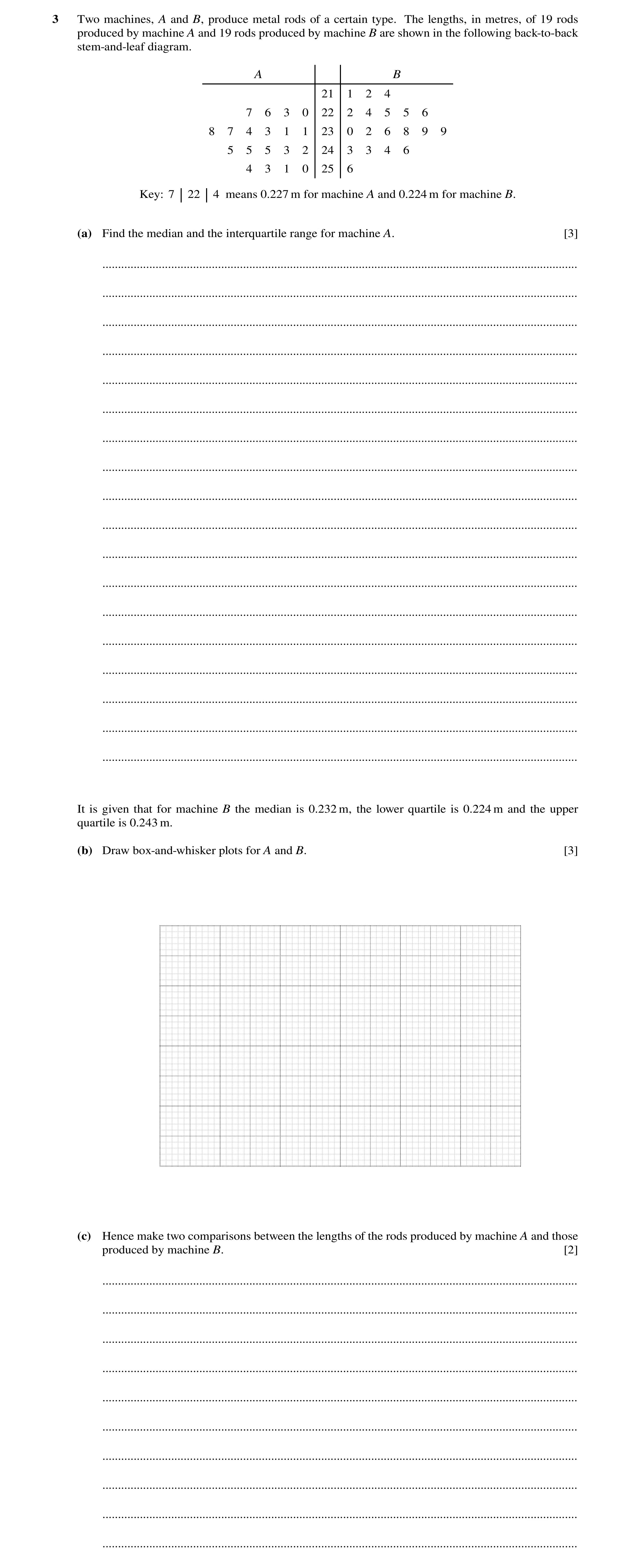
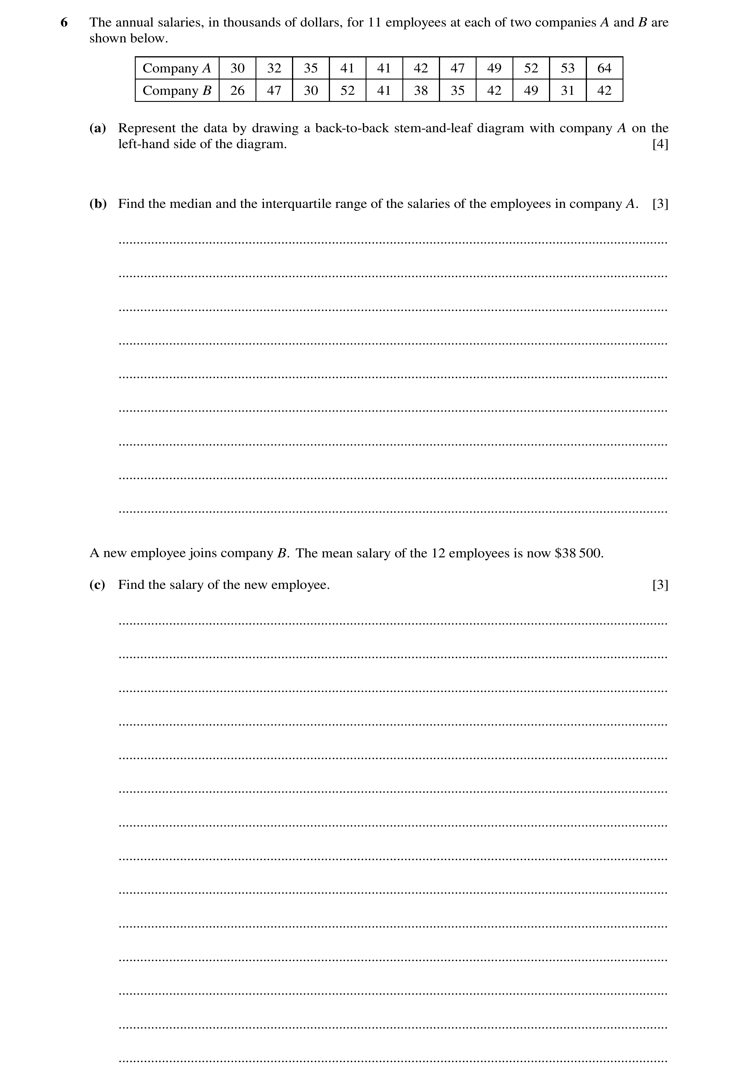
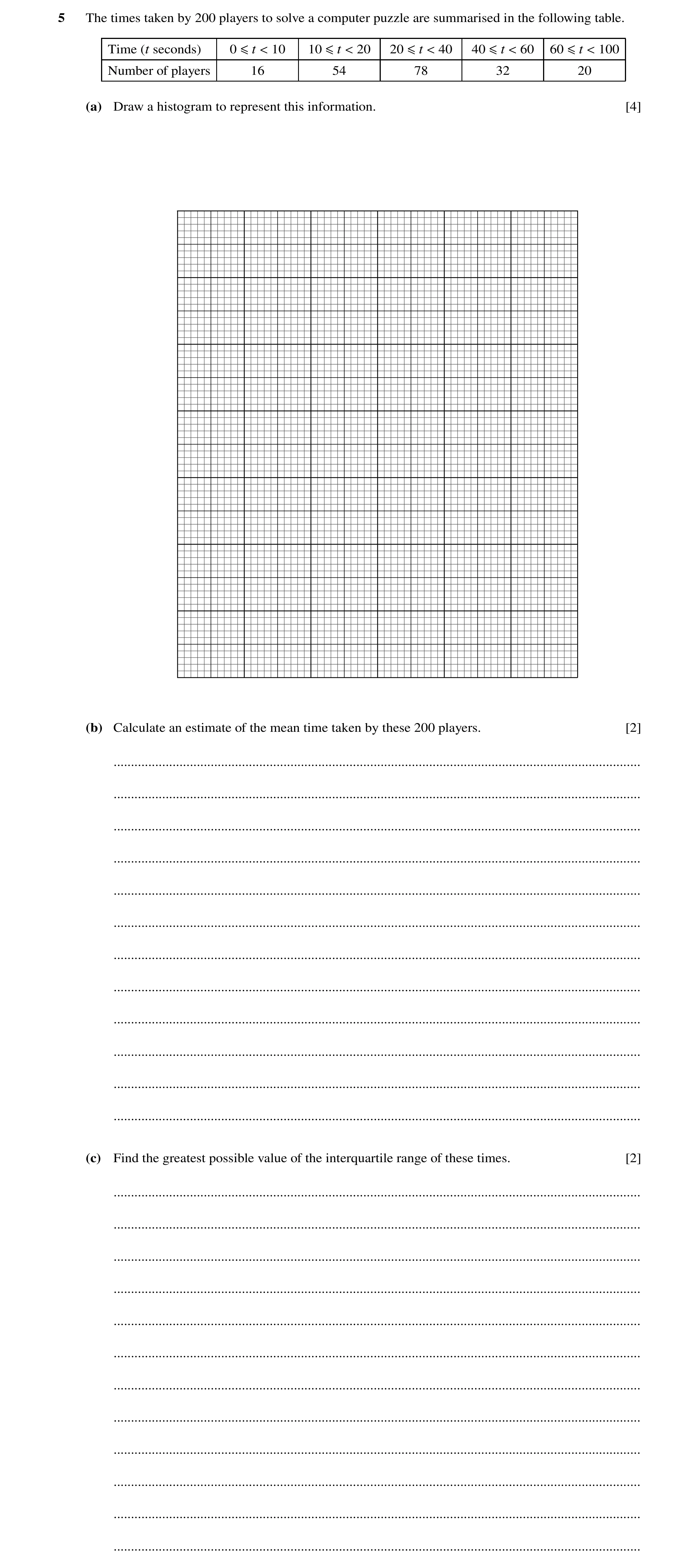
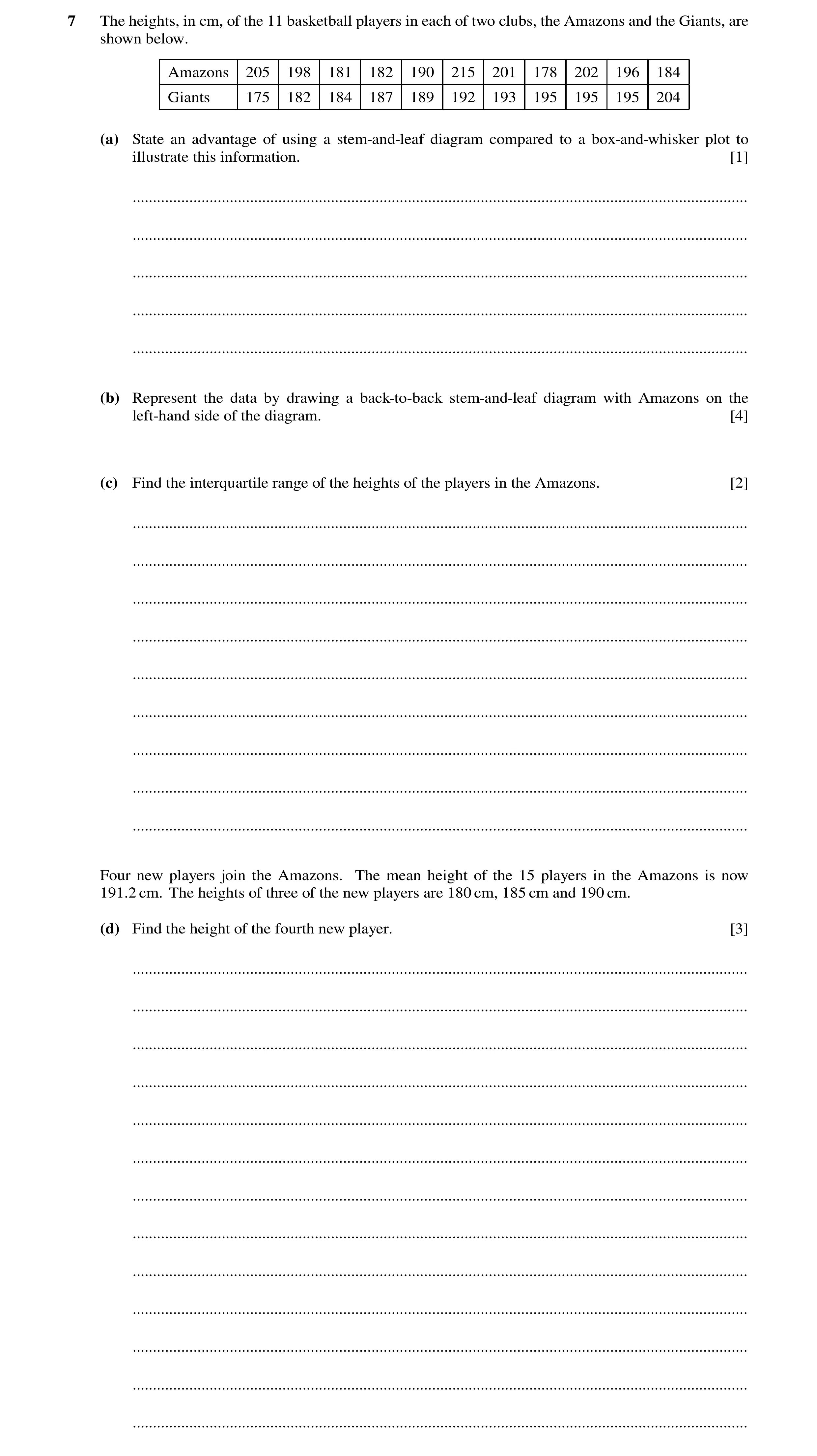
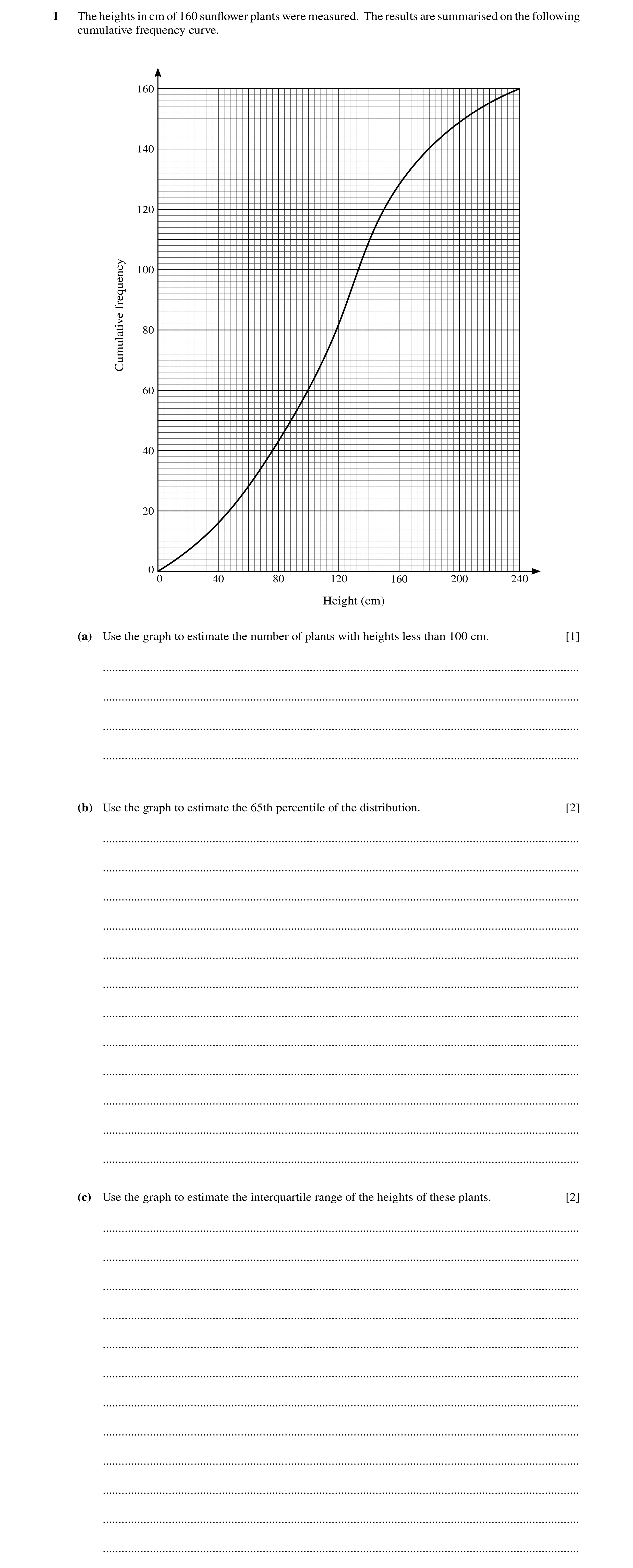
 20 / 83
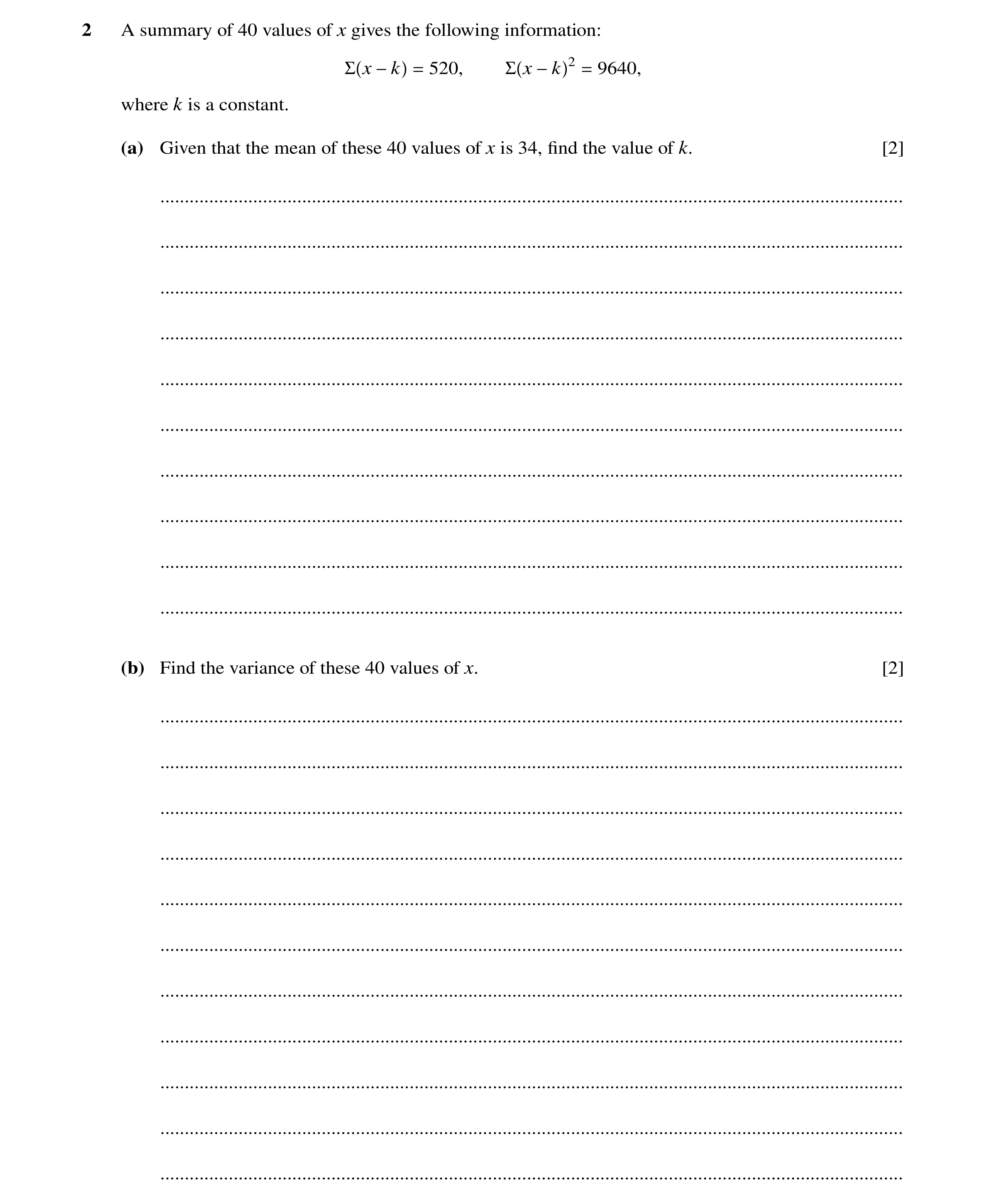 21 / 83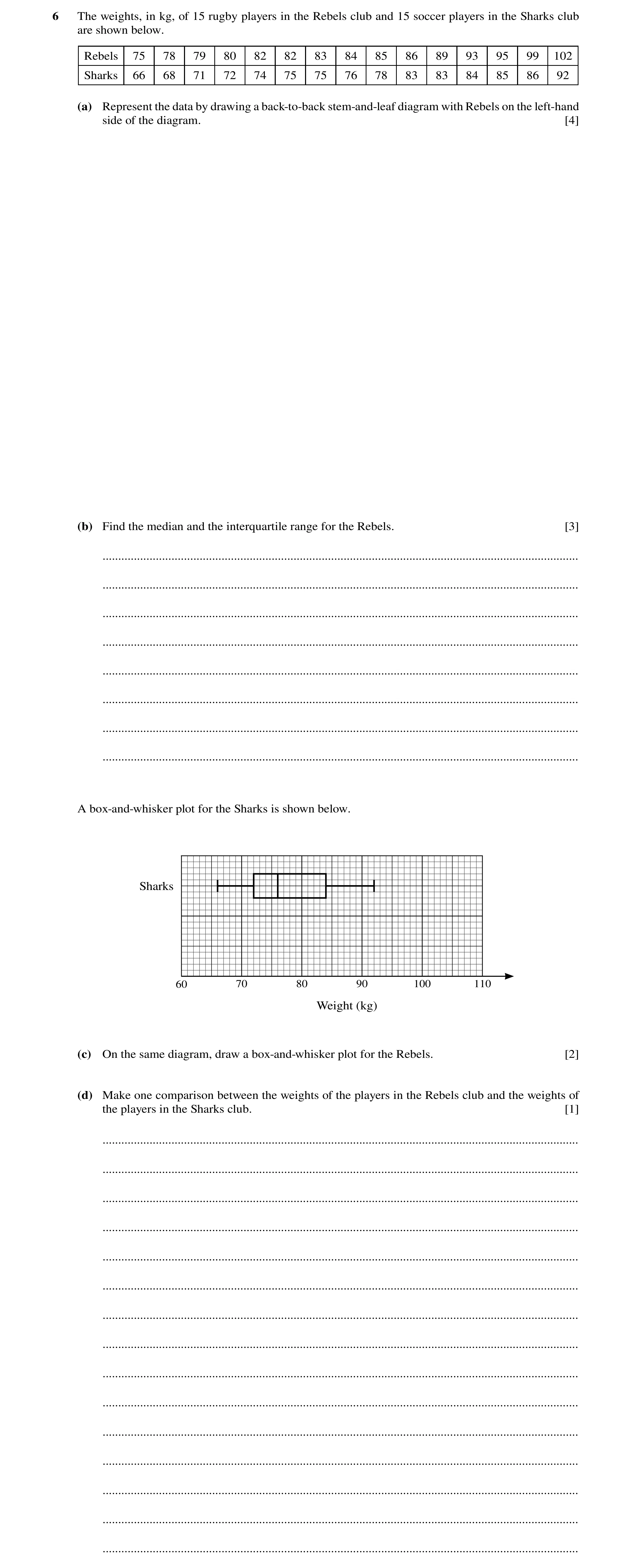
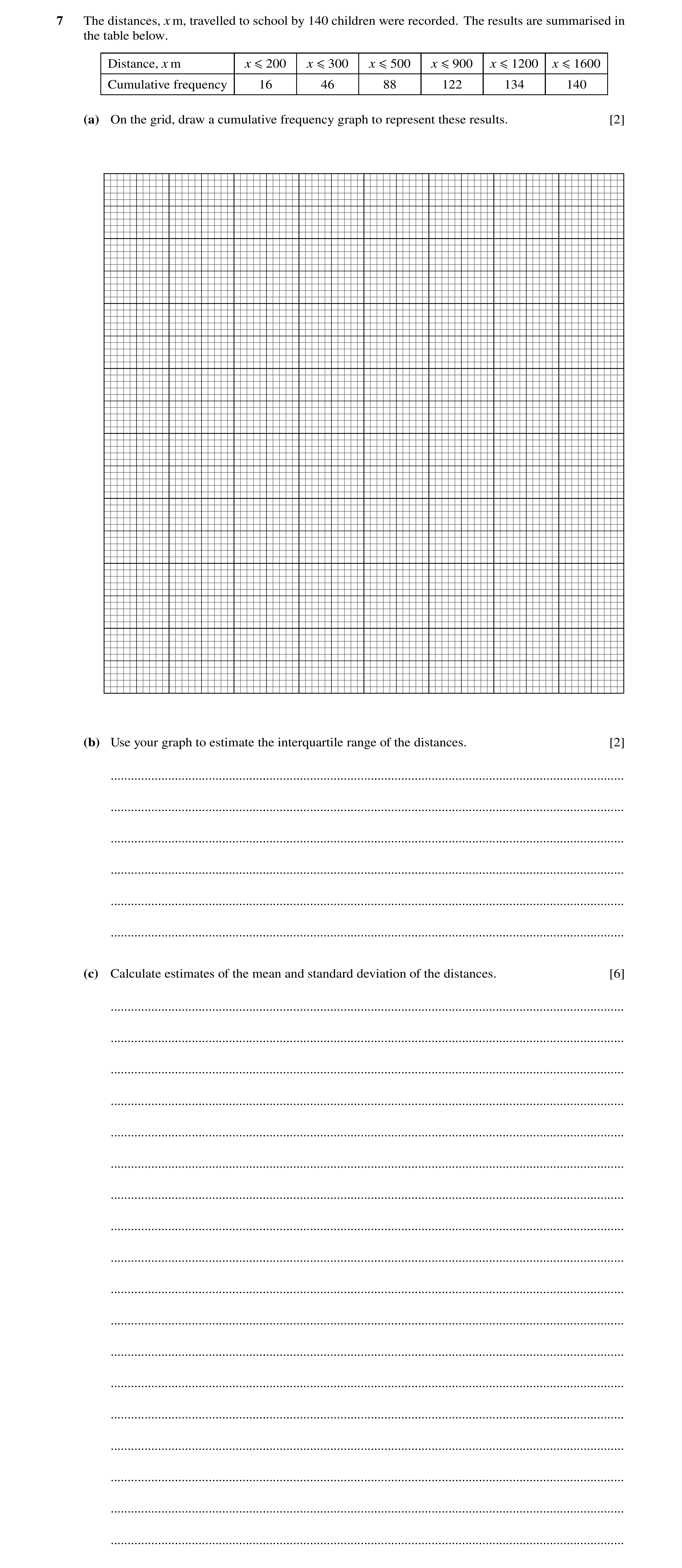
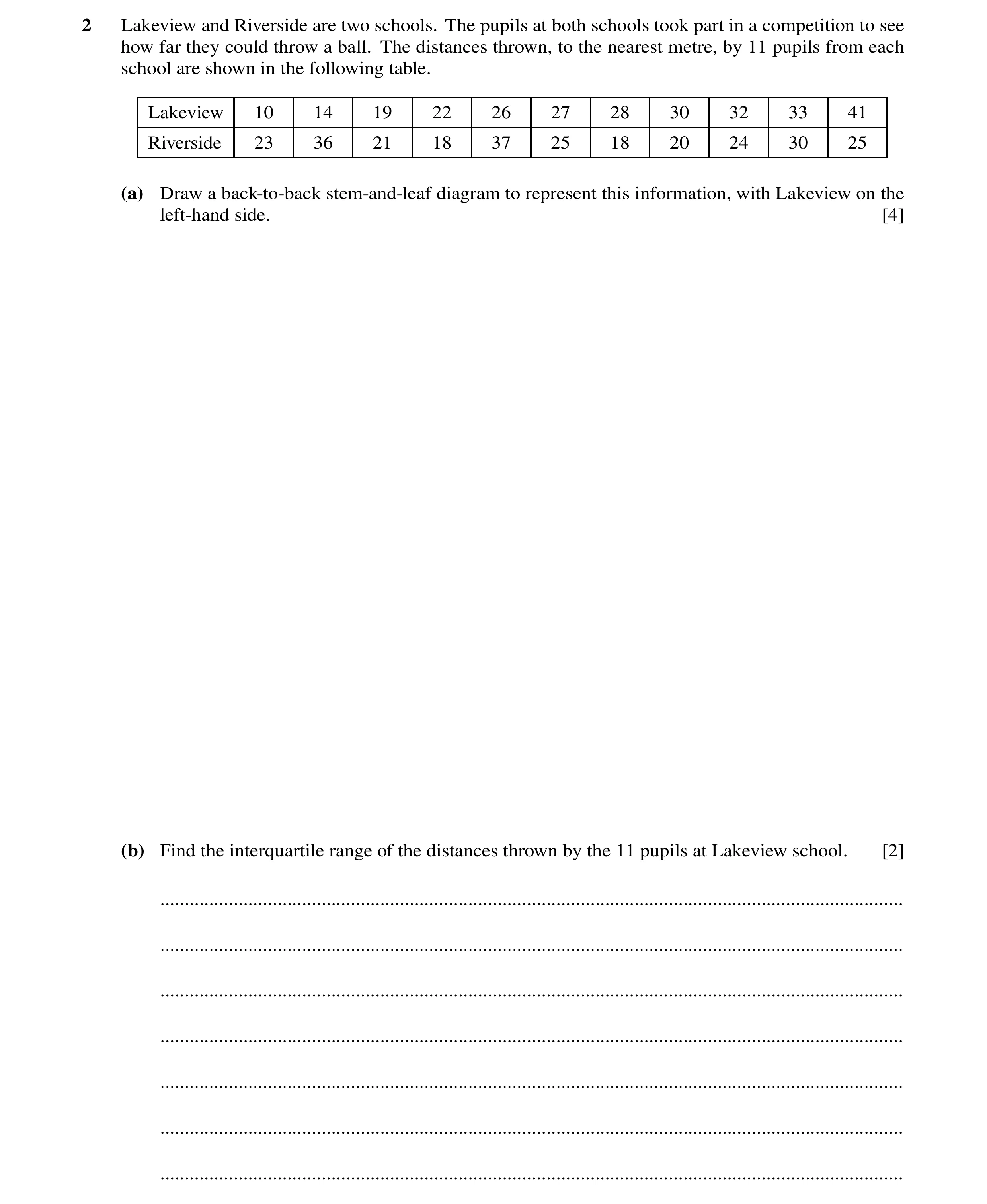 26 / 83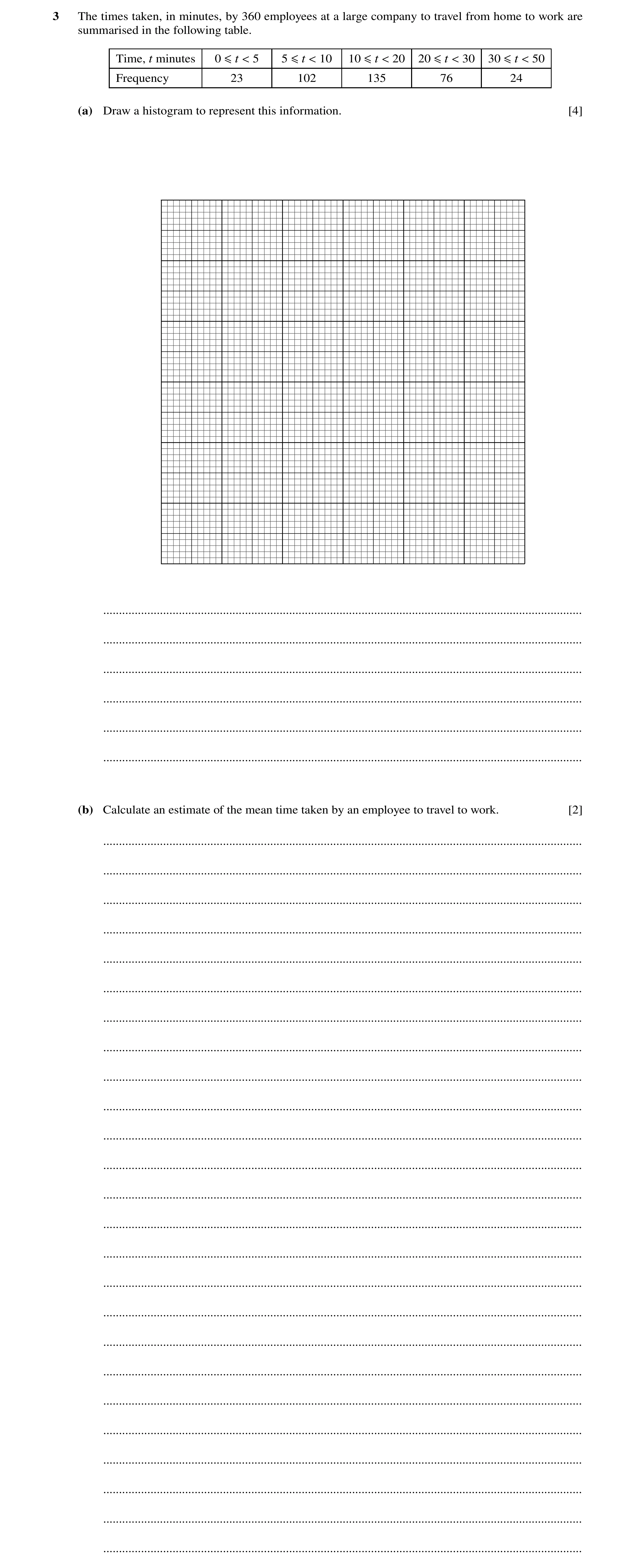
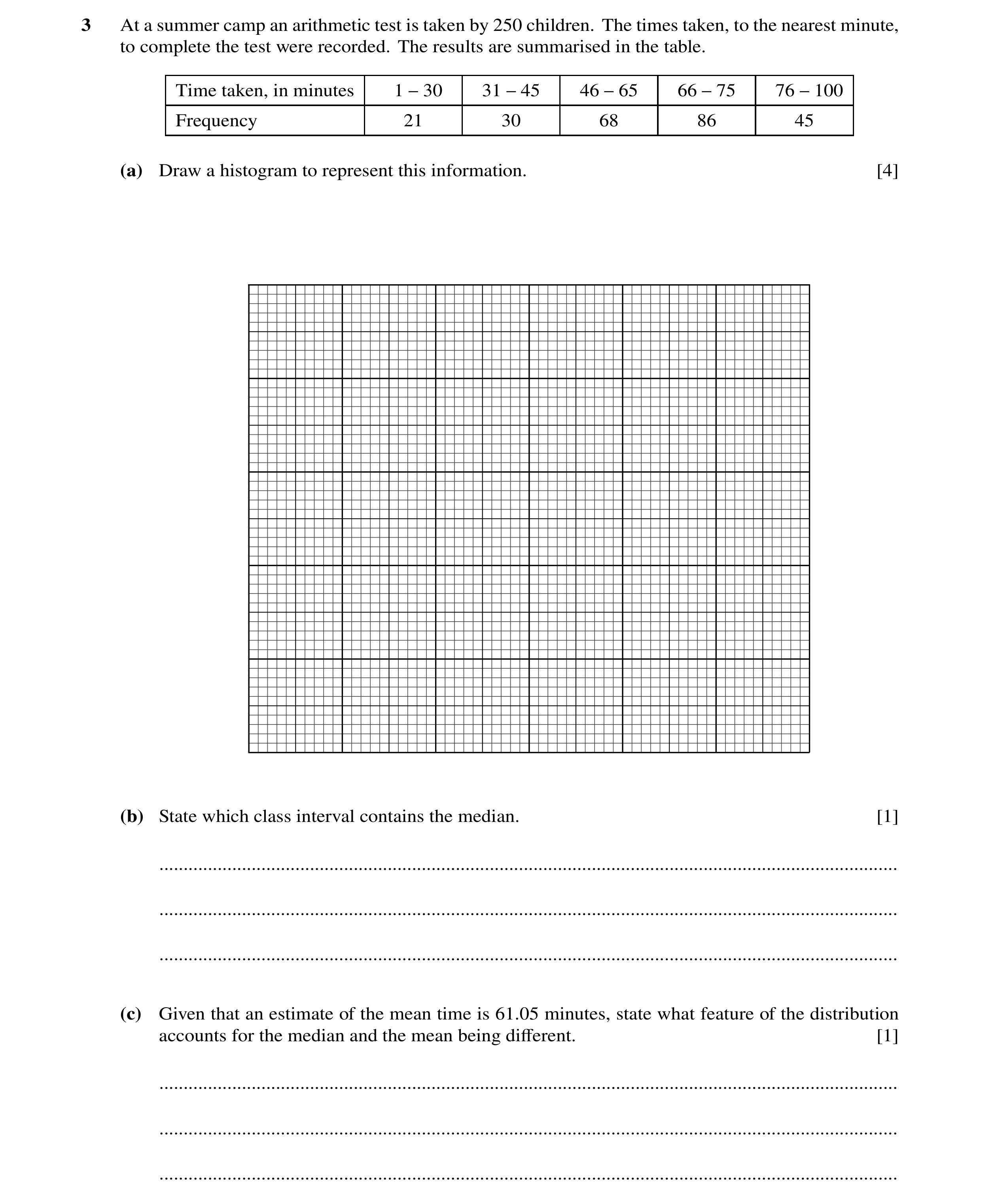 29 / 83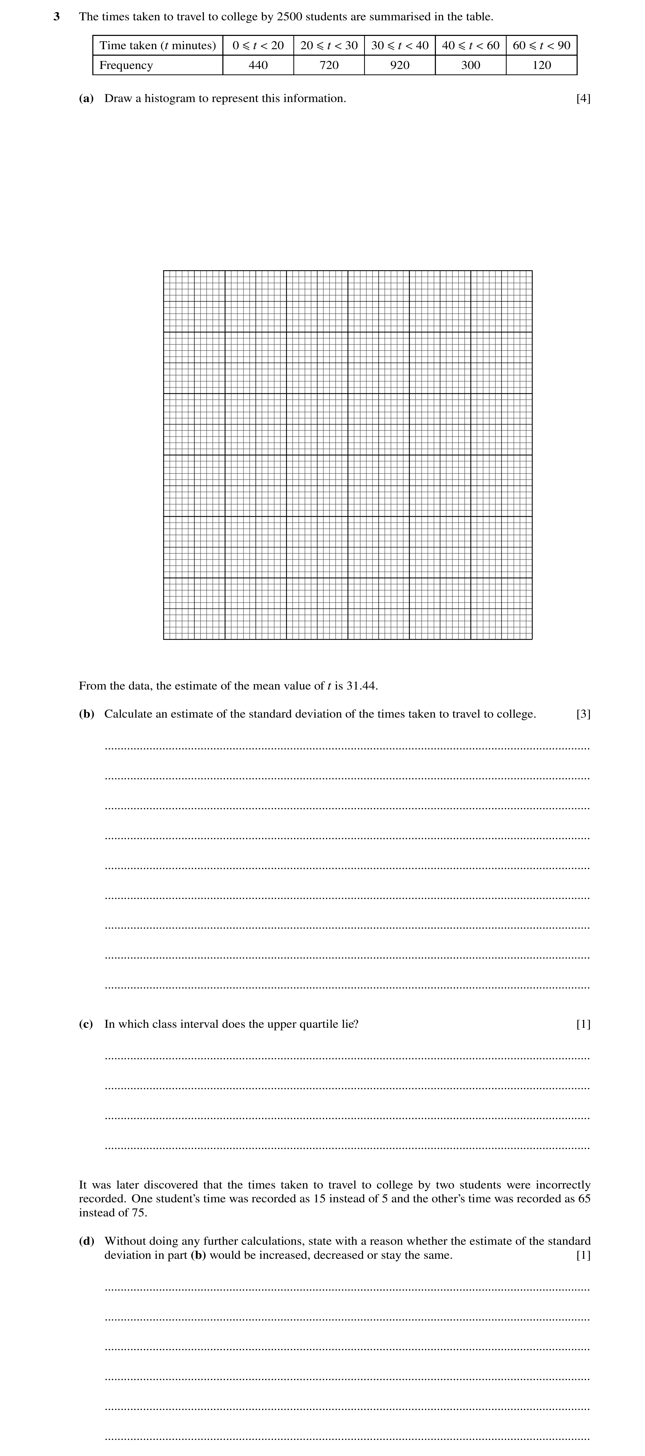
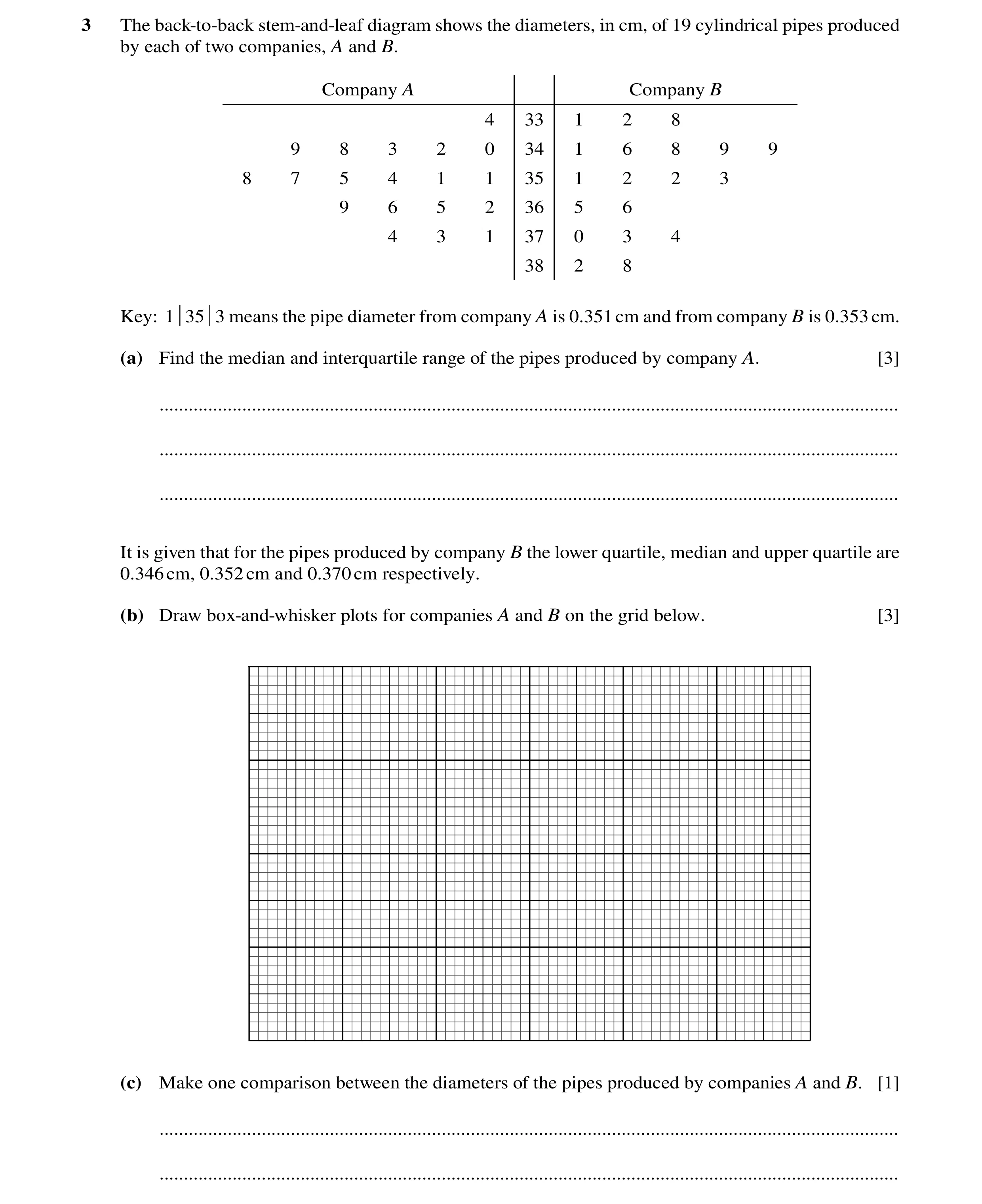 32 / 83
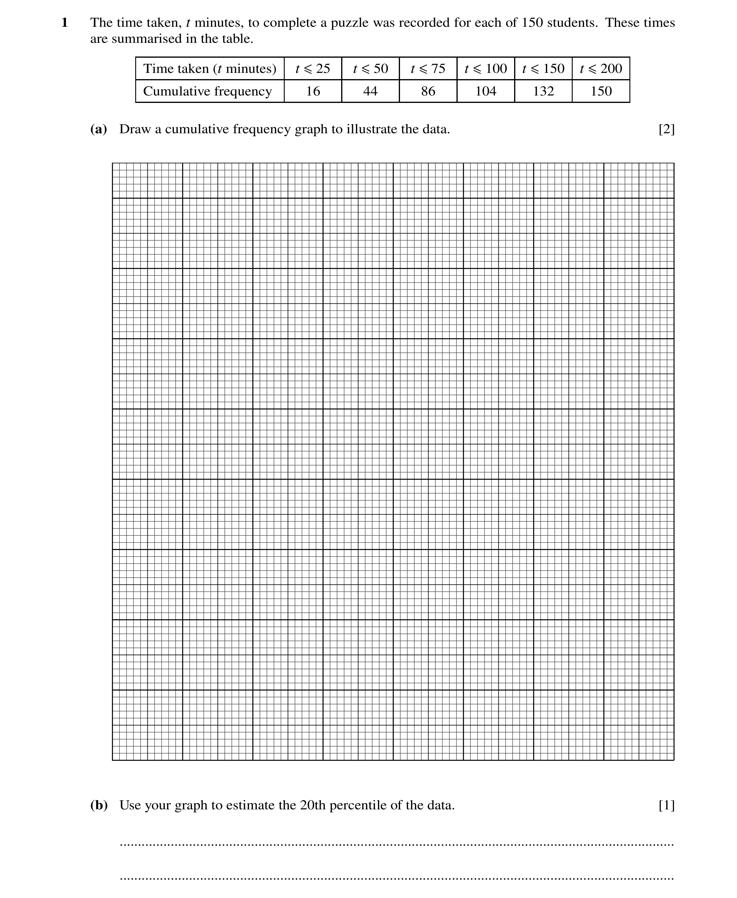 33 / 83
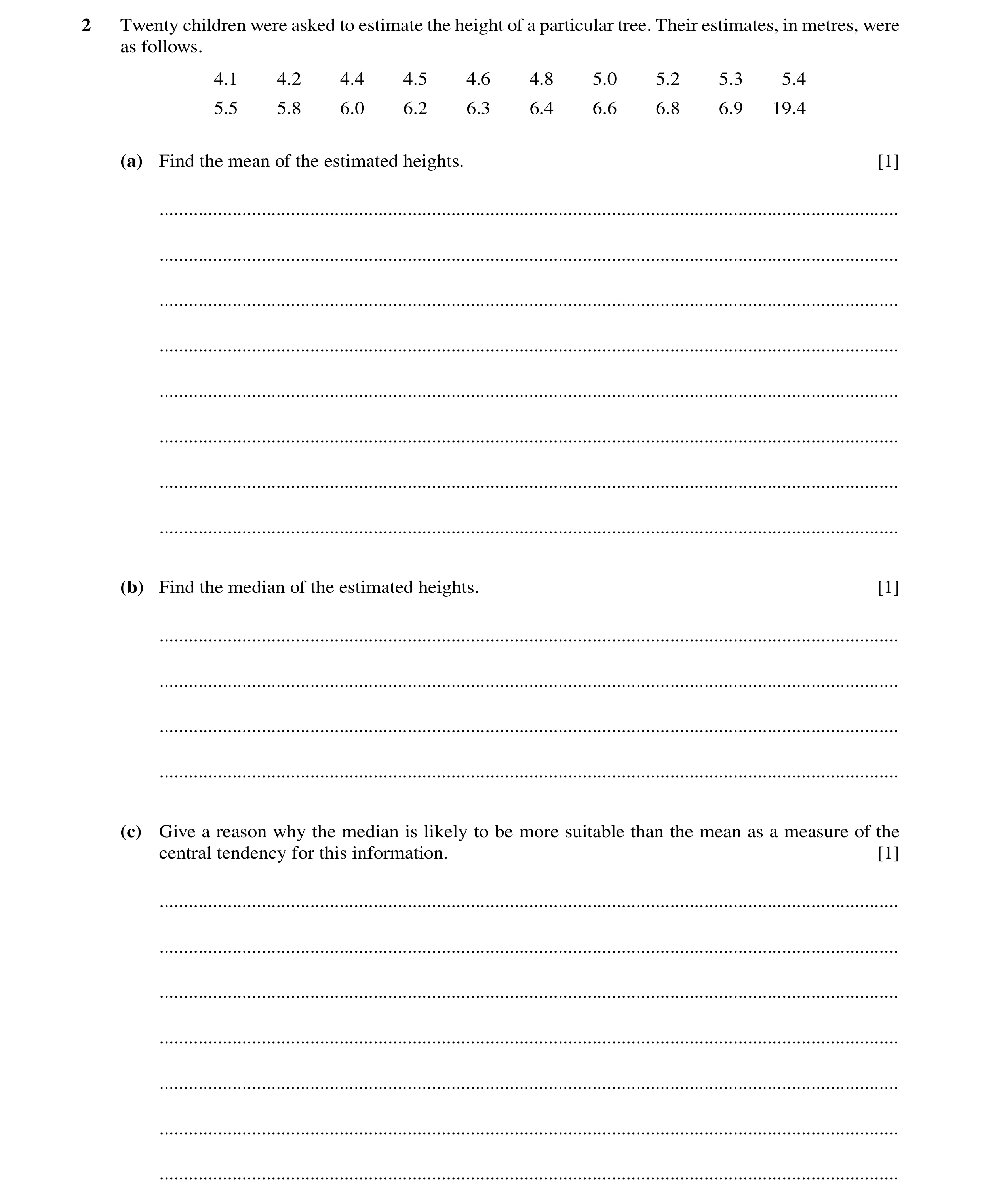 34 / 83
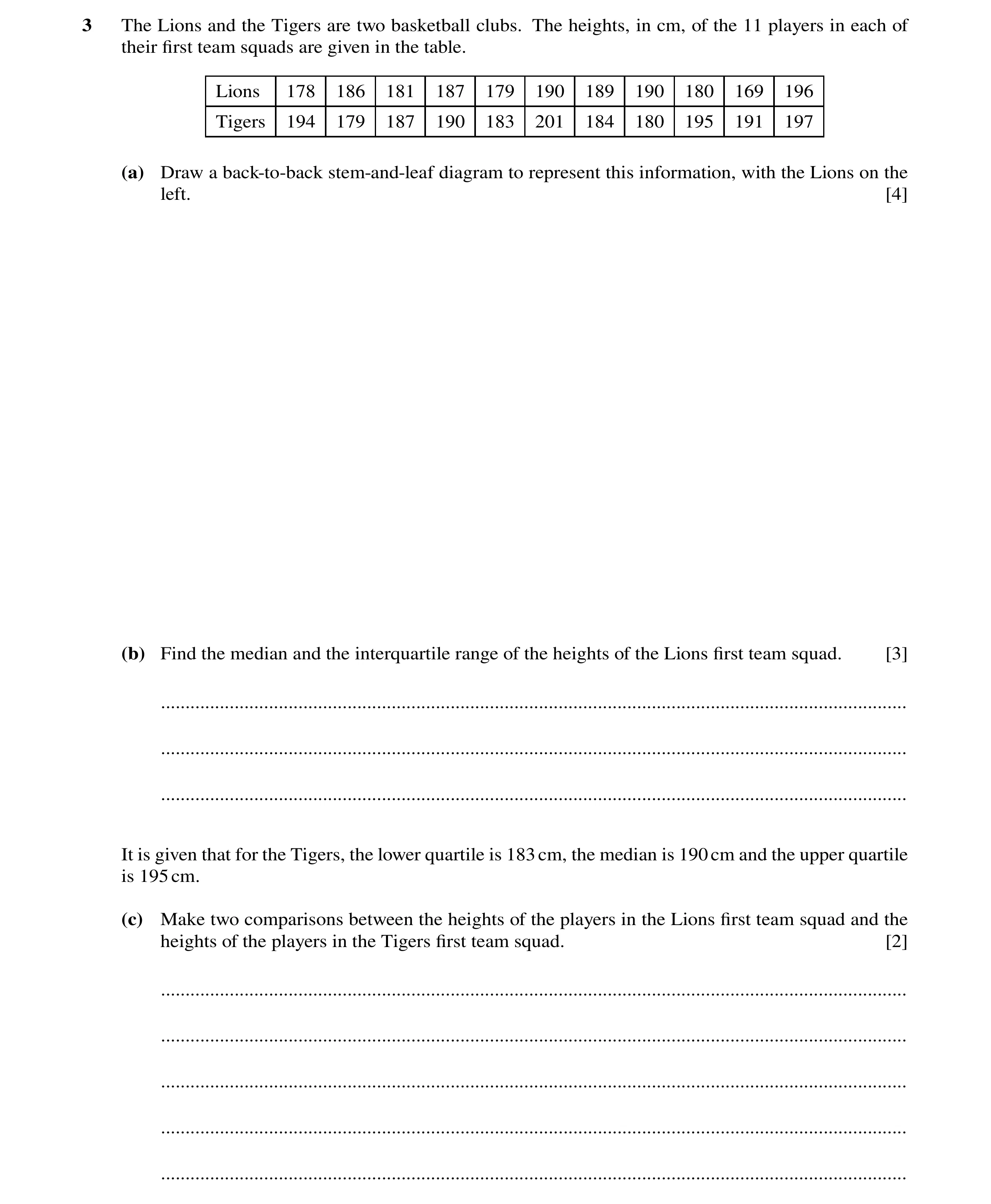 35 / 83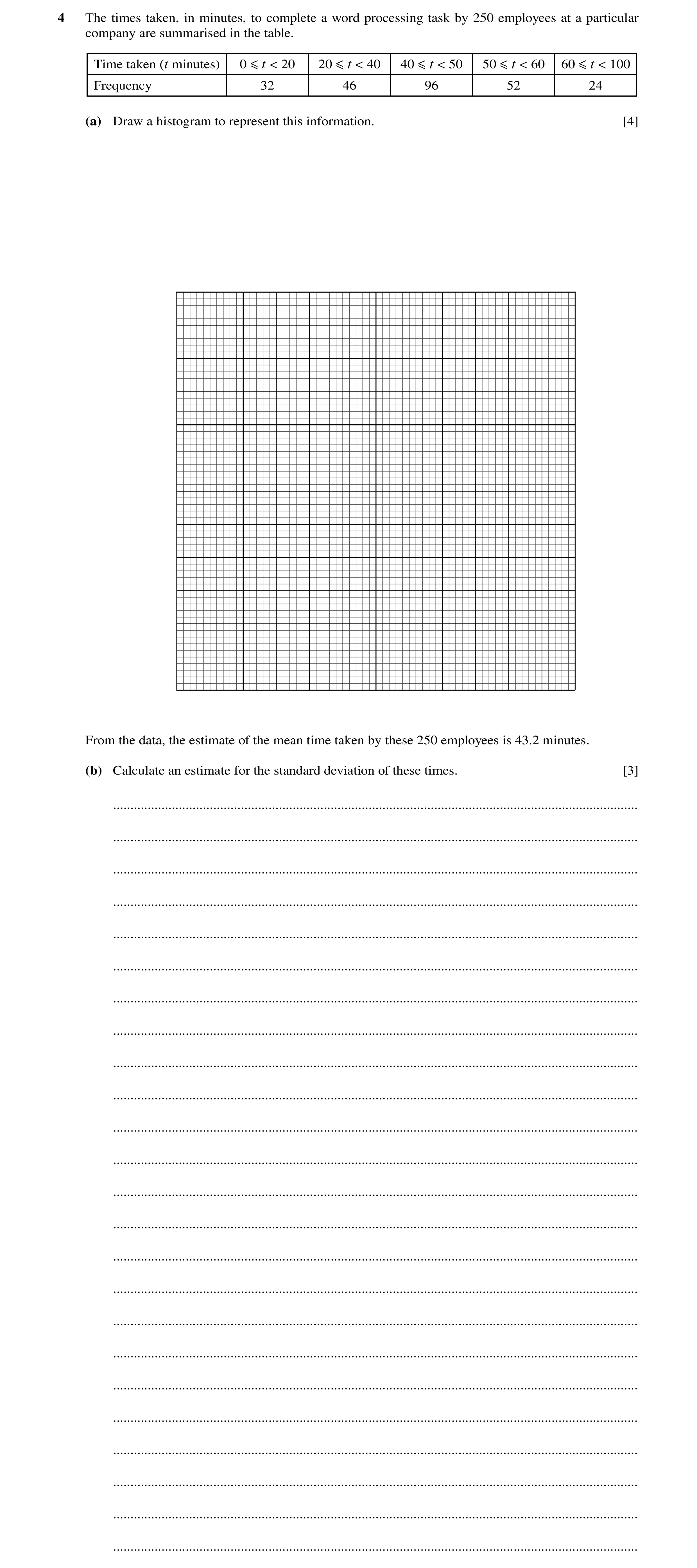
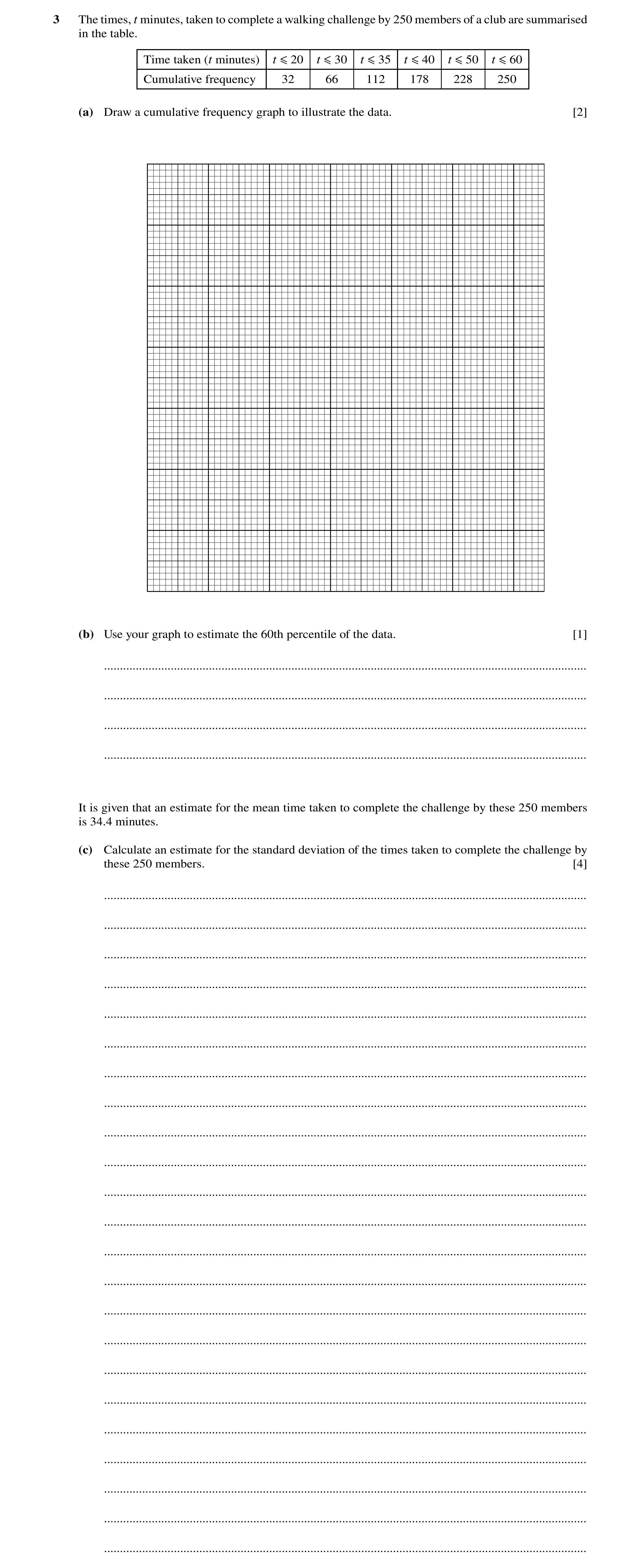
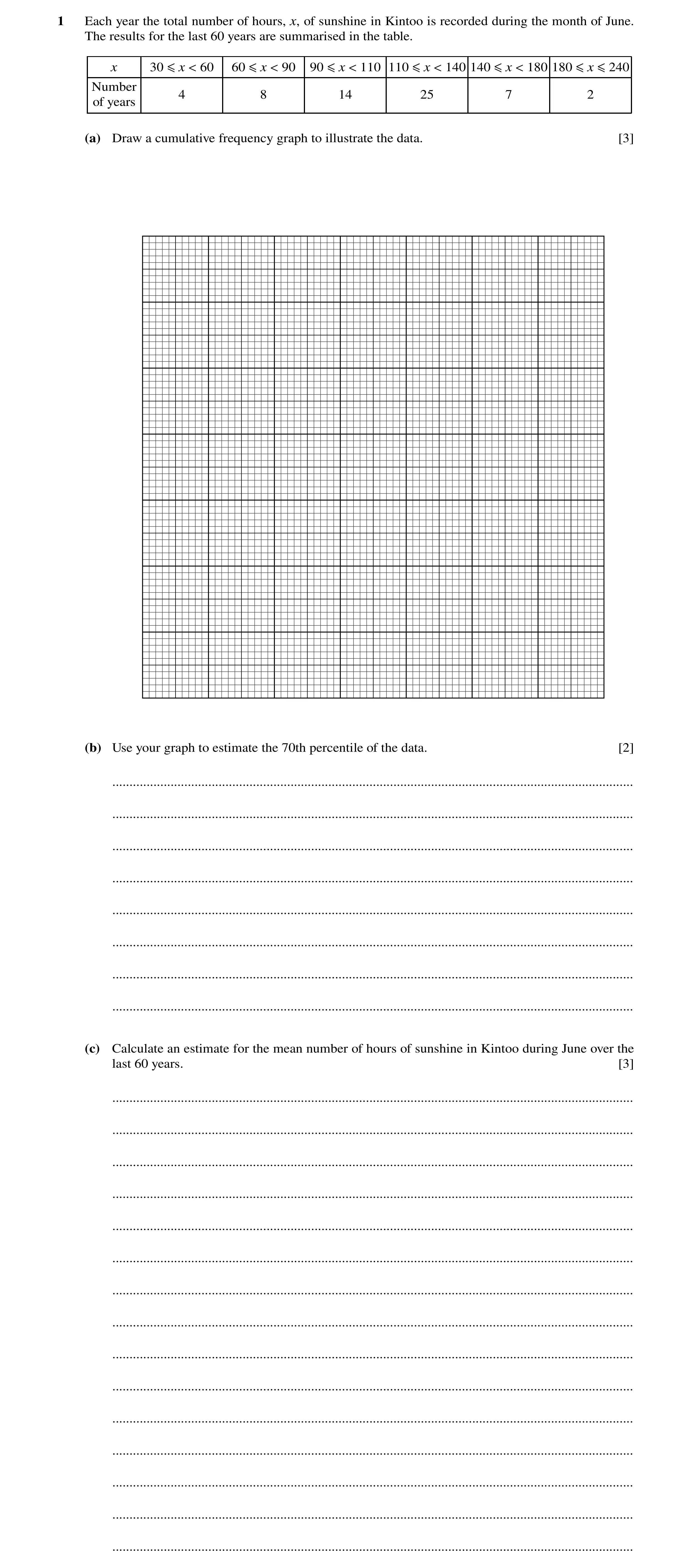
 42 / 83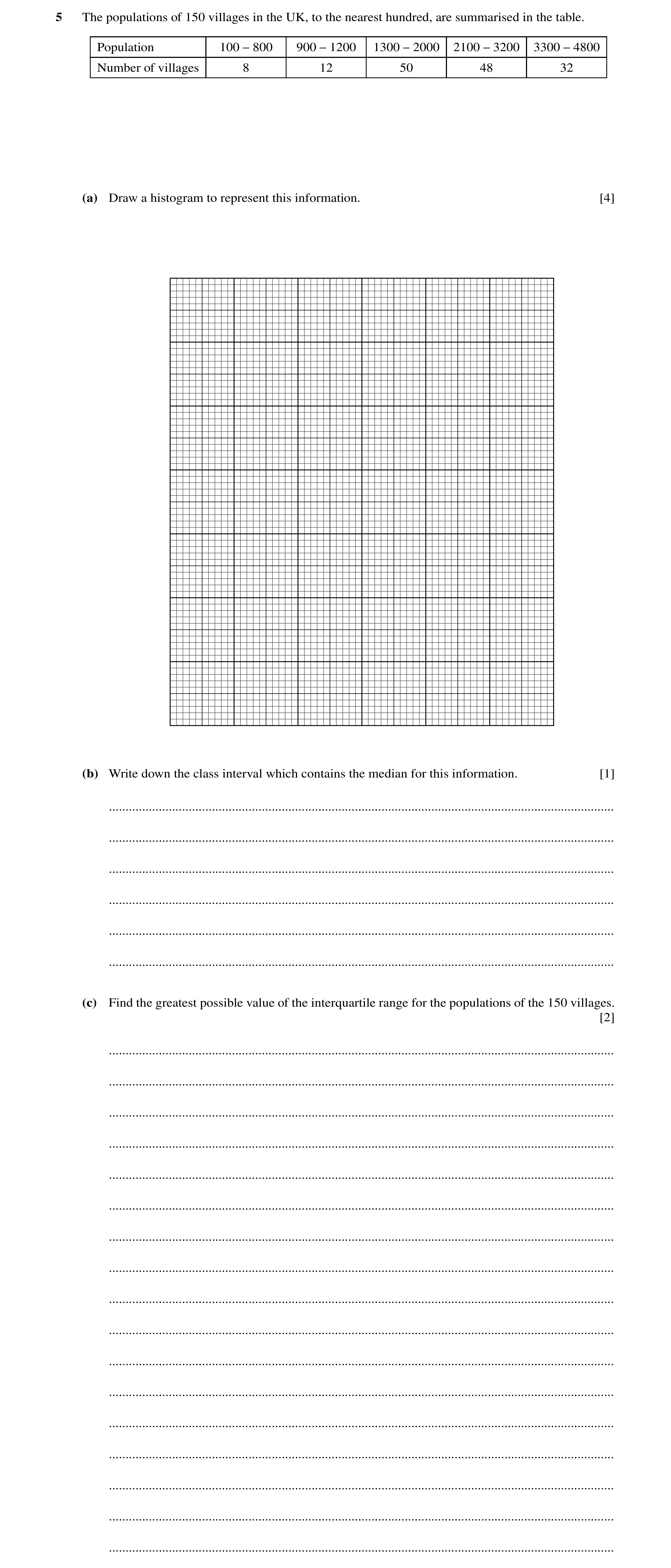
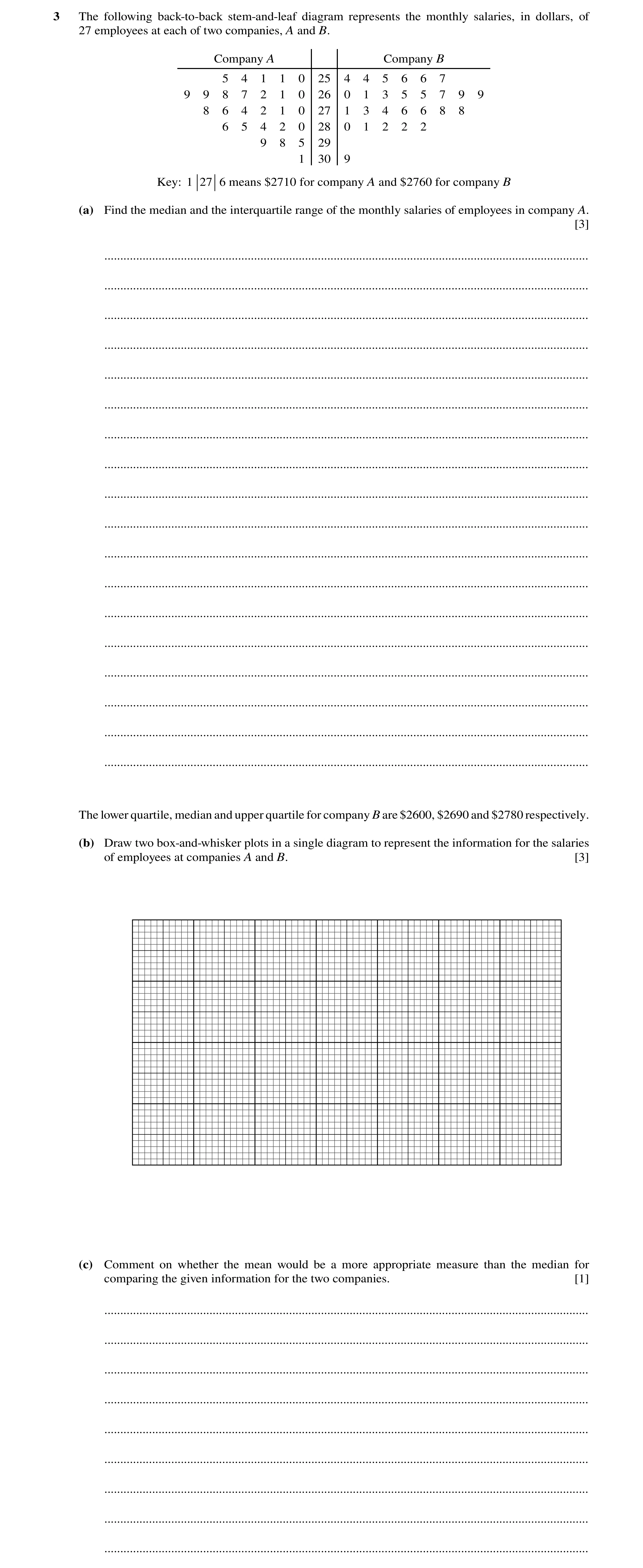
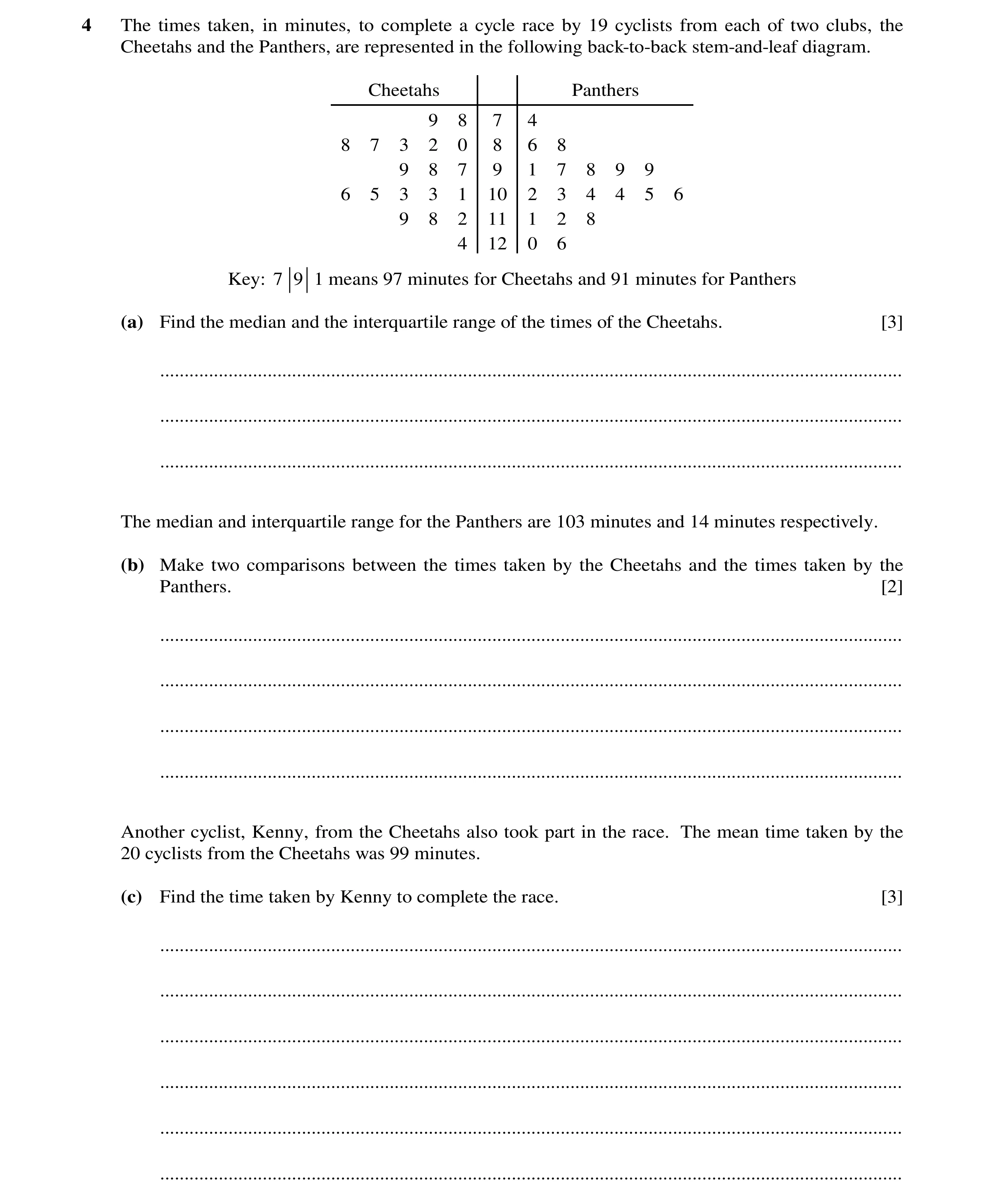 47 / 83
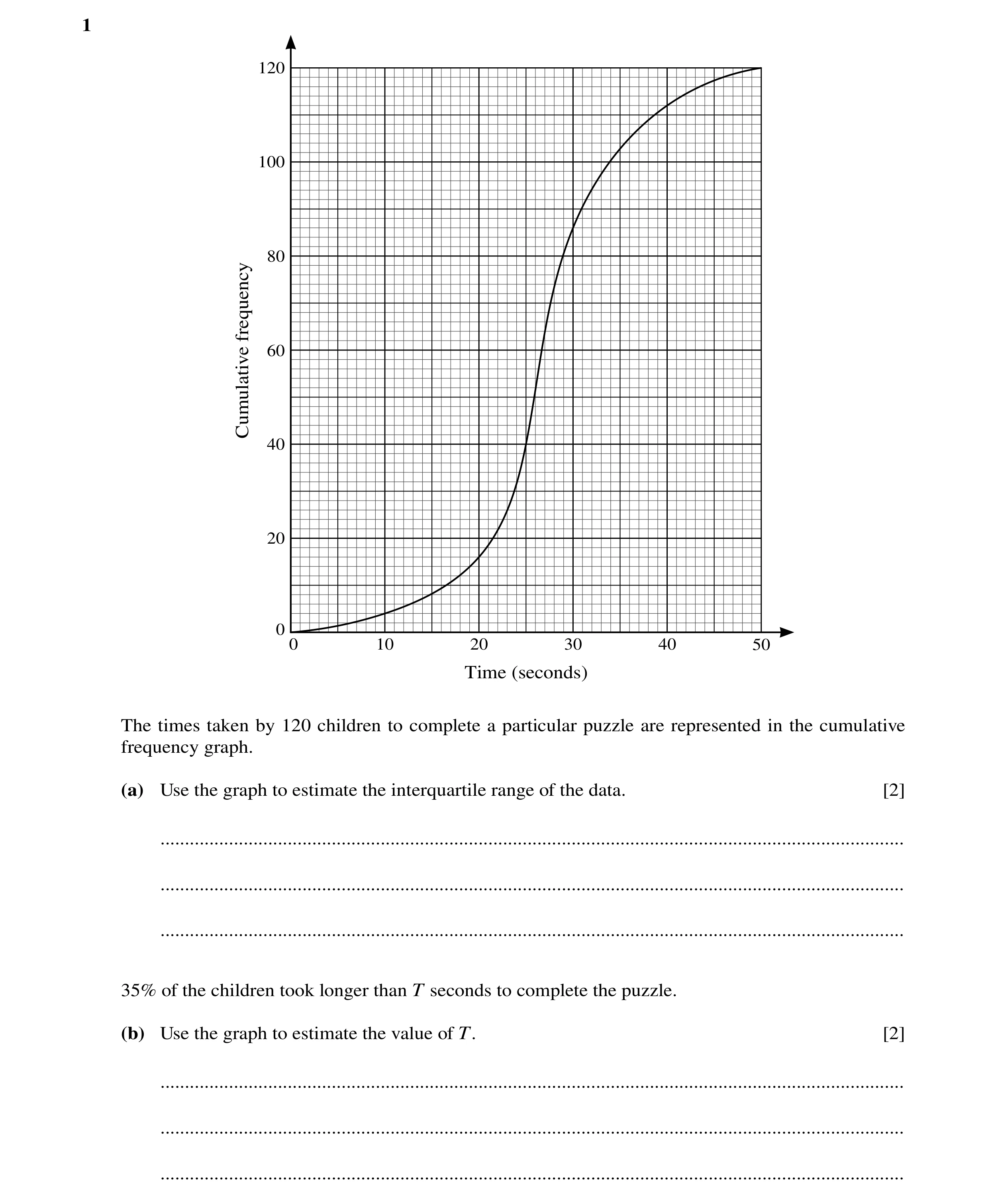 48 / 83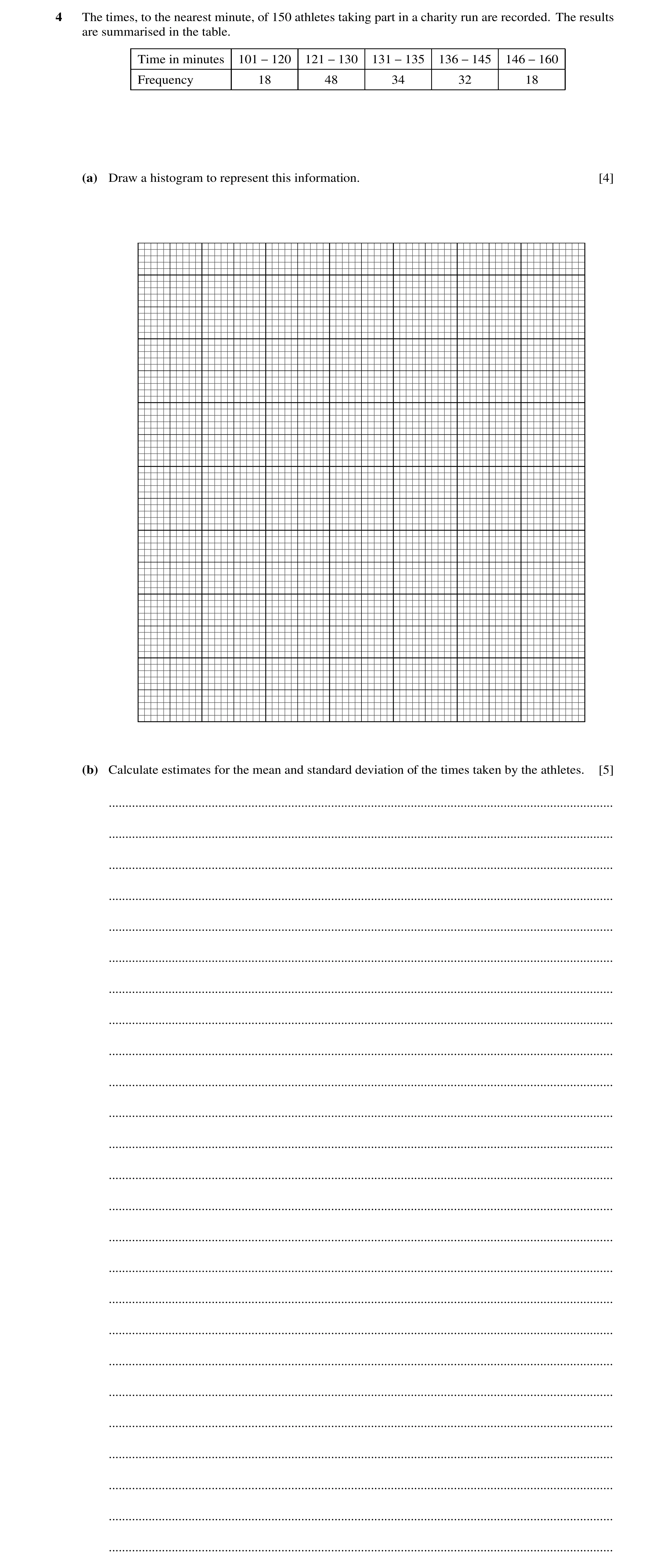
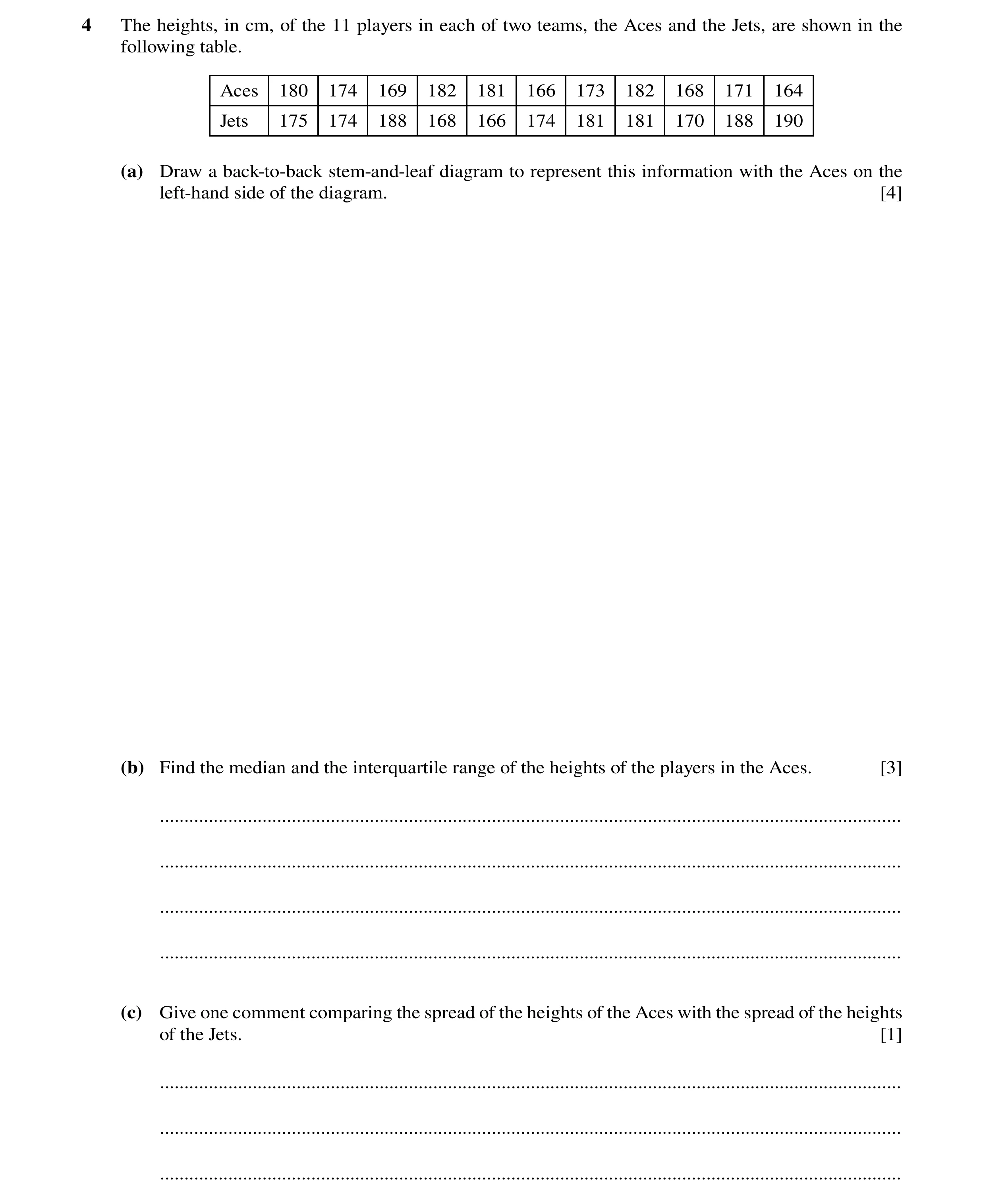 51 / 83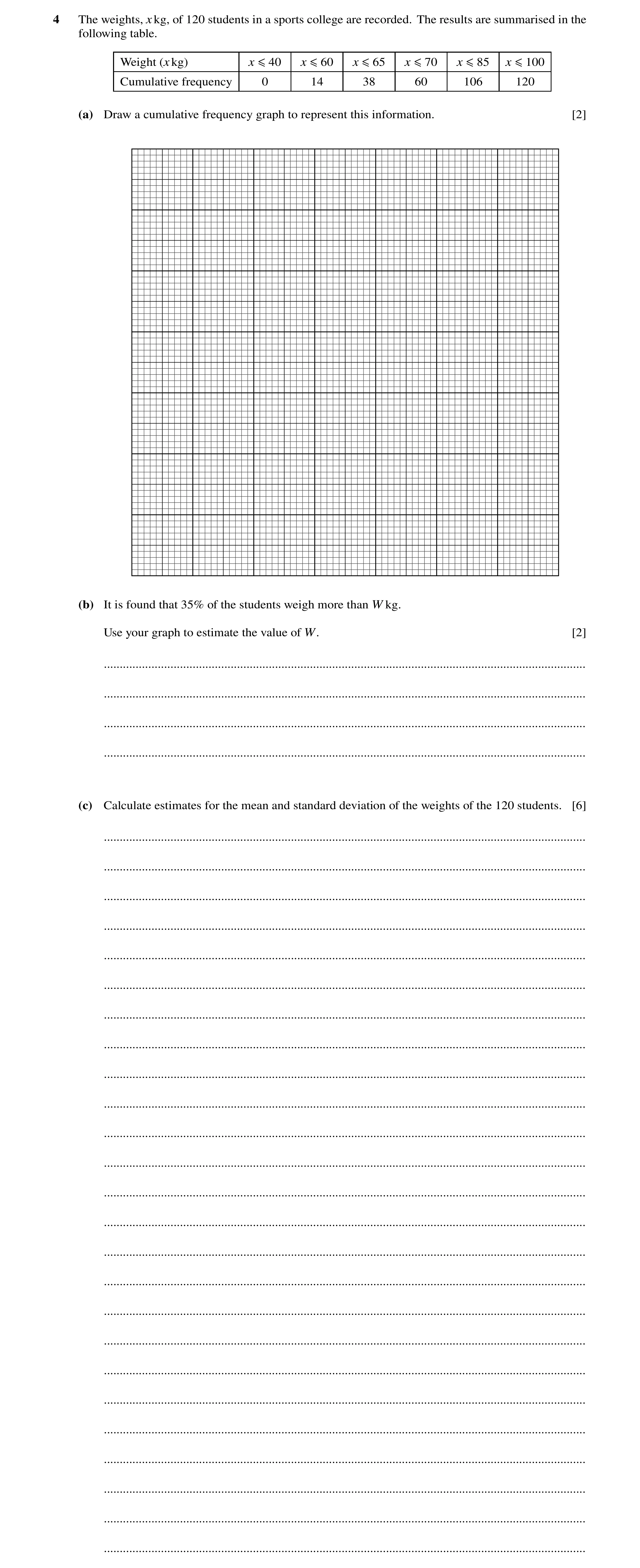
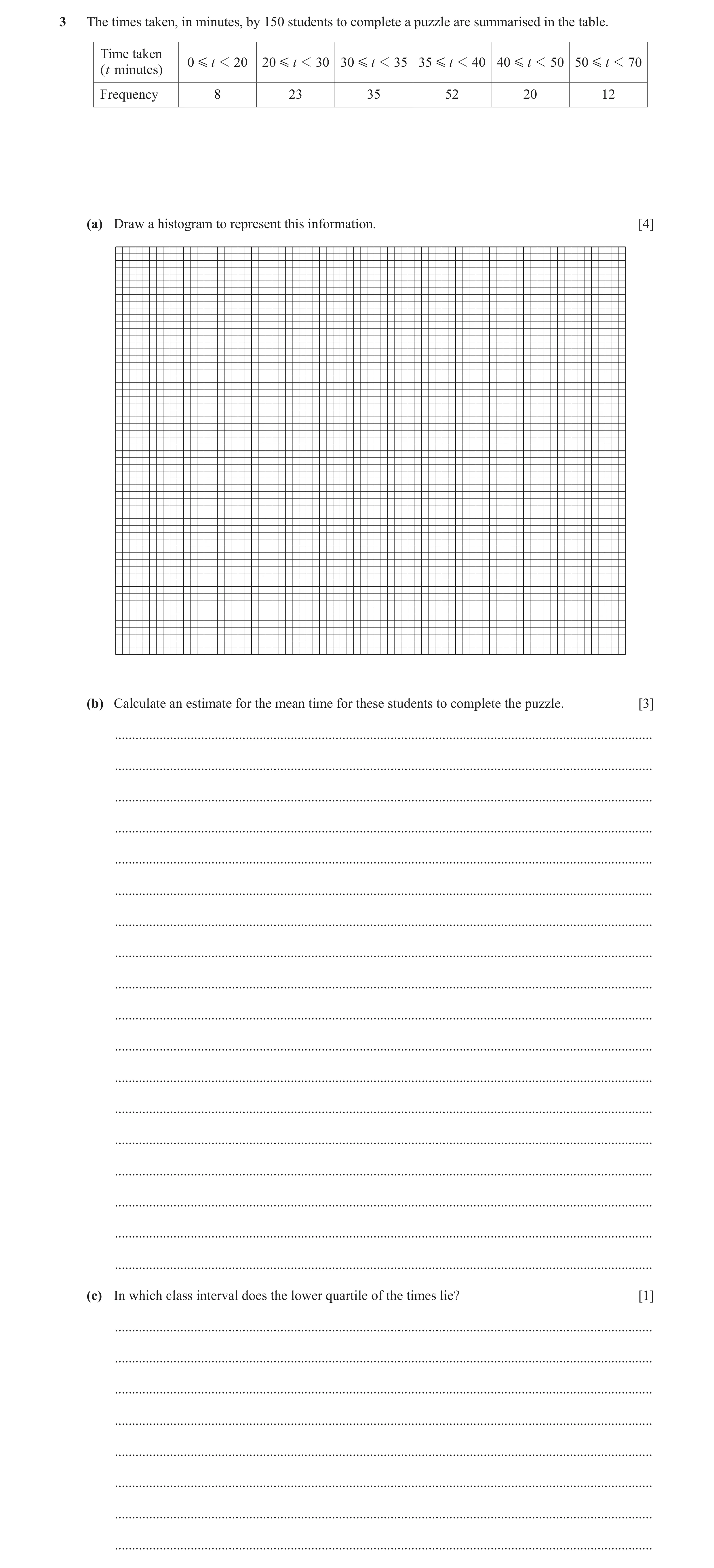
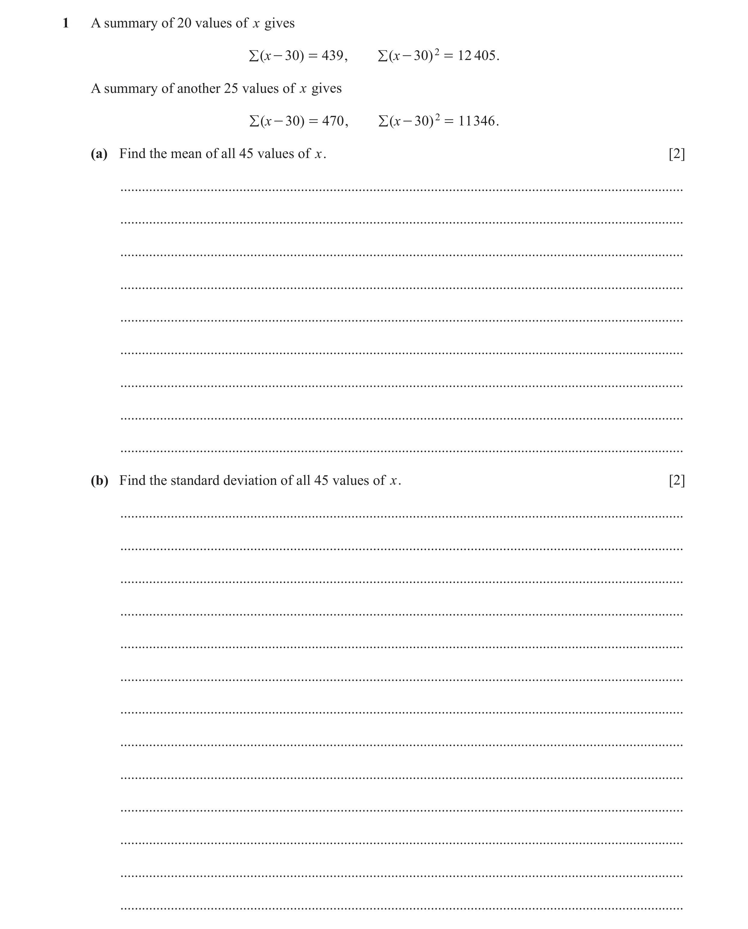 56 / 83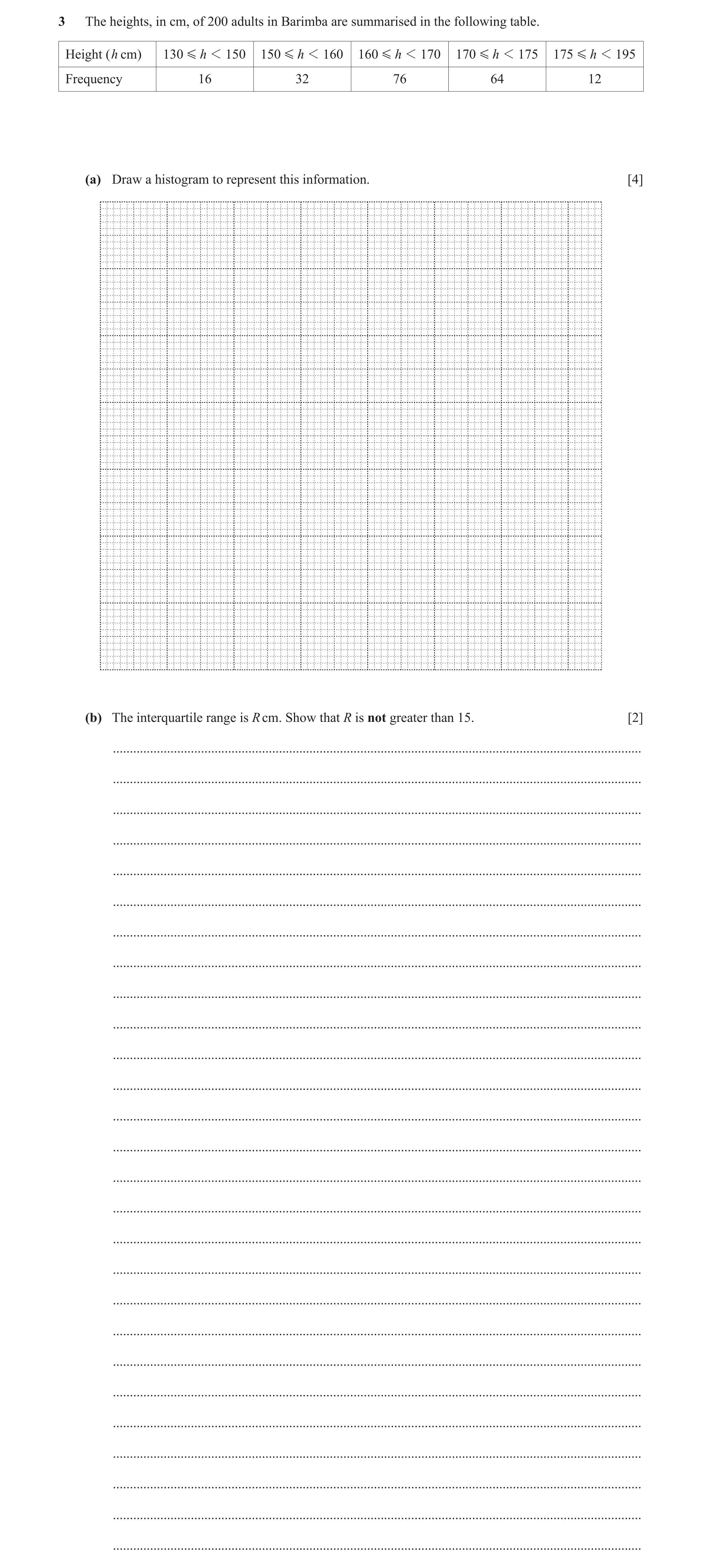
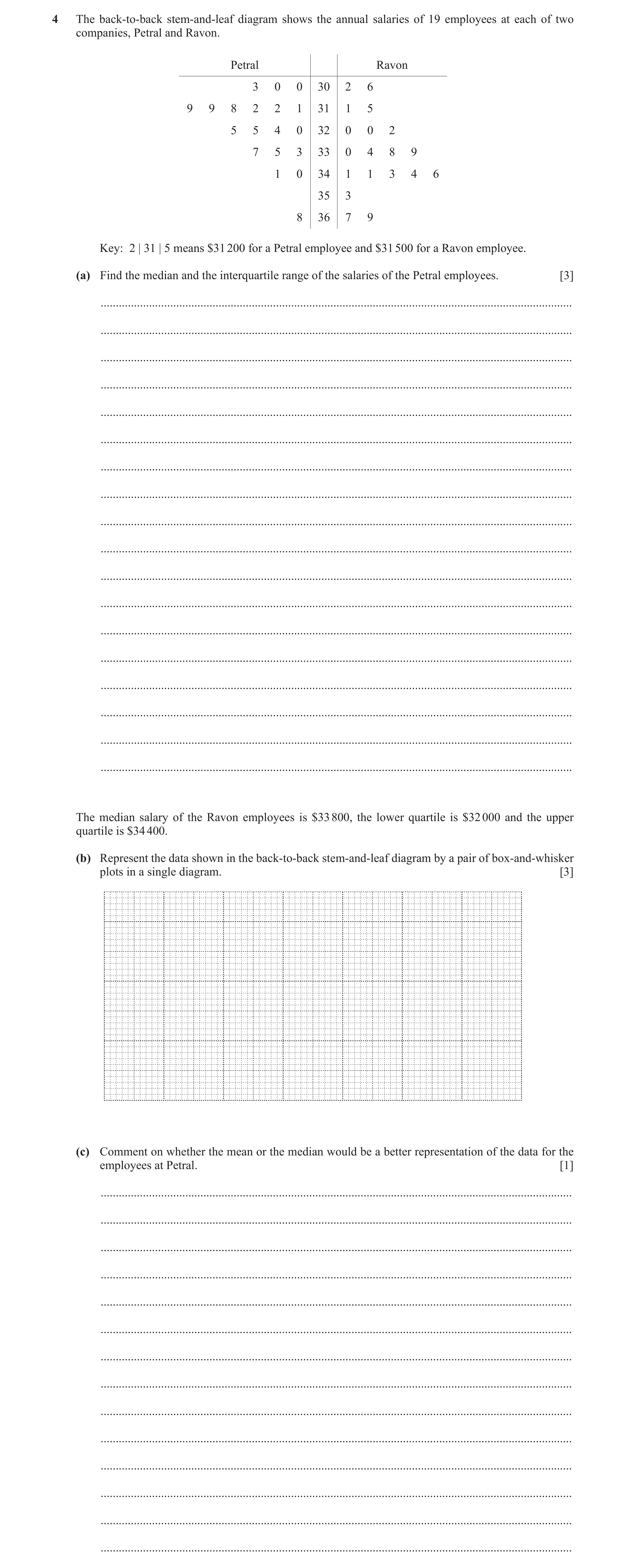
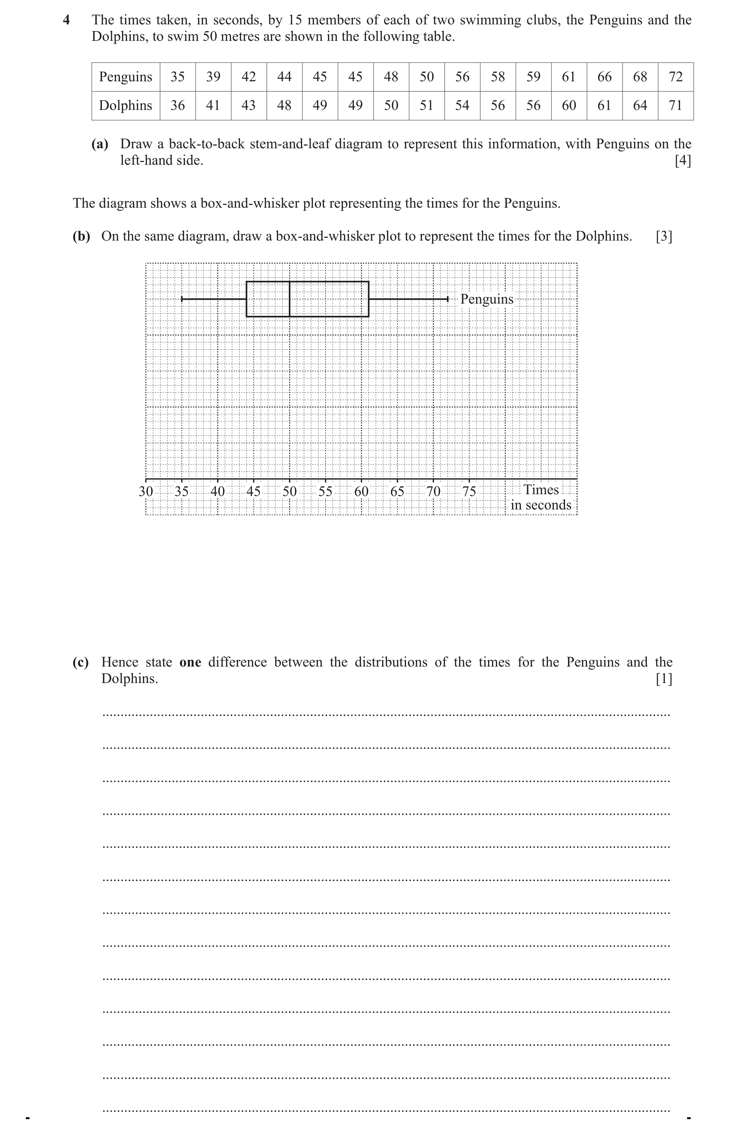
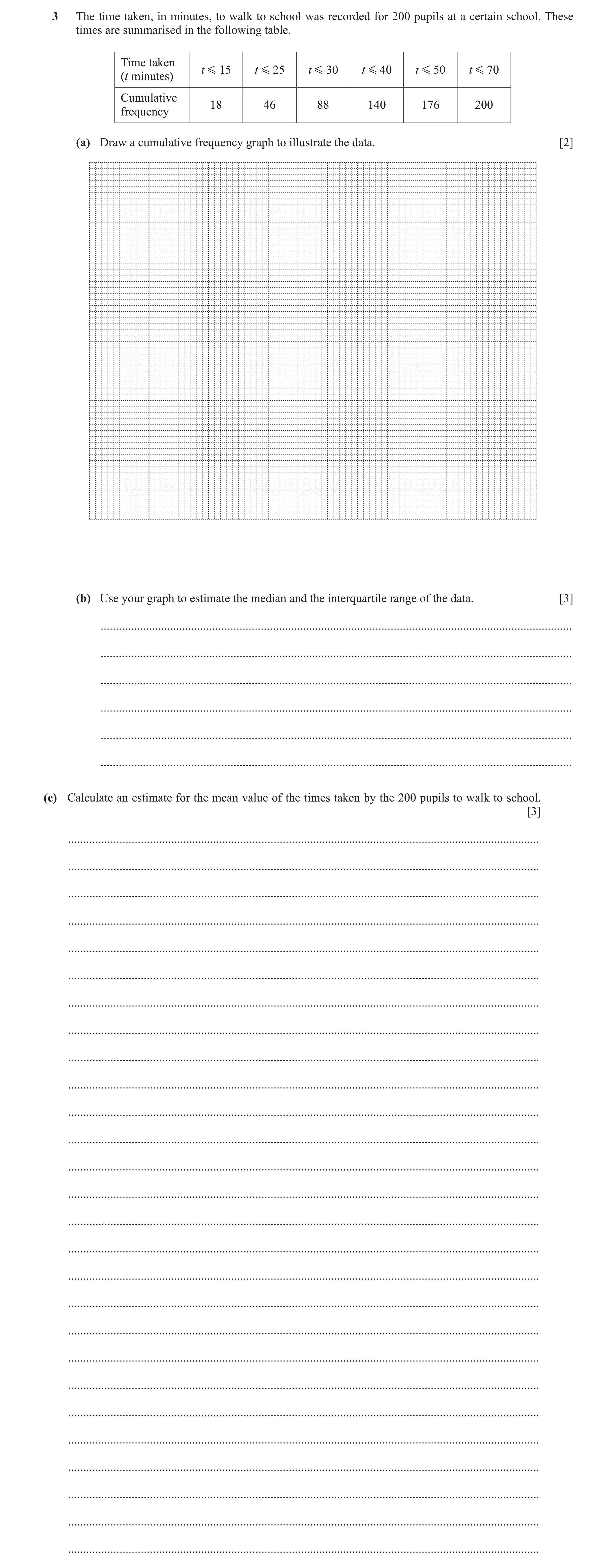
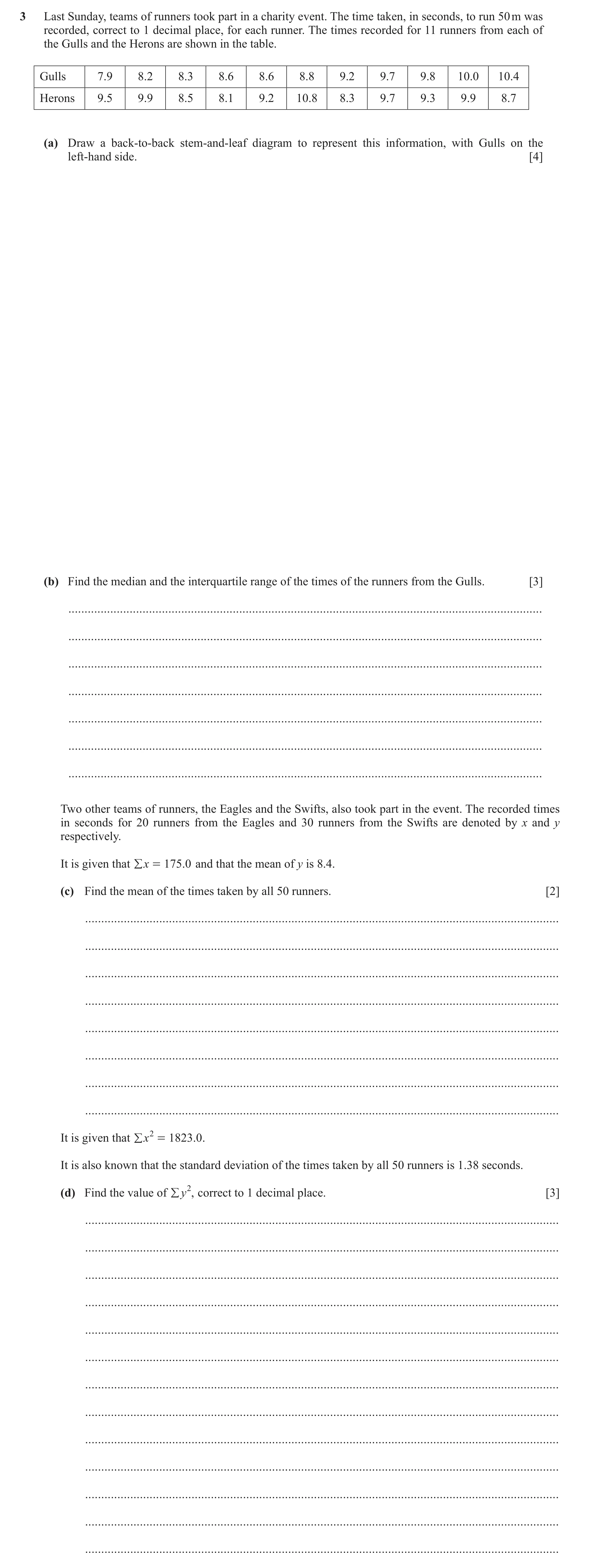
 72 / 83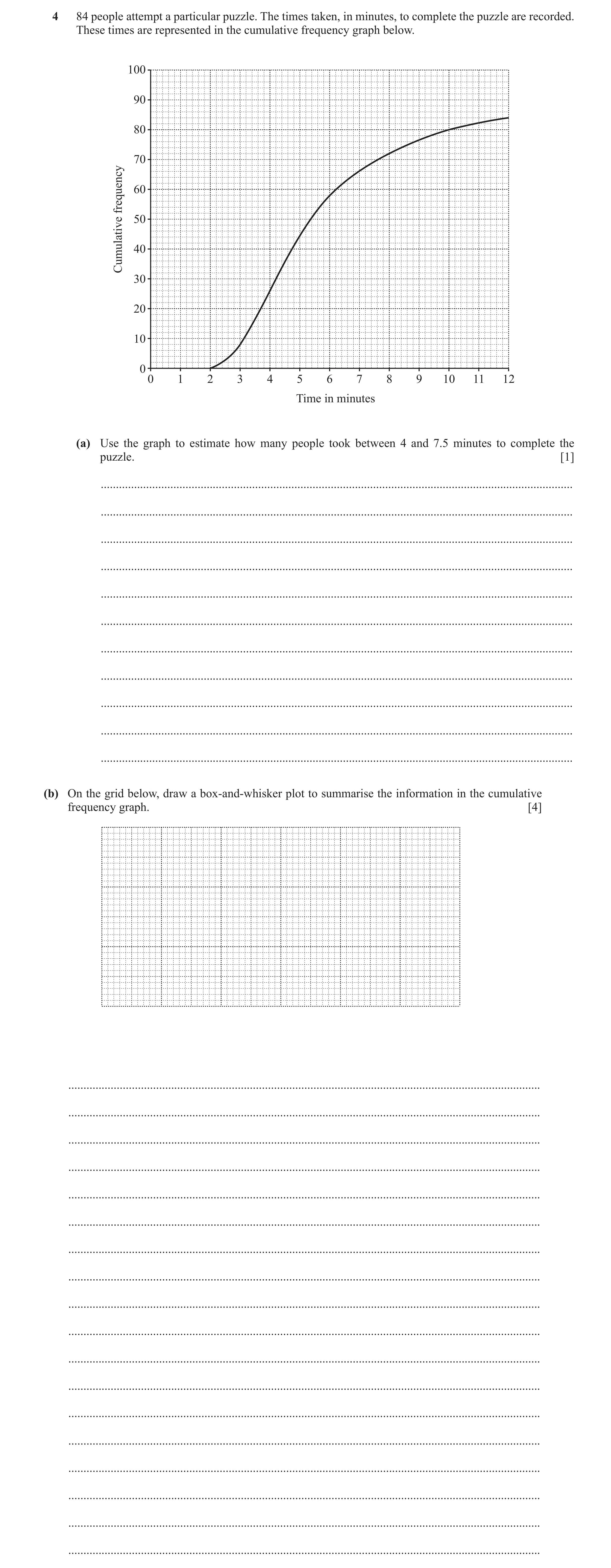
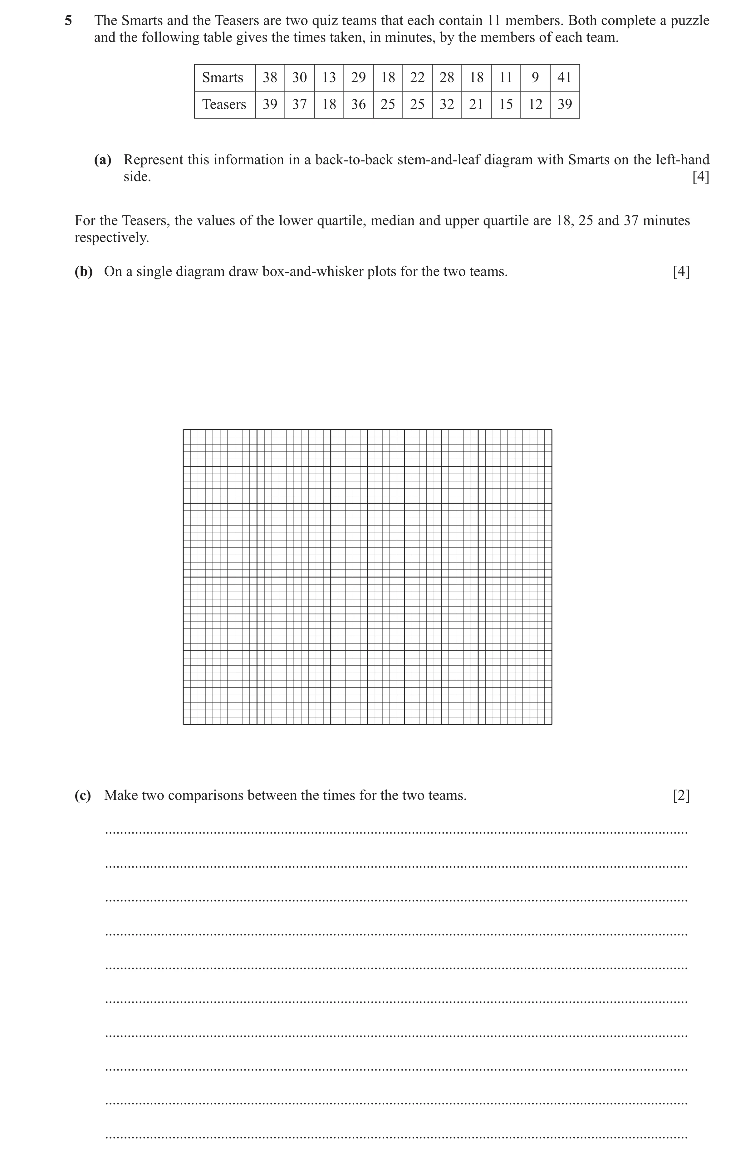
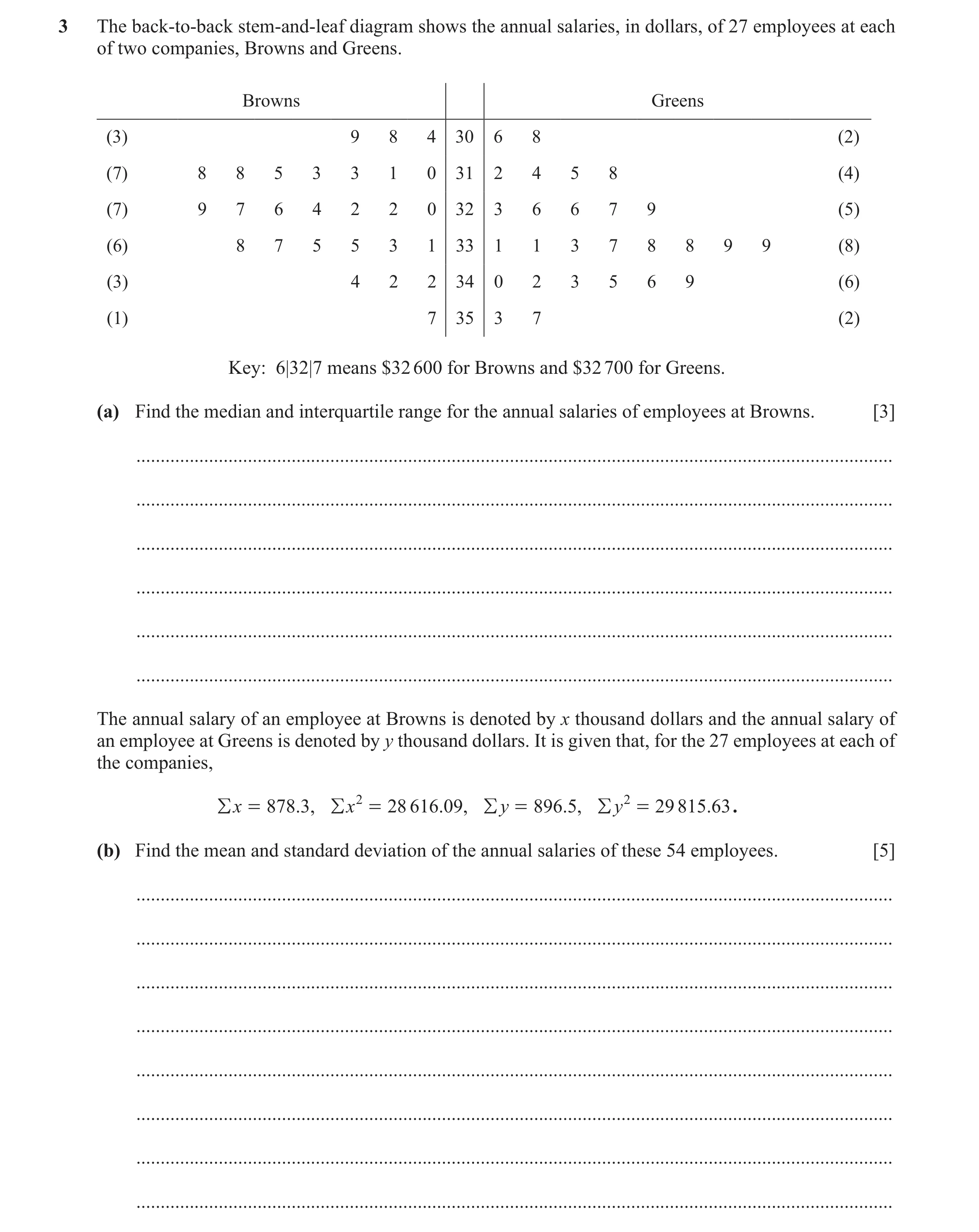 77 / 83
![Question 49: (b) Calculate an estimate of the mean time taken by the 240 competitors. [3] ..............................................................…](https://img.pastlit.com/crops/2871b5ca-95ca-43ec-9f29-64f66bd19dca/q5.webp)
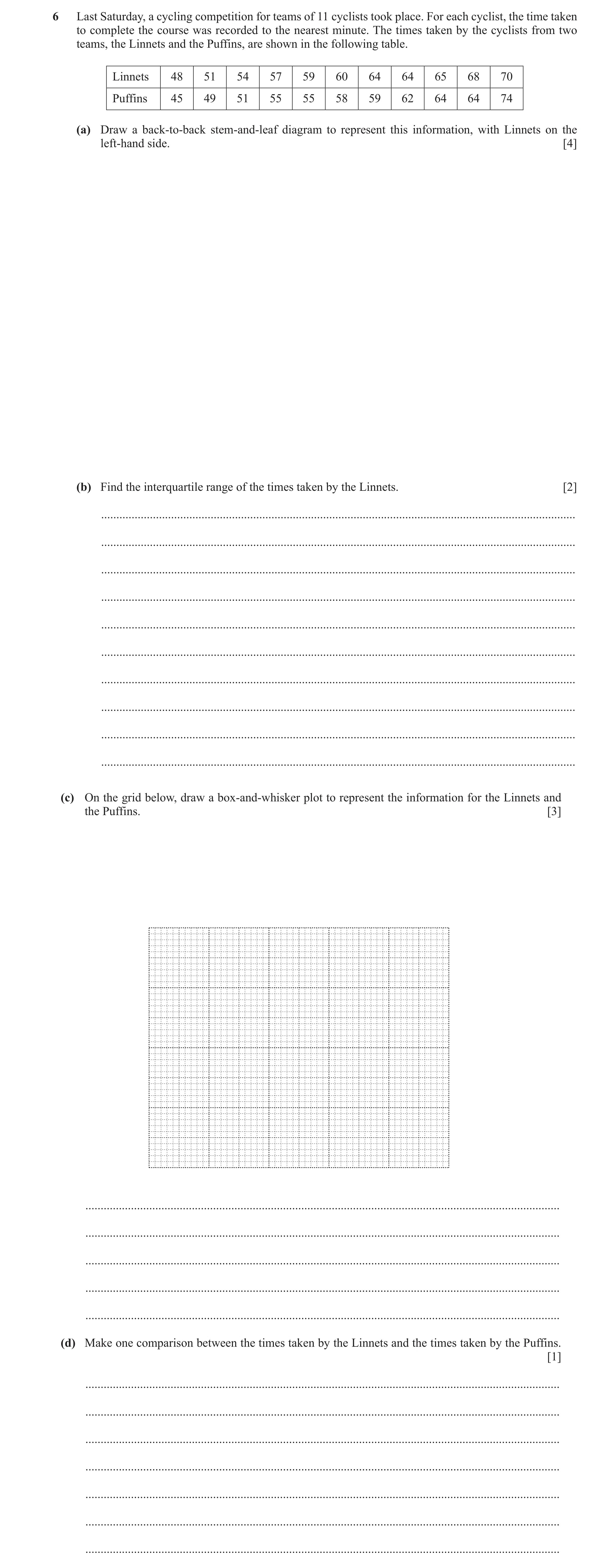
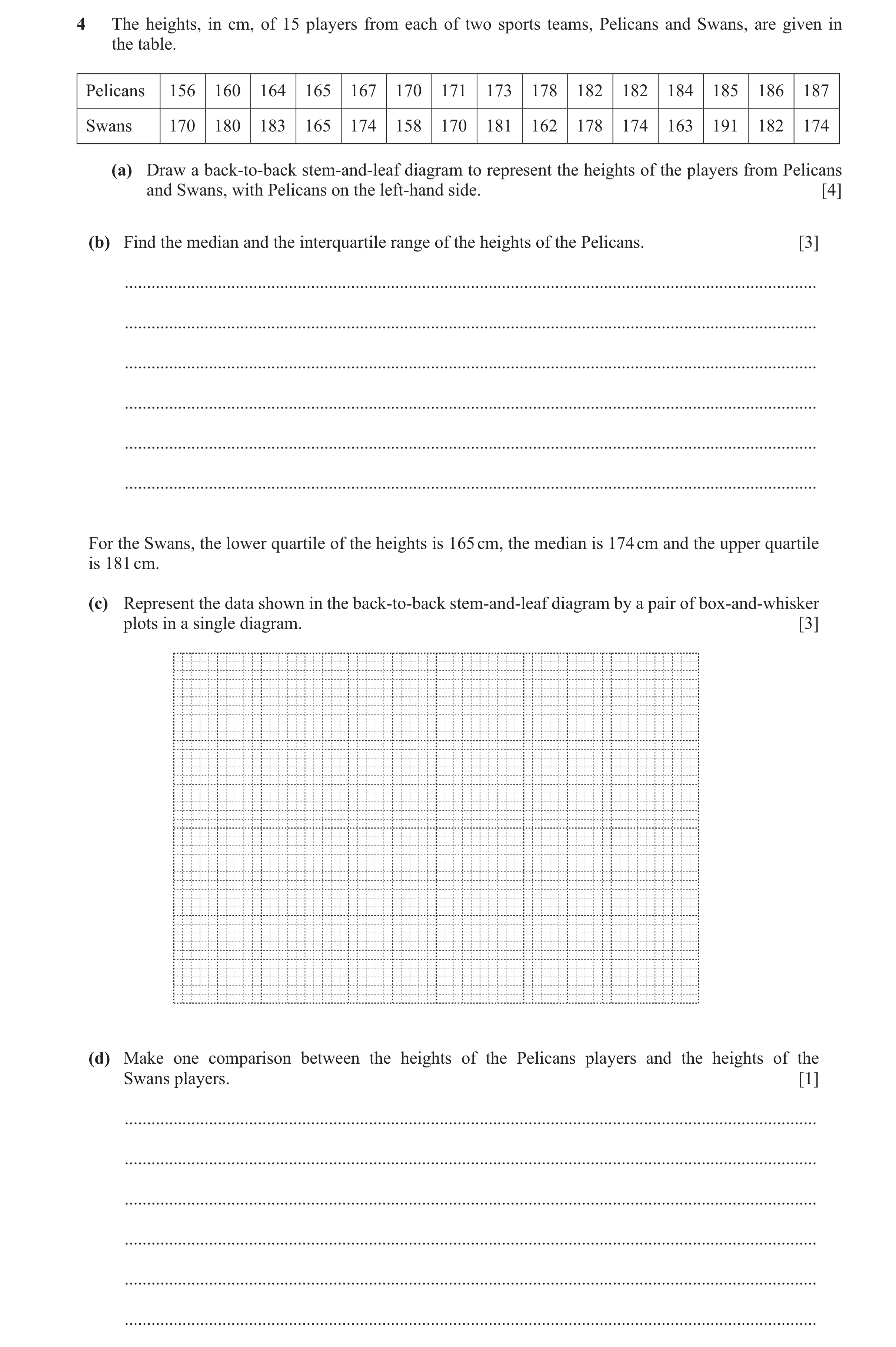
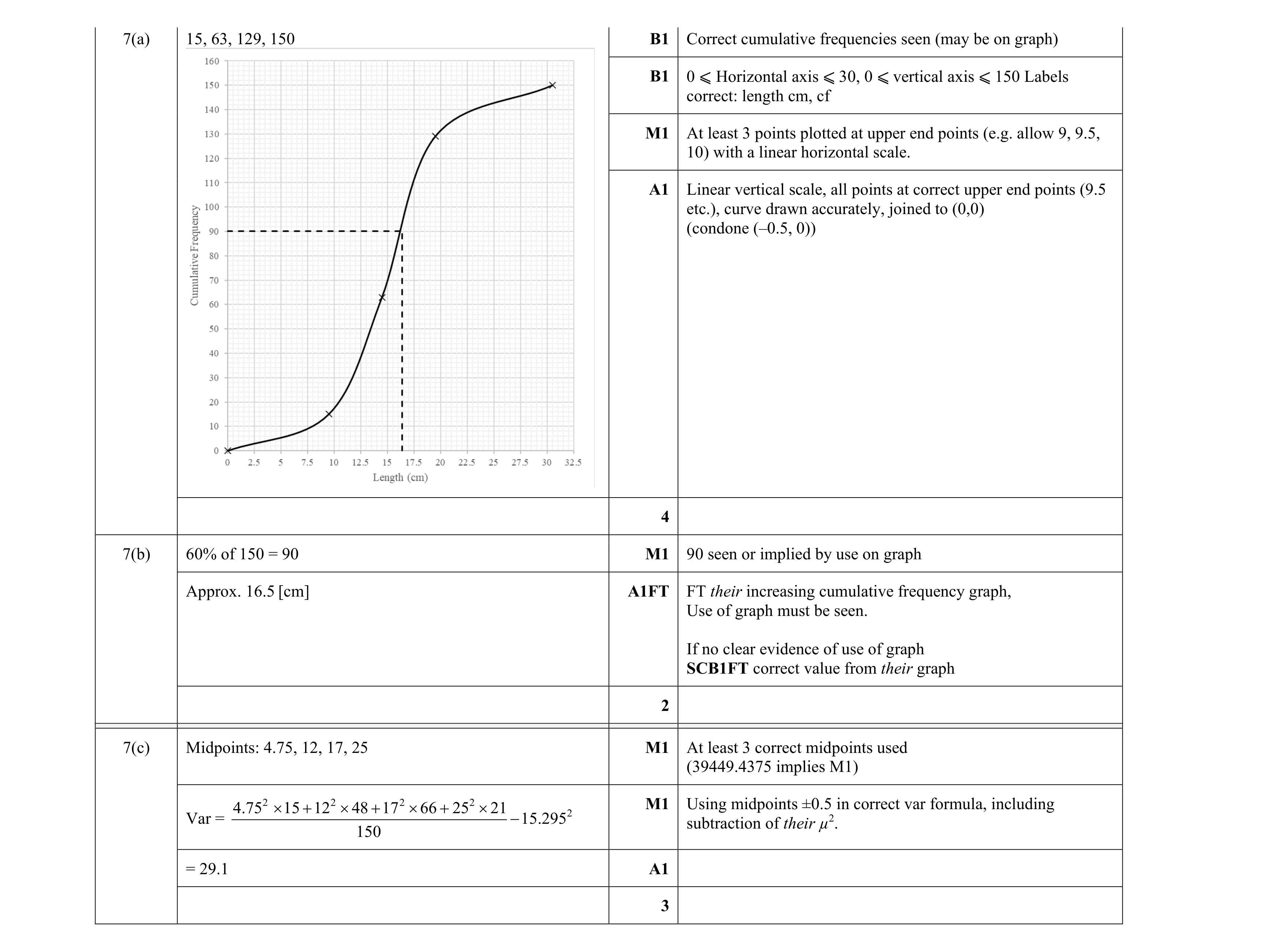 9
9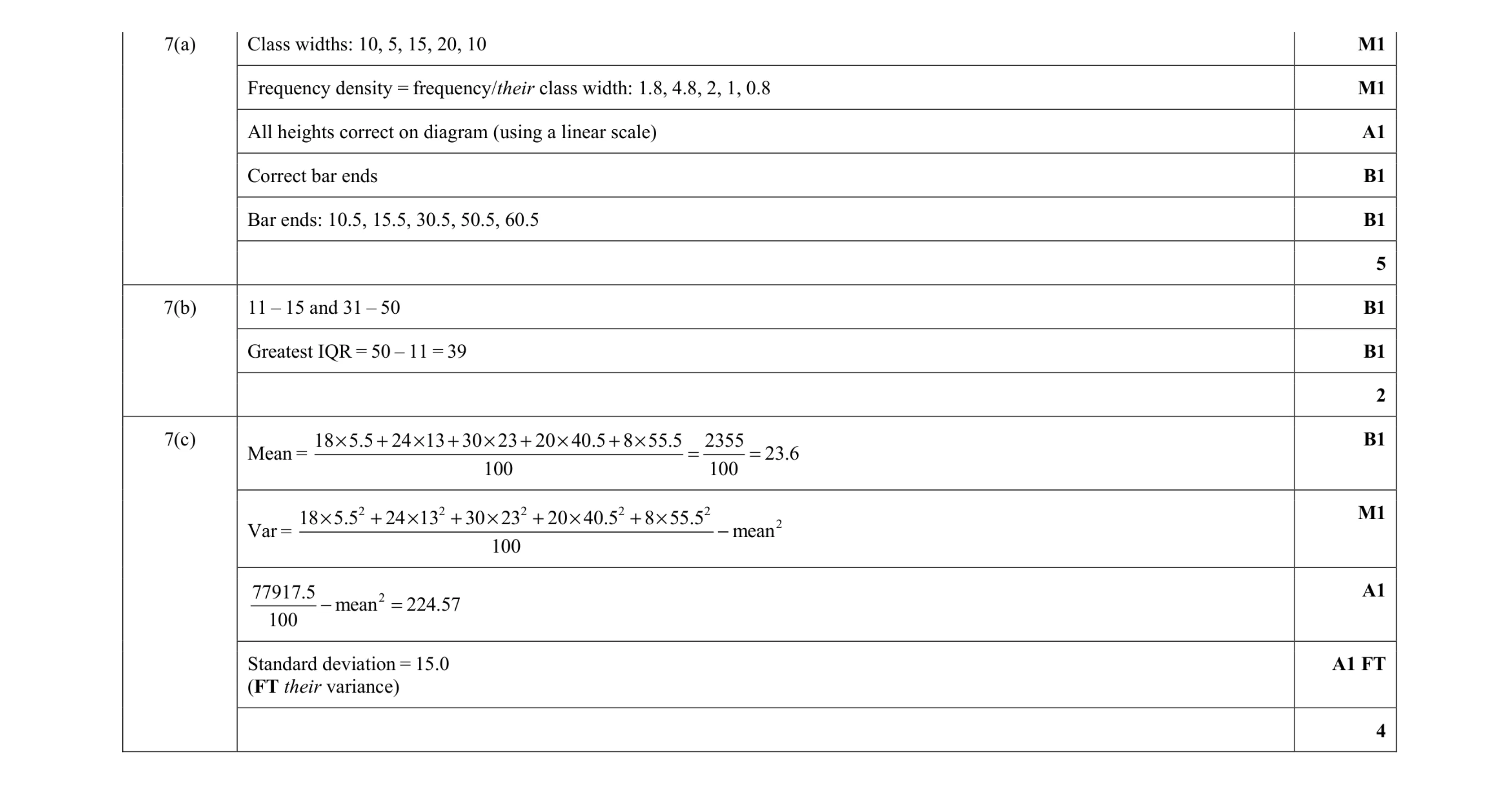 11
11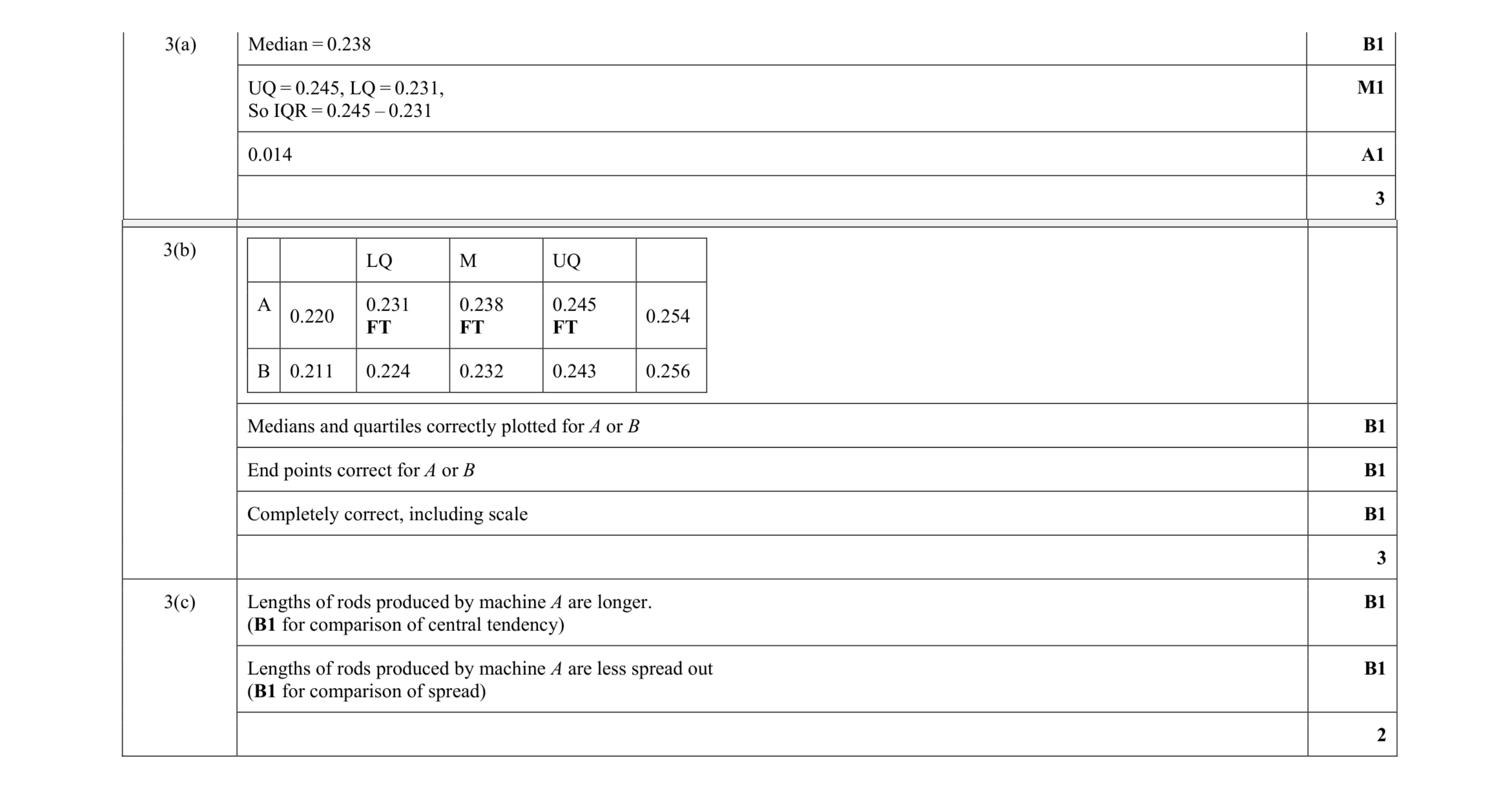 8
8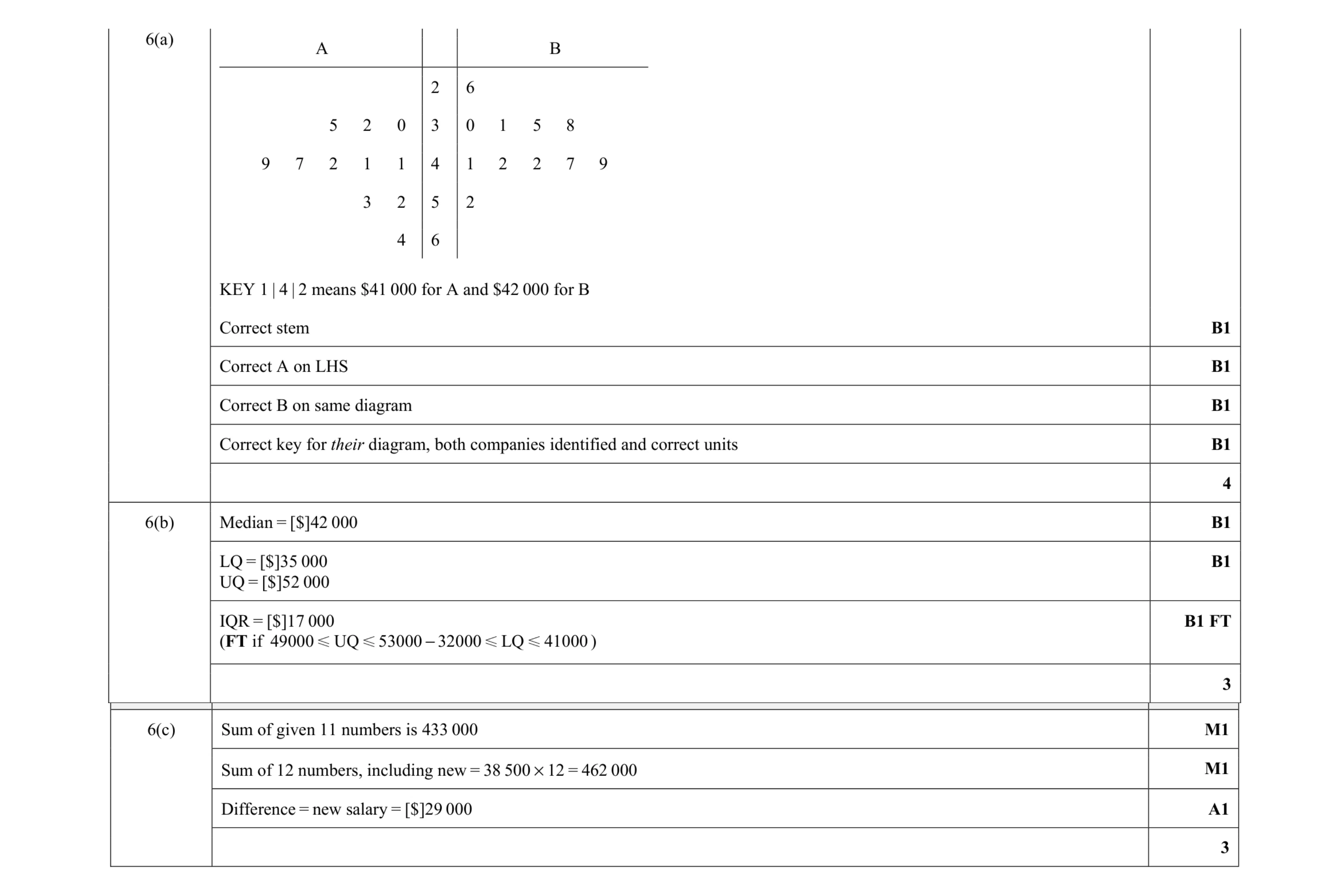 10
10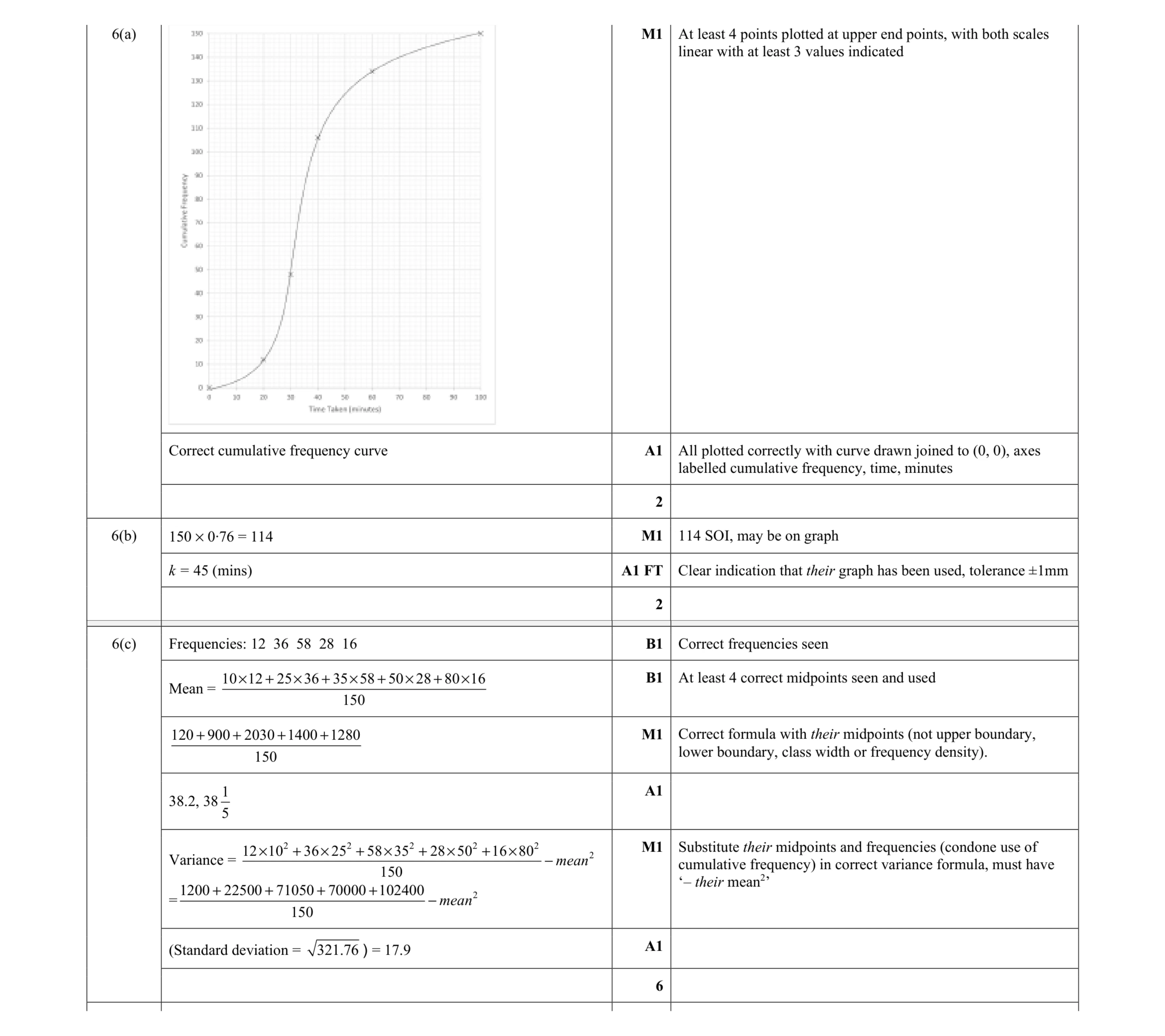 10
10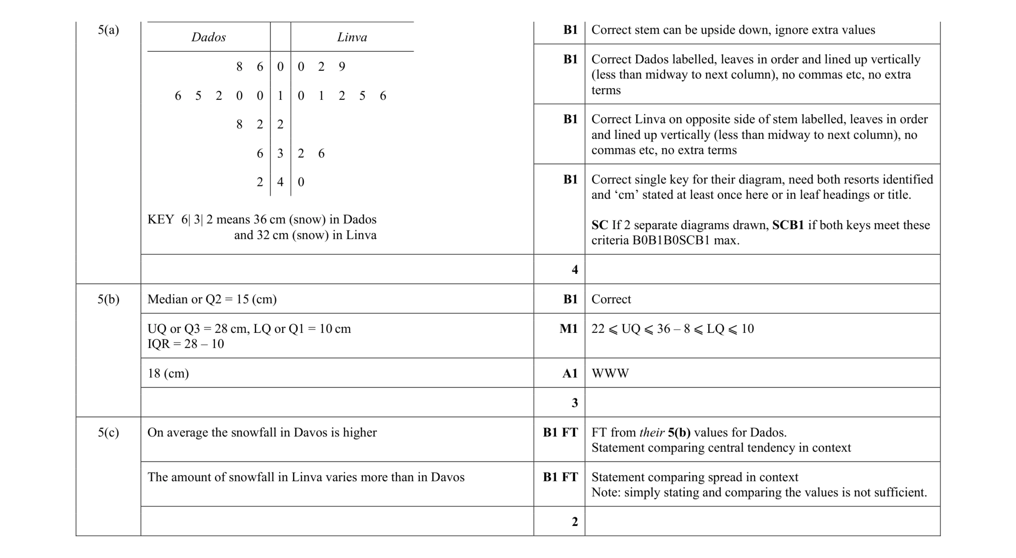 9
9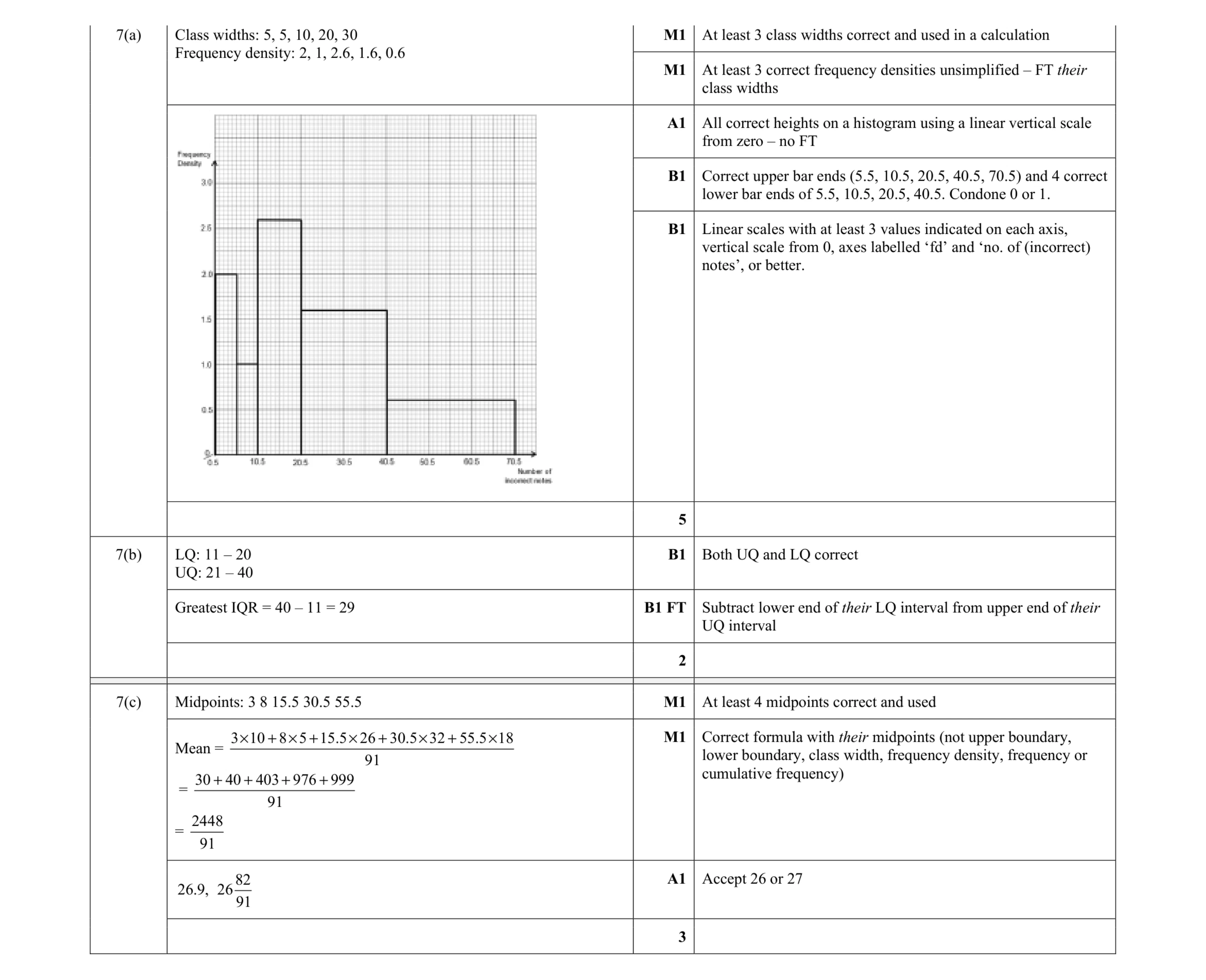 10
10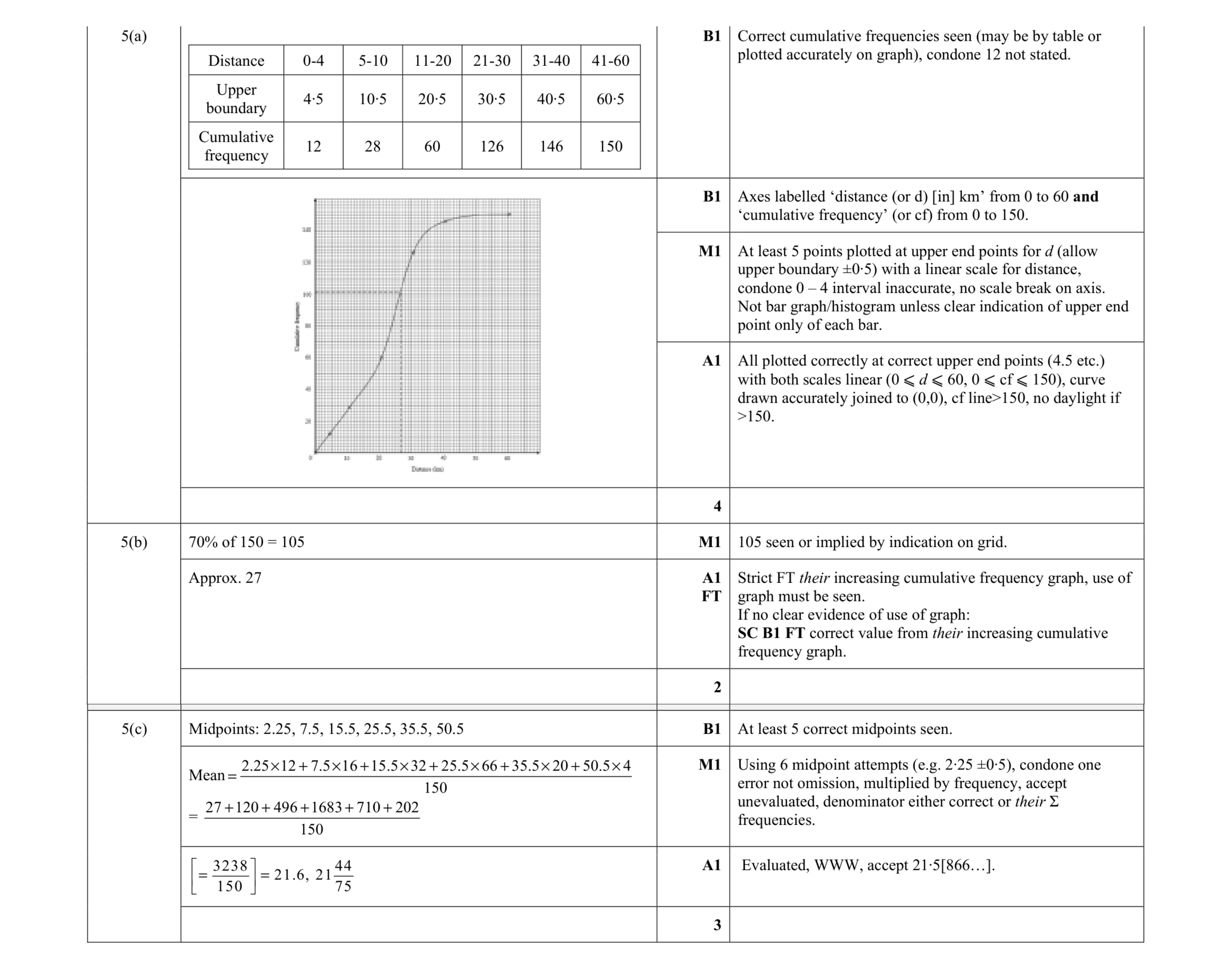 9
9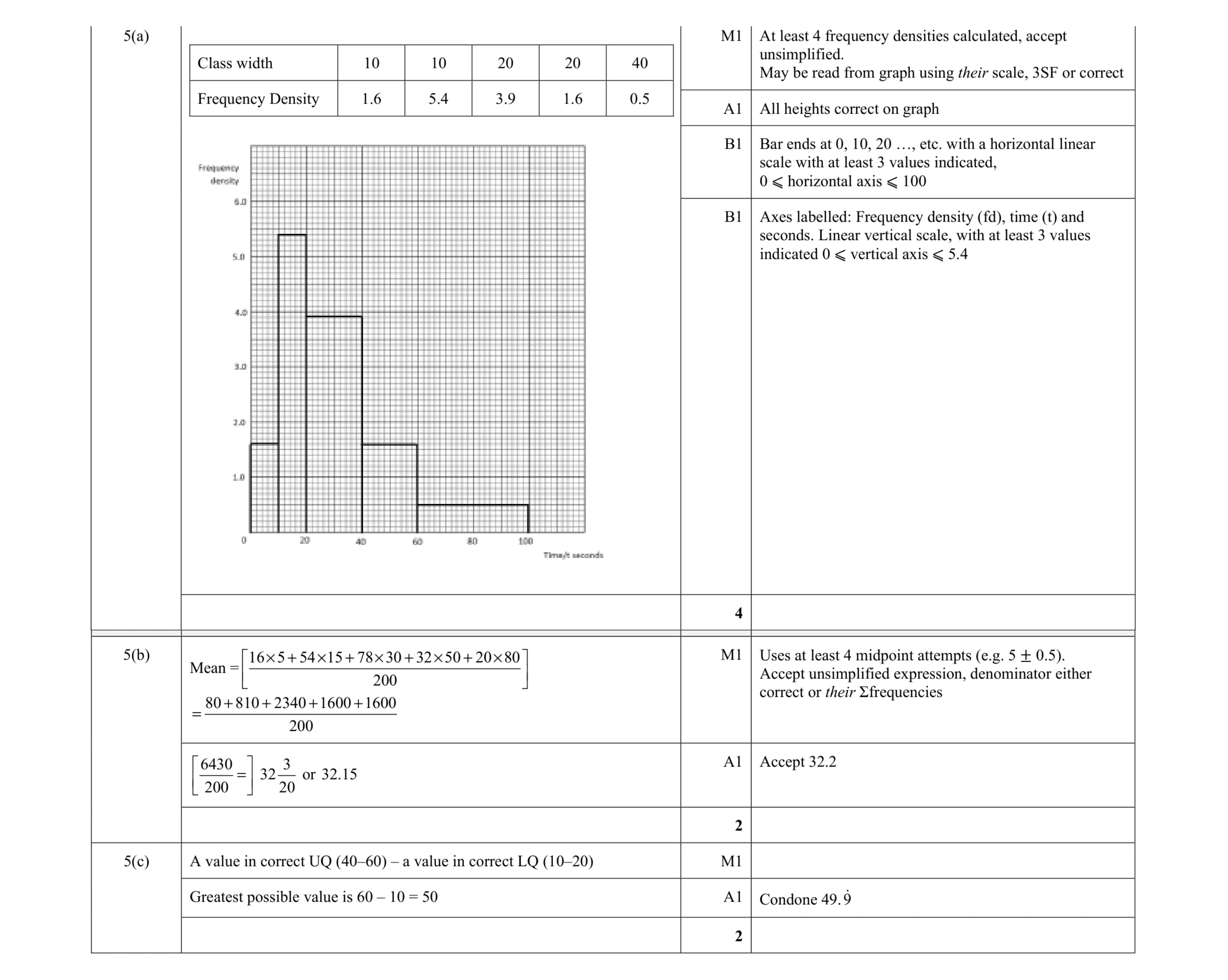 8
8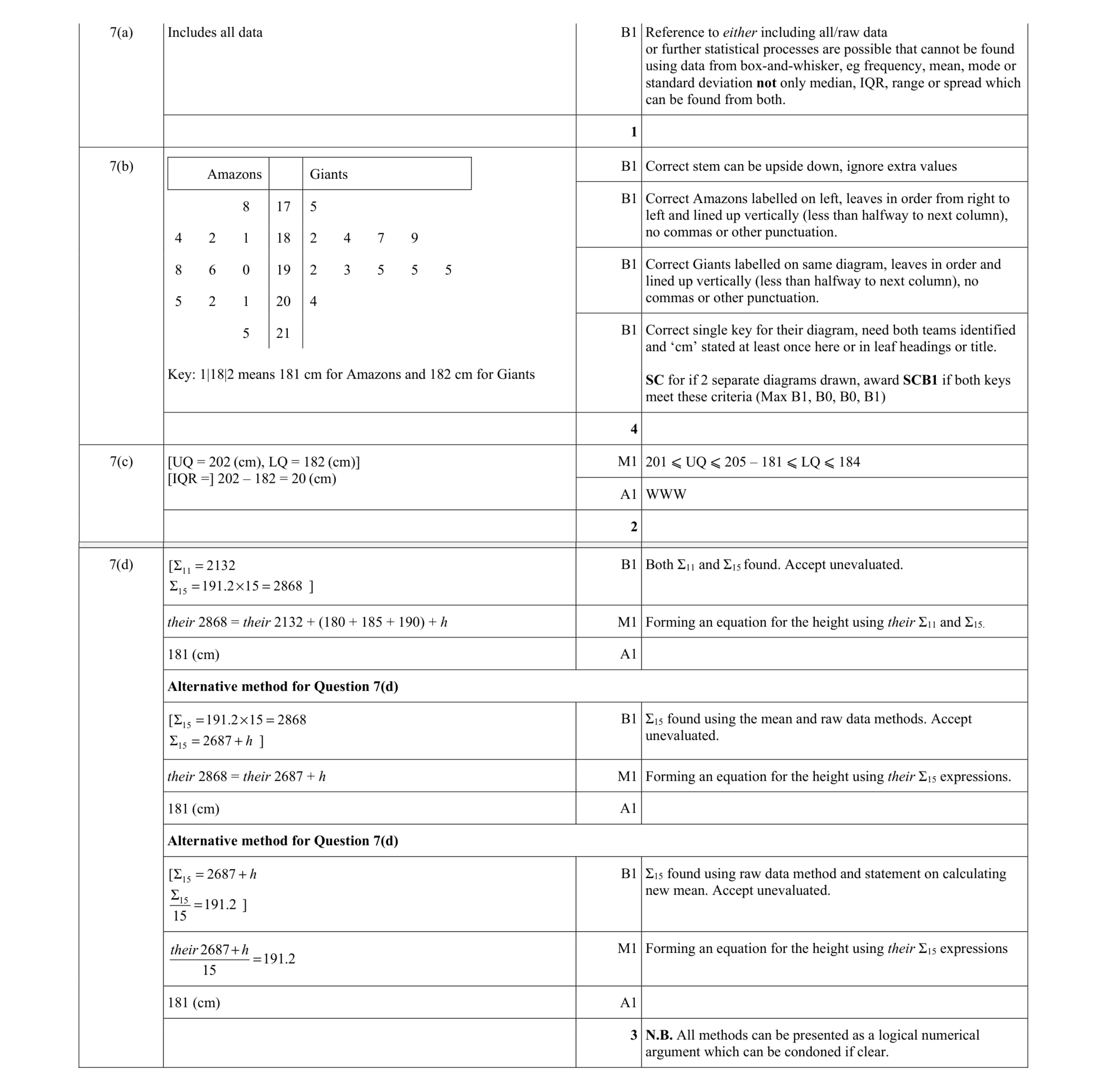 10
10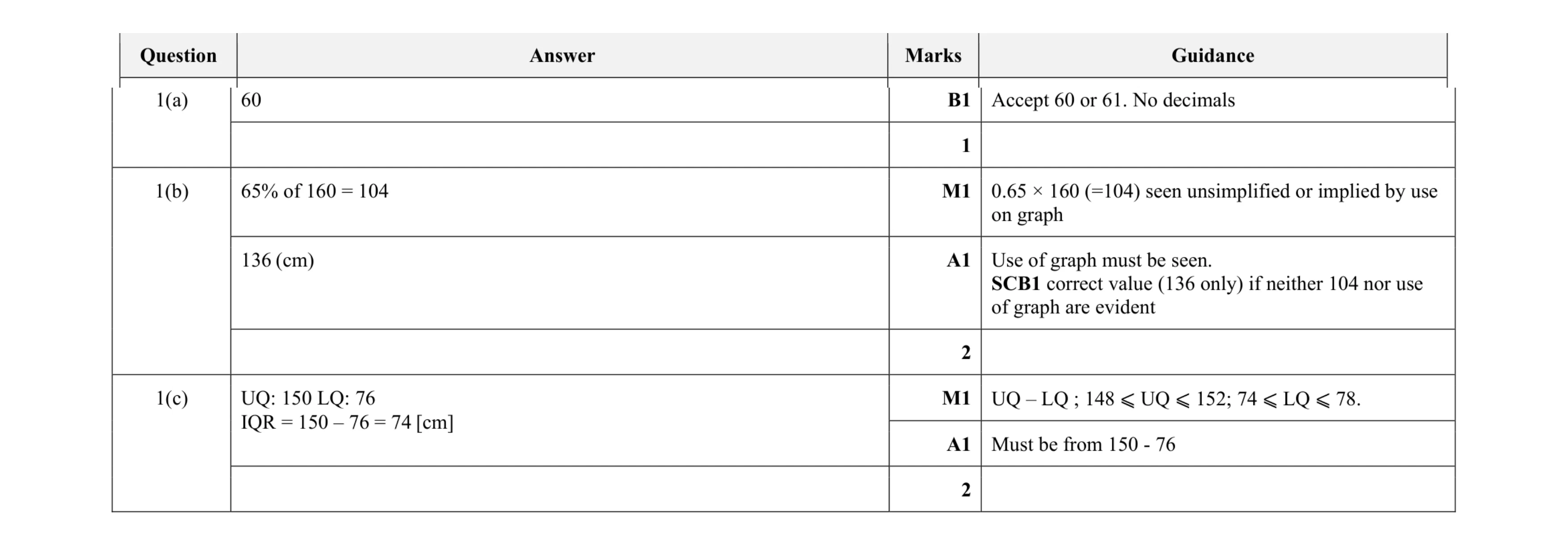 5
5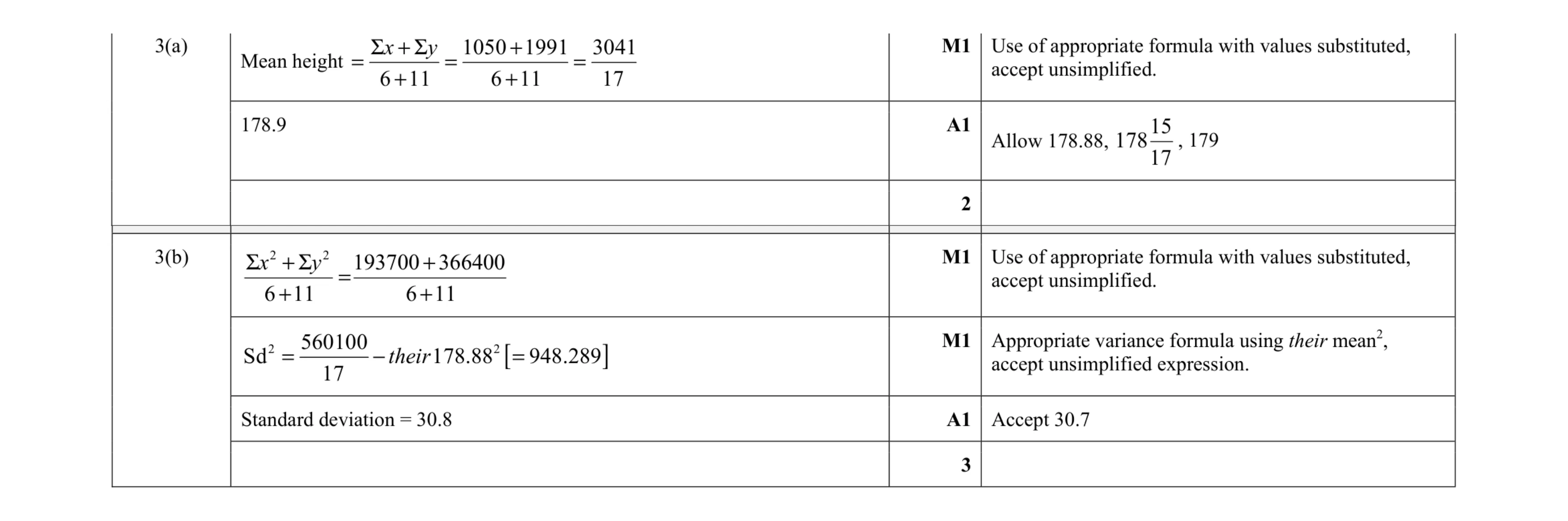 5
5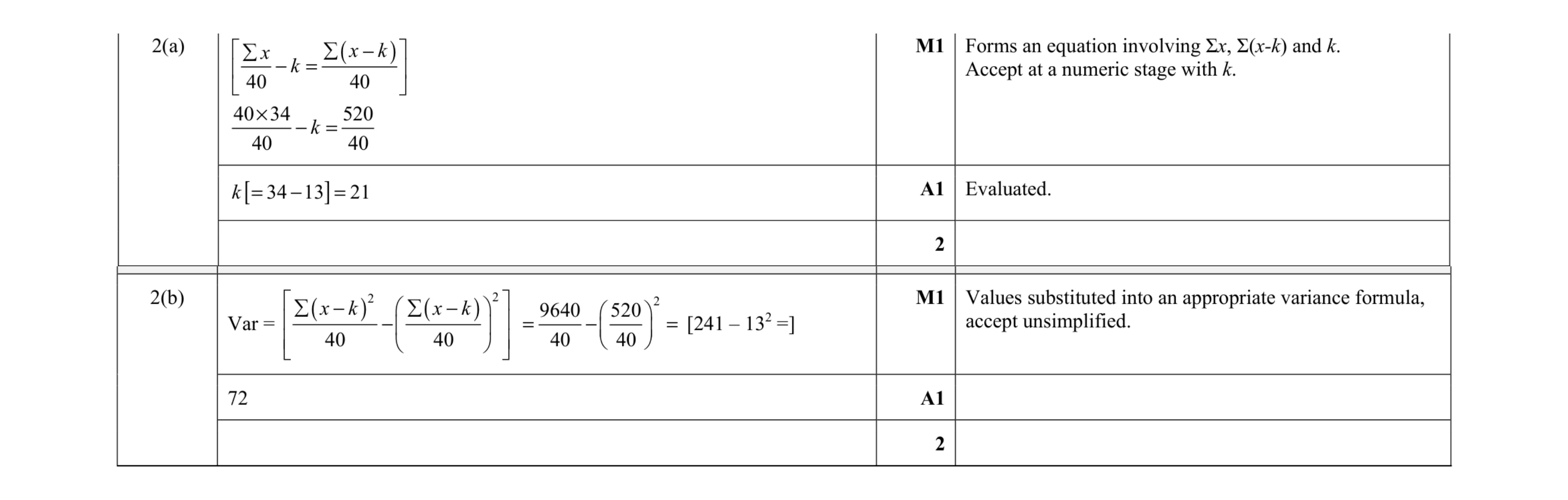 4
4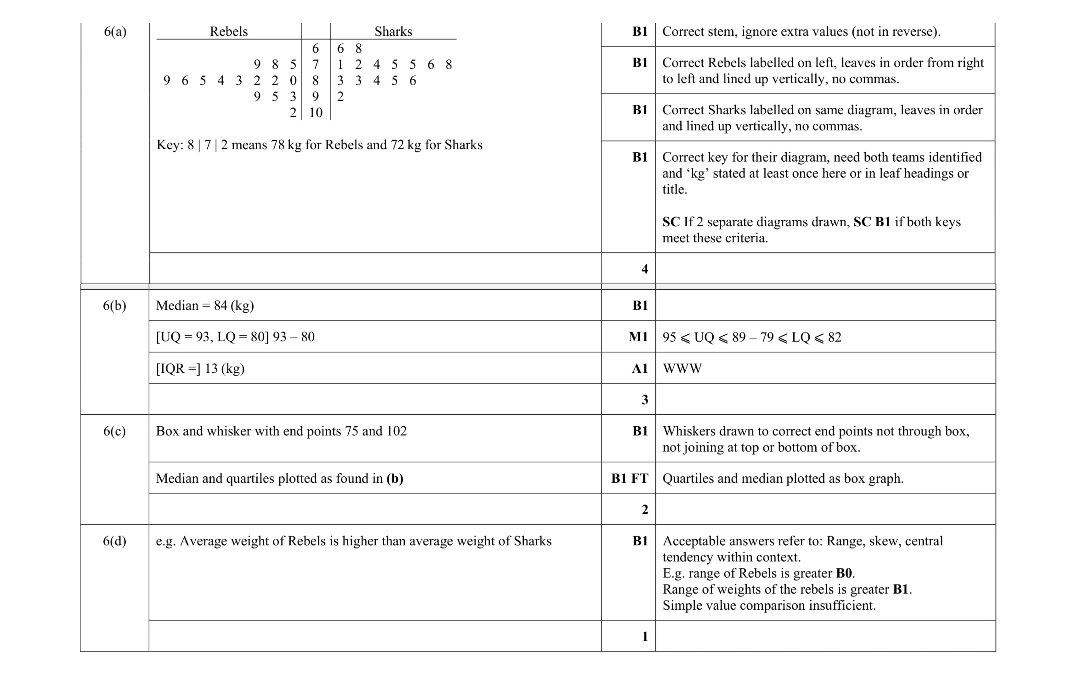 10
10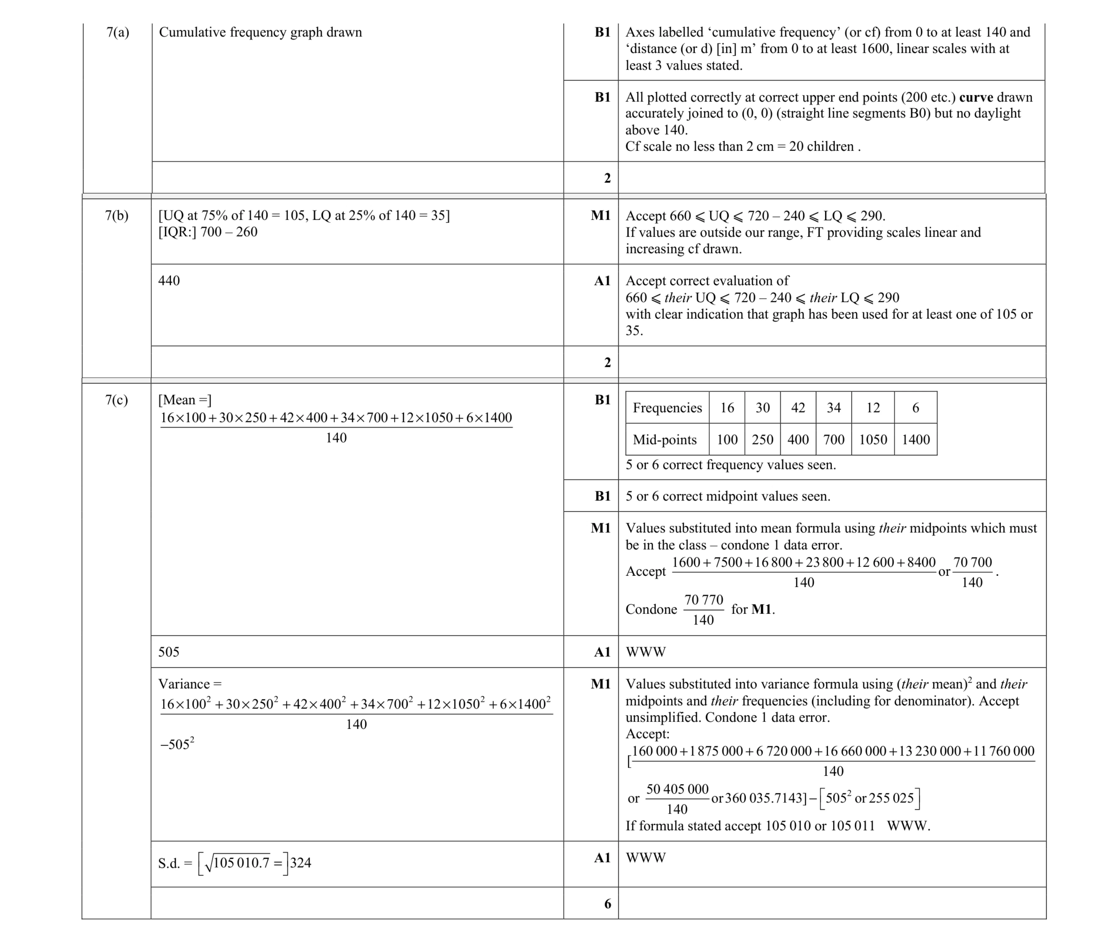 10
10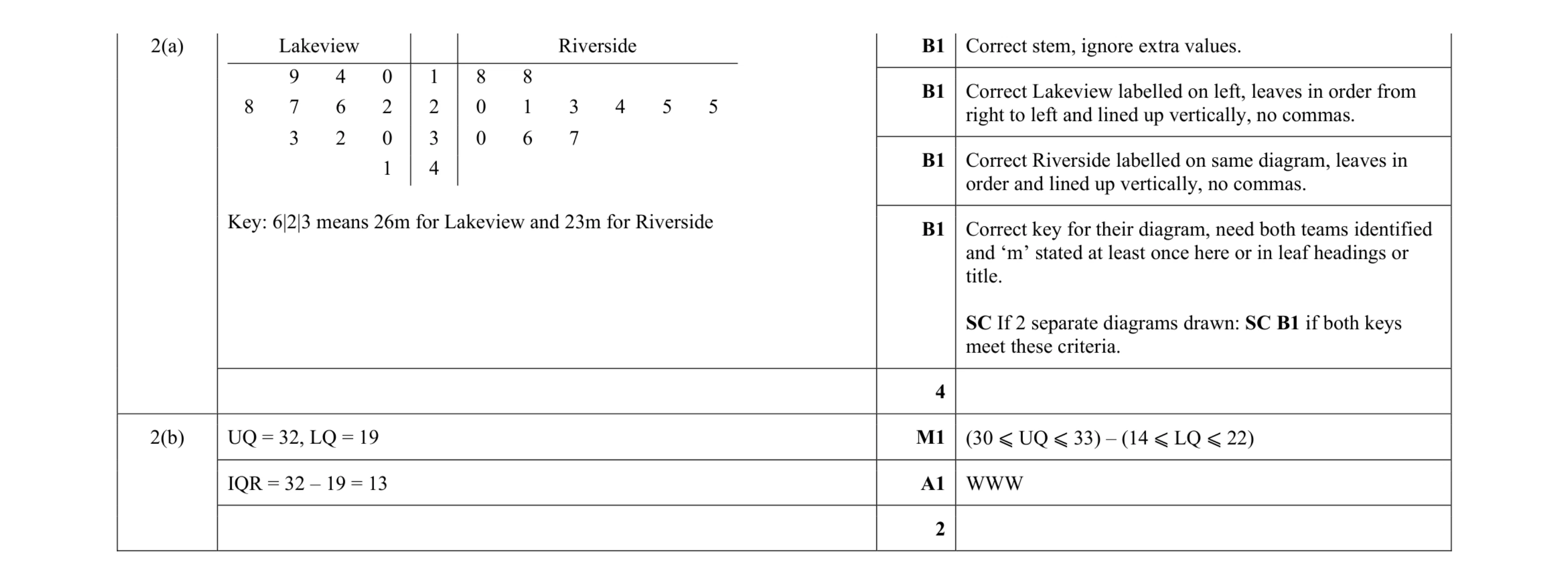 6
6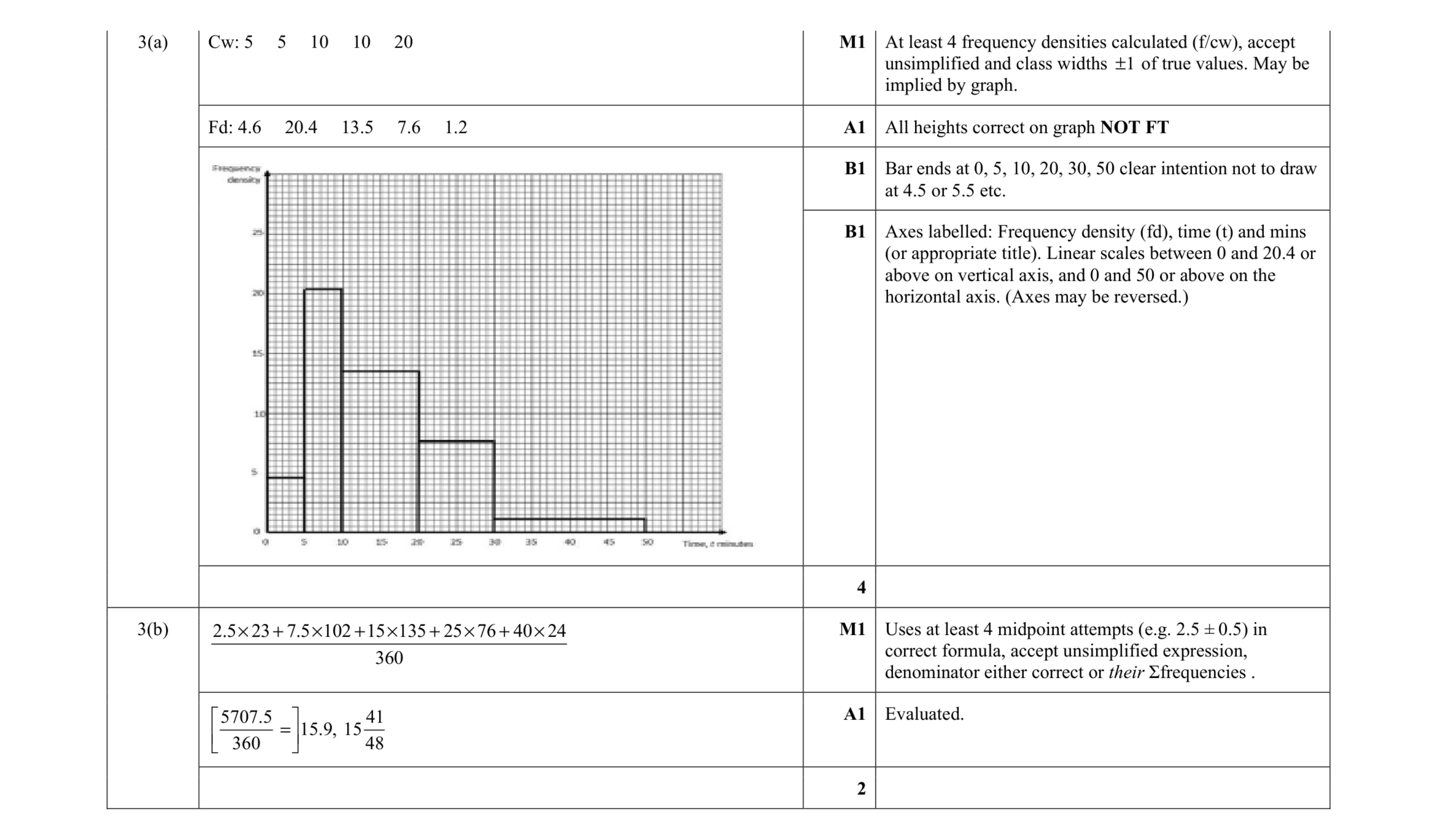 6
6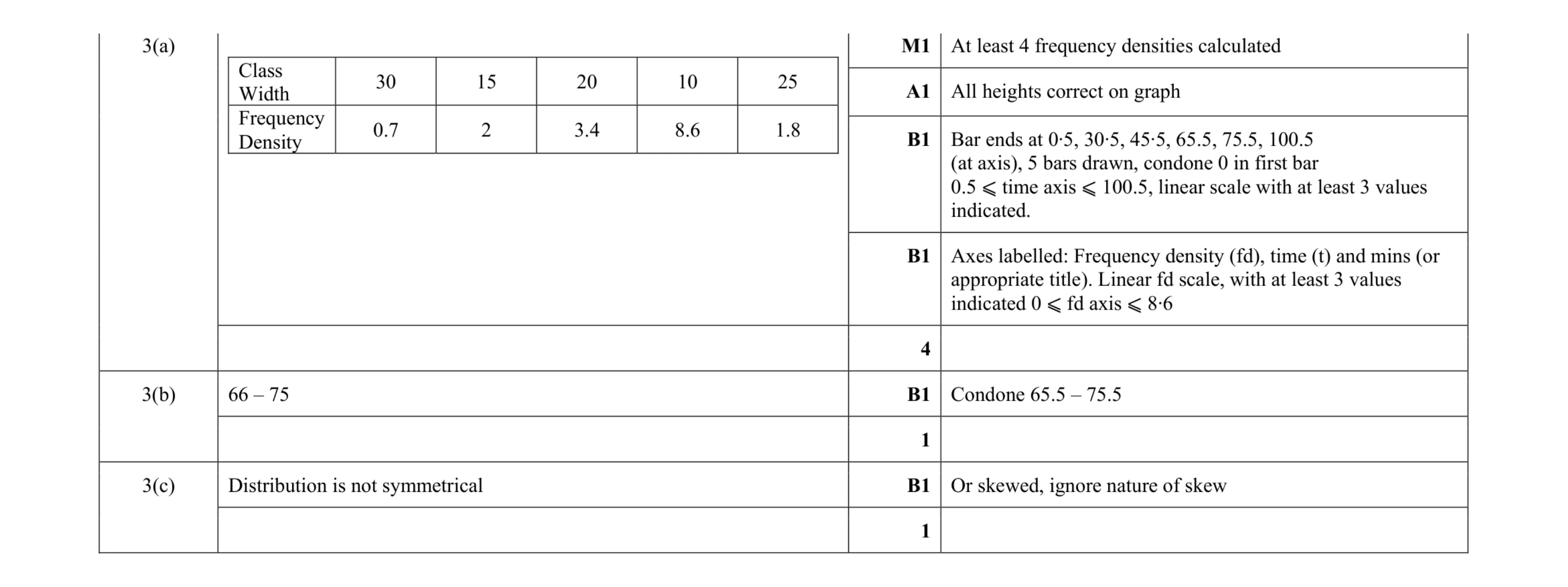 6
6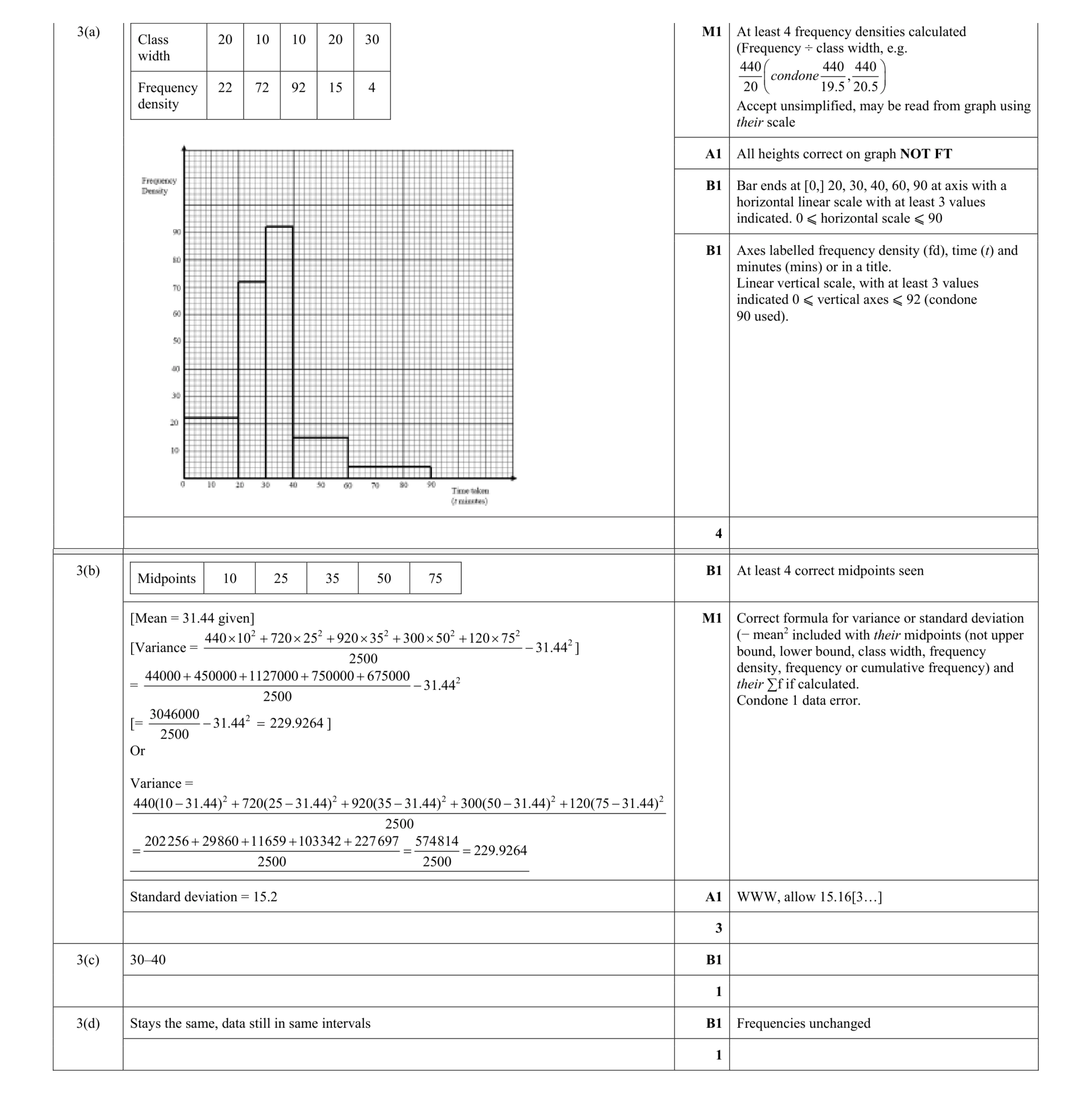 9
9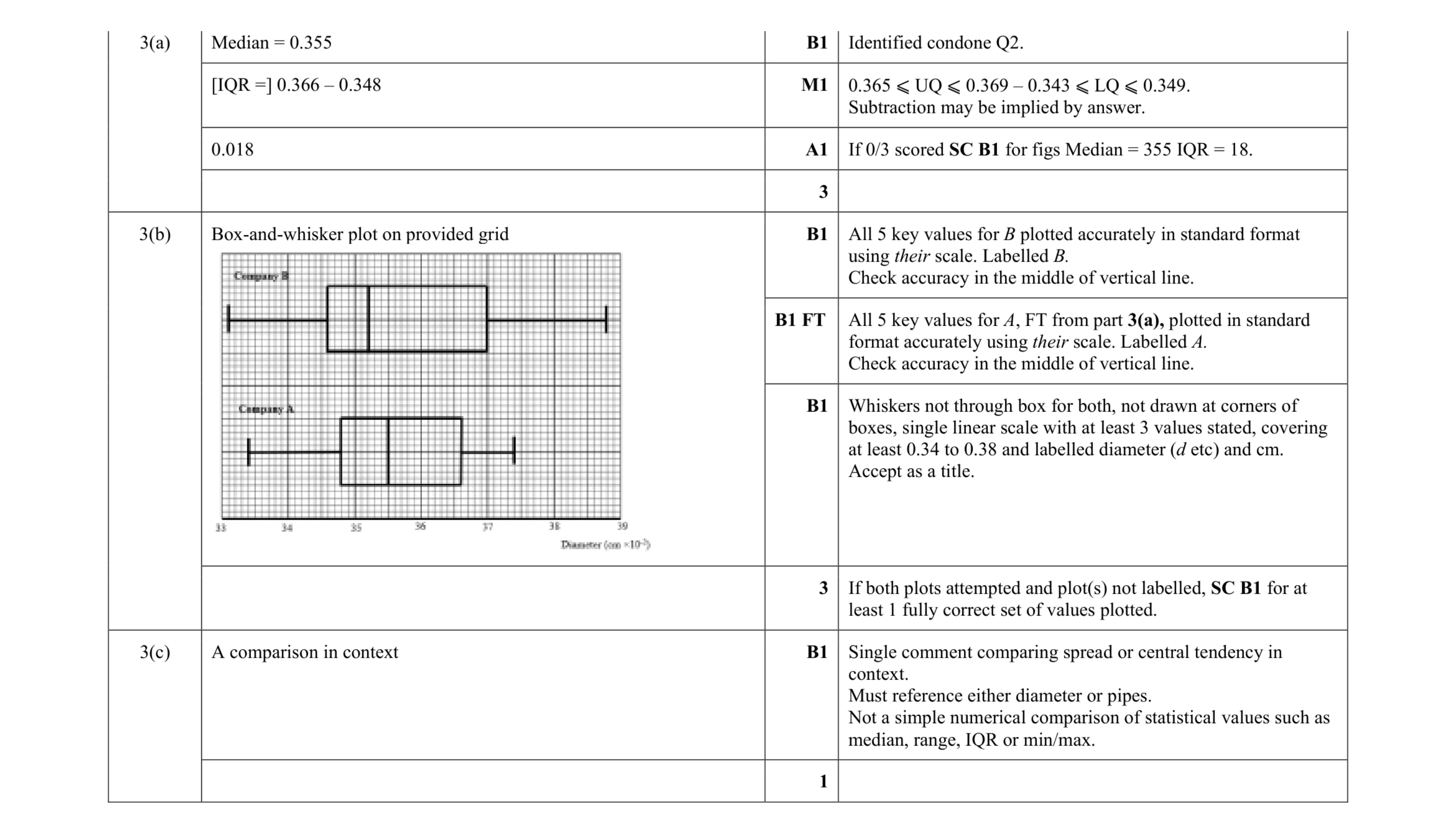 7
7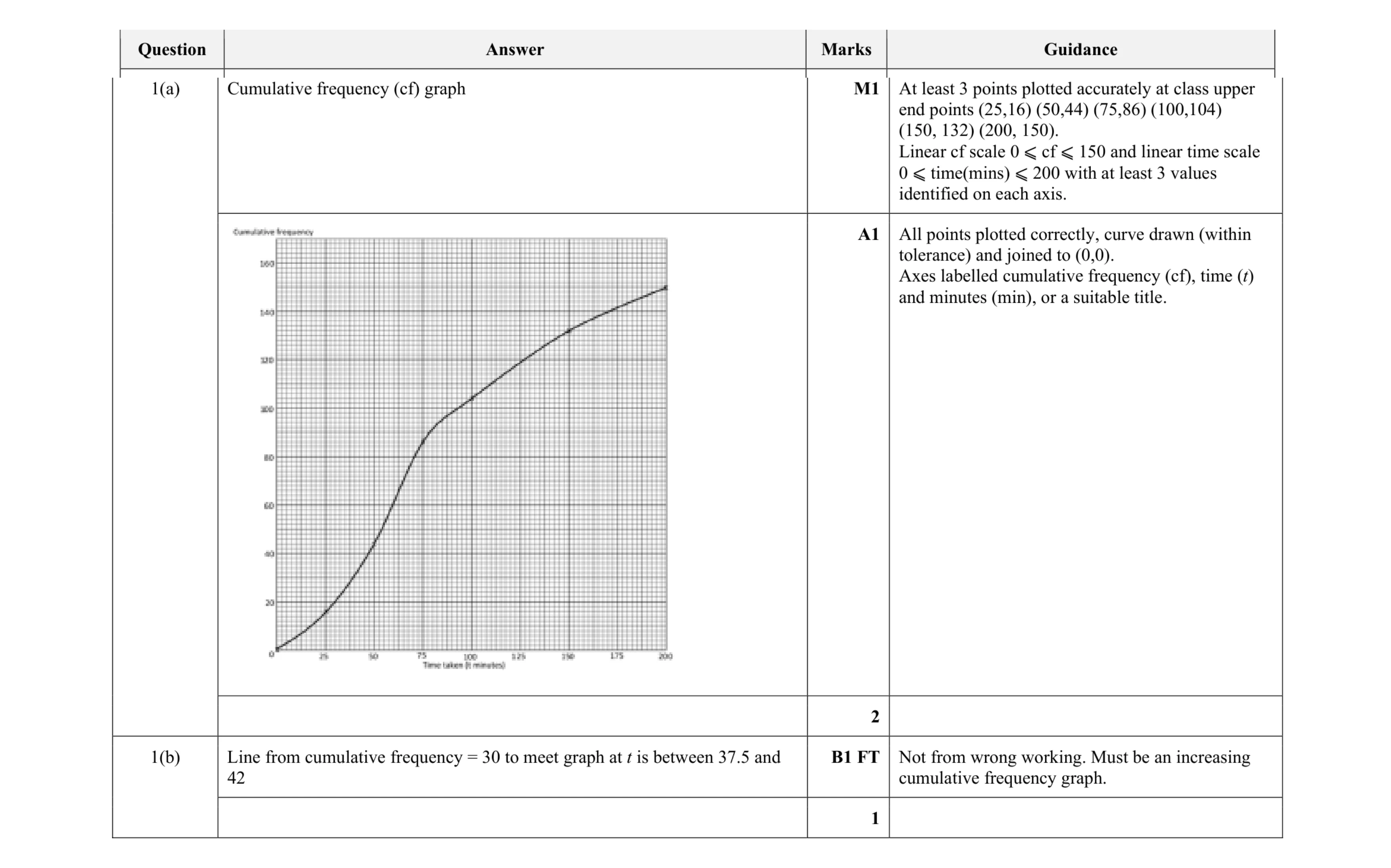 3
3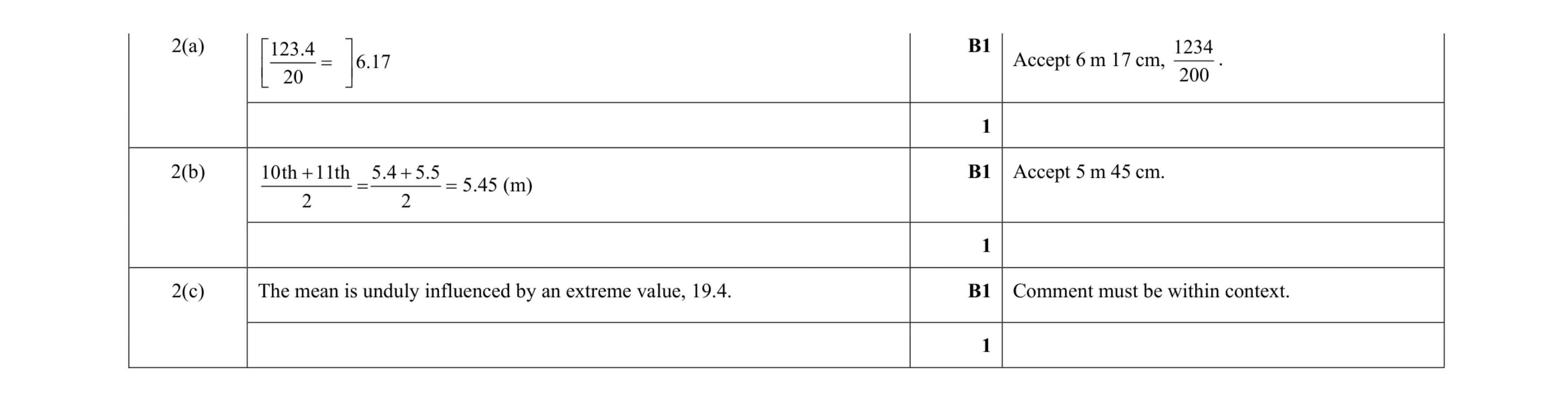 3
3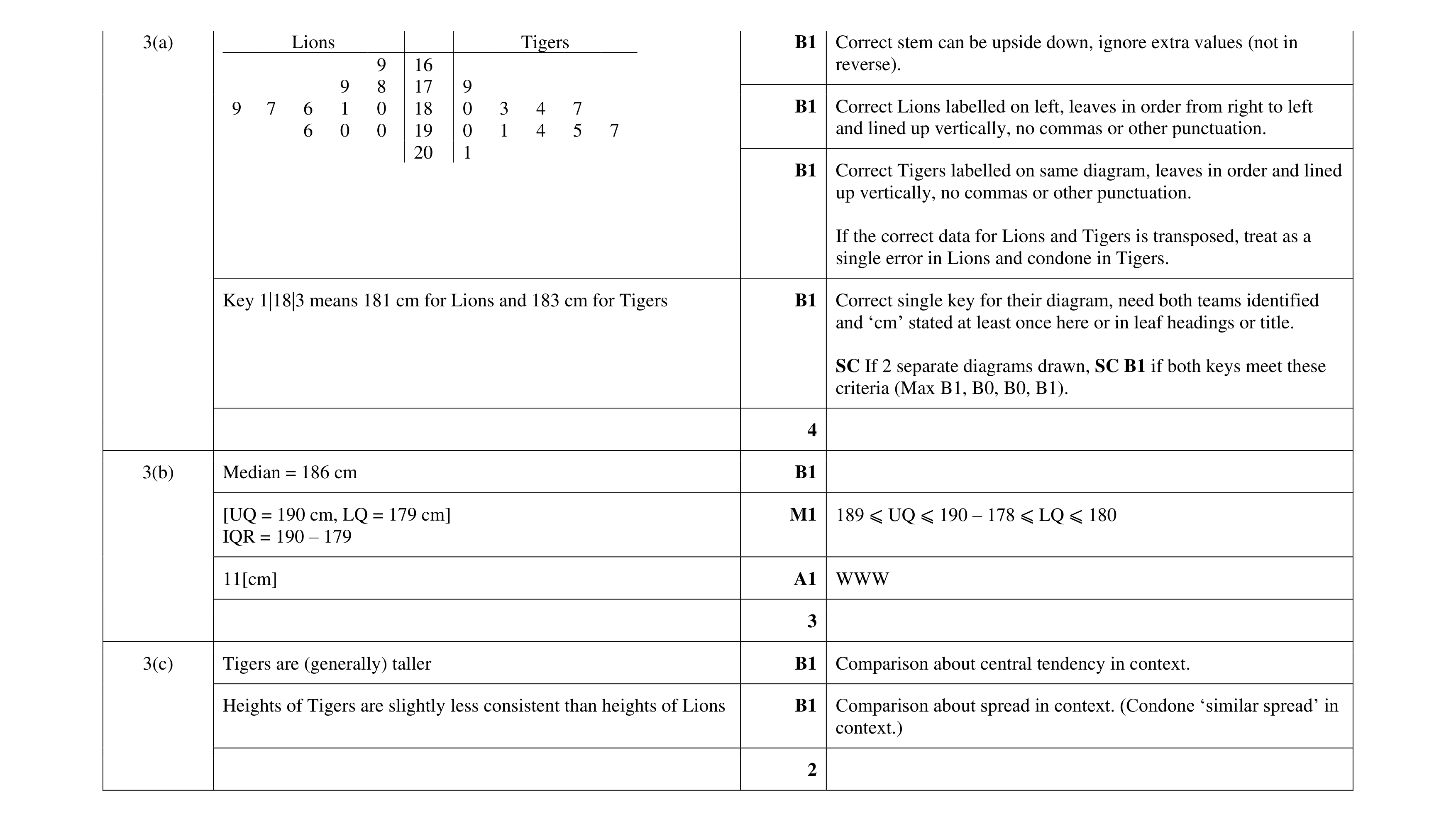 9
9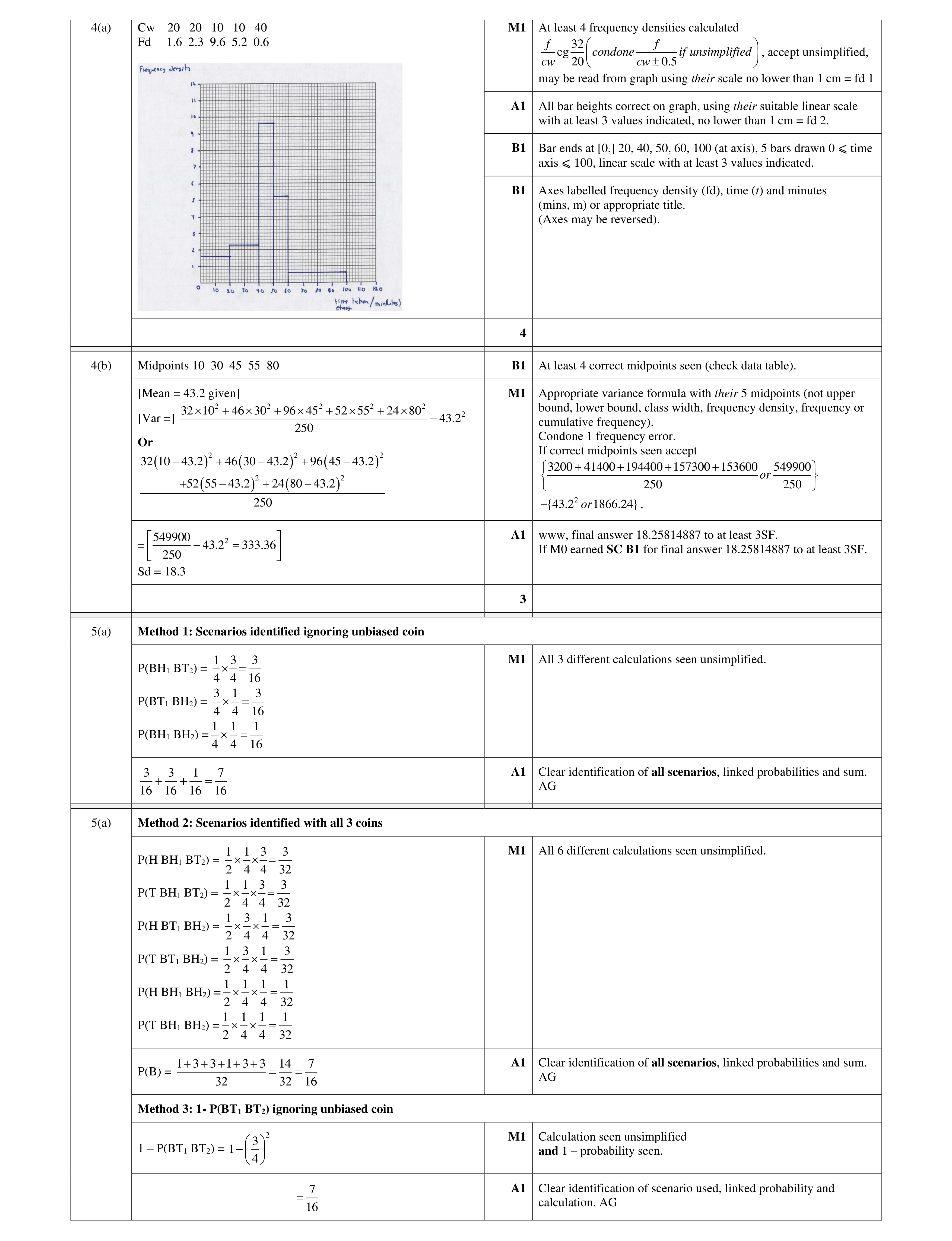 7
7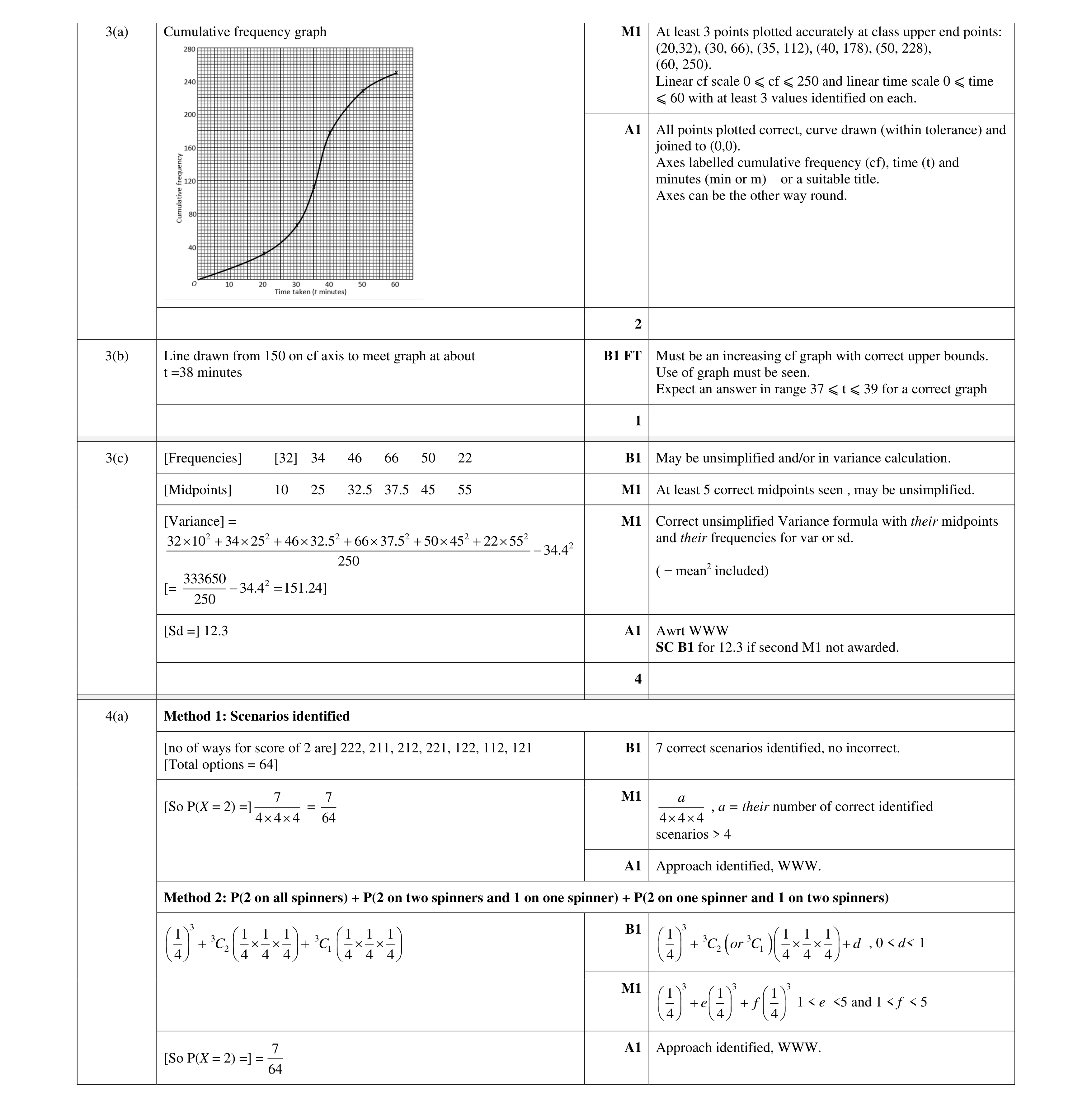 7
7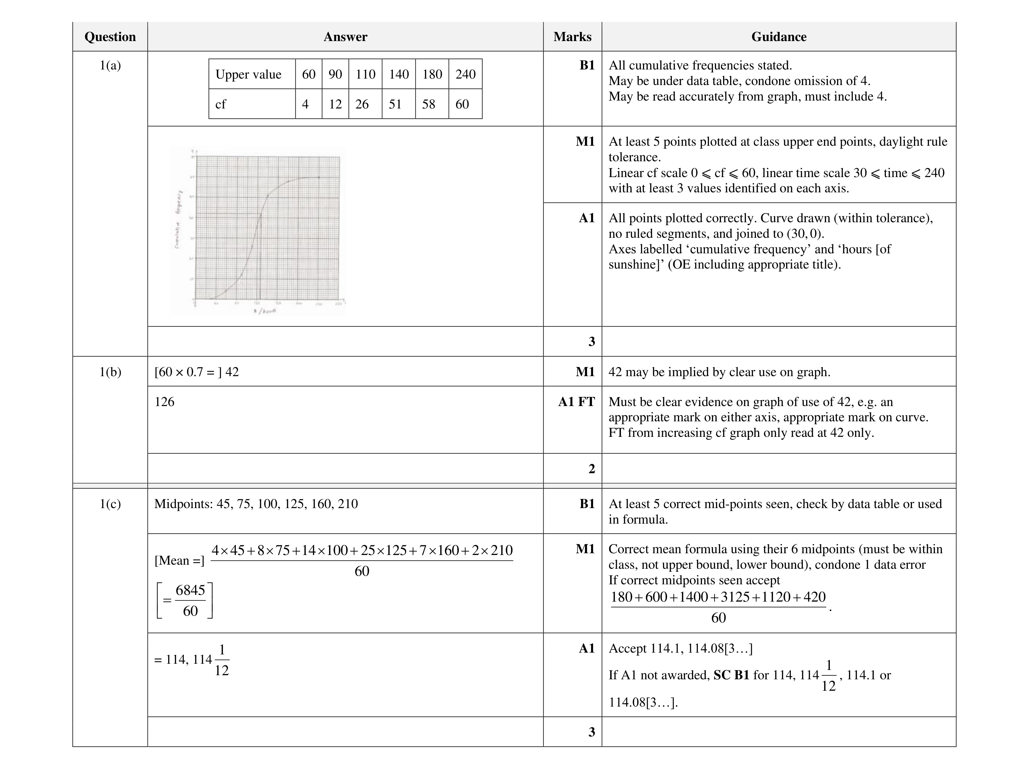 8
8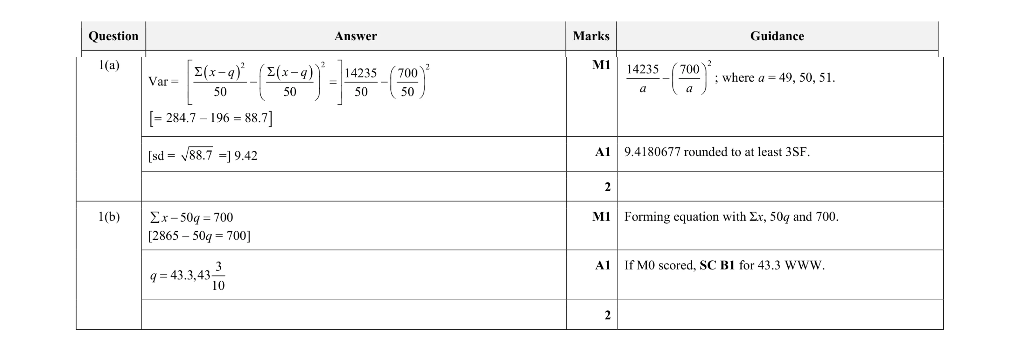 4
4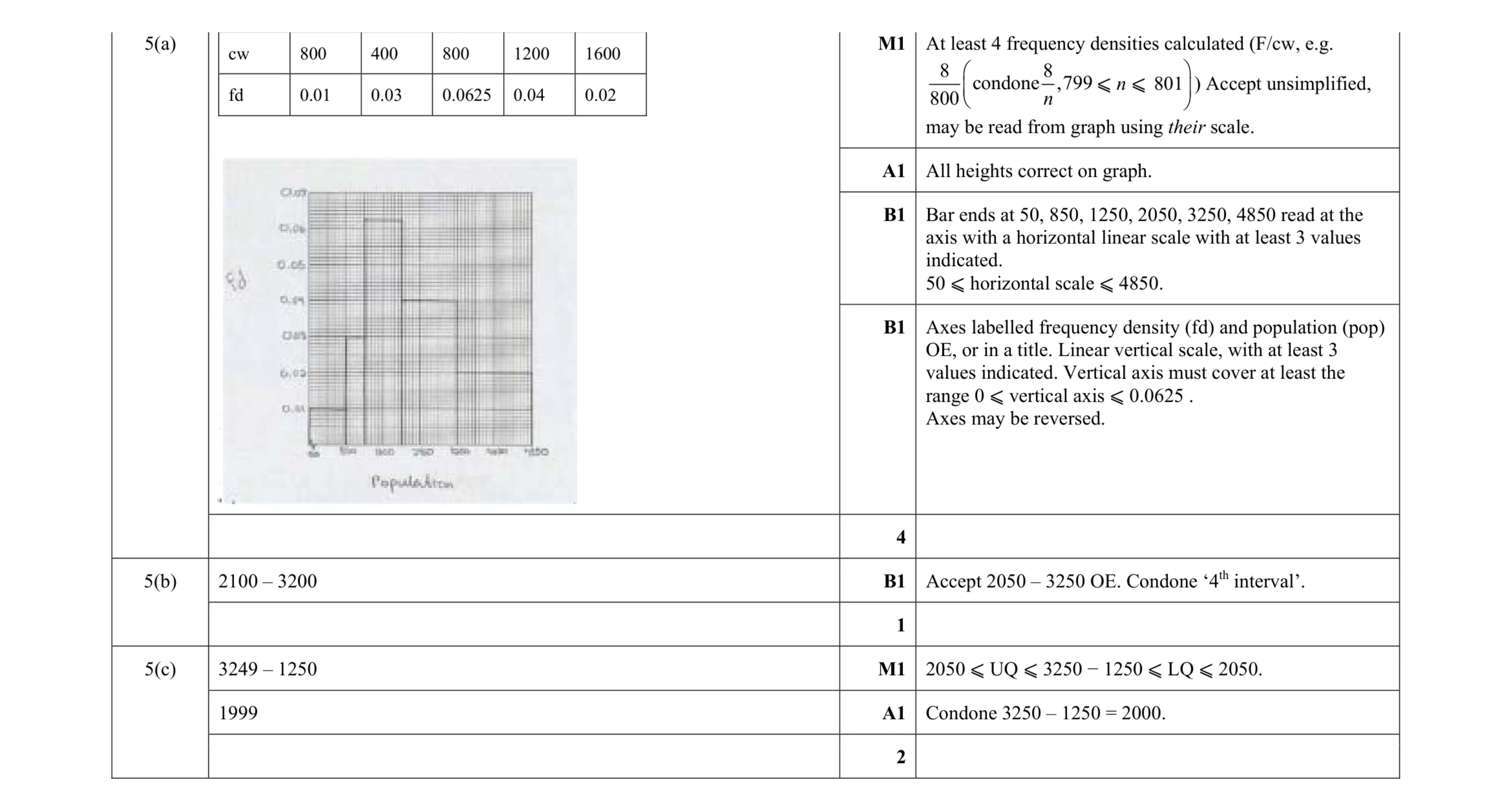 7
7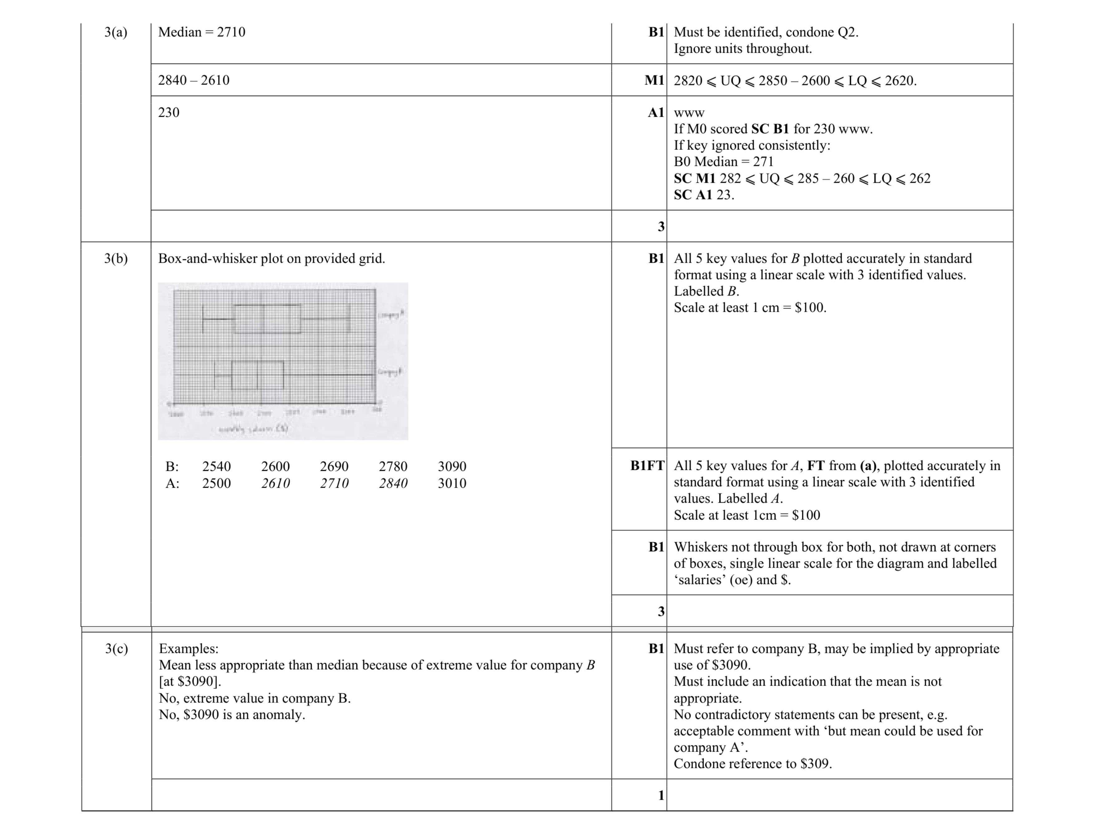 7
7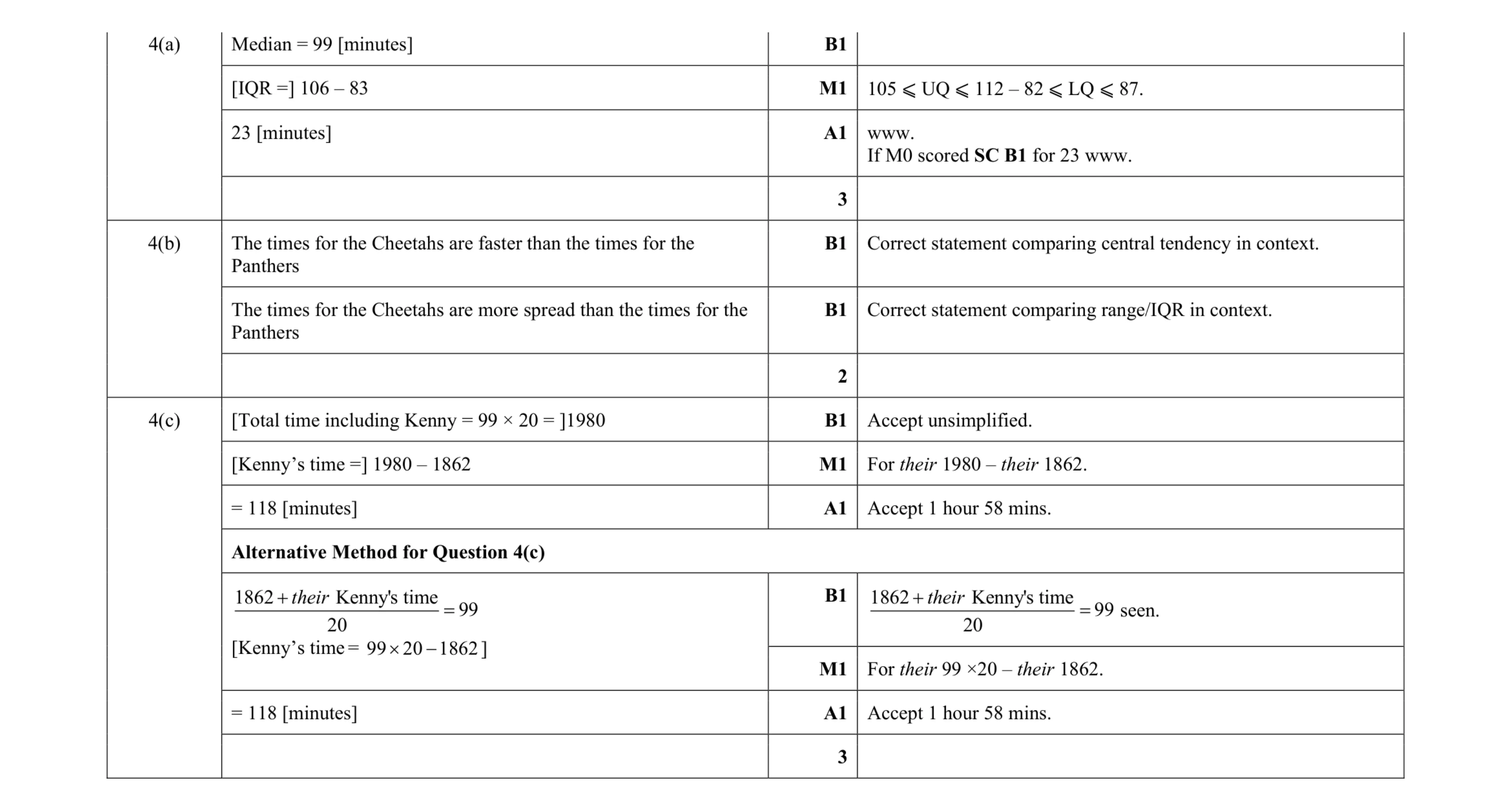 8
8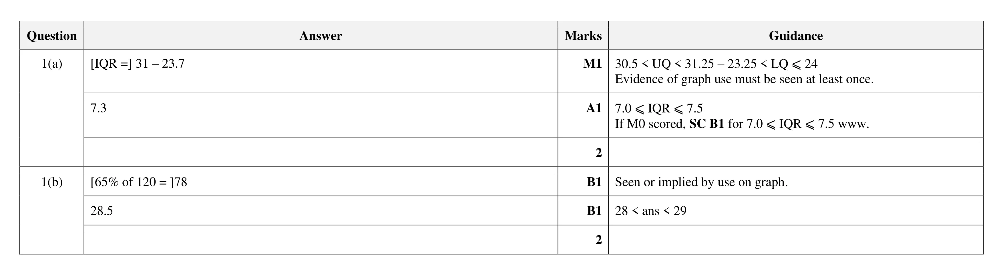 4
4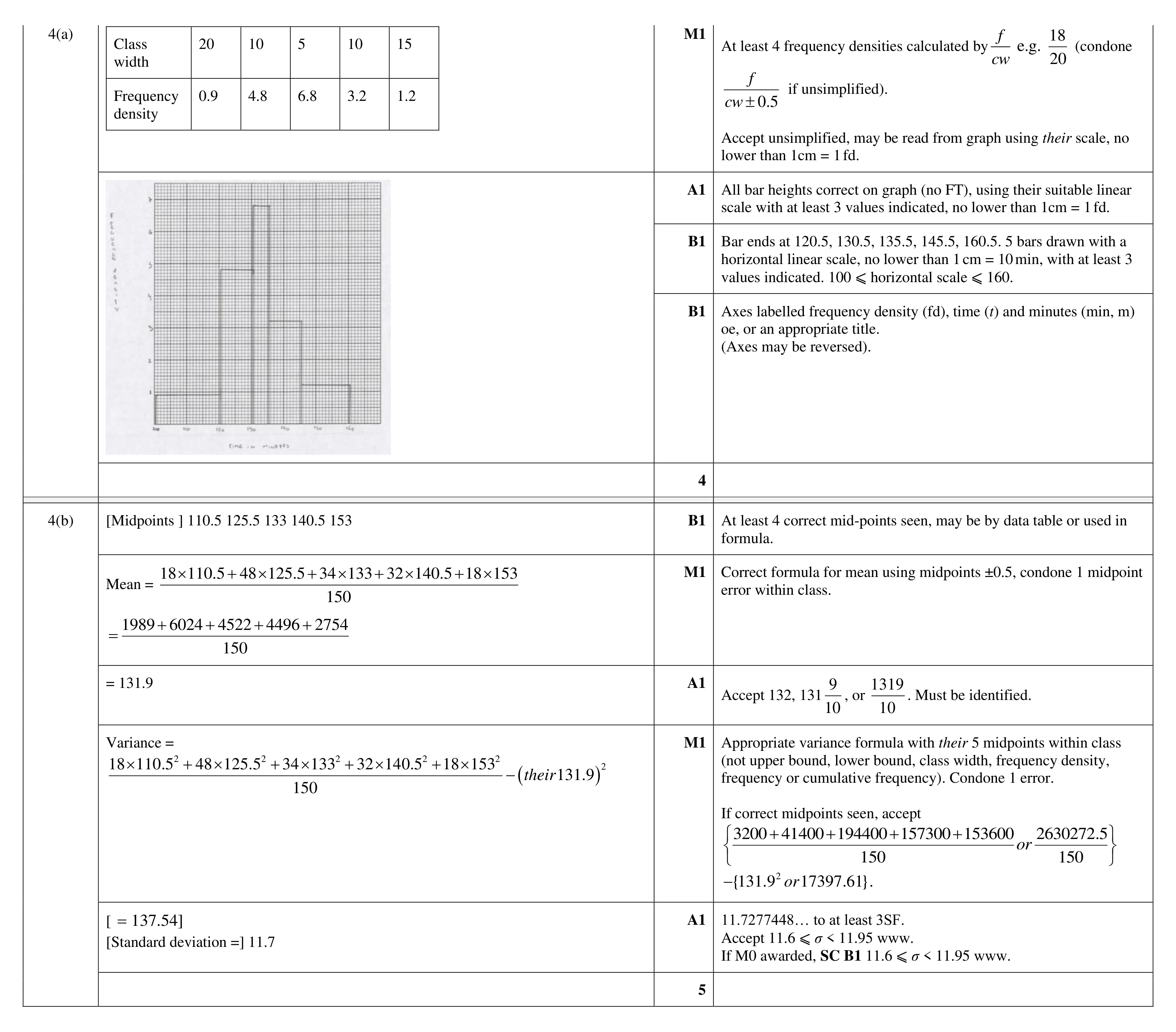 9
9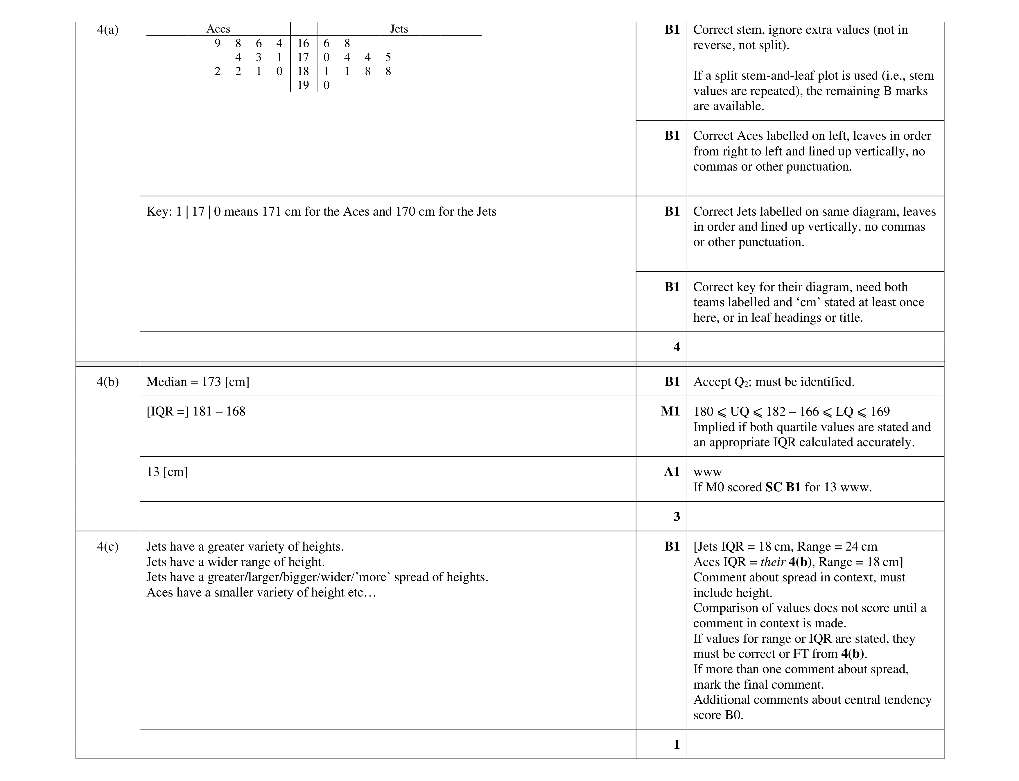 8
8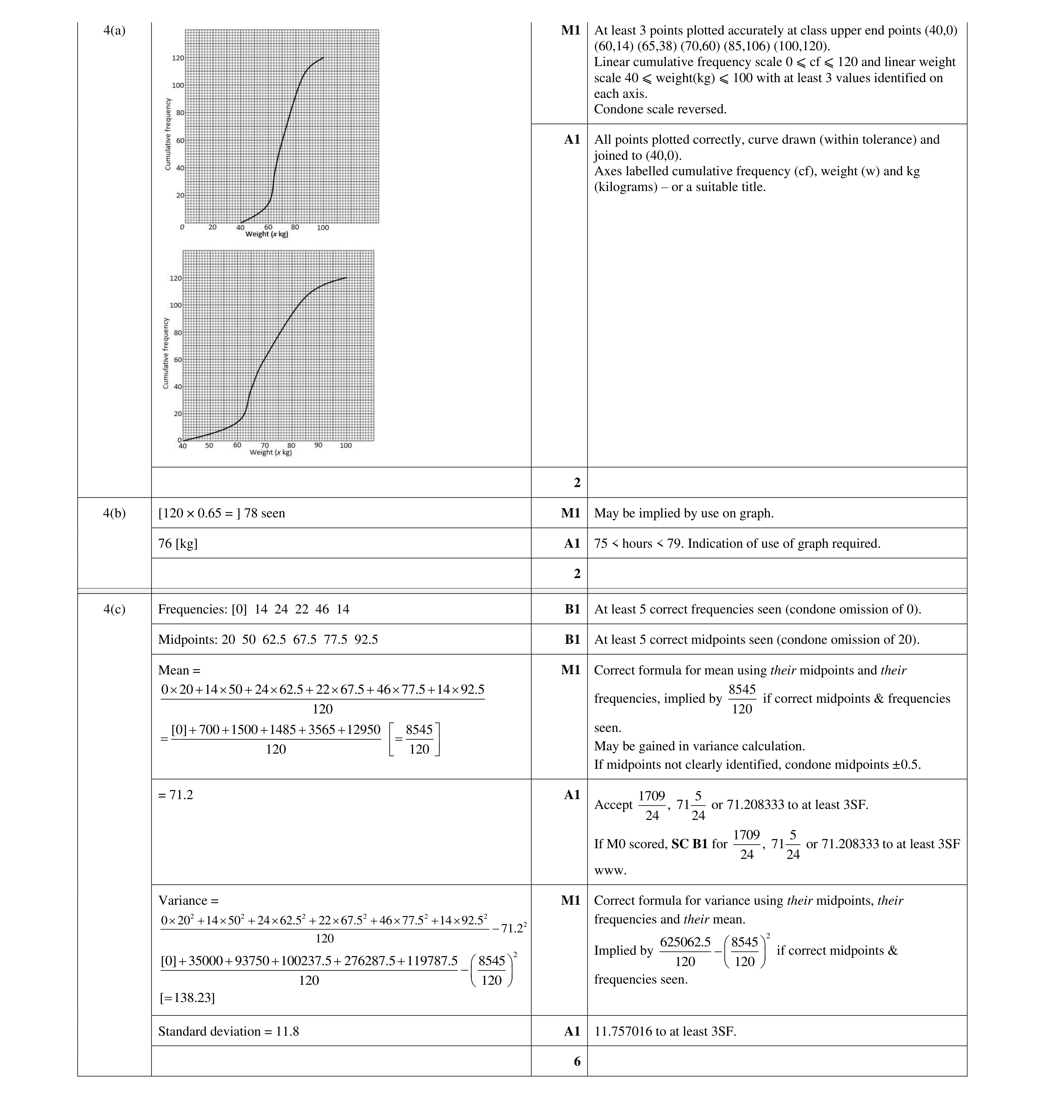 10
10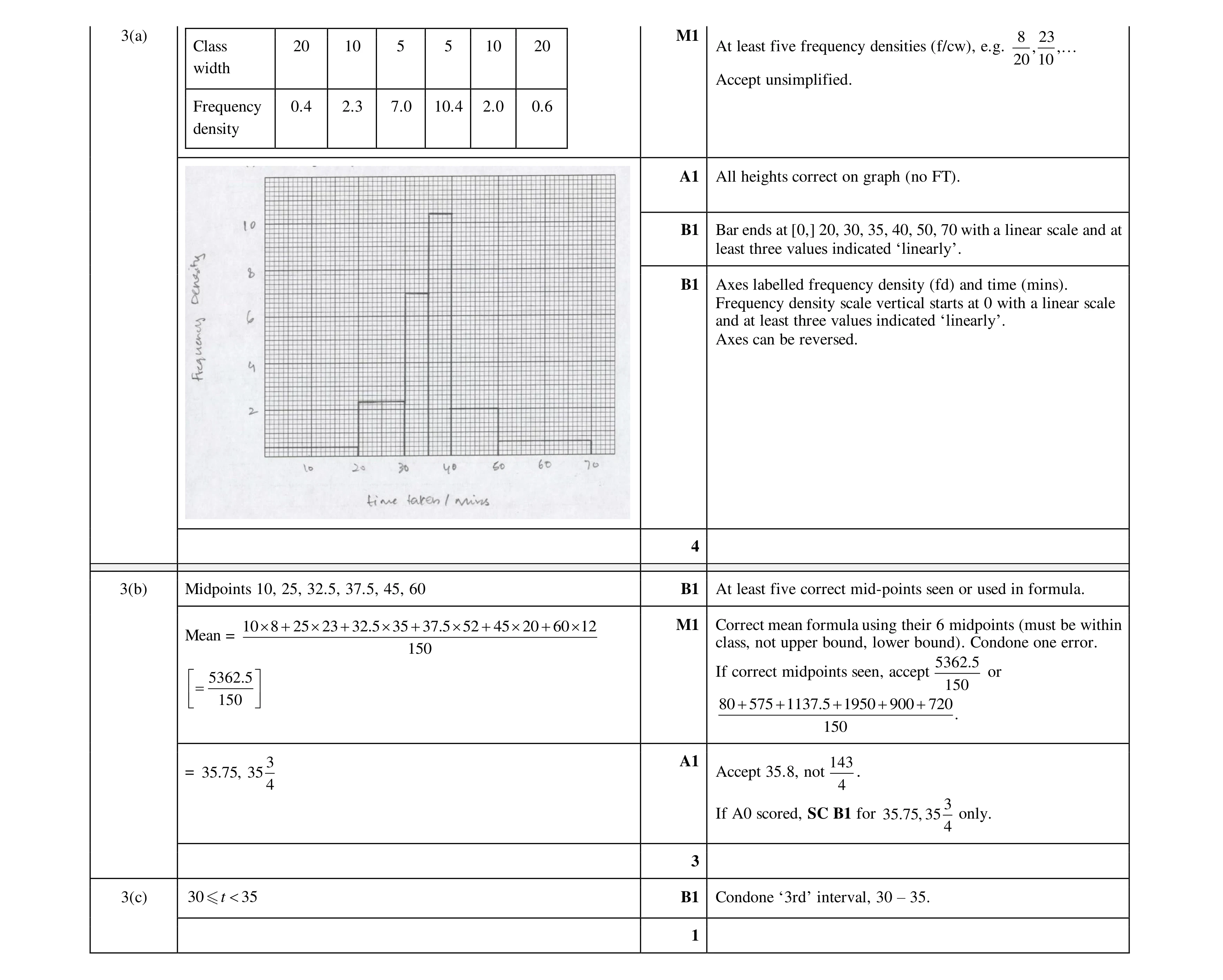 8
8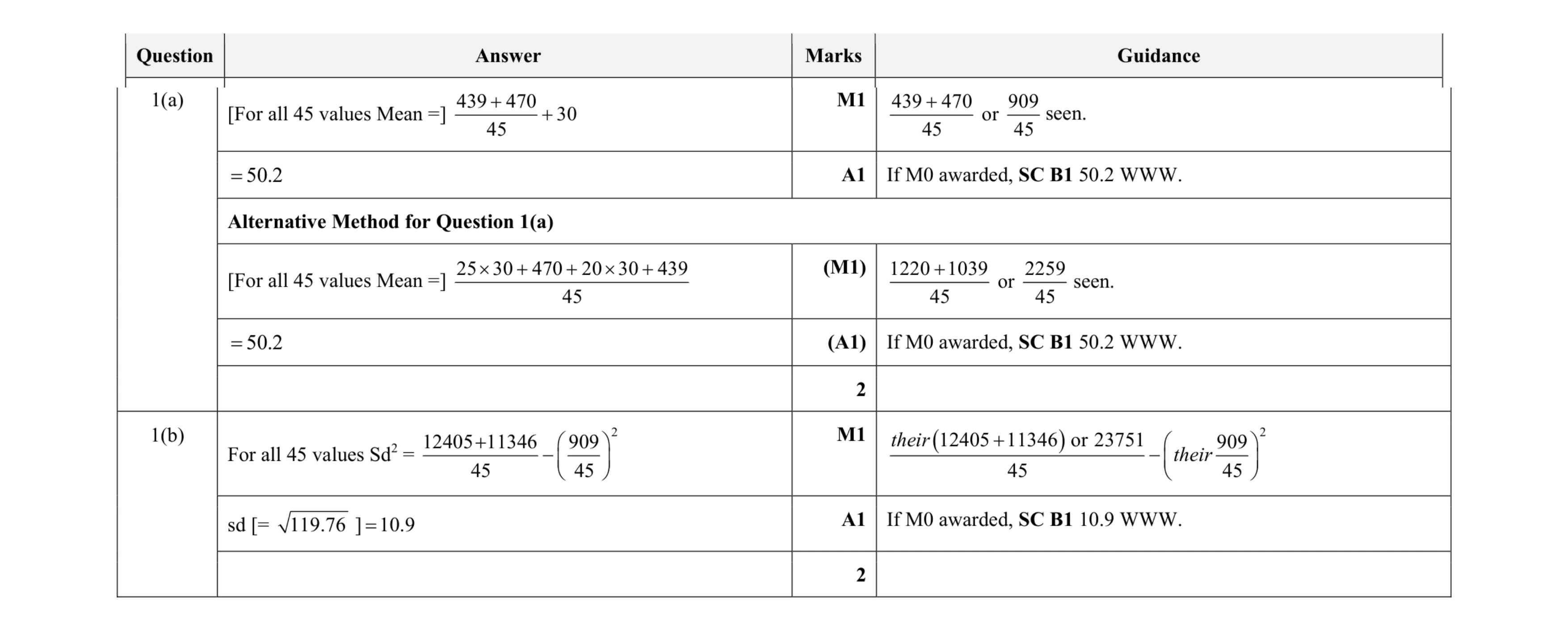 4
4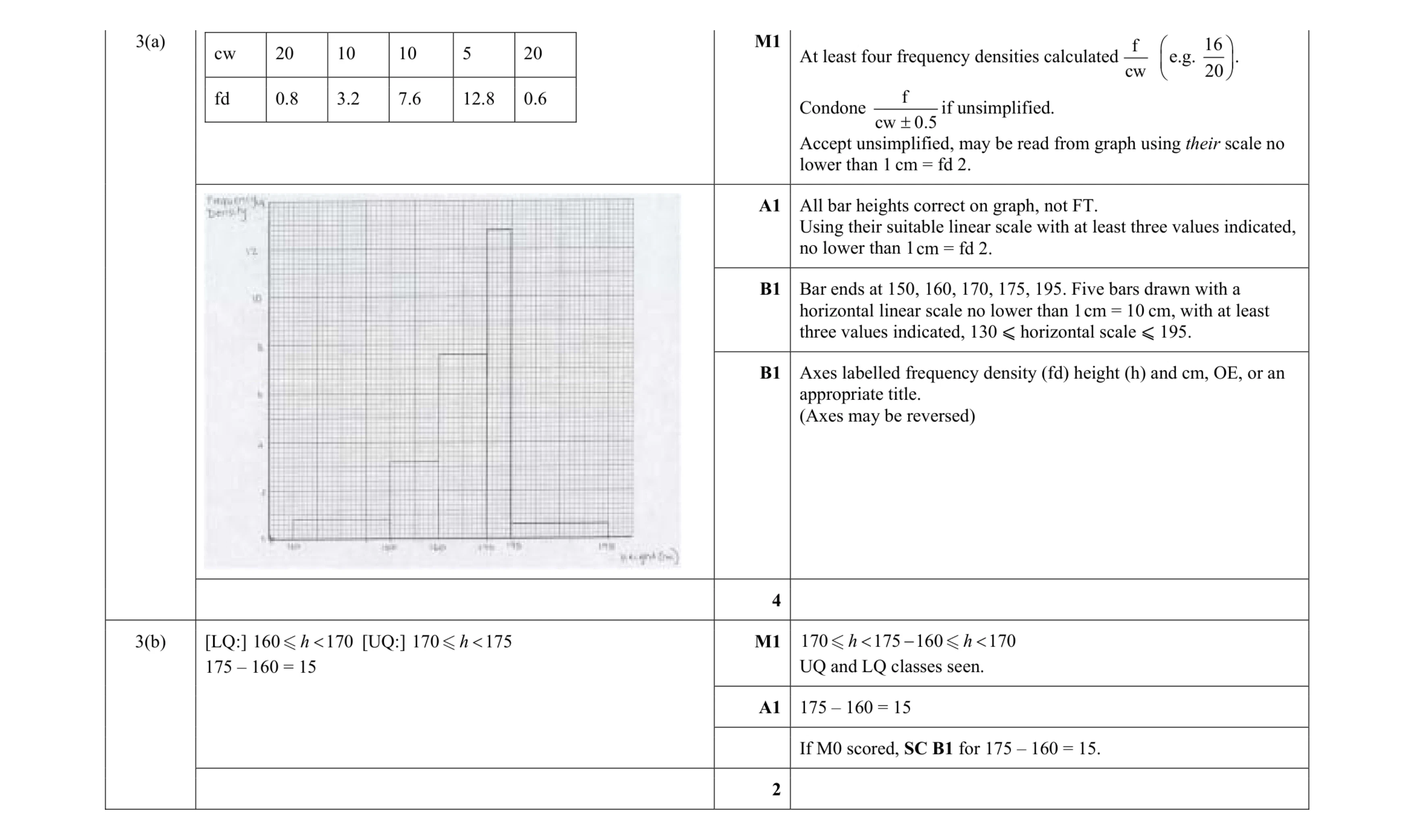 6
6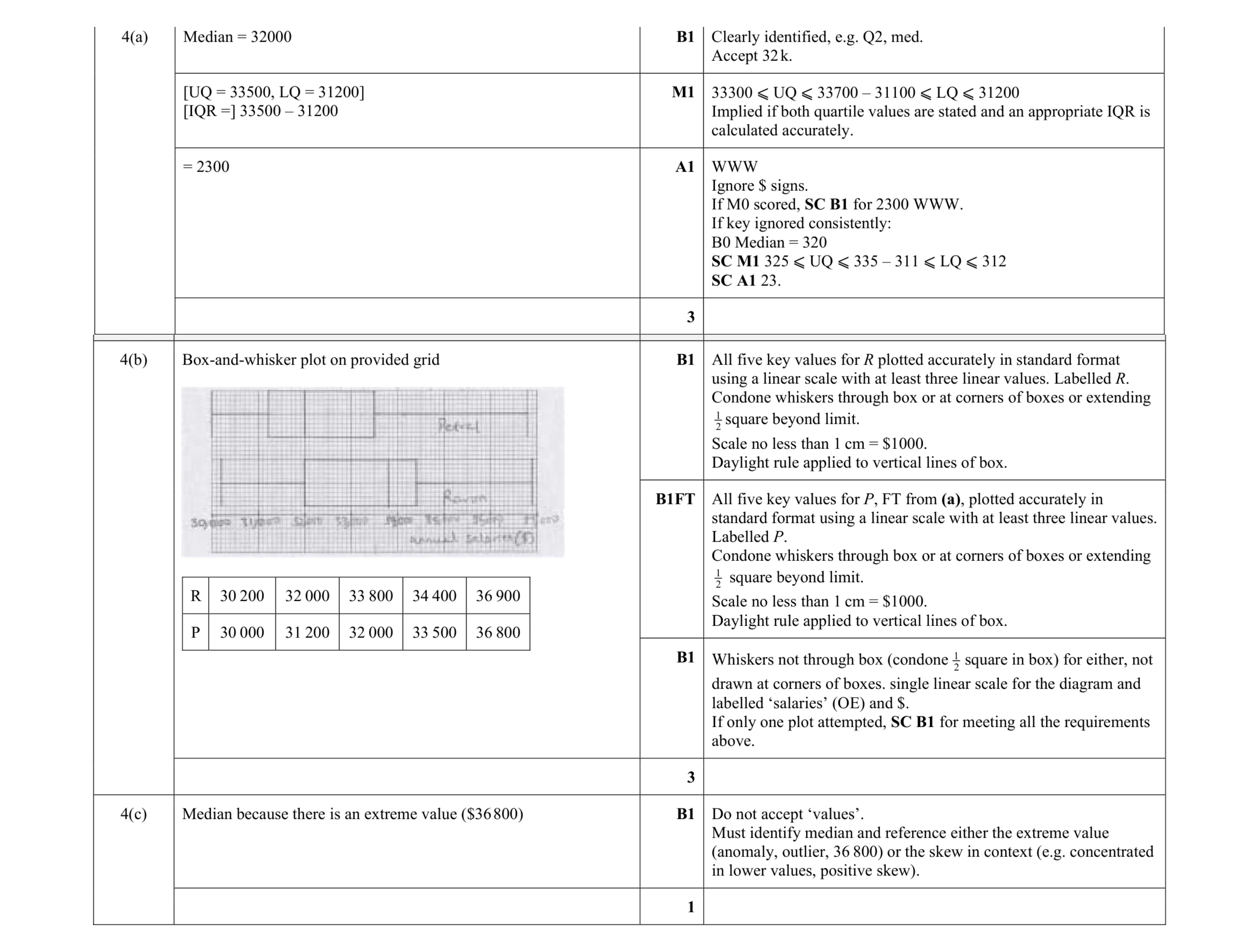 7
7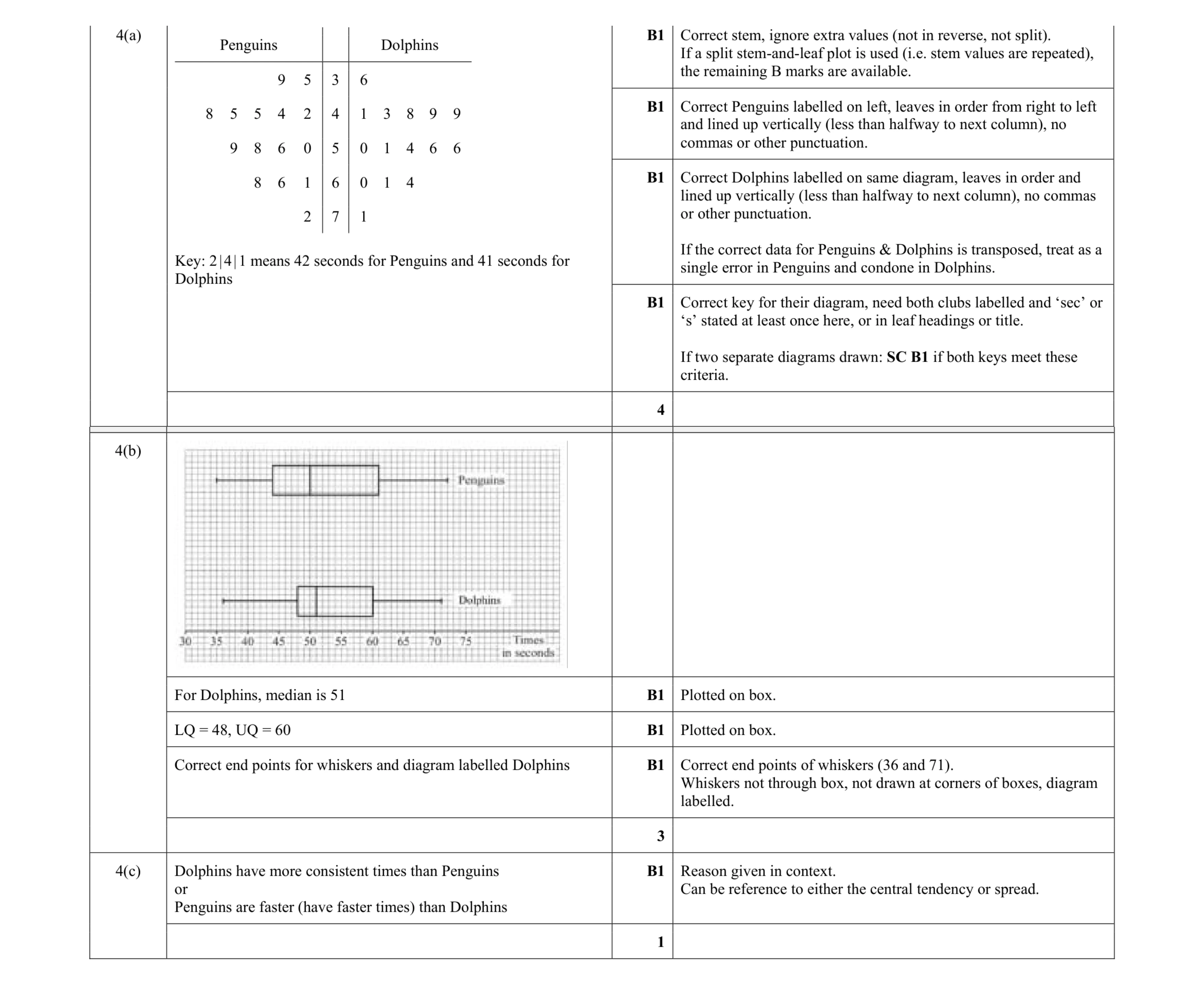 8
8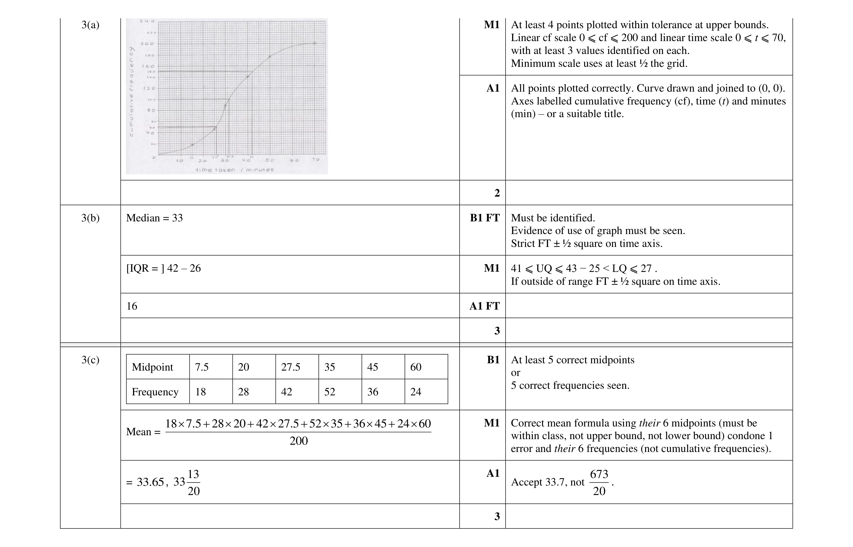 8
8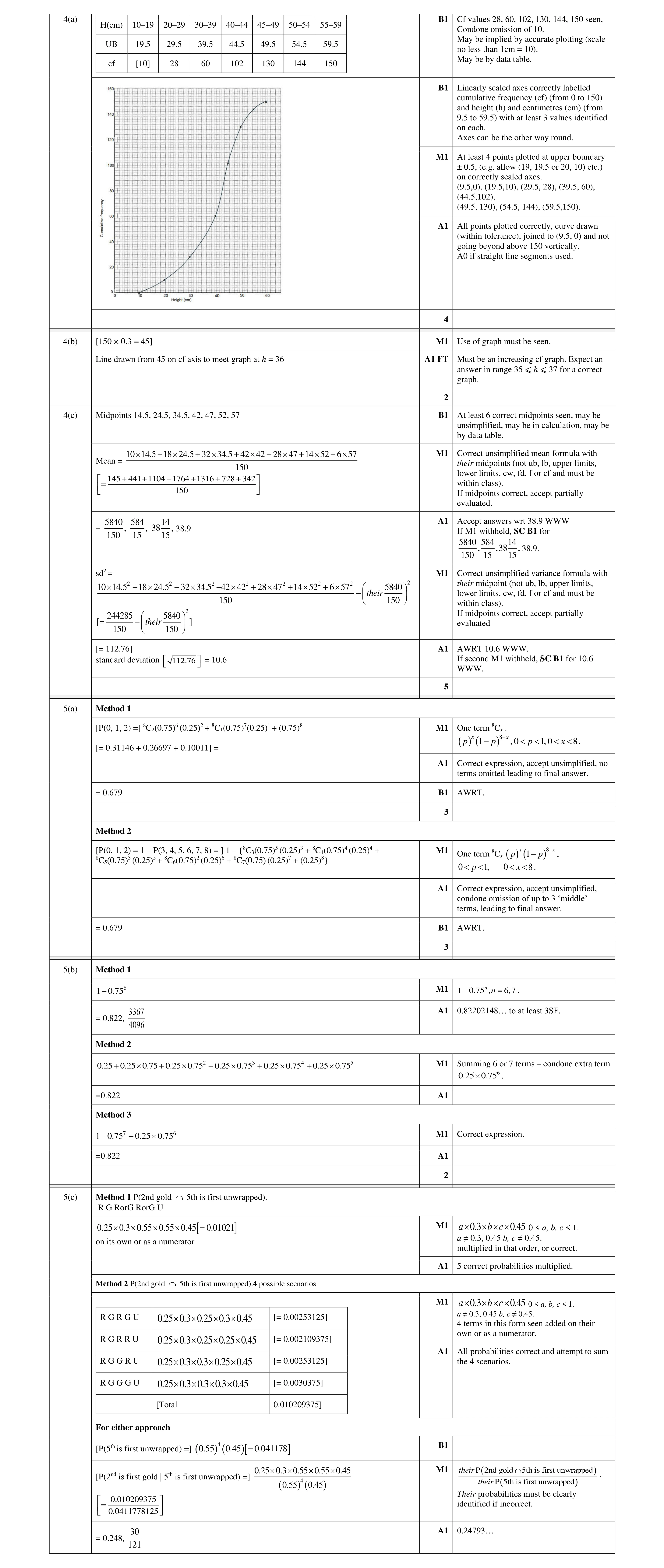 11
11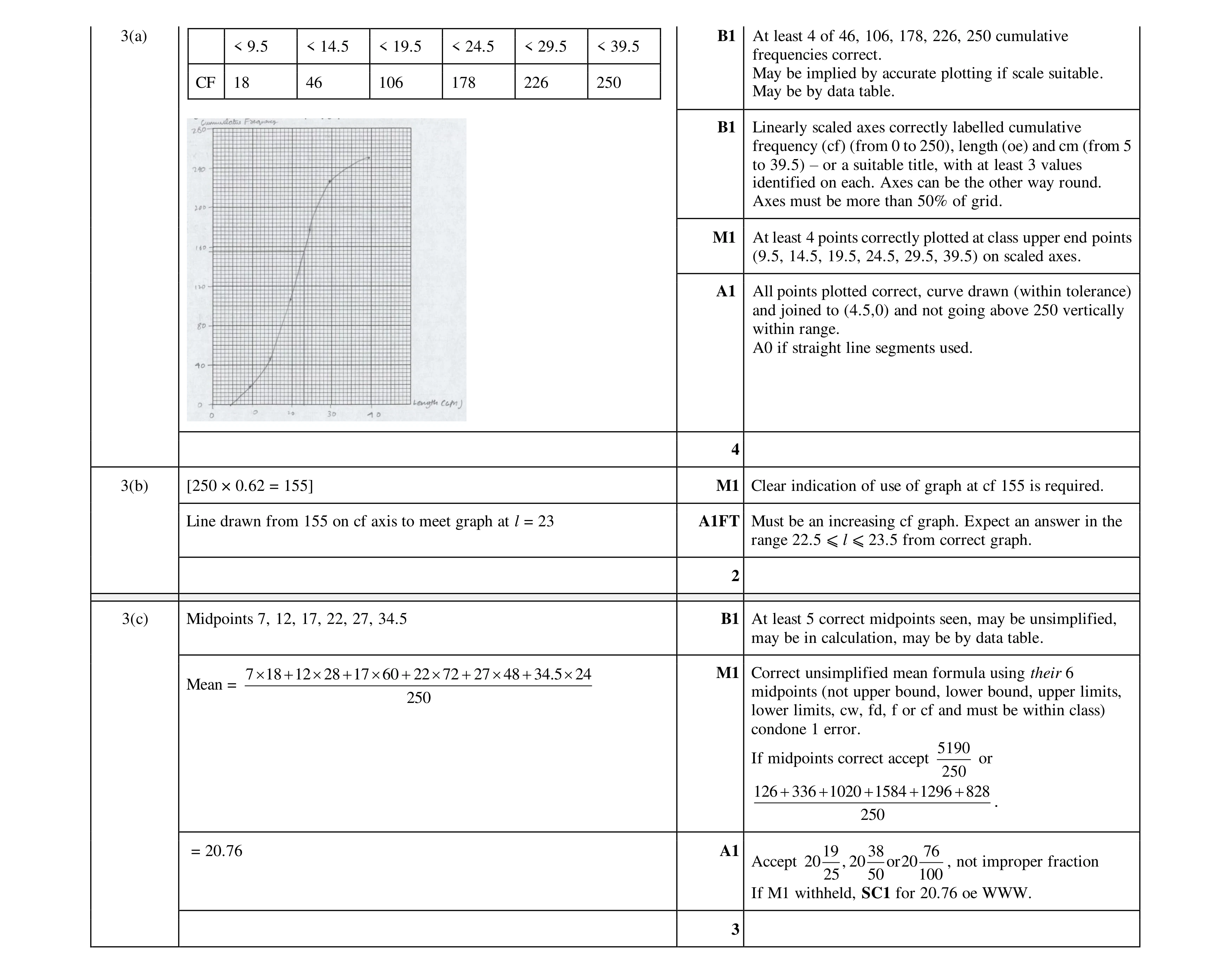 9
9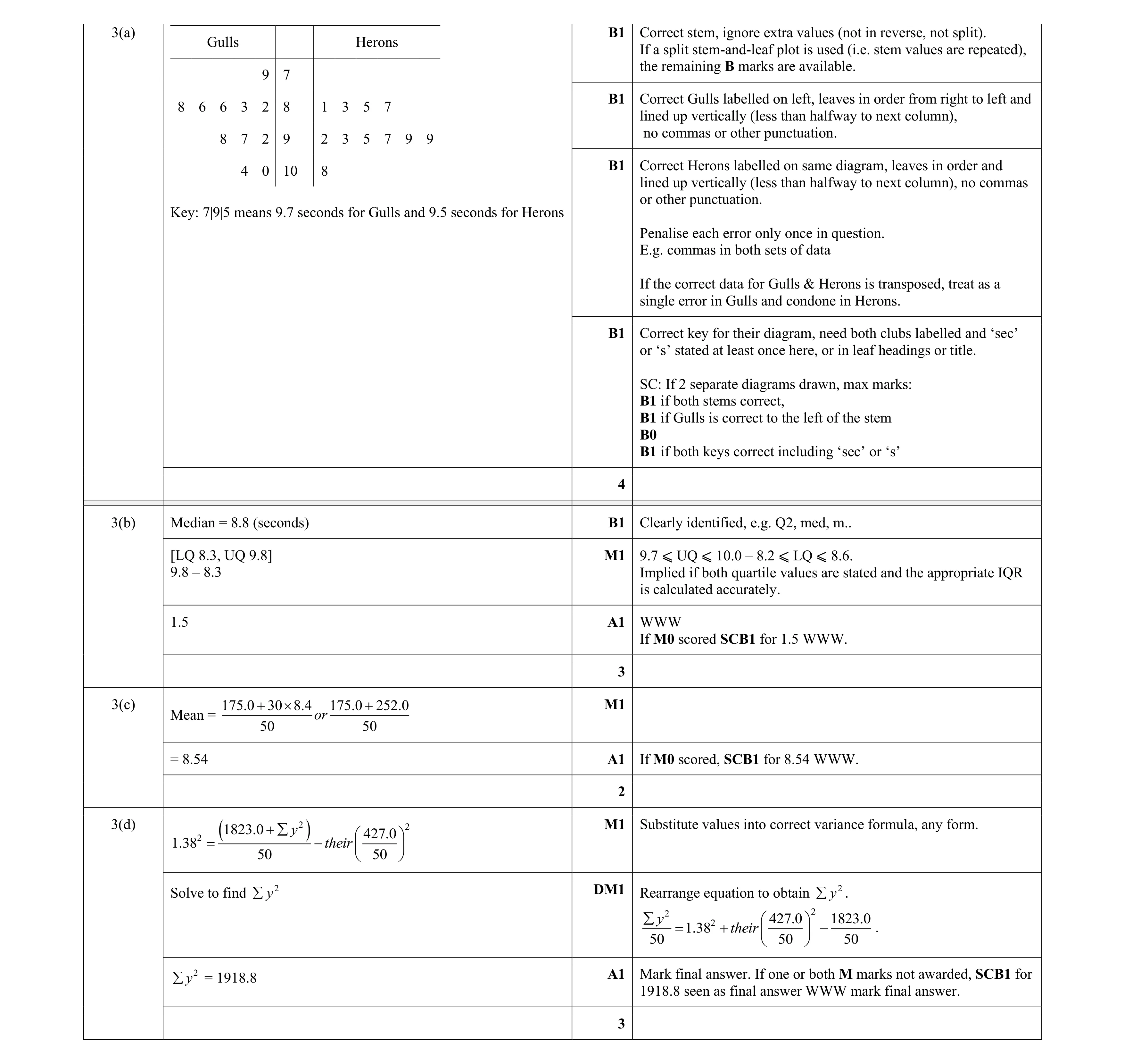 12
12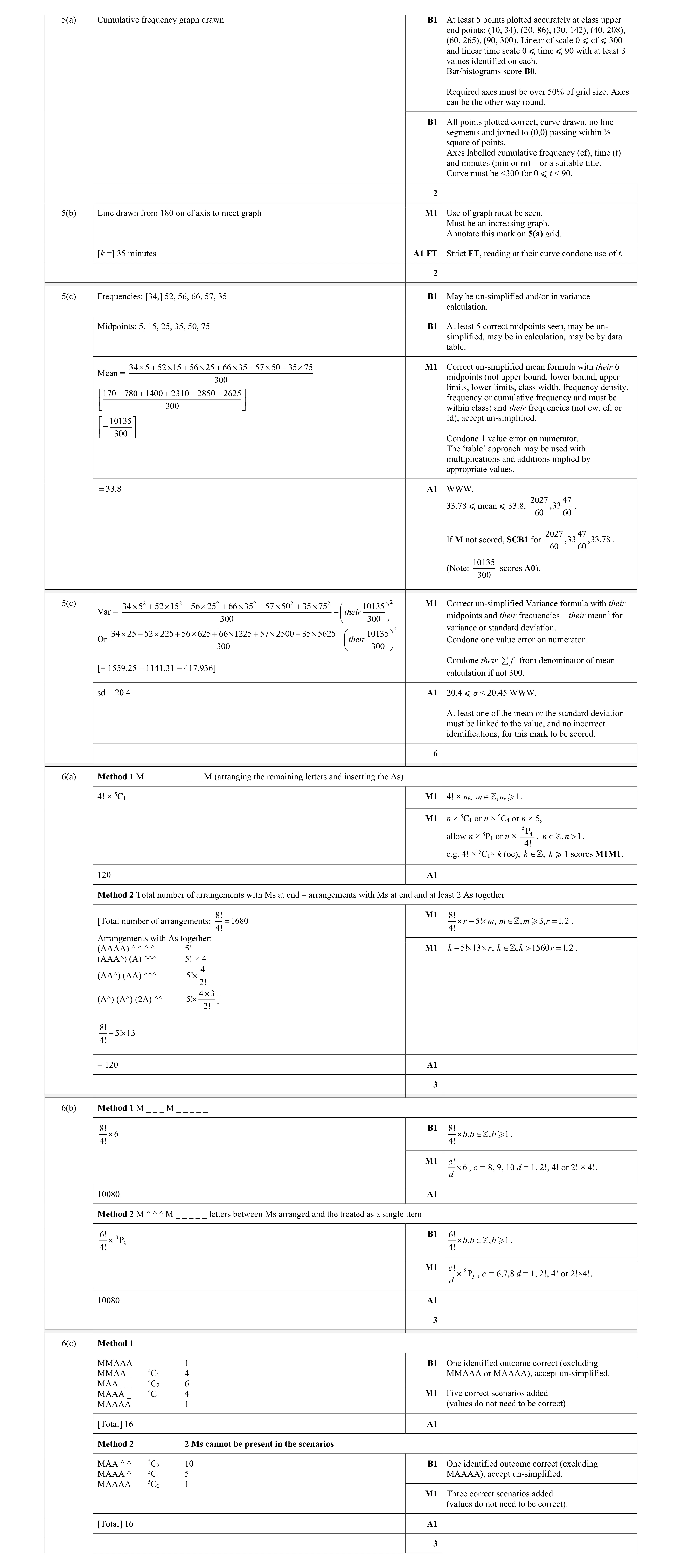 10
10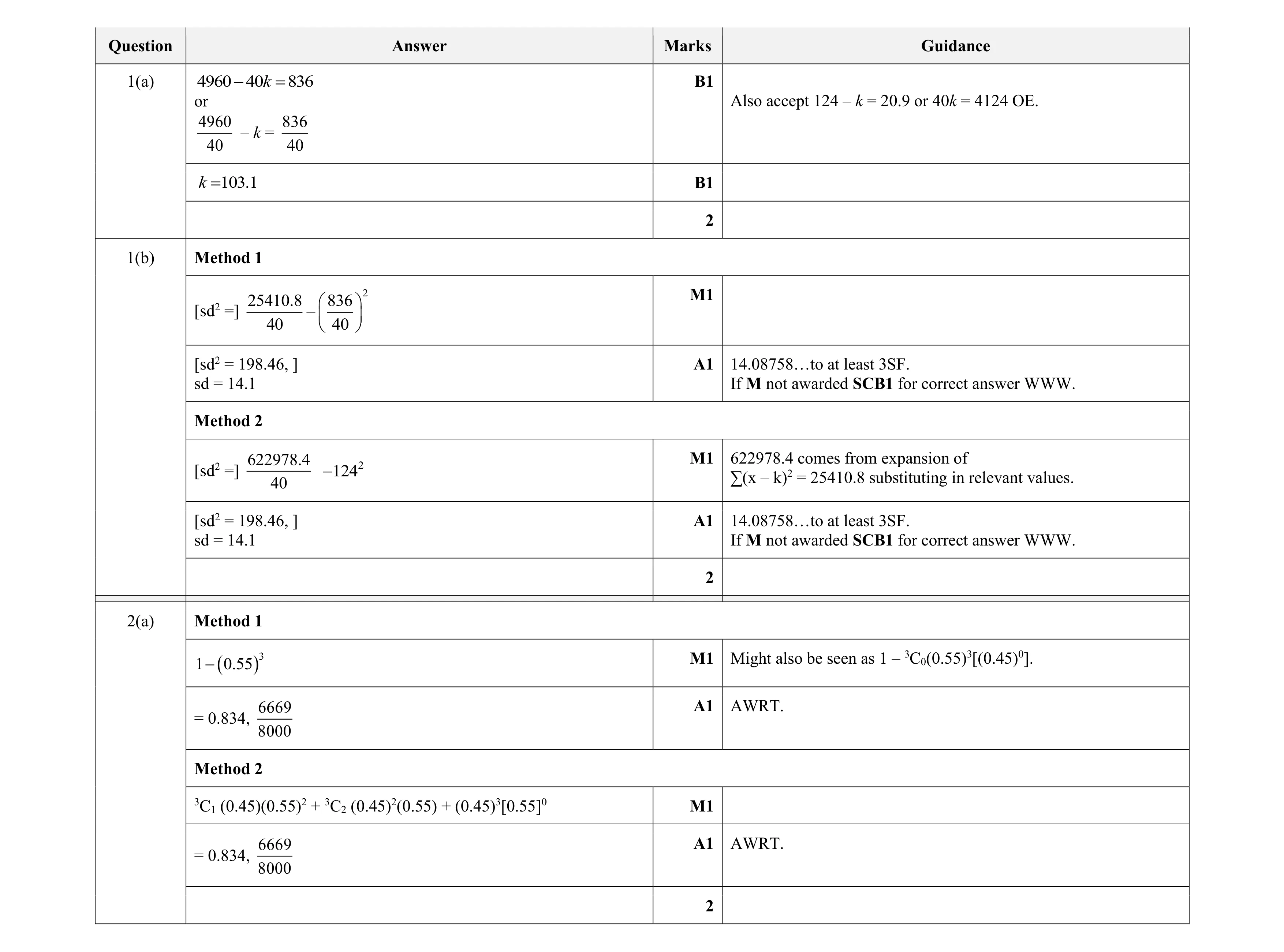 4
4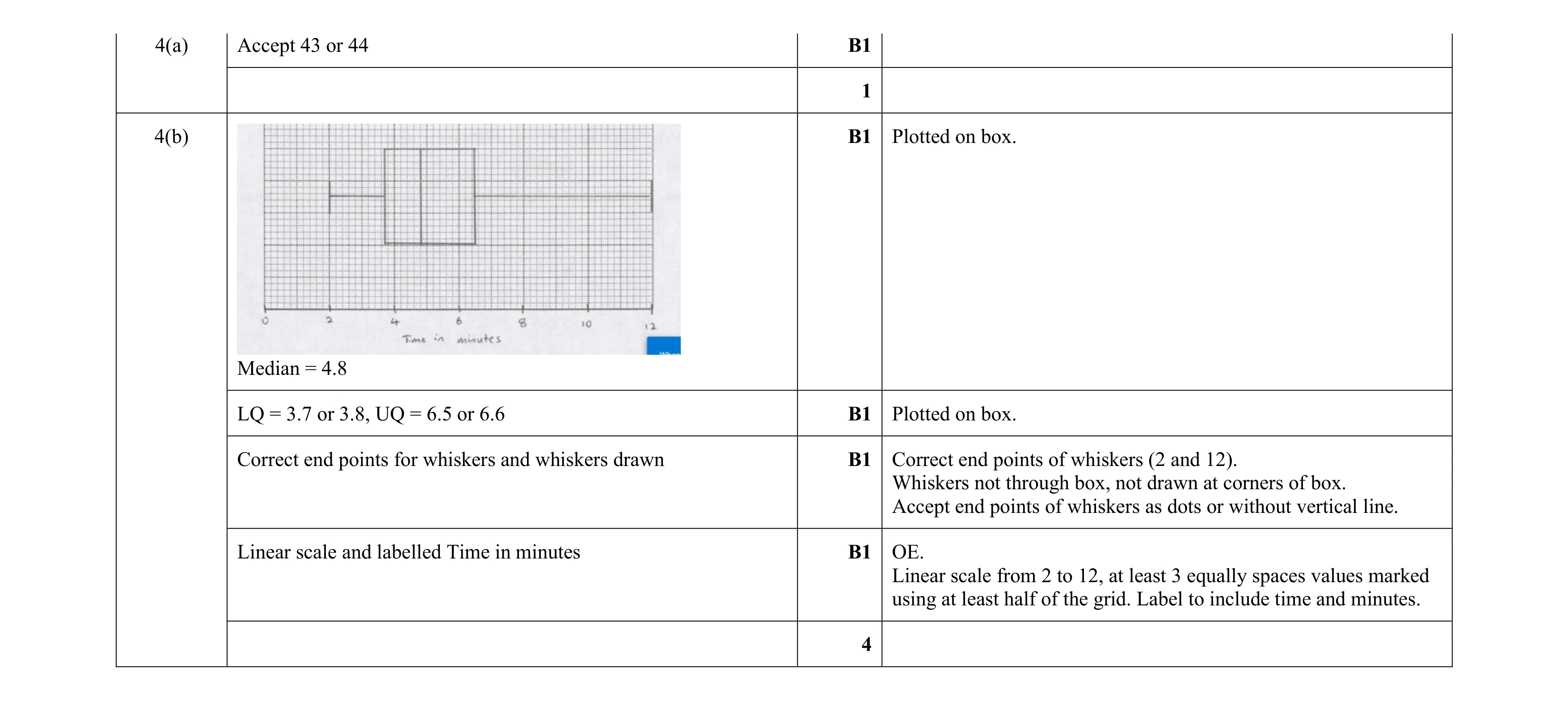 5
5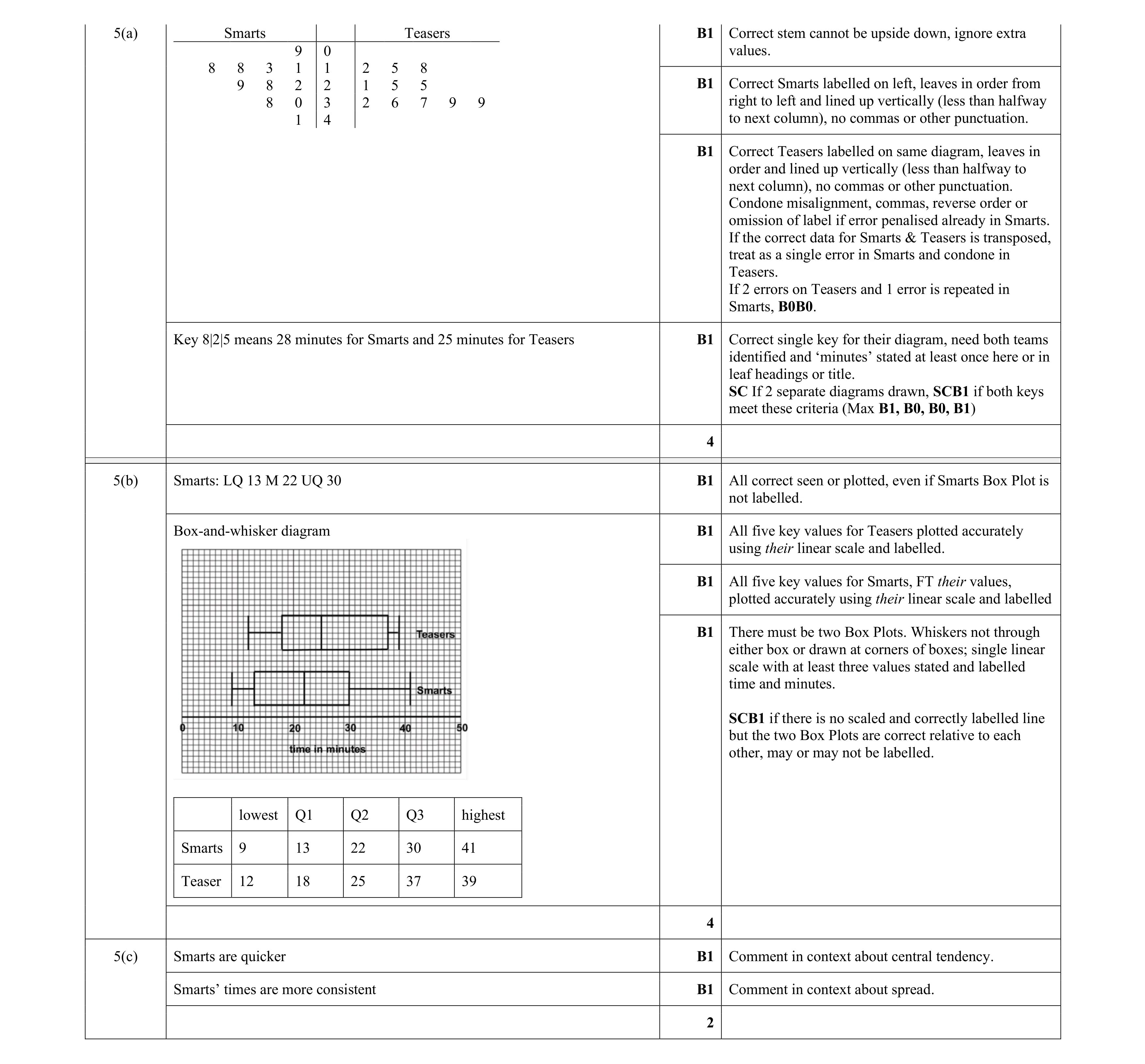 10
10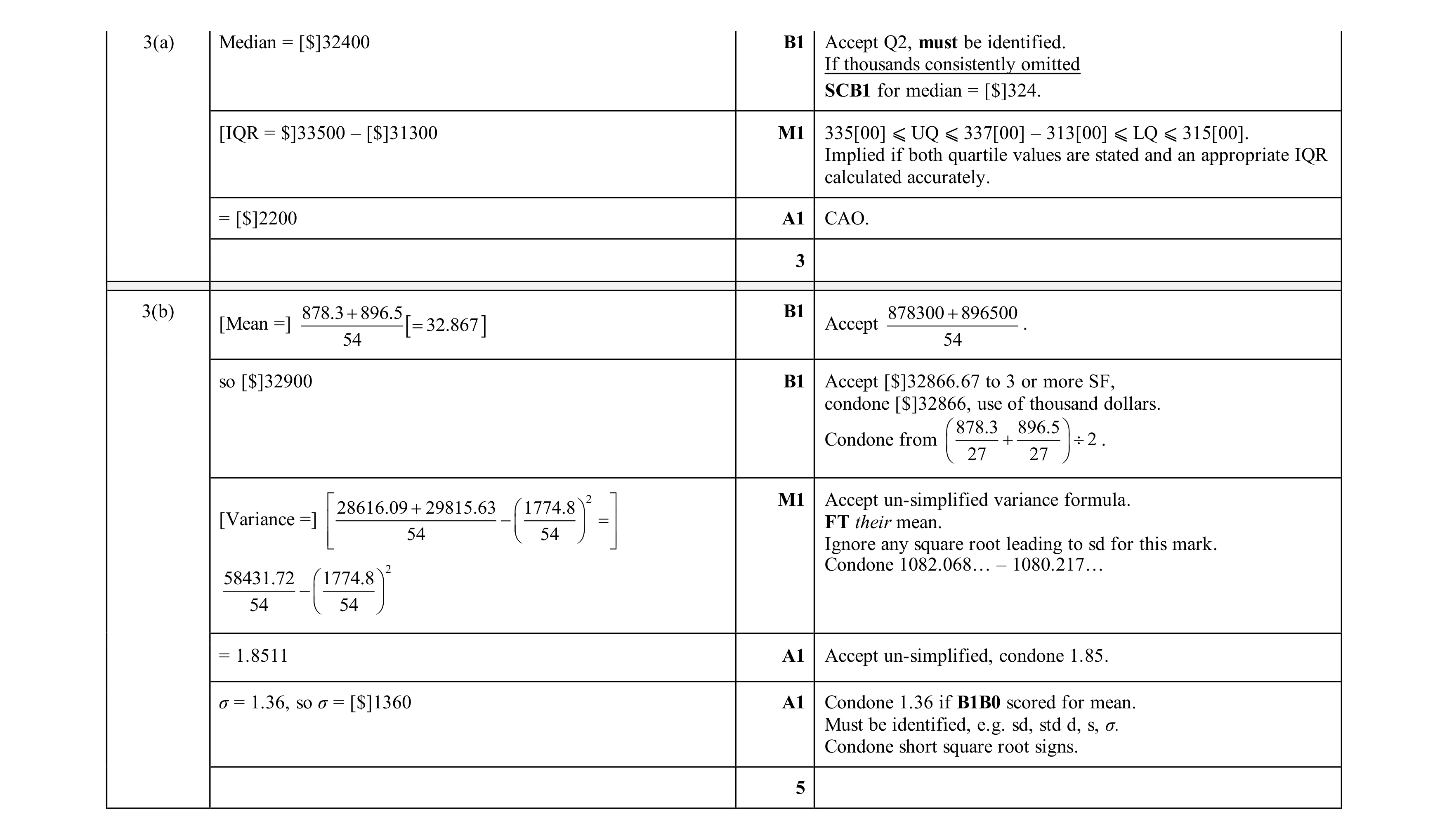 8
8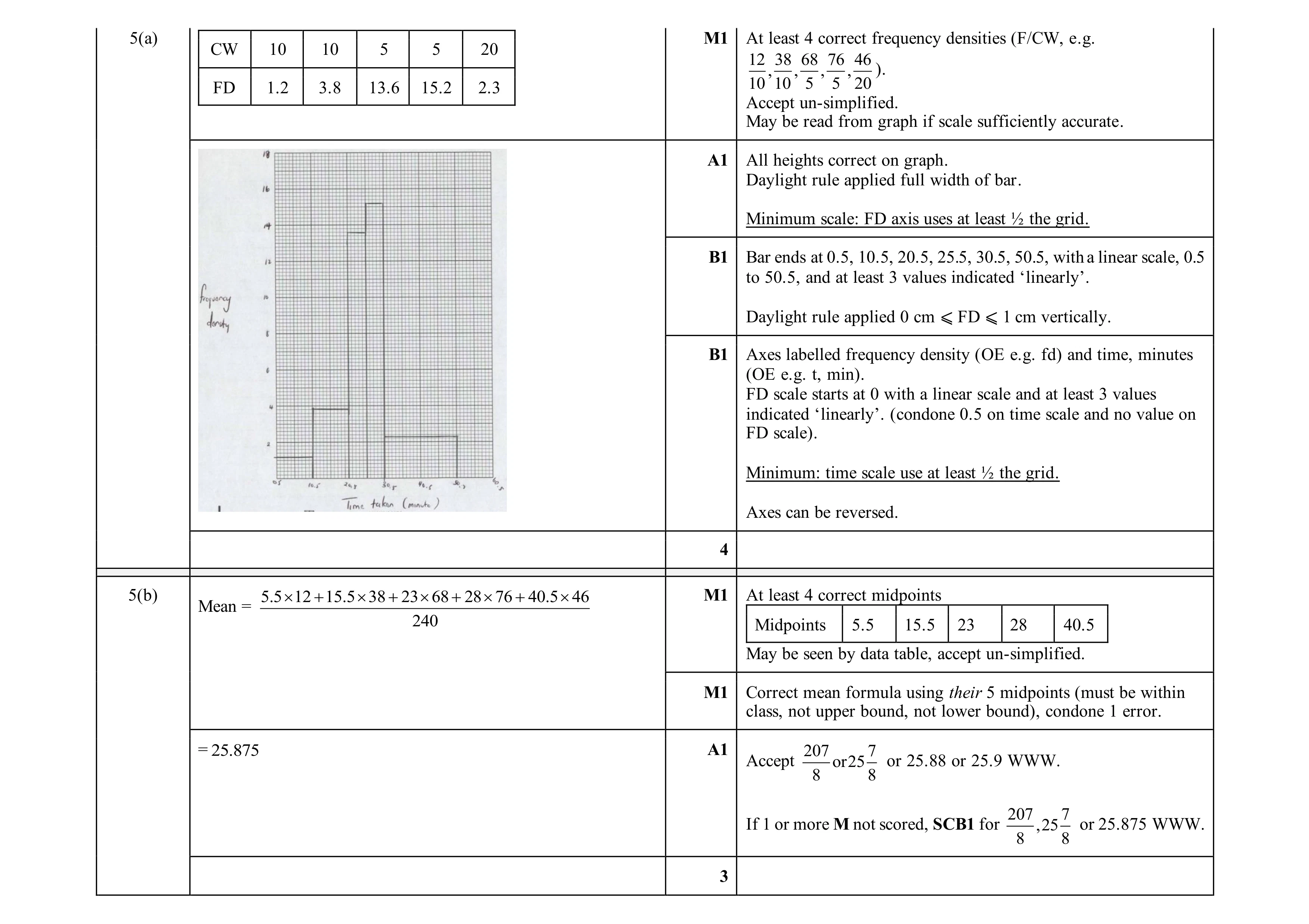 7
7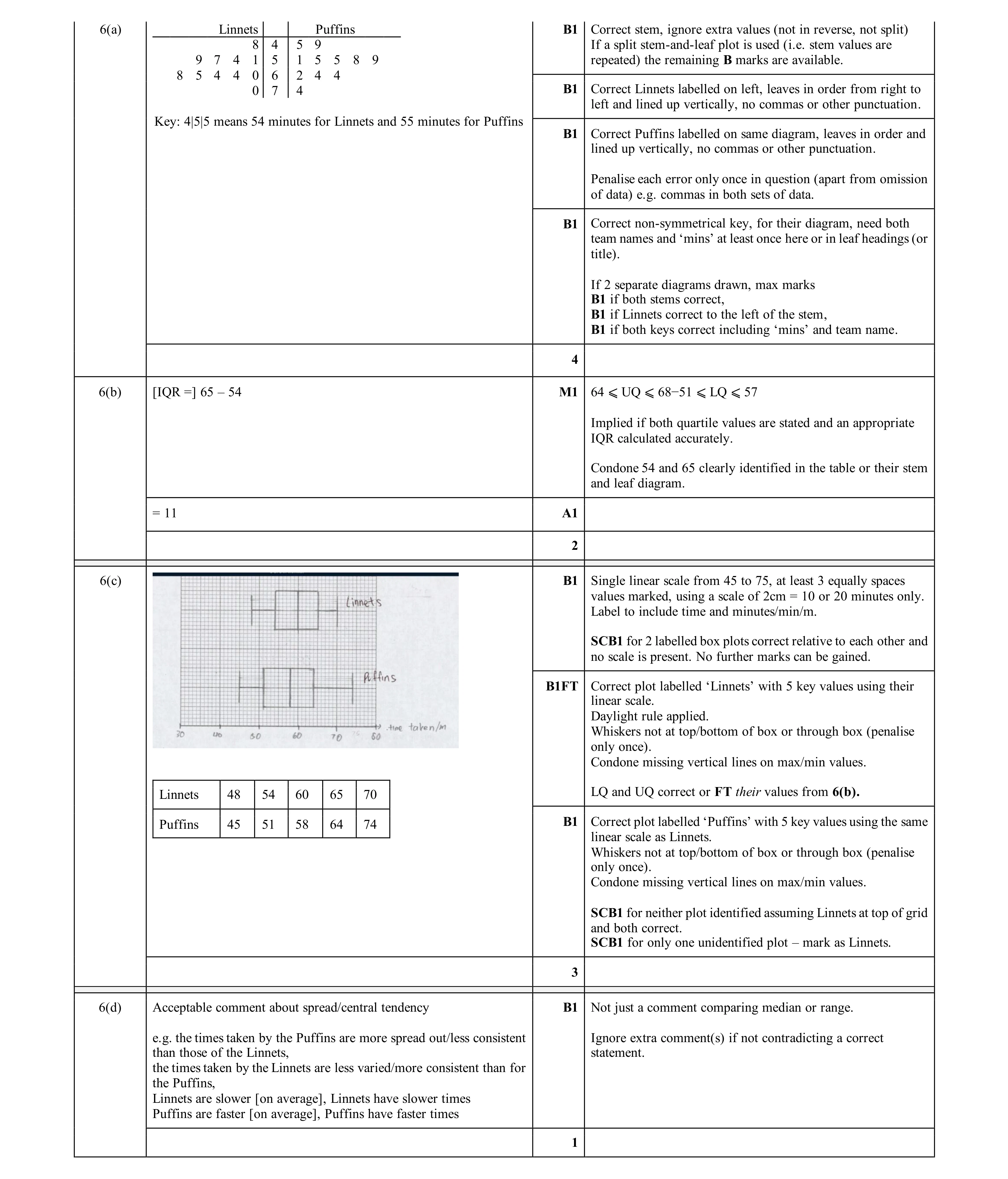 10
10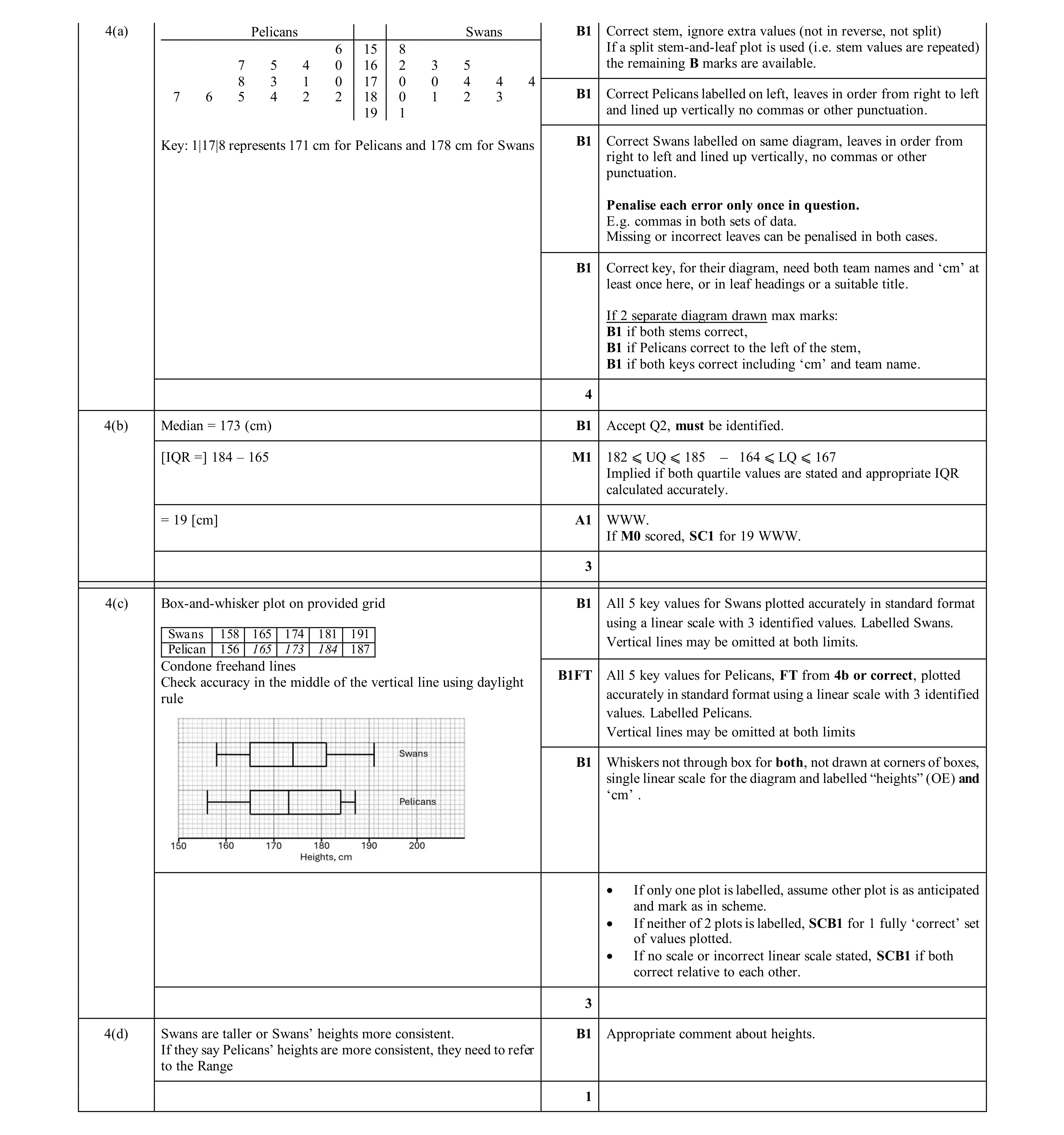 11
11