Questions as text
Q1 · A machine has produced nails over a long period of time, where the length in millimetres… 9709/71 May/June 2007
3 A machine has produced nails over a long period of time, where the length in millimetres was distributed as N(22.0, 0.19). It is believed that recently the mean length has changed. To test this belief a random sample of 8 nails is taken and the mean length is found to be 21.7 mm. Carry out a hypothesis test at the 5% significance level to test whether the population mean has changed, assuming that the variance remains the same. [5]
5 marks
Mark scheme: 2 3 4 2 2(ii) µ = ∫ 3 x / 4 − 3 x / 4 dx =[3 x / 16 − 3 x / 8 ]1 M1 attempt to integrate xf(x), any limits
This question in 9709/71 May/June 2007
Q2 · In Europe the diameters of women’s rings have mean 18.5 mm 9709/71 May/June 2009
1 In Europe the diameters of women’s rings have mean 18.5 mm. Researchers claim that women in Jakarta have smaller fingers than women in Europe. The researchers took a random sample of 20 women in Jakarta and measured the diameters of their rings. The mean diameter was found to be 18.1 mm. Assuming that the diameters of women’s rings in Jakarta have a normal distribution with standard deviation 1.1 mm, carry out a hypothesis test at the 212% level to determine whether the researchers’ claim is justified. [5]
5 marks
Mark scheme: 1 H0 : µ = 18.5 B1 Both hypotheses correct H1 : µ < 18.5 181. − 185. Test statistic z = M1 Standardising, must have 20 1.1( / 20) = –1.626 A1 For correct z CV z = ±1.96 M1 Correct comparison with correct CV or finding area on LHS of –1.626 and comparing with 2.5 % (OR comparison with 2.241 oe if one-tail test set up) Not enough evidence to support the claim A1ft Correct conclusion must ft their CV and their that fingers are smaller. z. No contradictions [5]
This question in 9709/71 May/June 2009
Q3 · In a certain city it is necessary to pass a driving test in order to be allowed to drive… 9709/71 May/June 2009
4 In a certain city it is necessary to pass a driving test in order to be allowed to drive a car. The probability of passing the driving test at the first attempt is 0.36 on average. A particular driving instructor claims that the probability of his pupils passing at the first attempt is higher than 0.36. A random sample of 8 of his pupils showed that 7 passed at the first attempt. (i) Carry out an appropriate hypothesis test to test the driving instructor’s claim, using a significance level of 5%. [5] (ii) In fact, most of this random sample happened to be careful and sensible drivers. State which type of error in the hypothesis test (Type I or Type II) could have been made in these circumstances and find the probability of this type of error when a sample of size 8 is used for the test. [4]
9 marks
Mark scheme: 4 (i) H0 : p = 0.36 B1 Both hypotheses correct H1 : p > 0.36 P(7) = 8C7 × (0.36)7 (0.64)1 = 0.00401 M1 Evaluating P(7) or P(8) P(8) = (0.36)8 = 0.000282 A1 Correct answer for both Σ P = 0.00429 < 0.05 M1 Comparing their prob sum to 0.05 oe Accept driving instructor’s claim B1 Correct conclusion cwo no contradictions [5] (ii) Type I error B1 Correct answer P(6) = 8C6 × (0.36)6 (0.64)2 = 0.02496 M1 Evaluating P(6) P(5) = 8C5 × (0.36)5 (0.64)3 = 0.08876, B1 Correct P(5) and showing this is not in the CR > 0.05 either by Σ P > 0.05 or P(5) > 0.05 P(Type I error) = 0.0292 or 0.0293 A1 Correct answer NB Marks for part (ii) may be awarded in part (i) but not vice versa. [4] 6 ∫ 2
This question in 9709/71 May/June 2009
Q4 · The number of severe floods per year in a certain country over the last 100 years has… 9709/71 Oct/Nov 2009
4 The number of severe floods per year in a certain country over the last 100 years has followed a Poisson distribution with mean 1.8. Scientists suspect that global warming has now increased the mean. A hypothesis test, at the 5% significance level, is to be carried out to test this suspicion. The number of severe floods, X, that occur next year will be used for the test. (i) Show that the rejection region for the test is X 4. [5] > (ii) Find the probability of making a Type II error if the mean number of severe floods is now actually 2.3. [3]
8 marks
Mark scheme: 4 (i) P(X > 4) = 1 – P(0, 1, 2, 3, 4) M1 Adding at least 3 relevant Poisson terms −8.1 8.1 2 8.1 3 8.1 4 M1 Poisson expression for P(X > 4) (oe implied = 1 – e 1 + 8.1 + 2 + !3 + !4 by later working) = 1 – 0.9635 = 0.036(4) A1 Correct prob 0.036 (or 0.96 subject to later working) This is < 0.05 and so X > 4 is in the critical region A1ft Correct comparison and statement identifying CR (ft their prob < 0.05) −8.1 8.1 4 B1 [5] Verification that X = 4 is not in the cr region P(4) = e !4 = 0.0723 (ii) P(Type II error) = P(X = 0, 1, 2, 3, 4) B1 Correct region − 3.2 3.2 2 3.2 3 3.2 4 M1 Poisson expression P(0, 1, 2, 3, 4) = e 1 + 3.2 + 2 + !3 + !4 = 0.916 A1 [3] Correct answer GCE A/AS LEVEL – October/November 2009 9709 71 π / 4 ∫
This question in 9709/71 Oct/Nov 2009
Q5 · Photographers often need to take many photographs of families until they find a photograph… 9709/71 Oct/Nov 2009
6 Photographers often need to take many photographs of families until they find a photograph which everyone in the family likes. The number of photographs taken until obtaining one which everybody likes has mean 15.2. A new photographer claims that she can obtain a photograph which everybody likes with fewer photographs taken. To test at the 10% level of significance whether this claim is justified, the numbers of photographs, x, taken by the new photographer with a random sample of 60 families are recorded. The results are summarised by Σ x 890 and Σ x2 13 780. = = (i) Calculate unbiased estimates of the population mean and variance of the number of photographs taken by the new photographer. [3] (ii) State null and alternative hypotheses for the test, and state also the probability that the test results in a Type I error. Say what a Type I error means in the context of the question. [3] (iii) Carry out the test. [4]
10 marks
Mark scheme: 6 (i) x = 148. (890/60 oe) B1 Correct answer 2 1 890 2 s = 59 13780 − 60 M1 Substituting in formula from book, o.e. = 9.80 A1 [3] Correct answer (ii) H0: µ = 15.2 H1: µ < 15.2 B1 Correct H1 and H0 P(Type I error) = 0.1 (10%) B1 Correct answer Say the photographer has fewer discards when she doesn’t B1ft [3] o.e. must be related to question. No contradictions. ft their H1 14.83 − 152. (iii) Test statistic z = M1 Standardising must have 60 .9802 60 = –0.915 A1 Correct z (±0.91 to 0.92) or correct area 0.18 CV z = ± 1.282 M1 Valid comparison with correct CV must be + with + or – with – and consistent with their H1 oe comparison of areas Not enough evidence to support photographer’s claim. A1ft [4] Correct conclusion ft their z and their CV No contradictions GCE A/AS LEVEL – October/November 2009 9709 71 2
This question in 9709/71 Oct/Nov 2009
Q6 · The masses of packets of cornflakes are normally distributed with standard deviation 11 g 9709/72 Oct/Nov 2009
5 The masses of packets of cornflakes are normally distributed with standard deviation 11 g. A random sample of 20 packets was weighed and found to have a mean mass of 746 g. (i) Test at the 4% significance level whether there is enough evidence to conclude that the population mean mass is less than 750 g. [4] (ii) Given that the population mean mass actually is 750 g, find the smallest possible sample size, n, for which it is at least 97% certain that the mean mass of the sample exceeds 745 g. [4]
8 marks
Mark scheme: 5 (i) H0: µ = 750 H1: µ < 750 B1 H0 and H1 correct 746 − 750 Test statistic z = = +/–1.626 B1 Correct test statistic used in comparison. oe. (11 / 20) CV z = –1.751 or –1.752 M1 Correct CV and valid comparison. oe. [0.0520 or 745.7] [2 tail 2.054/5] Not enough evidence to say mean is less. A1ft Correct conclusion ft their test statistic. [4] No contradictions. Condone cc’s. (ii) z = +/–1.881 or +/–1.882 B1 Accept 1.881 or 1.882 745 − 750 M1* Equation or inequality relating their z to –1.881 > standardised value. Condone cc’s. (11 / n ) M1*dep Solving attempt for n n = 18 A1 Correct answer. cwo. 3 sf accuracy. [4] GCE A/AS LEVEL – October/November 2009 9709 72 2 x ∫ M1 E i 1 d i i
This question in 9709/72 Oct/Nov 2009
Q7 · A hospital patient’s white blood cell count has a Poisson distribution 9709/71 May/June 2010
7 A hospital patient’s white blood cell count has a Poisson distribution. Before undergoing treatment the patient had a mean white blood cell count of 5.2. After the treatment a random measurement of the patient’s white blood cell count is made, and is used to test at the 10% significance level whether the mean white blood cell count has decreased. (i) State what is meant by a Type I error in the context of the question, and find the probability that the test results in a Type I error. [4] (ii) Given that the measured value of the white blood cell count after the treatment is 2, carry out the test. [3] (iii) Find the probability of a Type II error if the mean white blood cell count after the treatment is actually 4.1. [3]
10 marks
Mark scheme: 7 (i) Type I error is made when we say the B1 Correct and relating to question number of white blood cells has decreased when it hasn’t. P(0) = e–5.2 = 0.005516 M1 Evaluating at least 2 of P(X = 0, 1, 2) P(1) = e–5.2(5.2) = 0.02868 Σ < 0.10 M1*Σ Comparing their Σ 3 probs with 10% (must be Σ P(2) = e–5.2(5.22/2) = 0.07458 Σ > 0.10 Σ probs) Σ P(Type I error) = 0.0342 A1dep Correct answer, dep on previous M [4] (ii) H0: λ = 5.2 λ λ H1: λ < 5.2 B1λ Both hypotheses correct λ P(0+1+2) = 0.1087 > 10% 2 not in C Region. M1 Stating 2 is not in the critical region from above, or evaluating P(0, 1, 2) and comparing with 10% again Accept H0. Not enough evidence to say the A1 Correct conclusion no contradictions number of blood cells has decreased. [3] (iii) P(Type II error) = 1 – P(0, 1) B1 Identifying correct area = 1 – e–4.1(1 + 4.1) M1 (indep) Some form of (Poisson) expression with mean 4.1 = 0.915 A1 Correct answer [3]
This question in 9709/71 May/June 2010
Q8 · A hospital patient’s white blood cell count has a Poisson distribution 9709/72 May/June 2010
7 A hospital patient’s white blood cell count has a Poisson distribution. Before undergoing treatment the patient had a mean white blood cell count of 5.2. After the treatment a random measurement of the patient’s white blood cell count is made, and is used to test at the 10% significance level whether the mean white blood cell count has decreased. (i) State what is meant by a Type I error in the context of the question, and find the probability that the test results in a Type I error. [4] (ii) Given that the measured value of the white blood cell count after the treatment is 2, carry out the test. [3] (iii) Find the probability of a Type II error if the mean white blood cell count after the treatment is actually 4.1. [3]
10 marks
Mark scheme: 7 (i) Type I error is made when we say the B1 Correct and relating to question number of white blood cells has decreased when it hasn’t. P(0) = e–5.2 = 0.005516 M1 Evaluating at least 2 of P(X = 0, 1, 2) P(1) = e–5.2(5.2) = 0.02868 Σ < 0.10 M1*Σ Comparing their Σ 3 probs with 10% (must be Σ P(2) = e–5.2(5.22/2) = 0.07458 Σ > 0.10 Σ probs) Σ P(Type I error) = 0.0342 A1dep Correct answer, dep on previous M [4] (ii) H0: λ = 5.2 λ λ H1: λ < 5.2 B1λ Both hypotheses correct λ P(0+1+2) = 0.1087 > 10% 2 not in C Region. M1 Stating 2 is not in the critical region from above, or evaluating P(0, 1, 2) and comparing with 10% again Accept H0. Not enough evidence to say the A1 Correct conclusion no contradictions number of blood cells has decreased. [3] (iii) P(Type II error) = 1 – P(0, 1) B1 Identifying correct area = 1 – e–4.1(1 + 4.1) M1 (indep) Some form of (Poisson) expression with mean 4.1 = 0.915 A1 Correct answer [3]
This question in 9709/72 May/June 2010
Q9 · At the 2009 election, 13 of the voters in Chington voted for the Citizens Party 9709/73 May/June 2010
1 At the 2009 election, 13 of the voters in Chington voted for the Citizens Party. One year later, a researcher questioned 20 randomly selected voters in Chington. Exactly 3 of these 20 voters said that if there were an election next week they would vote for the Citizens Party. Test at the 2.5% significance level whether there is evidence of a decrease in support for the Citizens Party in Chington, since the 2009 election. [5]
5 marks
Mark scheme: 1 H0: Pop prop = 1/3 (or unchanged) H1: Pop prop < 1/3 (or decreased) B1 Accept p 2 2 1 2 1 ( )20 + 30( )19( ) + 20C2( )18( )2 M1 Attempt Bin(20, ⅓) P(Y 3) 3 3 3 3 3 2 1 + 20C3( )17( )3 Allow one term omitted 3 3 = 0.0604/0.0605 A1 comp “0.0604” with 0.025 M1 For comparison of their 0.0604 No evidence that support decreased or support probably not decreased A1ft Correct conclusion no contradictions [5] SC Use Of Normal Standardising with or without cc M1 Obtains z = –1.502 A1 Valid Comparison with z = –1.96 M1 Correct conclusion A1ft
This question in 9709/73 May/June 2010
Q10 · Dipak carries out a test, at the 10% significance level, using a normal distribution 9709/73 May/June 2010
2 Dipak carries out a test, at the 10% significance level, using a normal distribution. The null hypothesis is µ = 35 and the alternative hypothesis is µ ≠35. (i) Is this a one-tail or a two-tail test? State briefly how you can tell. [1] Dipak finds that the value of the test statistic is ß = −1.750. (ii) Explain what conclusion he should draw. [2] (iii) This result is significant at the α% level. Find the smallest possible value of α, correct to the nearest whole number. [2]
5 marks
Mark scheme: 2 (i) 2-tail; H1: µ ¸ 35 B1 [1] (ii) comp –1.75 with –1.645 (or 1.75 with 1.645) M1 Evidence that µ is not 35 A1 Allow “Accept µ ¸ 35”. No contradictions or reject µ = 35 [2] (iii) 8 B2 SR B1 for 4, 8.02, or 92% [2]
This question in 9709/73 May/June 2010
Q11 · At a power plant, the number of breakdowns per year has a Poisson distribution 9709/73 May/June 2010
4 At a power plant, the number of breakdowns per year has a Poisson distribution. In the past the mean number of breakdowns per year has been 4.8. Following some repairs, the management carry out a hypothesis test at the 5% significance level to determine whether this mean has decreased. If there is at most 1 breakdown in the following year, they will conclude that the mean has decreased. (i) State what is meant by a Type I error in this context. [1] (ii) Find the probability of a Type I error. [2] (iii) Find the probability of a Type II error if the mean is now 0.9 breakdowns per year. [3]
6 marks
Mark scheme: 4 (i) Mean is 4.8 but Y 1 breakdown B1 Accept reduction when none has occurred [1] (ii) e–4.8(1 + 4.8) M1 Poisson attempt at P(0) (+ P(1)) = 0.0477 A1 [2] (iii) P(X > 1) M1 Attempt correct probability for Type II error = 1 – e–0.9(1 + 0.9) M1 Allow any λ except 4.8; 1– (P(0)+(P(1))) using Poisson = 0.228 (3 sfs) A1 As final answer [3] ∞ k ∫
This question in 9709/73 May/June 2010
Q12 · The marks of candidates in Mathematics and English in 2009 were represented by the… 9709/71 Oct/Nov 2010
5 The marks of candidates in Mathematics and English in 2009 were represented by the independent random variables X and Y with distributions N(28, 5.62) and N(52, 12.42) respectively. Each candidate’s marks were combined to give a final mark F, where F = X + 12Y. (i) Find E(F) and Var(F). [3] (ii) The final marks of a random sample of 10 candidates from Grinford in 2009 had a mean of 49. Test at the 5% significance level whether this result suggests that the mean final mark of all candidates from Grinford in 2009 was lower than elsewhere. [5]
8 marks
Mark scheme: 5 (i) E(F) = 28 + 1/2 × 52 = 54 B1 Var(F) = 5.62 + 1/4 × 12.42 M1 = 69.8 A1 [3] √69.8 or 8.35: M1A0 (ii) H0: Grinford mean = 54; B1ft Allow “µ”, otherwise undefined H1; Grinford mean < 54 mean: B0 ft their 54 49 − 54 698. M1 Standardising must have √10 10 = –1.89(3) or –1,89(2) allow + A1 Comp with –1.645 (or 1.893 with 1.645) M1 Comp P(z < –1.893) with 0.05 Allow comparison with 1.96 for consistent 2-tail test Evidence that Grinford mean lower A1ft [5] Allow “Accept Grinford mean lower” No contradictions OR Alt methods (x – 54)/(√(69.8/10)) = 1.645 giving x = 49.65 compare with 49 scores M1A1M1A1ft. oe. No mixed methods. GCE A LEVEL – October/November 2010 9709 71 1 1
This question in 9709/71 Oct/Nov 2010
Q13 · The marks of candidates in Mathematics and English in 2009 were represented by the… 9709/72 Oct/Nov 2010
5 The marks of candidates in Mathematics and English in 2009 were represented by the independent random variables X and Y with distributions N(28, 5.62) and N(52, 12.42) respectively. Each candidate’s marks were combined to give a final mark F, where F = X + 12Y. (i) Find E(F) and Var(F). [3] (ii) The final marks of a random sample of 10 candidates from Grinford in 2009 had a mean of 49. Test at the 5% significance level whether this result suggests that the mean final mark of all candidates from Grinford in 2009 was lower than elsewhere. [5]
8 marks
Mark scheme: 5 (i) E(F) = 28 + 1/2 × 52 = 54 B1 Var(F) = 5.62 + 1/4 × 12.42 M1 = 69.8 A1 [3] √69.8 or 8.35: M1A0 (ii) H0: Grinford mean = 54; B1ft Allow “µ”, otherwise undefined H1; Grinford mean < 54 mean: B0 ft their 54 49 − 54 698. M1 Standardising must have √10 10 = –1.89(3) or –1,89(2) allow + A1 Comp with –1.645 (or 1.893 with 1.645) M1 Comp P(z < –1.893) with 0.05 Allow comparison with 1.96 for consistent 2-tail test Evidence that Grinford mean lower A1ft [5] Allow “Accept Grinford mean lower” No contradictions OR Alt methods (x – 54)/(√(69.8/10)) = 1.645 giving x = 49.65 compare with 49 scores M1A1M1A1ft. oe. No mixed methods. GCE A LEVEL – October/November 2010 9709 72 1 1
This question in 9709/72 Oct/Nov 2010
Q14 · It is claimed that a certain 6-sided die is biased so that it is more likely to show a… 9709/72 Oct/Nov 2010
6 It is claimed that a certain 6-sided die is biased so that it is more likely to show a six than if it was fair. In order to test this claim at the 10% significance level, the die is thrown 10 times and the number of sixes is noted. (i) Given that the die shows a six on 3 of the 10 throws, carry out the test. [5] On another occasion the same test is carried out again. (ii) Find the probability of a Type I error. [3] (iii) Explain what is meant by a Type II error in this context. [1]
9 marks
Mark scheme: 6 (i) Ho: P(6) = 1/6 H1: P(6) > 1/6 B1 Allow “p” 1 – ((5/6)10 + 10(1/6)(5/6)9 + 10C2(1/6)2(5/6)8) M1 Allow 1 term omitted or extra or incorrect = 0.225 (3 sfs) A1 0.225 > 0.1 M1 Allow correct comparison with 0.9, and recovery of previous then M1A1 possible. No evidence that die biased A1ft [5] Allow Accept die not biased. In context. SR Calc just P(3)max score B1M0A0M1A0 (ii) P(4 or more sixes) M1 Idea of 1 – Σ of terms oe compared with 0.1 = 1 – ((5/6)10 + 10(1/6)(5/6)9 + 10C2(1/6)2(5/6)8 M1 1 – Σ of appropriate no.terms oe + 10C3(1/6)3(5/6)7) compared with 0.1 = 0.0697 or 0.0698 A1 [3] (iii) Concluding die is fair when die is biased B1 [1] Must be in context
This question in 9709/72 Oct/Nov 2010
Q15 · In the past, the number of house sales completed per week by a building company has been… 9709/73 Oct/Nov 2010
7 In the past, the number of house sales completed per week by a building company has been modelled by a random variable which has the distribution Po(0.8). Following a publicity campaign, the builders hope that the mean number of sales per week will increase. In order to test at the 5% significance level whether this is the case, the total number of sales during the first 3 weeks after the campaign is noted. It is assumed that a Poisson model is still appropriate. (i) Given that the total number of sales during the 3 weeks is 5, carry out the test. [6] (ii) During the following 3 weeks the same test is carried out again, using the same significance level. Find the probability of a Type I error. [3] (iii) Explain what is meant by a Type I error in this context. [1] (iv) State what further information would be required in order to find the probability of a Type II error. [1]
11 marks
Mark scheme: 7 (i) H0: mean no. sales = 2.4 B1 Or “= 0.8 per week” H1: mean no. sales > 2.4 Accept λ, not µ. P(X > 5) M1* Attempted with or without “1–“. 4.2 2 4.2 3 4.2 4 Allow one end error. = 1 – e-2.4(1 + 2.4 + + + !2 !3 !4 (= 1 – 0.9041) A1 Allow incorrect λ in otherwise correct expression. = 0.0959 A1 Comp with 0.05 M1* Indep M. (Allow recovery of above 3 marks at this point if comparison with 0.95 done.) No evidence to believe mean sales incr A1ft dep [6] Conclusion, no contradictions. 4.2 5 SC: e-2.4 × = 0.0602 > 0.05: !5 max B1M0A0A0M1A0 (ii) Need 1st x such that P(X > x) < 0.05 M1* Attempt sum of at least 3 relevant Poisson terms, with comparison with 0.05 (can be implied). Can be implied, e.g. by P(X < 5) = 0.9643 identified. 4.2 5 P(X > 6) = 1 – e–2.4(1 + 2.4 + . . . + ) M1*dep !5 (= 1 – 0.9643) = 0.0357 A1 [3] (iii) Mean sales still 0.8 per week, but > 6 sales Conclude mean sales have increased in 3 weeks, so reject 0.8. B1 [1] when not true (iv) Value of true (new, changed) mean oe B1 [1]
This question in 9709/73 Oct/Nov 2010
Q16 · Previous records have shown that the number of cars entering Bampor on any day has mean… 9709/73 May/June 2011
7 Previous records have shown that the number of cars entering Bampor on any day has mean 352 and variance 121. (i) Find the probability that the mean number of cars entering Bampor during a random sample of 200 days is more than 354. [4] (ii) State, with a reason, whether it was necessary to assume that the number of cars entering Bampor on any day has a normal distribution in order to find the probability in part (i). [2] (iii) It is thought that the population mean may recently have changed. The number of cars entering Bampor during the day was recorded for each of a random sample of 50 days and the sample mean was found to be 356. Assuming that the variance is unchanged, test at the 5% significance level whether the population mean is still 352. [4]
10 marks
Mark scheme: 7 (i) Var( X ) = 121200 or SD of X = 11200 354 − 352 (±) (= ± 2.571) M1 Or with cc attempted. Allow no √ Must 11 200 include 200 or √ 200 A1 2.57(1) or correct expression 1 – Φ(“2.571”) M1 (= 1 – 0.9949) = 0.0051 A1 [4] (ii) (No) “No” must be seen or implied, but gains no marks by itself n is large, B1 n ≥ 30 X (appr) norm distr or CLT applies B1 [2] (SR Both statements correct, but wrong or no conclusion scores B1) (iii) H0: Pop mean = 352 H1: Pop mean ≠ 352 B1 Allow ‘µ’ but not just ‘mean’ 356 − 352 ± ± (= 2.57(1)) M1 Must have √ 50 11 50 A1 Correct statement or 2.57(1) Comp with z = ±1.96 (signs consistent) B1√ Correct comparison, and correct conclusion, Evidence that pop mean has changed [4] follow through one tail test [Total: 10]
This question in 9709/73 May/June 2011
Q17 · An engineering test consists of 100 multiple-choice questions 9709/71 Oct/Nov 2011
2 An engineering test consists of 100 multiple-choice questions. Each question has 5 suggested answers, only one of which is correct. Ashok knows nothing about engineering, but he claims that his general knowledge enables him to get more questions correct than just by guessing. Ashok actually gets 27 answers correct. Use a suitable approximating distribution to test at the 5% significance level whether his claim is justified. [5]
5 marks
Mark scheme: 2 H0: P(correct) = 1/5 B1 Accept p H1: P(correct) > 1/5 Accept Ho: µ = 20 H1: µ > 20 B(100, 1/5) ≈ N(20, 16) 265. − 20 = 1.625 M1 Allow wrong or no cc or denom = 16 4 A1 For ± 1.625 A1 comp z = 1.645 M1 Valid comparison of z or areas (0.0521 > 0.05) Claim not justified A1ft [5] In context. No contradictions. Ft their z. 2 2 2
This question in 9709/71 Oct/Nov 2011
Q18 · The management of a factory thinks that the mean time required to complete a particular… 9709/71 Oct/Nov 2011
5 The management of a factory thinks that the mean time required to complete a particular task is 22 minutes. The times, in minutes, taken by employees to complete this task have a normal distribution with mean µ and standard deviation 3.5. An employee claims that 22 minutes is not long enough for the task. In order to investigate this claim, the times for a random sample of 12 employees are used to test the null hypothesis µ = 22 against the alternative hypothesis µ > 22 at the 5% significance level. (i) Show that the null hypothesis is rejected in favour of the alternative hypothesis if x > 23.7 (correct to 3 significant figures), where x is the sample mean. [3] (ii) Find the probability of a Type II error given that the actual mean time is 25.8 minutes. [4]
7 marks
Mark scheme: 5 (i) ±1.645 used B1 x − 22 M1 > .1645 5.3 12 x > 23.66(20) A1 Accept ‘=’ x > 23.7 AG (standardising using 23.7 scores M1A0) [3] or x = 23.66(20) (ii) P( x < 23.7 | µ = 25.8) M1 For attempt type II error and standardising 23.662 − 258. 237. − 258. = −.2116 A1 = −.2078 5.3 5.3 12 12 Φ (‘–2.116’) = 1 – Φ (‘2.116’) M1 Φ (“–2.078”) = 1 – Φ (–2.078) (= 1 – 0.9828) (= 1 – 0.9812) = 0.0172 (3 sfs) A1 [4] = 0.0188
This question in 9709/71 Oct/Nov 2011
Q19 · An engineering test consists of 100 multiple-choice questions 9709/72 Oct/Nov 2011
2 An engineering test consists of 100 multiple-choice questions. Each question has 5 suggested answers, only one of which is correct. Ashok knows nothing about engineering, but he claims that his general knowledge enables him to get more questions correct than just by guessing. Ashok actually gets 27 answers correct. Use a suitable approximating distribution to test at the 5% significance level whether his claim is justified. [5]
5 marks
Mark scheme: 2 H0: P(correct) = 1/5 B1 Accept p H1: P(correct) > 1/5 Accept Ho: µ = 20 H1: µ > 20 B(100, 1/5) ≈ N(20, 16) 265. − 20 = 1.625 M1 Allow wrong or no cc or denom = 16 4 A1 For ± 1.625 A1 comp z = 1.645 M1 Valid comparison of z or areas (0.0521 > 0.05) Claim not justified A1ft [5] In context. No contradictions. Ft their z. 2 2 2
This question in 9709/72 Oct/Nov 2011
Q20 · The management of a factory thinks that the mean time required to complete a particular… 9709/72 Oct/Nov 2011
5 The management of a factory thinks that the mean time required to complete a particular task is 22 minutes. The times, in minutes, taken by employees to complete this task have a normal distribution with mean µ and standard deviation 3.5. An employee claims that 22 minutes is not long enough for the task. In order to investigate this claim, the times for a random sample of 12 employees are used to test the null hypothesis µ = 22 against the alternative hypothesis µ > 22 at the 5% significance level. (i) Show that the null hypothesis is rejected in favour of the alternative hypothesis if x > 23.7 (correct to 3 significant figures), where x is the sample mean. [3] (ii) Find the probability of a Type II error given that the actual mean time is 25.8 minutes. [4]
7 marks
Mark scheme: 5 (i) ±1.645 used B1 x − 22 M1 > .1645 5.3 12 x > 23.66(20) A1 Accept ‘=’ x > 23.7 AG (standardising using 23.7 scores M1A0) [3] or x = 23.66(20) (ii) P( x < 23.7 | µ = 25.8) M1 For attempt type II error and standardising 23.662 − 258. 237. − 258. = −.2116 A1 = −.2078 5.3 5.3 12 12 Φ (‘–2.116’) = 1 – Φ (‘2.116’) M1 Φ (“–2.078”) = 1 – Φ (–2.078) (= 1 – 0.9828) (= 1 – 0.9812) = 0.0172 (3 sfs) A1 [4] = 0.0188
This question in 9709/72 Oct/Nov 2011
Q21 · When the council published a plan for a new road, only 15% of local residents approved… 9709/71 May/June 2012
3 When the council published a plan for a new road, only 15% of local residents approved the plan. The council then published a revised plan and, out of a random sample of 300 local residents, 60 approved the revised plan. Is there evidence, at the 2.5% significance level, that the proportion of local residents who approve the revised plan is greater than for the original plan? [5]
5 marks
Mark scheme: 3 Ho: p = 0.15 or H0: Approval rate same for new as for old H1: p > 0.15 B1 H1: Approval rate for new > for old 0.15× 0.85 (N(300 × 0.15, 300 × 0.15 × 0.85) ) (N(0.15, ) ) 300 = N(45, 38.25) B1 = N(0.15, 0.000425) 59 5.0 + − .0'15' 595. − ' 45' 300 300 (= 2.345) M1 or (= 2.345) '38.25' .0'000425' Allow wrong or no cc Allow wrong or no cc z = 1.96 2.345>1.96 M1 comparison (or area comparison) Evidence prop is higher for new plan A1 cwo [5]
This question in 9709/71 May/June 2012
Q22 · The number of workers, X, absent from a factory on a particular day has the distribution… 9709/73 Oct/Nov 2012
7 The number of workers, X, absent from a factory on a particular day has the distribution B(80, 0.01). (i) Explain why it is appropriate to use a Poisson distribution as an approximating distribution for X. [2] (ii) Use the Poisson distribution to find the probability that the number of workers absent during 12 randomly chosen days is more than 2 and less than 6. [3] Following a change in working conditions, the management wishes to test whether the mean number of workers absent per day has decreased. (iii) During 10 randomly chosen days, there were a total of 2 workers absent. Use the Poisson distribution to carry out the test at the 2% significance level. [5]
10 marks
Mark scheme: 7 (i) n > 50 B1 Accept n large np = 0.8, which is < 5 B1 [2] Accept p small (ii) λ = 9.6 B1 6.9 3 6.9 4 6.9 5 e–9.6( + + ) M1 Any λ Accept end errors. !3 !4 !5 = 0.0800 (3 sfs) A1 [3] Allow 0.08 (iii) H0: Pop mean for 10 days = 8 or Pop mean for 1 day = 0.8 H1: Pop mean for 10 days < 8 B1 Pop mean for 1 day < 0.8 Allow λ or µ but not just ‘mean’ 82 e–8(1 + 8 + ) M1 Any λ. Accept end errors. !2 NB P(2) only used scores M0M0 Accept CR method = 0.0138 or 0.0137 A1 CR = 0, 1, 2 all working must be shown Compare 0.02 M1 Valid comparison with 0.02 or CR Evidence that mean number of A1ft No contradictions absentees has decreased Reject H0 / accept H1 only if H0 / H1 correctly [5] defined Total [10] Total for paper [50]
This question in 9709/73 Oct/Nov 2012
Q23 · The times taken by students to complete a task are normally distributed with standard… 9709/71 May/June 2013
2 The times taken by students to complete a task are normally distributed with standard deviation 2.4 minutes. A lecturer claims that the mean time is 17.0 minutes. The times taken by a random sample of 5 students were 17.8, 22.4, 16.3, 23.1 and 11.4 minutes. Carry out a hypothesis test at the 5% significance level to determine whether the lecturer’s claim should be accepted. [5]
5 marks
Mark scheme: 2 H0: Pop mean = 17 Both correct. Allow µ, but not H1: Pop mean ≠ 17 B1 just “mean” 18 2. − 17 M1 Allow incorrect 18.2. Must 4.2 17 ± 1.96 M1 4.2 have √5 5 5 = 1.12 (3 sf) A1 = (14.9, 19.1) A1 ‘1.12’ < 1.96 oe M1 Comp ‘1.12’ with 1.96 or area ‘14.9’<18.2<‘19.1’ ‘0.132’ with 0.025 M1 Claim can be accepted A1ft ft their ‘1.12’ If H1: µ > 17 and cf 1.645: can score max [5] B0M1A1M1A1ft 2 2
This question in 9709/71 May/June 2013
Q24 · Leila suspects that a particular six-sided die is biased so that the probability, p, that… 9709/71 May/June 2013
7 Leila suspects that a particular six-sided die is biased so that the probability, p, that it will show a six is greater than 6.1 She tests the die by throwing it 5 times. If it shows a six on 3 or more throws she will conclude that it is biased. (i) State what is meant by a Type I error in this situation and calculate the probability of a Type I error. [3] (ii) Assuming that the value of p is actually 23, calculate the probability of a Type II error. [3] Leila now throws the die 80 times and it shows a six on 50 throws. (iii) Calculate an approximate 96% confidence interval for p. [4]
10 marks
Mark scheme: 7 (i) Conclude die is biased when it isn’t oe B1 In context 3 2 4 5 2 4 5 1 5 1 5 1 1 5 5 + 5 5C3 + + 3 + 5 1 5 + 5 M1 or 1 – 5 C 2 6 6 6 6 6 6 6 6 6 6 23 A1 allow 1 end error = or 0.0355 (3 sf) 648 [3] 2 (ii) State or attempt P(0, 1, 2) with p = M1 Or 1– P(3,4,5) 3 2 3 4 5 2 1 2 1 1 M1 Attempt at correct expression 5C2 + 5 + 3 3 3 3 3 A1 Allow 0.21 17 = or 0.210 (3 sf) [3] 81 (iii) .0625 × 1( − .0625) Est Var(Ps) = M1 80 3 (=1024 ) z = 2.054 (or 2.055) B1 '3' 0.625 ± z× M1 Any z 1024 = 0.514 to 0.736 (3 sf) A1 [4]
This question in 9709/71 May/June 2013
Q25 · A hockey player found that she scored a goal on 82% of her penalty shots 9709/73 May/June 2013
2 A hockey player found that she scored a goal on 82% of her penalty shots. After attending a coaching course, she scored a goal on 19 out of 20 penalty shots. Making an assumption that should be stated, test at the 10% significance level whether she has improved. [5]
5 marks
Mark scheme: 2 Assume shots independent OR prob of scoring constant B1 In context H0: P(score) = 0.82 H1: P(score) > 0.82 B1 Both. Allow ‘p’ 20 × 0.8219 × 0.18 + 0.8220 M1 For use of Bin(20,0.82)and either P(19) = 0.102 (3 sf) A1 and/or P(20) attempted No evidence that improved B1f 5 Valid comparison seen (with 0.05 if H1 p≠ 0.82) and correct conclusion ft numerical errors in 0.102 only Normal approx’n: B1 B1 (µ= 16.4 acceptable here) if earned, then: 185. − 20 × .082 CR = 1.222 (from , 20 × .082 × 1( − .082) need cc) comp z = 1.282 No evidence that improved SC 1 Same scheme for proportions [Total: 5]
This question in 9709/73 May/June 2013
Q26 · In the past the weekly profit at a store had mean $34 600 and standard deviation $4500 9709/73 May/June 2013
7 In the past the weekly profit at a store had mean $34 600 and standard deviation $4500. Following a change of ownership, the mean weekly profit for 90 randomly chosen weeks was $35 400. (i) Stating a necessary assumption, test at the 5% significance level whether the mean weekly profit has increased. [6] (ii) State, with a reason, whether it was necessary to use the Central Limit theorem in part (i). [2] The mean weekly profit for another random sample of 90 weeks is found and the same test is carried out at the 5% significance level. (iii) State the probability of a Type I error. [1] (iv) Given that the population mean weekly profit is now $36 500, calculate the probability of a Type II error. [5]
14 marks
Mark scheme: 7 (i) Assume sd unchanged or 4500 B1 H0: Pop mean = 34600 H1: Pop mean > 34600 B1 Both. Allow just µ, but not just “mean” 35400 − 34600 4500 M1 Allow without √90 90 = 1.687/1.686 (1.69) A1 cf 1.645 < 1.686 M1 Valid comparison ( or 0.0458/0.0459 <0.05 Evidence that mean wkly profit has or 35380 < 35400 or 34600 < 34620) increased A1 f 6 If H1: ≠, and 1.96 used, max B1B0M1A1M1A1f No contradictions (ii) Distr’n of X unknown. B1* Allow not Normal Yes B1* dep 2 (iii) 0.05 or 5 % B1 1 (iv) a − 34600 = 1.645 4500 M1 Attempt to find cv must see (+) 1.645 allow 90 without √90. If found in (i) award when a = 35380 A1 used 35380 − 36500 (= – 2.361) 4500 M1 90 M1 Standardising with their “ CV “ must use 1 – Φ(‘2.361’) A1 6 √90 = 0.0091 Correct tail [Total: 14]
This question in 9709/73 May/June 2013
Q27 · The lengths, in centimetres, of rods produced in a factory have mean - and standard… 9709/71 May/June 2014
3 The lengths, in centimetres, of rods produced in a factory have mean - and standard deviation 0.2. The value of - is supposed to be 250, but a manager claims that one machine is producing rods that are too long on average. A random sample of 40 rods from this machine is taken and the sample mean length is found to be 250.06 cm. Test at the 5% significance level whether the manager’s claim is justified. [5]
5 marks
Mark scheme: 3 H0: µ = 250 H1: µ > 250 B1 Both hypotheses 250.06 − 250 M1 M1 for standardising, must have √40. A1 Accept cv method 2.0÷ 40 = 1.90 comp with z = 1.645 M1 For valid comparison “1.90” with 1.645 or area Claim is justified comparison or CVs or There is evidence that claim is true A1 [5] Correct conclusion. No contradictions NB 2-tail test scores B0 M1 A1 M1 (use 1.96) A0 [Total: 5]
This question in 9709/71 May/June 2014
Q28 · Stephan is an athlete who competes in the high jump 9709/71 May/June 2014
6 Stephan is an athlete who competes in the high jump. In the past, Stephan has succeeded in 90% of jumps at a certain height. He suspects that his standard has recently fallen and he decides to carry out a hypothesis test to find out whether he is right. If he succeeds in fewer than 17 of his next 20 jumps at this height, he will conclude that his standard has fallen. (i) Find the probability of a Type I error. [4] (ii) In fact Stephan succeeds in 18 of his next 20 jumps. Which of the errors, Type I or Type II, is possible? Explain your answer. [2]
6 marks
Mark scheme: 6 (i) H0: Rate = 0.9 p = 0.9 H1: Rate < 0.9 B1 p < 0.9 1 – P(17, 18, 19, 20) M1 Use of B(20,0.1) 1 – (20C17 × 0.13 × 0.917 + 20C18 × 0.12 M1 Allow 1–P(18,19,20) or 1–P(16,17,18,19,20) × 0.918 + 20 × 0.1 × 0.919 + 0.920) = 0.133 (3 sf) A1 [4] (ii) Type II B1 H0 will not be rejected B1 [2] or Stephan will conclude standard not fallen No contradictions [Total: 6] GCE A LEVEL – May/June 2014 9709 71 ak d 1 ∫
This question in 9709/71 May/June 2014
Q29 · The weights, X kilograms, of rabbits in a certain area have population mean - kg 9709/73 May/June 2014
4 The weights, X kilograms, of rabbits in a certain area have population mean - kg. A random sample of 100 rabbits from this area was taken and the weights are summarised by Σx = 165, Σx2 = 276.25. Test at the 5% significance level the null hypothesis H0 : - = 1.6 against the alternative hypothesis H1 : - ≠1.6. [6]
6 marks
Mark scheme: 4 x = 1.65 B1 100 276.25 2 est (σ2) = − .165 B1 99 100 = 0.040404… = 4/99 .165 − 6.1 (±) 100 .165 − 6.1 ".0040404" M1 Without : B1 B0 M1 100 99 ".004" 100 = (±) 2.487/2.488 accept 2.49 Or 0.0065/0.0064 if area comparison = 2.50 A1 done A1 CV Method M1 must use 1.96 A1 for 1.639 or 1.6106 comp with 1.96 For valid comparison (z/z Signs consistent or M1 area/area cv) There is evidence that µ is not 1.6 A1 [6] Accept Reject H0 No contradictions GCE A LEVEL – May/June 2014 9709 73
This question in 9709/73 May/June 2014
Q30 · The number of hours that Mrs Hughes spends on her business in a week is normally… 9709/71 Oct/Nov 2014
5 The number of hours that Mrs Hughes spends on her business in a week is normally distributed with mean - and standard deviation 4.8. In the past the value of - has been 49.5. (i) Assuming that - is still equal to 49.5, find the probability that in a random sample of 40 weeks the mean time spent on her business in a week is more than 50.3 hours. [4] Following a change in her arrangements, Mrs Hughes wishes to test whether - has decreased. She chooses a random sample of 40 weeks and notes that the total number of hours she spent on her business during these weeks is 1920. (ii) (a) Explain why a one-tail test is appropriate. [1] (b) Carry out the test at the 6% significance level. [4] (c) Explain whether it was necessary to use the Central Limit theorem in part (ii)(b). [1]
10 marks
Mark scheme: 8.4 8.4 5 (i) B1 or . Accept 4.8√40 or 4.8² × 40 for 40 40 totals method 50 3. − 49 5. (= 1.054) M1 For standardising with their SD Accept 8.4 ± 40 Accept totals method. No mixed methods 1 – Φ(‘1.054’) M1 For use of tables and finding area consistent with their working = 0.146 (3 sf) A1 4 (ii) (a) Looking for decrease B1 1 (b) H0: Pop mean time spent (or µ) = 49.5 H1: Pop mean time spent (or µ) < 49.5 B1 Not just “mean time spent” 1920 − 495. 40 8.4 (= –1.976) M1 For standardising. Allow ÷ 8.4 40 40 Accept totals method; CV method. No mixed methods ‘1.976’ > 1.555 (or ‘–1.976’ < –1.555) M1 For valid comparison (area comparison 0.024 < 0.06) There is evidence that mean time has A1 4 CWO. No contradictions in conclusions decreased. (c) Population normally distr so No B1 1 Both needed Total: 10
This question in 9709/71 Oct/Nov 2014
Q31 · The number of accidents on a certain road has a Poisson distribution with mean 3.1 per… 9709/71 Oct/Nov 2014
6 The number of accidents on a certain road has a Poisson distribution with mean 3.1 per 12-week period. (i) Find the probability that there will be exactly 4 accidents during an 18-week period. [3] Following the building of a new junction on this road, an officer wishes to determine whether the number of accidents per week has decreased. He chooses 15 weeks at random and notes the number of accidents. If there are fewer than 3 accidents altogether he will conclude that the number of accidents per week has decreased. He assumes that a Poisson distribution still applies. (ii) Find the probability of a Type I error. [3] (iii) Given that the mean number of accidents per week is now 0.1, find the probability of a Type II error. [3] (iv) Given that there were 2 accidents during the 15 weeks, explain why it is impossible for the officer to make a Type II error. [1]
10 marks
Mark scheme: 6 (i) λ = 4.65 B1 − .4 65 .4 65 4 e × M1 Poisson P(X = 4) with any λ !4 = 0.186 (3 sf) A1 3 (ii) λ = 3.875 B1 − .3 875 .3875 2 P(X = 0, 1, 2) = e 1 + .3875 + = 0.257 (3 sf) M1 Attempted, any λ !2 A1 3 As final answer (iii) λ = 1.5 B1 −5.1 5.1 2 1 – e 1 + 5.1 + M1 1 – P(X = 0, 1, 2) !2 Attempted, any λ = 0.191 (3 sf) A1 3 As final answer (iv) He will reject H0. B1 1 Total: 10
This question in 9709/71 Oct/Nov 2014
Q32 · The number of hours that Mrs Hughes spends on her business in a week is normally… 9709/72 Oct/Nov 2014
5 The number of hours that Mrs Hughes spends on her business in a week is normally distributed with mean - and standard deviation 4.8. In the past the value of - has been 49.5. (i) Assuming that - is still equal to 49.5, find the probability that in a random sample of 40 weeks the mean time spent on her business in a week is more than 50.3 hours. [4] Following a change in her arrangements, Mrs Hughes wishes to test whether - has decreased. She chooses a random sample of 40 weeks and notes that the total number of hours she spent on her business during these weeks is 1920. (ii) (a) Explain why a one-tail test is appropriate. [1] (b) Carry out the test at the 6% significance level. [4] (c) Explain whether it was necessary to use the Central Limit theorem in part (ii)(b). [1]
10 marks
Mark scheme: 8.4 8.4 5 (i) B1 or . Accept 4.8√40 or 4.8² × 40 for 40 40 totals method 50 3. − 49 5. (= 1.054) M1 For standardising with their SD Accept 8.4 ± 40 Accept totals method. No mixed methods 1 – Φ(‘1.054’) M1 For use of tables and finding area consistent with their working = 0.146 (3 sf) A1 4 (ii) (a) Looking for decrease B1 1 (b) H0: Pop mean time spent (or µ) = 49.5 H1: Pop mean time spent (or µ) < 49.5 B1 Not just “mean time spent” 1920 − 495. 40 8.4 (= –1.976) M1 For standardising. Allow ÷ 8.4 40 40 Accept totals method; CV method. No mixed methods ‘1.976’ > 1.555 (or ‘–1.976’ < –1.555) M1 For valid comparison (area comparison 0.024 < 0.06) There is evidence that mean time has A1 4 CWO. No contradictions in conclusions decreased. (c) Population normally distr so No B1 1 Both needed Total: 10
This question in 9709/72 Oct/Nov 2014
Q33 · The number of accidents on a certain road has a Poisson distribution with mean 3.1 per… 9709/72 Oct/Nov 2014
6 The number of accidents on a certain road has a Poisson distribution with mean 3.1 per 12-week period. (i) Find the probability that there will be exactly 4 accidents during an 18-week period. [3] Following the building of a new junction on this road, an officer wishes to determine whether the number of accidents per week has decreased. He chooses 15 weeks at random and notes the number of accidents. If there are fewer than 3 accidents altogether he will conclude that the number of accidents per week has decreased. He assumes that a Poisson distribution still applies. (ii) Find the probability of a Type I error. [3] (iii) Given that the mean number of accidents per week is now 0.1, find the probability of a Type II error. [3] (iv) Given that there were 2 accidents during the 15 weeks, explain why it is impossible for the officer to make a Type II error. [1]
10 marks
Mark scheme: 6 (i) λ = 4.65 B1 − .4 65 .4 65 4 e × M1 Poisson P(X = 4) with any λ !4 = 0.186 (3 sf) A1 3 (ii) λ = 3.875 B1 − .3 875 .3875 2 P(X = 0, 1, 2) = e 1 + .3875 + = 0.257 (3 sf) M1 Attempted, any λ !2 A1 3 As final answer (iii) λ = 1.5 B1 −5.1 5.1 2 1 – e 1 + 5.1 + M1 1 – P(X = 0, 1, 2) !2 Attempted, any λ = 0.191 (3 sf) A1 3 As final answer (iv) He will reject H0. B1 1 Total: 10
This question in 9709/72 Oct/Nov 2014
Q34 · A researcher wishes to investigate whether the mean height of a certain type of plant in… 9709/73 Oct/Nov 2014
1 A researcher wishes to investigate whether the mean height of a certain type of plant in one region is different from the mean height of this type of plant everywhere else. He takes a large random sample of plants from the region and finds the sample mean. He calculates the value of the test statistic, Ï, and finds that Ï = 1.91. (i) Explain briefly why the researcher should use a two-tail test. [1] (ii) Carry out the test at the 4% significance level. [3]
4 marks
Mark scheme: 2 (i) 1 2 c = 1 M1 Area of triangle = 1 or integral of kx with limits 2 0 and c and equated to 1
This question in 9709/73 Oct/Nov 2014
Q35 · In the past, the time taken by vehicles to drive along a particular stretch of road has… 9709/71 May/June 2015
4 In the past, the time taken by vehicles to drive along a particular stretch of road has had mean 12.4 minutes and standard deviation 2.1 minutes. Some new signs are installed and it is expected that the mean time will increase. In order to test whether this is the case, the mean time for a random sample of 50 vehicles is found. You may assume that the standard deviation is unchanged. (i) The mean time for the sample of 50 vehicles is found to be 12.9 minutes. Test at the 2.5% significance level whether the population mean time has increased. [4] (ii) State what is meant by a Type II error in this context. [2] (iii) State what extra piece of information would be needed in order to find the probability of a Type II error. [1]
7 marks
Mark scheme: 4 (i) H0: pop mean (or µ) = 12.4 H1: pop mean (or µ) > 12.4 B1 not just “mean” 12 9. − 12 4. M1 Allow with 50 instead of √50 1.2 + 50 A1 1.684 B1f [4] or P(z K 1.684) = 0.0461 K 0.025 comp cv z = 1.96 Allow accept H0 if correctly defined. No evidence that pop mean time has Ft their test statistic. No contradictions increased (ii) Not reject (or accept) that mean time is unchanged (or is 12.4) oe B1 although mean time has increased (or is more than 12.4) oe B1 [2] (iii) True (or new) mean B1 [1] [Total: 7]
This question in 9709/71 May/June 2015
Q36 · In the past, the flight time, in hours, for a particular flight has had mean 6.20 and… 9709/72 May/June 2015
4 In the past, the flight time, in hours, for a particular flight has had mean 6.20 and standard deviation 0.80. Some new regulations are introduced. In order to test whether these new regulations have had any effect upon flight times, the mean flight time for a random sample of 40 of these flights is found. (i) State what is meant by a Type I error in this context. [2] (ii) The mean time for the sample of 40 flights is found to be 5.98 hours. Assuming that the standard deviation of flight times is still 0.80 hours, test at the 5% significance level whether the population mean flight time has changed. [4] (iii) State, with a reason, which of the errors, Type I or Type II, might have been made in your answer to part (ii). [2]
8 marks
Mark scheme: 4 (i) Conclude flight times affected B1 Or accept pop mean changed from 6.2 when in fact they have not been. B1 2 although pop mean has not changed from 6.2 (ii) H0: Pop mean (or µ) = 6.2 H0: Pop mean (or µ) ≠ 6.2 B1 .5 98 − 2.6 M1 Allow with 40 instead of √40 Allow SD/Var mix 8.0 A1 (CV method 5.952 or 6.2279 M1 A1) 40 B1 For valid comparison = –1.739 (±) Accept (±)1.74 4 or P(z < –1.739) = 0.041 > 0.025 or 5.98 > 5.952 or comp z = 1.96 6.2 < 6.228 and correct conclusion No evidence that flight times affected (iii) H0 was not rejected oe B1* If in (ii) H0 was rejected, then: Type II B1*dep H0 rejected B1; Type I B1dep 2 Total 8
This question in 9709/72 May/June 2015
Q37 · Marie claims that she can predict the winning horse at the local races 9709/73 May/June 2015
2 Marie claims that she can predict the winning horse at the local races. There are 8 horses in each race. Nadine thinks that Marie is just guessing, so she proposes a test. She asks Marie to predict the winners of the next 10 races and, if she is correct in 3 or more races, Nadine will accept Marie’s claim. (i) State suitable null and alternative hypotheses. [1] (ii) Calculate the probability of a Type I error. [3] (iii) State the significance level of the test. [1]
5 marks
Mark scheme: 1 2 (i) H0: P(correct) = Or H0 p = 1/8 8 Or H1p > 1/8 1 H1: P(correct) > B1 [1] 8 1 10 1 9 7 10 1 8 7 2 M1 M1 for attempt at correct expression accept 1 + 10 + C 2 (ii) 1 − 8 8 8 8 8 error only, e.g. 1 term extra, omitted or wrong, or omit “1–” or incorrect p/q A1 Correct expression = 0.120 (3 sf) or 0.119 A1 [3] Note Use of Poisson in (ii) could score M1 only for expression 1 –P(0,1,2) λ =1.25 (iii) 12% B1f [1] ft their (ii) Must be a probability Total 5 .0 22 × (1 − .022 ) ( )
This question in 9709/73 May/June 2015
Q38 · The mean breaking strength of cables made at a certain factory is supposed to be 5 tonnes 9709/73 May/June 2015
5 The mean breaking strength of cables made at a certain factory is supposed to be 5 tonnes. The quality control department wishes to test whether the mean breaking strength of cables made by a particular machine is actually less than it should be. They take a random sample of 60 cables. For each cable they find the breaking strength by gradually increasing the tension in the cable and noting the tension when the cable breaks. (i) Give a reason why it is necessary to take a sample rather then testing all the cables produced by the machine. [1] (ii) The mean breaking strength of the 60 cables in the sample is found to be 4.95 tonnes. Given that the population standard deviation of breaking strengths is 0.15 tonnes, test at the 1% significance level whether the population mean breaking strength is less than it should be. [4] (iii) Explain whether it was necessary to use the Central Limit theorem in the solution to part (ii). [2]
7 marks
Mark scheme: 5 (i) Cables broken or not all cables can be accessed oe or Too many cables oe e.g. previous days’ stocks may have gone or too time consuming oe B1 [1] (ii) H0: Pop mean brk str (or µ) = 5 B1 Not just “mean” H1: Pop mean brk str (or µ) < 5 .4 95 − 5 (± ) M1 Allow 60 instead of √60 .015 60 (= ±2.582) A1 comp ±2.326 There is evidence that mean breaking B1 ft Ft their –2.582 strength is less than it should be (No ft 2 tailed test) Or reject H0 (H0 correctly defined) [4] Correct comparison shown, no errors seen. Accept area comparison 0.0049 with 0.01 [CR method (x – 5)/(0.15/√60) = –2.326 M1 A1 leading to x = 4.955 compared to 4.95and correct conclusion B1ft OR ((x – 4.95)/0.15/√60) leading to 4.995 M1 A1 compared to 5and correct conclusion B1ft] (iii) Population not necessarily normal B1 SR B1 For “it” is not necc normal (no so yes B1dep [2] mention of population) AND Yes Total 7 3 5 5.3 3
This question in 9709/73 May/June 2015
Q39 · Narika has a die which is known to be biased so that the probability of throwing a 6 on… 9709/73 Oct/Nov 2015
5 (a) Narika has a die which is known to be biased so that the probability of throwing a 6 on any throw is 100.1 She uses an approximating distribution to calculate the probability of obtaining no 6s in 450 throws. Find the percentage error in using the approximating distribution for this calculation. [4] (b) Johan claims that a certain six-sided die is biased so that it shows a 6 less often than it would if the die were fair. In order to test this claim, the die is thrown 25 times and it shows a 6 on only 2 throws. Test at the 10% significance level whether Johan’s claim is justified. [5]
9 marks
Mark scheme: 25 24 23 2 25 5 5 1 5 1
This question in 9709/73 Oct/Nov 2015
Q40 · Parcels arriving at a certain office have weights W kg, where the random variable W has… 9709/73 Oct/Nov 2015
6 Parcels arriving at a certain office have weights W kg, where the random variable W has mean - and standard deviation 0.2. The value of - used to be 2.60, but there is a suspicion that this may no longer be true. In order to test at the 5% significance level whether the value of - has increased, a random sample of 75 parcels is chosen. You may assume that the standard deviation of W is unchanged. (i) The mean weight of the 75 parcels is found to be 2.64 kg. Carry out the test. [4] (ii) Later another test of the same hypotheses at the 5% significance level, with another random sample of 75 parcels, is carried out. Given that the value of - is now 2.68, calculate the probability of a Type II error. [5]
9 marks
Mark scheme: + 25 + C 2 allow one error ( extra term / missing 6 6 6 6 6 term / incorrect term ) CR method: attempt at least P(0) and P(0 and 1) (0.010... and 0.06... < 0.1) = 0.189 (3 sf) A1 CR is 0,1 and must see 0.189 for A1 comp 0.1 M1 valid comp ‘0.189’ with 0.1 oe valid comparison of 2 with CR No reason to believe die biased A1 [5] correct conclusion, their 0.189 no contradictions Total [9] 6 (i) Ho: µ = 2.60 H1: µ > 2.60 B1 allow pop mean, not just ‘mean’ .2 64 − 6.2 ± M1
This question in 9709/73 Oct/Nov 2015
Q41 · In the past, the mean annual crop yield from a particular field has been 8.2 tonnes 9709/73 May/June 2016
2 In the past, the mean annual crop yield from a particular field has been 8.2 tonnes. During the last 16 years, a new fertiliser has been used on the field. The mean yield for these 16 years is 8.7 tonnes. Assume that yields are normally distributed with standard deviation 1.2 tonnes. Carry out a test at the 5% significance level of whether the mean yield has increased. [5]
5 marks
Mark scheme: 2 Ho: Pop mean yield = 8.2 or µ = 8.2(not just “mean”) H1: Pop mean yield > 8.2 B1 µ > 8.2 8.7 −8.2 (±) M1 Allow without √ sign (Allow cc) 1.2/ 16 A1 = (±)1.667 M1 Or comp 1 - Φ('1.667') with 0.05 Comp z = 1.645 Or Area comparison 0.0475-0.0478) Valid Comparison z-values (same sign) or areas Reject H0 No Contradictions A1 [5] No follow through for 2 tail test Evidence that mean yield has increased
This question in 9709/73 May/June 2016
Q42 · The number of sightings of a golden eagle at a certain location has a Poisson… 9709/73 May/June 2016
4 The number of sightings of a golden eagle at a certain location has a Poisson distribution with mean 2.5 per week. Drilling for oil is started nearby. A naturalist wishes to test at the 5% significance level whether there are fewer sightings since the drilling began. He notes that during the following 3 weeks there are 2 sightings. (i) Find the critical region for the test and carry out the test. [5] (ii) State the probability of a Type I error. [1] (iii) State why the naturalist could not have made a Type II error. [1]
7 marks
Mark scheme: 4 (i) H0: Pop mean = 2.5 (or 7.5) or λ = 2.5(Not just “mean”) Allow µ H0: Pop mean < 2.5 (or 7.5) B1 or λ < 2.5 λ = 7.5 P(X ⩽ 2) = e–7.5(1+7.5+ 7.52 2 ) = 0.0203 3 M1 Either P(X⩽2) or P(X⩽3) , allow any λ P(X⩽3)=0.0203 + e–7.5× 7.53! = 0.0591 A1 Both Correct CR is X ⩽ 2 A1 Clear statement Reject H0 A1 [5] Follow through their CR/their P(X⩽2) Evidence that no of sightings fewer (ii) P(Type I) = 0.0203 (3 sf) B1 [1] ft their P(X ⩽ 2) (iii) H0 was rejected oe B1 [1] or Type II is P(not reject H0)oe
This question in 9709/73 May/June 2016
Q43 · In the past the time, in minutes, taken for a particular rail journey has been found to… 9709/71 Oct/Nov 2016
7 In the past the time, in minutes, taken for a particular rail journey has been found to have mean 20.5 and standard deviation 1.2. Some new railway signals are installed. In order to test whether the mean time has decreased, a random sample of 100 times for this journey are noted. The sample mean is found to be 20.3 minutes. You should assume that the standard deviation is unchanged. (i) Carry out a significance test, at the 4% level, of whether the population mean time has decreased. [5] Later another significance test of the same hypotheses, using another random sample of size 100, is carried out at the 4% level. (ii) Given that the population mean is now 20.1, find the probability of a Type II error. [5] (iii) State what is meant by a Type II error in this context. [1]
11 marks
Mark scheme: 7 (i) H0: Pop mean time (or µ) = 20.5 H1: Pop mean time (or µ) < 20.5 B1 Not just “mean” 20.3 − 20.5 M1 1.2 ÷ 100 Allow without √ sign (accept ±1.667/1.67) = –1.667 A1 or 0.0478/0.952 if areas compared ‘1.667’ < 1.751 M1 Correct comparison of their zcalc with (or ‘–1.667’ > –1.751) 1.751/1.75 oe valid comparison of areas No evidence that (pop) mean time (0.0478 > 0.04) has decreased A1ft [5] No contradictions (ft their z) (ii) cv − 20.5 = –1.751 M1* 1.2 ÷ 100 cv = 20.29 or 20.3 A1 '20.29' − 20.1 (= 1.583 or 1.582) DM1 Allow 20.3 − 20.1 (= 1.667) M1 1.2 ÷ 100 1.2 ÷ 100 1 – Φ(‘1.583’) M1 1 – Φ(‘1.667’) M1 = 0.0567 – 0.0569 (3 sf) A1 [5] = 0.0478 (3 sf) A1 (iii) Concluding (mean) time not Must be in context decreased when in fact it has. B1 [1] oe
This question in 9709/71 Oct/Nov 2016
Q44 · In the past the time, in minutes, taken for a particular rail journey has been found to… 9709/72 Oct/Nov 2016
7 In the past the time, in minutes, taken for a particular rail journey has been found to have mean 20.5 and standard deviation 1.2. Some new railway signals are installed. In order to test whether the mean time has decreased, a random sample of 100 times for this journey are noted. The sample mean is found to be 20.3 minutes. You should assume that the standard deviation is unchanged. (i) Carry out a significance test, at the 4% level, of whether the population mean time has decreased. [5] Later another significance test of the same hypotheses, using another random sample of size 100, is carried out at the 4% level. (ii) Given that the population mean is now 20.1, find the probability of a Type II error. [5] (iii) State what is meant by a Type II error in this context. [1]
11 marks
Mark scheme: 7 (i) H0: Pop mean time (or µ) = 20.5 H1: Pop mean time (or µ) < 20.5 B1 Not just “mean” 20.3 − 20.5 M1 1.2 ÷ 100 Allow without √ sign (accept ±1.667/1.67) = –1.667 A1 or 0.0478/0.952 if areas compared ‘1.667’ < 1.751 M1 Correct comparison of their zcalc with (or ‘–1.667’ > –1.751) 1.751/1.75 oe valid comparison of areas No evidence that (pop) mean time (0.0478 > 0.04) has decreased A1ft [5] No contradictions (ft their z) (ii) cv − 20.5 = –1.751 M1* 1.2 ÷ 100 cv = 20.29 or 20.3 A1 '20.29' − 20.1 (= 1.583 or 1.582) DM1 Allow 20.3 − 20.1 (= 1.667) M1 1.2 ÷ 100 1.2 ÷ 100 1 – Φ(‘1.583’) M1 1 – Φ(‘1.667’) M1 = 0.0567 – 0.0569 (3 sf) A1 [5] = 0.0478 (3 sf) A1 (iii) Concluding (mean) time not Must be in context decreased when in fact it has. B1 [1] oe
This question in 9709/72 Oct/Nov 2016
Q45 · The manufacturer of a tablet computer claims that the mean battery life is 11 hours 9709/73 Oct/Nov 2016
4 The manufacturer of a tablet computer claims that the mean battery life is 11 hours. A consumer organisation wished to test whether the mean is actually greater than 11 hours. They invited a random sample of members to report the battery life of their tablets. They then calculated the sample mean. Unfortunately a fire destroyed the records of this test except for the following partial document. Test of the mean battery the tablet Sample size, n Sample mean (hours) 11.8 Is the result significant Yes at the 5% level? Is the result significant No at the 2.5% level? Given that the population of battery lives is normally distributed with standard deviation 1.6 hours, find the set of possible values of the sample size, n. [5]
5 marks
Mark scheme: 4 11.8 −11 = 1.645 M1 M1 for 11.8 −11 = any z 1.6 ÷ n 1.6 ÷ n 11.8 −11 = 1.96 allow var / sd mix for 1.6 but need √n 1.6 ÷ n B1 for each correct z n = 10.8 (allow 11) B1 n = 15.4 (allow 15) B1 A1 for both not for just 11 ⩽ n ⩽15 oe Possible values are 11, 12, 13, 14, 15 A1 [5]
This question in 9709/73 Oct/Nov 2016
Q46 · A variable X takes values 1, 2, 3, 4, 5, and these values are generated at random by a… 9709/73 Oct/Nov 2016
6 A variable X takes values 1, 2, 3, 4, 5, and these values are generated at random by a machine. Each value is supposed to be equally likely, but it is suspected that the machine is not working properly. A random sample of 100 values of X, generated by the machine, gives the following results. n = 100 Σx = 340 Σx2 = 1356 (i) Find a 95% confidence interval for the population mean of the values generated by the machine. [6] (ii) Use your answer to part (i) to comment on whether the machine may be working properly. [2]
8 marks
Mark scheme: 6 (i) est(µ) = 3.4 B1 1 / 99 (1356 – 3402/100 ) est(σ2)= 10099 ( 1356100 − '3.4'2 ) M1 or 200/99 A1 = 2.02(0202) B1 z = 1.96 3.4 ± z × '2.020202'100 correct working only M1 = 3.12 to 3.68 ( 3 sf) allow from unbiased or biased variance A1 [6] (ii) Mean should be 3 B1* stated or implied CI does not include 3 Machine probably not working DB1 their CI properly or evidence that…. [2] 1
This question in 9709/73 Oct/Nov 2016
Q47 · Karim has noted the lifespans, in weeks, of a large random sample of certain insects 9709/72 Feb/March 2017
2 Karim has noted the lifespans, in weeks, of a large random sample of certain insects. He carries out a test, at the 1% significance level, for the population mean, -. Karim’s null hypothesis is - = 6.4. (i) Given that Karim’s test is two-tail, state the alternative hypothesis. [1] … … … Karim finds that the value of the test statistic is z = 2.43. (ii) Explain what conclusion he should draw. [2] … … … … … … (iii) Explain briefly when a one-tail test is appropriate, rather than a two-tail test. [1] … … … … … … … … … … …
4 marks
Mark scheme: 2(i) (H1): µ ≠ 6.4 B1 Total: 1 2(ii) comp 2.43 with a z-value M1 oe valid comparison z = 2.576 AND No evidence that µ is not 6.4 A1 Allow “Accept µ = 6.4” or do not reject µ = 6.4 Must mention µ, not just “H0” or “H1” Total: 2 2(iii) Testing for an increase in µ, or for a B1 Any equiv statement decrease in µ, rather than a change Total: 1
This question in 9709/72 Feb/March 2017
Q48 · At a doctors’ surgery, the number of missed appointments per day has a Poisson… 9709/72 Feb/March 2017
4 At a doctors’ surgery, the number of missed appointments per day has a Poisson distribution. In the past the mean number of missed appointments per day has been 0.9. Following some publicity, the manager carries out a hypothesis test to determine whether this mean has decreased. If there are fewer than 3 missed appointments in a randomly chosen 5-day period, she will conclude that the mean has decreased. (i) Find the probability of a Type I error. [3] … … … … … … (ii) State what is meant by a Type I error in this context. [1] … … … … (iii) Find the probability of a Type II error if the mean number of missed appointments per day is 0.2. [3] … … … … … … … … …
7 marks
Mark scheme: 4(i) (λ =) 4.5 B1 e–4.5(1 + 4.5 + 4.52!2 ) M1 Allow any λ. Allow one end error = 0.174 A1 Total: 3 4(ii) Accept reduction in mean no. of B1 or Mean is 0.9 (or 4.5) but < 3 missed missed appts although untrue appts. In context Total: 1 4(iii) P(X ⩾ 3) M1 Attempted = 1 – e–1(1 + 1 + 212! ) M1 Allow any λ except 4.5 or 0.9, Allow one end error = 0.0803 (3 sfs) A1 Total: 3
This question in 9709/72 Feb/March 2017
Q49 · Past experience has shown that the heights of a certain variety of plant have mean 64.0… 9709/71 May/June 2017
2 Past experience has shown that the heights of a certain variety of plant have mean 64.0 cm and standard deviation 3.8 cm. During a particularly hot summer, it was expected that the heights of plants of this variety would be less than usual. In order to test whether this was the case, a botanist recorded the heights of a random sample of 100 plants and found that the value of the sample mean was 63.3 cm. Stating a necessary assumption, carry out the test at the 2.5% significance level. [6] … … … … … … … … … … … … … … … … … … … … … … …
6 marks
Mark scheme: 2 Assume sd still = 3.8 B1 or sd unchanged H0: µ = 64.0 H1: µ < 64.0 B1 3.8 100 63.3 64.0 − M1 Standardising with their values (no sd / var mixes) Must have √100 = –1.842 A1 comp "1.842" with z-value "1.842" < 1.96 M1 comp +ve with +ve or –ve with –ve or comp Φ ("1.842") with 0.975 0.9672 < 0.975 OE No evidence that heights are shorter A1FT OE FT their zcalc Total: 6
This question in 9709/71 May/June 2017
Q50 · The number of sports injuries per month at a certain college has a Poisson distribution 9709/71 May/June 2017
6 The number of sports injuries per month at a certain college has a Poisson distribution. In the past the mean has been 1.1 injuries per month. The principal recently introduced new safety guidelines and she decides to test, at the 2% significance level, whether the mean number of sports injuries has been reduced. She notes the number of sports injuries during a 6-month period. (i) Find the critical region for the test and state the probability of a Type I error. [6] … … … … … … … … … … … … … … … (ii) State what is meant by a Type I error in this context. [1] … … … … … … (iii) During the 6-month period there are a total of 2 sports injuries. Carry out the test. [3] … … … … … … … … … (iv) Assuming that the mean remains 1.1, calculate the probability that there will be fewer than 30 sports injuries during a 36-month period. [4] … … … … … … … … … … … … … …
14 marks
Mark scheme: 6(i) mean = 6.6 B1 B1 for 6.6 (could be scored in iii) P(X ⩽ 1) = e–6.6 (1 + 6.6) = 0.0103 M1 Allow incorrect λ in both probs P(X ⩽ 2) = e–6.6(1 + 6.6 + 2 6.6 2 )= 0.0400 M1A1 A1 for both values CR is X ⩽ 1 DA1 Dep on at least one M P(Type I error) = P(X ⩽ 1) = 0.0103 B1FT FT their P(X ⩽ 1) Total: 6 6(ii) Wrongly concluding that (mean) no of (sports) injuries has decreased B1 Must be in context Total: 1 Question Answer Marks Guidance 6(iii) H0: λ = 6.6 H1: λ < 6.6 B1 Can be scored in (i). Allow µ or λ / 1.1 or 6.6 or P(X ⩽ 2) = 0.0400 > 0.02 2 not in CR M1 No evidence mean no. of injuries has decreased A1FT Total: 3 6(iv) N(39.6, 39.6) B1 May be implied 29.5 39.6 39.6 − (= −1.605) M1 Allow with wrong or no cc Φ(“–1.605”) = 1 – Φ(“1.605”) M1 For area consistent with their mean = 0.0543 (3 sfs) A1 Total: 4
This question in 9709/71 May/June 2017
Q51 · Household incomes, in thousands of dollars, in a certain country are represented by the… 9709/72 May/June 2017
3 Household incomes, in thousands of dollars, in a certain country are represented by the random variable X with mean - and standard deviation 3. The incomes of a random sample of 400 households are found and the results are summarised below. n = 400 Σ x = 923 Σx2 = 3170 (i) Calculate unbiased estimates of - and 32. [3] … … … … … … … (ii) A random sample of 50 households in one particular region of the country is taken and the sample mean income, in thousands of dollars, is found to be 2.6. Using your values from part (i), test at the 5% significance level whether household incomes in this region are greater, on average, than in the country as a whole. [5] … … … … … … … … … … … …
8 marks
Mark scheme: 3(i) B1 Est(σ2) = 2 400 3170 "2.3075" 399 400 − OE M1 = 2.60696 or 2.61 (3 sf) A1 (Note: Biased Var= 2.600 scores M0) Total: 3 3(ii) H0: Pop mean (or µ) = "2.31" or "2310" H1: Pop mean (or µ) > "2.31" or "2310" B1 FT ± 2.6 "2.310" 2.60696 50 − ÷ = 1.27 M1 A1 Standardising using their values, Accept 1.28 Comp 1.645 (OE) M1 Valid comparison z values or areas No evidence that incomes in the region greater A1 FT OE FT their z. No contradictions (No FT for 2 tail test – max score B0 M1 A1 M1 for comp 1.96 A0) Note: Accept alternative CV method Total: 5
This question in 9709/72 May/June 2017
Q52 · Last year the mean level of a certain pollutant in a river was found to be 0.034 grams… 9709/73 May/June 2017
4 Last year the mean level of a certain pollutant in a river was found to be 0.034 grams per millilitre. This year the levels of pollutant, X grams per millilitre, were measured at a random sample of 200 locations in the river. The results are summarised below. n = 200 Σx = 6.7 Σx2 = 0.2312 (i) Calculate unbiased estimates of the population mean and variance. [3] … … … … … … … (ii) Test, at the 10% significance level, whether the mean level of pollutant has changed. [5] … … … … … … … … … … … … … …
8 marks
Mark scheme: 4(i) x = 6.7/200 (= 67/2000 = 0.0335) B1 s2 = 2 200 0.2312 "0.0335" 199 200 × − M1 s2 = 2 0.2312 0.0335 200 − M0 = 0.0000339(2) = 27/796000 A1 = 0.00003375 A0 Total: 3 4(ii) H0: Pop mean level = 0.034 H1: Pop mean level ≠ 0.034 B1 not just "mean", but allow just “µ” "030335" 0.034 "0.00003392" 200 − M1 must have 200 "0.00003375" 200 0.0335 0.034 − M1 = –1.21(4) (3 sfs) (–1.22 ↔–1.21) A1 = –1.217 (3 sfs) A1 Comp with z = −1.645 (or 0.1124>0.05) M1 0.112 > 0.05 valid comparison z or areas No evidence that (mean) pollutant level has changed, accept H0 (if correctly defined) A1FT correct conclusion no contradictions SR: One tail test: B0, M1A1 as normal, M1 (comparison with 1.282 consistent signs) A0 Total: 5
This question in 9709/73 May/June 2017
Q53 · In the past the number of accidents per month on a certain road was modelled by a random… 9709/73 May/June 2017
7 In the past the number of accidents per month on a certain road was modelled by a random variable with distribution Po 0.47 . After the introduction of speed restrictions, the government wished to test, at the 5% significance level, whether the mean number of accidents had decreased. They noted the number of accidents during the next 12 months. It is assumed that accidents occur randomly and that a Poisson model is still appropriate. (i) Given that the total number of accidents during the 12 months was 2, carry out the test. [6] … … … … … … … … … … … … … … … … … … … … … … (ii) Explain what is meant by a Type II error in this context. [1] … … … … It is given that the mean number of accidents per month is now in fact 0.05. (iii) Using another random sample of 12 months the same test is carried out again, with the same significance level. Find the probability of a Type II error. [4] … … … … … … … … … … … … … … … … … …
11 marks
Mark scheme: 7(i) H0: Pop mean no. accidents = 5.64 H1: Pop mean no. accidents < 5.64 B1 not just "mean", but allow just "λ" or “µ” Use of λ = 5.64 B1 used in a Poisson calculation = e−5.64 (1 + 5.64 + 2 5.64 2 ) M1 Allow incorrect λ in otherwise correct = 0.08(0) A1 Comp with 0.05 M1 Valid comparison (Poisson only), no contradictions. No evidence to believe mean no. of accidents has decreased; accept H0 (if correctly defined) A1FT Normal distribution: M0M0 Total: 6 7(ii) Mean < 0.47 but conclude that this is not so B1 (Mean) no. of accidents reduced, but conclude not reduced. Must be in context. Total: 1 7(iii) (Need greatest x such that P(X ⩽ x) < 0.05 ) P(X ⩽ 1) = e−5.64 (1 + 5.64) = 0.024 P(X ⩽ 2) = 0.08 B1 Both, could be seen in (i) Hence rejection region is X ⩽ 1 B1 Can be implied With λ = 12× 0.05 = 0.6, 1 ̶ P(X ⩽ 1) = 1 ̶ e−0.6(1+ 0.6) M1 λ=0.6 and 1 ̶ P(X ⩽ 1) = 0.122 (3 sf) A1 Normal scores 0 Total: 4
This question in 9709/73 May/June 2017
Q54 · The masses, m kg, of packets of flour are normally distributed 9709/72 Oct/Nov 2017
3 The masses, m kg, of packets of flour are normally distributed. The mean mass is supposed to be 1.01 kg. A quality control officer measures the masses of a random sample of 100 packets. The results are summarised below. n = 100 Σm = 98.2 Σ m2 = 104.52 (i) Test at the 5% significance level whether the population mean mass is less than 1.01 kg. [7] … … … … … … … … … … … … … … … … … … … … … … … … … … … … … … … … … … … … … … … … (ii) Explain whether it was necessary to use the Central Limit theorem in your answer to part (i). [1] … … … … … …
8 marks
Mark scheme: 3(i) m = 98.2 100 = 0.982 s = 2 982 .0 100 52 . 104 99 100 − × (= 0.28582) or var = 0.08169 M1 H0: Pop mean mass = 1.01 H1: Pop mean mass < 1.01 B1 not just ‘mean’, but allow just ‘µ’ 0.28582 100 0.982 1.01 − ± M1 0.284387 100 0.982 1.01 − ± M1 = −0.980 (3 sf) accept ± A1 = –0.985 (3 sfs) accept ± A1 Comp with z = − 1.645 (or areas 0.1635 > 0.05) M1 Valid comparison of z’s or area’s No evidence that (mean) mass is less than 1.01 A1 FT Correct conclusion FT their z 7 Question Answer Marks Guidance 3(ii) Distr of X normal (so distr of X normal) Must state or imply No B1 X/parent population 1
This question in 9709/72 Oct/Nov 2017
Q55 · In order to test the effect of a drug, a researcher monitors the concentration, X, of a… 9709/73 Oct/Nov 2017
8 In order to test the effect of a drug, a researcher monitors the concentration, X, of a certain protein in the blood stream of patients. For patients who are not taking the drug the mean value of X is 0.185. A random sample of 150 patients taking the drug was selected and the values of X were found. The results are summarised below. n = 150 Σ x = 27.0 Σ x2 = 5.01 The researcher wishes to test at the 1% significance level whether the mean concentration of the protein in the blood stream of patients taking the drug is less than 0.185. (i) Carry out the test. [7] … … … … … … … … … … … … … … … … … … … … … (ii) Given that, in fact, the mean concentration for patients taking the drug is 0.175, find the probability of a Type II error occurring in the test. [5] … … … … … … … … … … … … … … … … … … … … … … … … …
12 marks
Mark scheme: 8(i) x = 27/150 (= 0.18) B1 150 5.01 2 M1 or var = 1/149(5.01 – 27.02/150) s = × − 0.18 or variance 149 150 (= 0.031729) (var = 3/2980 = 0.0010067) H0: Pop mean = 0.185 B1 allow just ‘µ’ H1: Pop mean < 0.185 0.18 − 0.185 M1 standardising, need 150 '0.031729' 150 = ( – ) 1.930 (3 sfs) or 1.93 A1 Comp with z = ( – ) 2.326 M1 consistent signs or using probs 0.0268 > 0.01 or 0.9732 < 0.99 or using xcrit 0.18 > 0.17897 There is no evidence (at 1% level) that A1 FT conclusion FT concentration with drug is less than no contradictions without drug 7 8(ii) cv − 0.185 M1 must use 0.185 and 150 ( = – 2.326 ) '0.031729' 150 = 0.17897 or 0.179 A1 acceptance region ( for H0 ) is > 0.179 "0.17897"− 0.175 M1 must use 0.175 and 150 (=1.534) '0.031729' 150 1 – φ(“1.534”) M1 indep mark = 0.0625 (3 sf) A1 Accept 0.0610 to 0.0628 5
This question in 9709/73 Oct/Nov 2017
Q56 · The mass, in kilograms, of rocks in a certain area has mean 14.2 and standard deviation… 9709/71 May/June 2018
5 The mass, in kilograms, of rocks in a certain area has mean 14.2 and standard deviation 3.1. (i) Find the probability that the mean mass of a random sample of 50 of these rocks is less than 14.0 kg. [3] … … … … … … … … … … … … … … … … … … (ii) Explain whether it was necessary to assume that the population of the masses of these rocks is normally distributed. [1] … … … … (iii) A geologist suspects that rocks in another area have a mean mass which is less than 14.2 kg. A random sample of 100 rocks in this area has sample mean 13.5 kg. Assuming that the standard deviation for rocks in this area is also 3.1 kg, test at the 2% significance level whether the geologist is correct. [5] … … … … … … … … … … … … … … … … … … … … … … … …
9 marks
Mark scheme: 5(i) 14 − 14.2 M1 For stand'n; must have √50 (= – 0.456) 3.1 50 1 – Φ(“0.456”) M1 for area consistent with their working = 0.324 (3 sfs) A1 3 5(ii) No because n large B1 Accept n > 30 1 5(iii) H0: µ = 14.2 B1 H1: µ < 14.2 or ‘pop mean’, but not just ‘mean’ 13.5 − 14.2 M1 For stand'n; must have √100 3.1 100 = –2.258 A1 comp –2.054 (or –2.055) M1 Valid comparison of z values or areas (0.0119 < 0.02) There is evidence (at 2% level) that mean A1ft Ft their z. Correct conclusion no mass in this area < 14.2 contradictions 5
This question in 9709/71 May/June 2018
Q57 · The number of absences by girls from a certain class on any day is modelled by a random… 9709/71 May/June 2018
7 The number of absences by girls from a certain class on any day is modelled by a random variable with distribution Po 0.2 . The number of absences by boys from the same class on any day is modelled by an independent random variable with distribution Po 0.3 . (i) Find the probability that, during a randomly chosen 2-day period, the total number of absences is less than 3. [3] … … … … … … … … … … (ii) Find the probability that, during a randomly chosen 5-day period, the number of absences by boys is more than 3. [2] … … … … … … … … … … … (iii) The teacher claims that, during the football season, there are more absences by boys than usual. In order to test this claim at the 5% significance level, he notes the number of absences by boys during a randomly chosen 5-day period during the football season. (a) State what is meant by a Type I error in this context. [1] … … … (b) State appropriate null and alternative hypotheses and find the probability of a Type I error. [3] … … … … … … … … … (c) In fact there were 4 absences by boys during this period. Test the teacher’s claim at the 5% significance level. [3] … … … … … … … …
12 marks
Mark scheme: 7(i) Po(1.0) B1 Seen or implied e–1 (1 + 1 + 122 ) M1 Allow any λ. Allow one end error. = 0.920 (3 sfs) A1 3 7(ii) P(X > 3) = 1 – e–1.5(1+1.5+ 1.52 2 + 1.53!3 ) M1 Allow any λ. Allow one end error = 0.0656 A1 2 7(iii)(a) Incorrectly concluding that more absences B1 In context than usual when there are not oe 1 7(iii)(b) H0: λ = 1.5 (or 0.3) B1 Or µ H1: λ > 1.5 (or 0.3) Both P(X > 4) = “0.0656” – e–1.5 × 1.54!4 M1 or 1 – e–1.5(1+1.5+ 1.52 2 + 1.53!3 + 1.54!4 ) = 0.0186 (3 sf) P(Type I) = 0.0186 or 0.0185 A1ft Ft their P(X > 4) if less than 0.05 3 7(iii)(c) P(X > 3) = "0.0656" B1ft Ft their (ii) 0.0656 > 0.05 M1 No evidence of more than usual male A1ft Ft their P(X>3). Correct conclusion. absences No contradictions. 3
This question in 9709/71 May/June 2018
Q58 · The mean mass of packets of sugar is supposed to be 505 g 9709/72 May/June 2018
4 The mean mass of packets of sugar is supposed to be 505 g. A random sample of 10 packets filled by a certain machine was taken and the masses, in grams, were found to be as follows. 500 499 496 495 498 490 492 501 494 494 (i) Find unbiased estimates of the population mean and variance. [3] … … … … … … … … … … The mean mass of packets produced by this machine was found to be less than 505 g, so the machine was adjusted. Following the adjustment, the masses of a random sample of 150 packets from the machine were measured and the total mass was found to be 75 660 g. (ii) Given that the population standard deviation is 3.6 g, test at the 2% significance level whether the machine is still producing packets with mean mass less than 505 g. [5] … … … … … … … … … … … … … … … … … … … … … … … … (iii) Explain why the use of the normal distribution is justified in carrying out the test in part (ii). [1] … … … … … … … … …
9 marks
Mark scheme: 4(i) Est(µ) = 495.9 B1 Accept 496 Est(σ2) = 2 10 2459283 9 10 ( "495.9" ) − M1 Attempt Σx2 and subst in correct formula (1/9(“2459283” – “4959”2/10)). May be implied by correct answer = 12.8 (3 sf) or 383/30 A1 (Note: Biased var “11.49” scores M0 A0) 3 4(ii) H0: µ = 505 H1: µ < 505 75660 505 150 3.6 150 − ÷ B1 Allow ‘Pop mean’ but not just ‘mean’ = –2.04 M1 Correct stand'n; must have √150. No sd/var mixes. Condone sample SD (3.58/3.39) Accept standardisation of totals ((75660-75750)/44.091) Accept CV method A1 Accept +2.04 (Note: if valid area comparison done 0.0207/0.0206 or 0.979 needed for A1) comp z = –2.054 M1 Valid comparison of z’s or area (0.0207/6>0.02; 0.979(3)<0.98) No evidence (at 2%) that machine pkts mean mass < 505 A1ft oe No contradictions. SC Two tail test can score B0 M1 A1 M1 for comparison with 2.326 A0 (max 3/5) 5 Question Answer Marks Guidance 4(iii) Large sample, so sample mean approx normally distr'd B1 Allow just ‘Sample is large’ or ‘n is large’ n>30 1
This question in 9709/72 May/June 2018
Q59 · The time taken for a particular train journey is normally distributed 9709/73 May/June 2018
5 The time taken for a particular train journey is normally distributed. In the past, the time had mean 2.4 hours and standard deviation 0.3 hours. A new timetable is introduced and on 30 randomly chosen occasions the time for this journey is measured. The mean time for these 30 occasions is found to be 2.3 hours. (i) Stating any assumption(s), test, at the 5% significance level, whether the mean time for this journey has changed. [6] … … … … … … … … … … … … … … … … … … … … … … … … … … … … … … … … … … (ii) A similar test at the 5% significance level was carried out using the times from another randomly chosen 30 occasions. (a) State the probability of a Type I error. [1] … … … (b) State what is meant by a Type II error in this context. [1] … … … … … … …
8 marks
Mark scheme: 5(i) Assume (pop) sd same (0.3) H0: Pop mean = 2.4 B1 H1: Pop mean ≠ 2.4 B1 Allow ‘µ’ but not just ‘mean’ ± 2.3 2.4 0.3 30 − M1 Must have 30 , Critical region approach (2.293, 2.507) or (2.193, 2.407) = ±1.826 A1 comp z = ±1.96 M1 Valid comparison (e.g. compare 0.034 with 0.025) No evidence that mean time changed A1f In context, allow accept H0 if correctly defined, no contradictions. One-tail test can score B1, B0, M1, A1, M1, A0 Max 4/6 6 5(ii)(a) 0.05 B1 1 5(ii)(b) Concluding mean time has not changed when it has. B1 OE, must have e.g. conclude/accept SR Allow mean has decreased if a one tailed test in Part (i) 1
This question in 9709/73 May/June 2018
Q60 · A mill owner claims that the mean mass of sacks of flour produced at his mill is 51 kg 9709/71 Oct/Nov 2018
7 A mill owner claims that the mean mass of sacks of flour produced at his mill is 51 kg. A quality control officer suspects that the mean mass is actually less than 51 kg. In order to test the owner’s claim she finds the mass, x kg, of each of a random sample of 150 sacks and her results are summarised as follows. n = 150 Σx = 7480 Σx2 = 380 000 (i) Carry out the test at the 2.5% significance level. [7] … … … … … … … … … … … … … … … … … … … … … … You may now assume that the population standard deviation of the masses of sacks of flour is 6.856 kg. The quality control officer weighs another random sample of 150 sacks and carries out another test at the 2.5% significance level. (ii) Given that the population mean mass is 49 kg, find the probability of a Type II error. [5] … … … … … … … … … … … … … … … … … … … … … … …
12 marks
Mark scheme: 7(i) H0: µ = 51 H1: µ < 51 B1 Or popn mean … x = 7480150 = 49.8667 = 49.9 B1 s2 = 150149 ( 380000150 − ( 74815 ) 2 ) M1 Correct subst in s2 or 2s formula = 46.9620 = 47.0 or s = 6.85 Biased var scores M0 49.8667 '46.962' − 51 allow 49.9'47'− 51 M1 Allow 49.8667 to 49.9 in numerator 150 150 Need sqrt 150 = ( – ) 2.025 = ( – ) 1.965 A1 Accept 2.02 or 2.03 Accept –2.0264 –1.9651 provided correct working comp z = 1.96 M1 or comp 1 – ɸ(2.025) with 0.025 There is evidence that µ < 51 A1 ft no contradictions biased var B1B1M0M1A0M1A1ft (max 5/7) accept cv method xcrit = 49.9028 M1A1 49 867 < 49.9… M1A1 7 7(ii) x6.856− 51 = –1.96 M1 Need 51 and sqrt 150 and correct form 150 x = 51 – 1.097 = 49.9 A1 This may have been found in part (i) Rejection region is x < 49.9 49.9 − 49 (= 1.608 to 1.614) M1 Need 49 and sqrt 150 and correct form 6.856 150 P( x > 49.9 | µ = 49) = 1 – Φ(‘1.608’) M1 P(Type II error) = 0.0539 A1 Allow 0.0533 to 0.0539 5
This question in 9709/71 Oct/Nov 2018
Q61 · The numbers of basketball courts in a random sample of 70 schools in South Mowland are… 9709/72 Oct/Nov 2018
5 The numbers of basketball courts in a random sample of 70 schools in South Mowland are summarised in the table. Number of basketball courts 0 1 2 3 4 >4 Number of schools 2 28 26 10 4 0 (i) Calculate unbiased estimates for the population mean and variance of the number of basketball courts per school in South Mowland. [4] … … … … … … … … … … … The mean number of basketball courts per school in North Mowland is 1.9. (ii) Test at the 5% significance level whether the mean number of basketball courts per school in South Mowland is less than the mean for North Mowland. [5] … … … … … … … … … … … … … … … … … … … … … … … … … … (iii) State, with a reason, which of the errors, Type I or Type II, might have been made in the test in part (ii). [1] … … … … … …
10 marks
Mark scheme: 5(i) ˆµ = 126 70 or 9 5 or 1.8 oe B1 Σx2f = 286 B1 Seen or implied 2 Est( ) σ = 2 2 70 69 70 ( '1.8' ) Σ − x f M1 oe attempted = 0.858 or 296 / 345 A1 Note: Final answer for var 0.846 (biased) and no working implies B1 for 286 4 Question Answer Marks Guidance 5(ii) H0: µ = 1.9 H1: µ < 1.9 B1 Or ‘pop mean’; not just ‘mean’ '0.858' 70 1.8 1.9 − M1 Standardise with their values from (i). Must have sqr 70. No SD / Var mix = –0.903 A1 Accept ± 0.903 < 1.645 M1 comp 1.645 allow comp 1.96 if H1: µ ≠ 1.9 or comp 1 – φ(‘0.903’)=0.182 or 0.183 with 0.05 (or 0.025 if H1: µ ≠ 1.9) No evidence that mean no courts in S is less than in N A1ft No contradictions. ft their 0.903, but not comp 1.96 i.e. no ft for a 2 tail test Accept cv method: cv = 1.718 M1A1 1.718 < 1.8 M1 conclusion A1 (cv centred on 1.8 gives 1.982 M1A1 and M1 for 1.982 > 1.9 A1 conclusion) 5 5(iii) Type II because H0 was not rejected B1ft ft their conclusion, i.e. if H0 rejected, ‘Type I because H0 rejected’ B1 Answer must be consistent with their conclusion. No conclusion in (ii) will score B0 1
This question in 9709/72 Oct/Nov 2018
Q62 · In the past, Angus found that his train was late on 15% of his daily journeys to work 9709/72 Oct/Nov 2018
6 In the past, Angus found that his train was late on 15% of his daily journeys to work. Following a timetable change, Angus found that out of 60 randomly chosen days, his train was late on 6 days. (i) Test at the 10% significance level whether Angus’ train is late less often than it was before the timetable change. [5] … … … … … … … … … … … … … … … … … … … … … … … Angus used his random sample to find an !% confidence interval for the proportion of days on which his train is late. The upper limit of his interval was 0.150, correct to 3 significant figures. (ii) Calculate the value of ! correct to the nearest integer. [5] … … … … … … … … … … … … … … … … … … … … … … … …
10 marks
Mark scheme: 6(i) Ho: p = 0.15 H1: p < 0.15 (N(60 × 0.15, 60 × 0.15 × 0.85) ) = N(9, 7.65) B1 H1: µ < 9 Use of Normal approximation: (N(0.15, 0.15 0.85 60 × )) = N(0.15, 0.002125) 6.5 '9' '7.65' − M1 For standardising (or 6 0.5 60 60 '0.15' '0.002125' + − = –0.904) Allow wrong or no cc = –0.904 A1 Accept ± ‘0.904’ < 1.282 M1 Valid comparison of z values or ɸ('–0.904')= 0.183 > 0.1 ft their 0.904 No evidence train late less often A1ft Use of Bin (60,0.15) to give Pr (< = 6) = 0.1848 M1A1 Valid comparison with 0.1 M1 Conclusion A1ft 5 6(ii) 0.1 + z × 0.1 0.9 60 × = 0.150 M1 For √ (0.1 × 0.9 / 60) seen M1 for 0.1 + z × ... = 0.150 or 2z… = 0.1 z = 1.291 A1 φ(‘1.291’) (= 0.90(16)) M1 for correct method to find α α = 80 A1ft ft their z. Must be a +ve non-zero integer < 100 5
This question in 9709/72 Oct/Nov 2018
Q63 · A mill owner claims that the mean mass of sacks of flour produced at his mill is 51 kg 9709/73 Oct/Nov 2018
7 A mill owner claims that the mean mass of sacks of flour produced at his mill is 51 kg. A quality control officer suspects that the mean mass is actually less than 51 kg. In order to test the owner’s claim she finds the mass, x kg, of each of a random sample of 150 sacks and her results are summarised as follows. n = 150 Σx = 7480 Σx2 = 380 000 (i) Carry out the test at the 2.5% significance level. [7] … … … … … … … … … … … … … … … … … … … … … … You may now assume that the population standard deviation of the masses of sacks of flour is 6.856 kg. The quality control officer weighs another random sample of 150 sacks and carries out another test at the 2.5% significance level. (ii) Given that the population mean mass is 49 kg, find the probability of a Type II error. [5] … … … … … … … … … … … … … … … … … … … … … … …
12 marks
Mark scheme: 7(i) H0: µ = 51 H1: µ < 51 B1 Or popn mean … x = 7480150 = 49.8667 = 49.9 B1 s2 = 150149 ( 380000150 − ( 74815 ) 2 ) M1 Correct subst in s2 or 2s formula = 46.9620 = 47.0 or s = 6.85 Biased var scores M0 49.8667 '46.962' − 51 allow 49.9'47'− 51 M1 Allow 49.8667 to 49.9 in numerator 150 150 Need sqrt 150 = ( – ) 2.025 = ( – ) 1.965 A1 Accept 2.02 or 2.03 Accept –2.0264 –1.9651 provided correct working comp z = 1.96 M1 or comp 1 – ɸ(2.025) with 0.025 There is evidence that µ < 51 A1 ft no contradictions biased var B1B1M0M1A0M1A1ft (max 5/7) accept cv method xcrit = 49.9028 M1A1 49 867 < 49.9… M1A1 7 7(ii) x6.856− 51 = –1.96 M1 Need 51 and sqrt 150 and correct form 150 x = 51 – 1.097 = 49.9 A1 This may have been found in part (i) Rejection region is x < 49.9 49.9 − 49 (= 1.608 to 1.614) M1 Need 49 and sqrt 150 and correct form 6.856 150 P( x > 49.9 | µ = 49) = 1 – Φ(‘1.608’) M1 P(Type II error) = 0.0539 A1 Allow 0.0533 to 0.0539 5
This question in 9709/73 Oct/Nov 2018
Q64 · At factory A the mean number of accidents per year is 32 9709/72 Feb/March 2019
3 At factory A the mean number of accidents per year is 32. At factory B the records of numbers of accidents before 2018 have been lost, but the number of accidents during 2018 was 21. It is known that the number of accidents per year can be well modelled by a Poisson distribution. Use an approximating distribution to test at the 2% significance level whether the mean number of accidents at factory B is less than at factory A. [6] … … … … … … … … … … … … … … … … … … … … … … …
6 marks
Mark scheme: 3 H0: λ = 32 H1: λ < 32 B1 Accept ‘population mean’ (µ) X ~ N(32, 32) B1 seen or implied 21.5 32 32 − M1 Standardise with their values. Allow with no or wrong cc = –1.856 cv of z = –2.054 (or –2.055 or –2.053) A1 ‘1.856’ < 2.054 M1 Valid comparison or comp ɸ(“1.856”) with 0.98 i.e. 0.9682 < 0.98 oe No evidence that fewer accidents at B than at A A1f No contradictions Note Use of CV method x = 20.38 M1 A1 comparison 21.5 > 20.38 M1 conc A1 6
This question in 9709/72 Feb/March 2019
Q65 · The time taken by volunteers to complete a certain task is normally distributed 9709/72 Feb/March 2019
6 The time taken by volunteers to complete a certain task is normally distributed. In the past the time, in minutes, has had mean 91.4 and standard deviation 6.4. A new, similar task is introduced and the times, t minutes, taken by a random sample of 6 volunteers to complete the new task are summarised by Σt = 568.5. Andrea plans to carry out a test, at the 5% significance level, of whether the mean time for the new task is different from the mean time for the old task. (i) Give a reason why Andrea should use a two-tail test. [1] … … … … … (ii) State the probability that a Type I error is made, and explain the meaning of a Type I error in this context. [2] … … … … … … … … … … … … … … … You may assume that the times taken for the new task are normally distributed. (iii) Stating another necessary assumption, carry out the test. [7] … … … … … … … … … … … … … … … … … … … … … … … …
10 marks
Mark scheme: 6(i) Test is for “difference” oe B1 Test is not for ‘increase’ or ‘decrease’ oe No contradictions 1 6(ii) 0.05 B1 Conclude mean time is different when it is not B1 oe, in context 2 Question Answer Marks Guidance 6(iii) Assume σ = 6.4 B1 H0: pop mean = 91.4 H1: pop mean ≠ 91.4 B1 Allow µ, but not ‘mean’ x = 568.5 6 (= 94.75) B1 6.4 6 '94.75' 91.4 − M1 Must have √6 = 1.282 cv of z = 1.96 A1 ‘1.282’ < 1.96 M1 Valid comparison or comp ɸ(“1.282”) with 0.975 0.9(001) < 0.975 or 0.0999 (or 0.1) > 0.025 consistent use of one tail test can score M1 for comparison with 1.645oe but not A1ft oe. No contradictions. ft their z. No evidence mean time different A1 ft CV method x = 96.52 M1 A1 94.75 < 96.52 M1 Conc A1 7
This question in 9709/72 Feb/March 2019
Q66 · It is claimed that, on average, a particular train journey takes less than 1.9 hours 9709/72 May/June 2019
3 It is claimed that, on average, a particular train journey takes less than 1.9 hours. The times, t hours, taken for this journey on a random sample of 50 days were recorded. The results are summarised below. n = 50 Σt = 92.5 Σt2 = 175.25 (i) Calculate unbiased estimates of the population mean and variance. [3] … … … … … … … … … … … … … … … … … … … … … … (ii) Test the claim at the 5% significance level. [5] … … … … … … … … … … … … … … … … … … … … … … … … …
8 marks
Mark scheme: 3(i) Est(µ) = 1.85 B1 Est(σ2) = 2 50 175.25 '1.85' 49 50 − M1 Allow 2 50 175.25 '1.85' 49 150 − or 0.0290 for M1 = 0.0842 (3 sf) or 33 392 A1 Cao If 50 49 omitted (giving var = 0.0825 or sd = 0.287) M0A0 3 3(ii) H0: Pop mean time = 1.9 (h) H1: Pop mean time < 1.9 (h) B1 Allow ‘µ’ but not just ‘mean’ 1.85 1.9 '0.0842' 50 − ± M1 ±1.85 1.9 '0.290' 50 − Accept totals method (92.5–95) / 4.21 = –1.22 A1 = –1.22 comp z = –1.645 M1 Or other valid comparison 0.888 or 0.889 < 0.95 OR 0.111 or 0.112>0.05 No evidence that mean time < 1.9 h A1 FT their z. Correct conclusion. No contradictions If 50 49 not used in (1): var = 0.8225, sd = 0.907, cr = 1.17 can score all marks in (ii) Note- 2 tail test can score B0 M1 A1 M1 (comparison with 1.96) A0 (no ft) max3/5 5
This question in 9709/72 May/June 2019
Q67 · The four sides of a spinner are A, B, C, D 9709/73 May/June 2019
8 The four sides of a spinner are A, B, C, D. The spinner is supposed to be fair, but Sonam suspects that the spinner is biased so that the probability, p, that it will land on side A is greater than 14. He spins the spinner 10 times and finds that it lands on side A 6 times. (i) Test Sonam’s suspicion using a 1% significance level. [5] … … … … … … … … … … … … … … … … … … … … … … … Later Sonam carries out a similar test at the 1% significance level, using another 10 spins of the spinner. (ii) Calculate the probability of a Type I error. [2] … … … … … … … (iii) Assuming that the value of p is actually 5,3 calculate the probability of a Type II error. [3] … … … … … … … … … … … … … … …
10 marks
Mark scheme: 8(i) H0: p = 1 4 H1: p > 1 4 B1 10C6 6 4 3 1 4 4 ( ) ( ) + 10C7 7 3 3 1 4 4 ( ) ( ) + 10C8 8 2 3 1 4 4 ( ) ( ) + 10 9 3 1 4 4 ( ) ( ) + 10 1 4( ) M1 Correct terms, allow one term incorrect or omitted or extra or summing all correct terms from 0 to 5 allow one term incorrect or omitted or extra = 0.0197 A1 or 0.9803 comp '0.0197' with 0.01 M1 Valid comparison with 0.01 or valid comparison with 0.99 No evidence to conclude p > 1 4 A1 FT No contradictions Use of two-tail test can score BOM1A1M1(comparison with 0.005) A0 5 8(ii) 10C7 7 3 3 1 4 4 ( ) ( ) + 10C8 8 2 3 1 4 4 ( ) ( ) +10 9 3 1 4 4 ( ) ( ) + 10 1 4( ) M1 Their P(X ( ) ( ) 6 4 10 6 6) 0.25 0.75 − . C P(Type I) = 0.00351 (3 sf) A1 Accept 0.00348 to 0.00351 2 8(iii) C.R is X ⩾ 7 P(Type II) = 1 – P(X ⩾ 7 | p = 3 5 ) = M1 May be implied 1– (10C7 7 3 3 2 5 5 ( ) ( ) + 10C8 8 2 3 2 5 5 ( ) ( ) +10 9 3 2 5 5 ( ) ( ) + 10 3 5( ) ) M1 Accept 1 – P(X ⩾ 8 | p = 3 5 ) or 1 – P(X ⩾ 6 | p = 3 5 ) = 0.618 A1 3
This question in 9709/73 May/June 2019
Q68 · The number of accidents per month, X, at a factory has a Poisson distribution 9709/72 Oct/Nov 2019
6 The number of accidents per month, X, at a factory has a Poisson distribution. In the past the mean has been 1.1 accidents per month. Some new machinery is introduced and the management wish to test whether the mean has increased. They note the number of accidents in a randomly chosen month and carry out a hypothesis test at the 1% significance level. (i) Show that the critical region for the test is X ≥5. Given that the number of accidents is 6, carry out the test. [6] … … … … … … … … … … … … … … … … … … … … … … Later they carry out a similar test, also at the 1% significance level. (ii) Explain the meaning of a Type I error in this context and state the probability of a Type I error. [2] … … … … … … … … … … … (iii) Given that the mean is now 7.0, find the probability of a Type II error. [2] … … … … … … … … … … … Additional Page If you use the following lined page to complete the answer(s) to any question(s), the question number(s) must be clearly shown. … … … … … … … … … … … … … … … … … … … … … … … …
10 marks
Mark scheme: 6(i) H0: Pop mean (or λ or µ) is 1.1 H1: Pop mean (or λ or µ) is more than 1.1 P(X ⩾ 4) = 1 −e–1.1 2 3 1.1 1.1 1 1.1 2 3! + + + M1 Correct expression for either P(X ⩾ 4) or P(X ⩾ 5) 0.0257 A1 Correct value of either P(X ⩾ 4) or P(X ⩾ 5) ( ) 4 1.1 1.1 P 0.0257 e 0.00544 4! 5 X − = − × = . B1 B1 for the other value (Note use of P(X < 4) = 0.9743 and P(X < 5) = 0.99456 can score only if comparison with 0.99 seen) 0.00544 < 0.01 < 0.0257 M1 OE stated (valid comparison) There is evidence mean has increased B1 SC P(X ⩾ 6) = 0.000968 M1A1 Conclusion B1 6 6(ii) Concluding mean has increased when it has not B1 In context ‘0.00544’ B1FT FT their P(X ⩾ 5), dep < 0.01 2 6(iii) 2 3 4 7.0 7 7 7 e 1 7 2 3! 4! − + + + + M1 Correct expression for P(X ⩽ 4 | λ = 7.0) 0.173 (3 sf) A1 2
This question in 9709/72 Oct/Nov 2019
Q69 · A train company claims that 92% of trains on a particular line arrive on time 9709/73 Oct/Nov 2019
4 A train company claims that 92% of trains on a particular line arrive on time. Sanjeep suspects that the true percentage is less than 92%. He chooses a random sample of 20 trains on this line and finds that exactly 16 of them arrive on time. Making an assumption that should be stated, test at the 5% significance level whether Sanjeep’s suspicion is justified. [6] … … … … … … … … … … … … … … … … … … … … … … … … … … … … … … … … … … … … … … … … … … … … … … … … …
6 marks
Mark scheme: 4 Assume trains are independent OR probability of being on time is constant H0: P(on time)=0.92 H1: P(on time)<0.92 B1 Both. Allow ‘p’ or π ( ) 20 17 3 20 18 2 19 20 17 18 1 C 0.92 0.08 C 0.92 0.08 20 0.92 0.08 0.92 − × × + × × + × × + M1 Allow one end error Must have 1 – … =0.0706 (3 sf) A1 Compare with 0.05 M1 Valid comparison needed No evidence that percentage less than 92% A1FT OE No contradictions. Method using normal approximation: If the first B1B1 is earned then: 16.5 20 0.92 CV 1.566 from ,withcontinuity correction 20 0.92 0.08 − × − × × or CV=1.978 (without continuity correction) comp z=1.645 No evidence that % decreased (1.566) or evidence that % decreased (1.978) is awarded SC2 after B marks 6
This question in 9709/73 Oct/Nov 2019
Q70 · Bob is a self-employed builder 9709/73 Oct/Nov 2019
7 Bob is a self-employed builder. In the past his weekly income had mean $546 and standard deviation $120. Following a change in Bob’s working pattern, his mean weekly income for 40 randomly chosen weeks was $581. You should assume that the standard deviation remains unchanged at $120. (i) Test at the 2.5% significance level whether Bob’s mean weekly income has increased. [5] … … … … … … … … … … … … … … … … … … … … … … … Bob finds his mean weekly income for another random sample of 40 weeks and carries out a similar test at the 2.5% significance level. (ii) Given that Bob’s mean weekly income is now in fact $595, find the probability of a Type II error. [5] … … … … … … … … … … … … … … … … … … … … … … … Additional Page If you use the following lined page to complete the answer(s) to any question(s), the question number(s) must be clearly shown. … … … … … … … … … … … … … … … … … … … … … … … …
10 marks
Mark scheme: 7(i) H0: Pop mean=546 H1: Pop mean>546 581 546 120 40 − M1 Standardising. Need 120 40 =1.845 allow 1.844 A1 Allow 1.84 or 1.85 AWRT 1.845<1.96 M1 OE. Or area comparison 0.0325>0.025 or large probabilities No evidence that mean weekly income has increased A1FT No contradictions. If H1: ≠, and 2.241 used, max B0M1A1M1A0 5 7(ii) 546 1.96 120 40 − = a M1 Standardise to find a. Need 120 40 and 546 and a value of z a = 583.19 A1 Allow 583 to 3sf ( ) '583.19' 595 0.622 120 40 − = − M1 Standardise. Need 120 40 and 595 φ(‘–0.622’)=1 – φ(‘0.622’) M1 Consistent area 0.267 A1 5
This question in 9709/73 Oct/Nov 2019

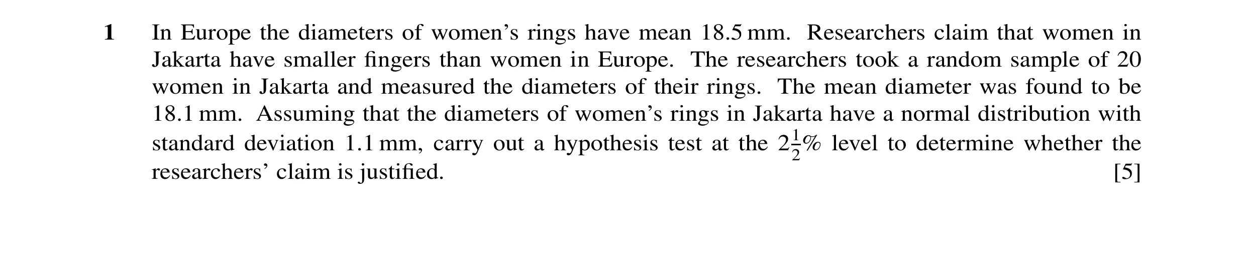
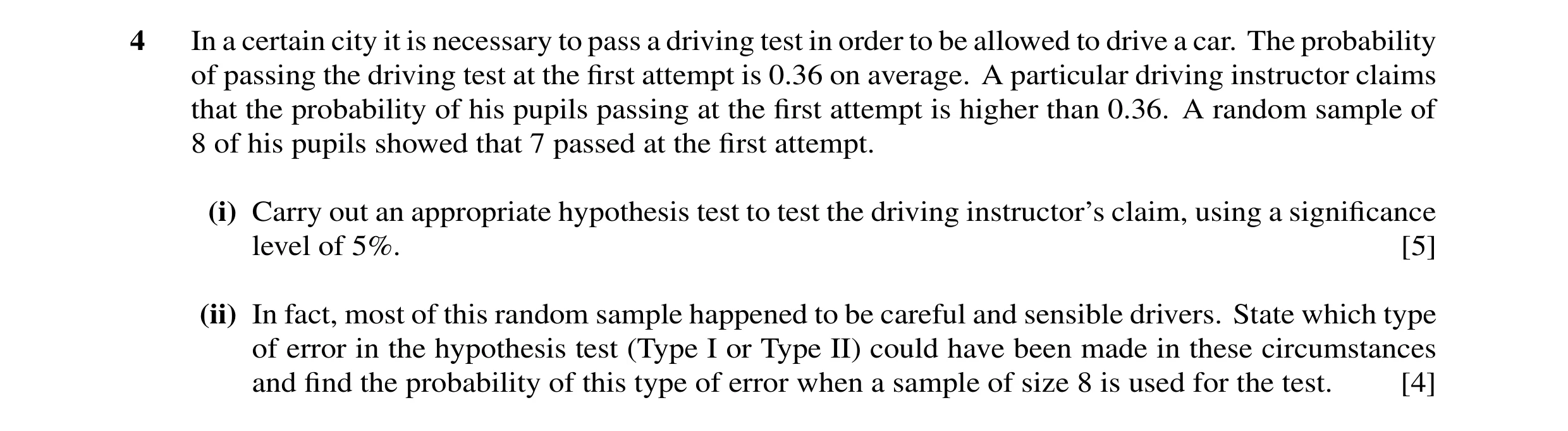
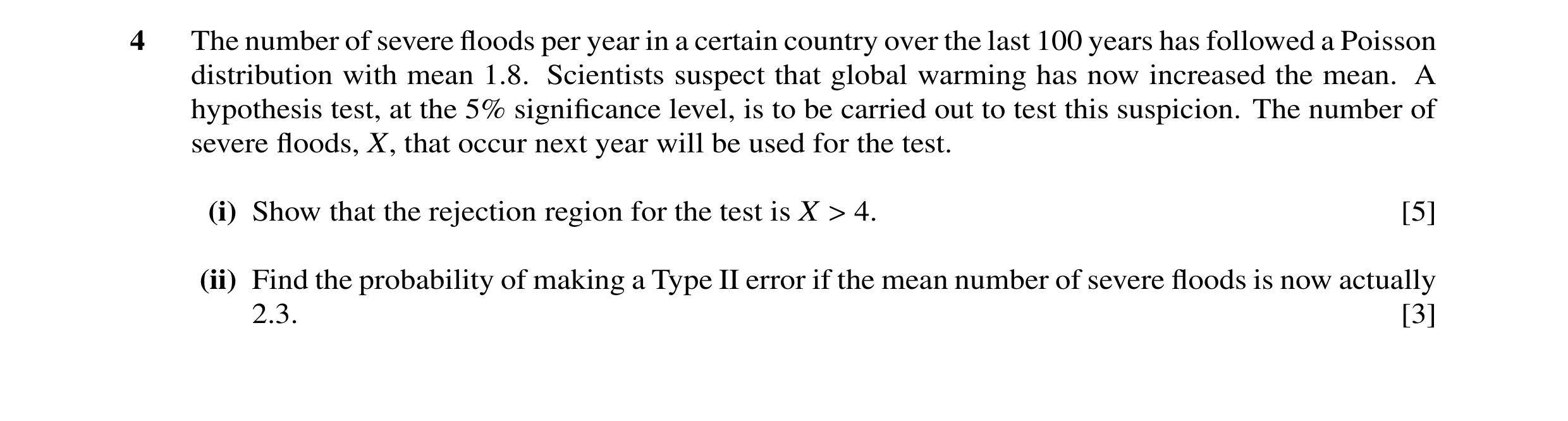 1 / 53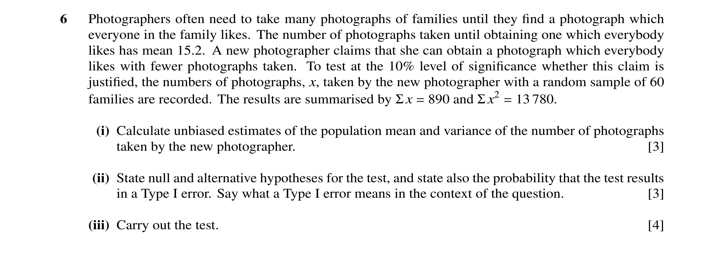
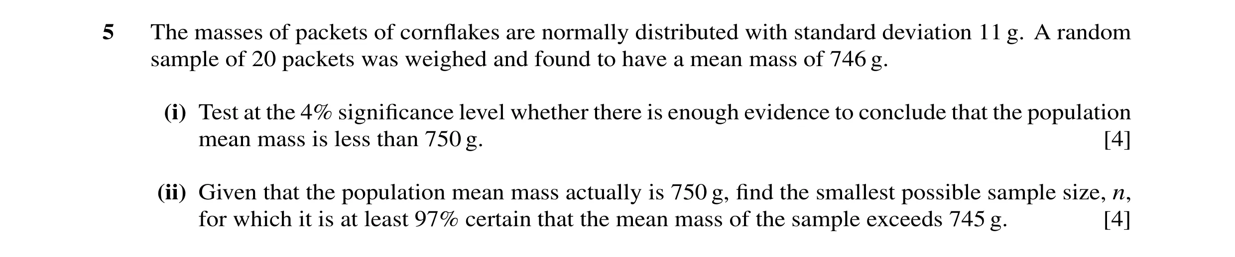
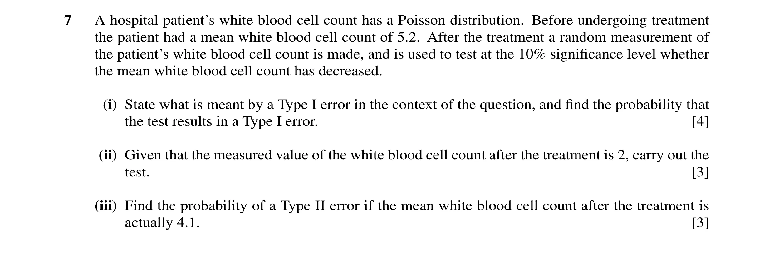
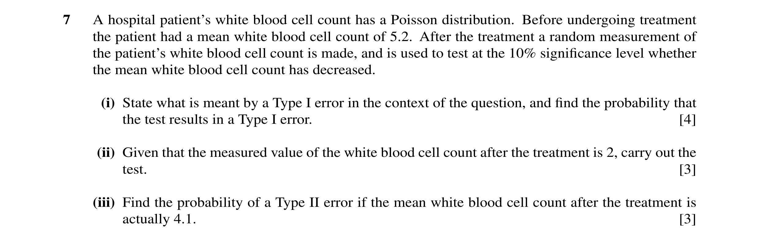 2 / 53
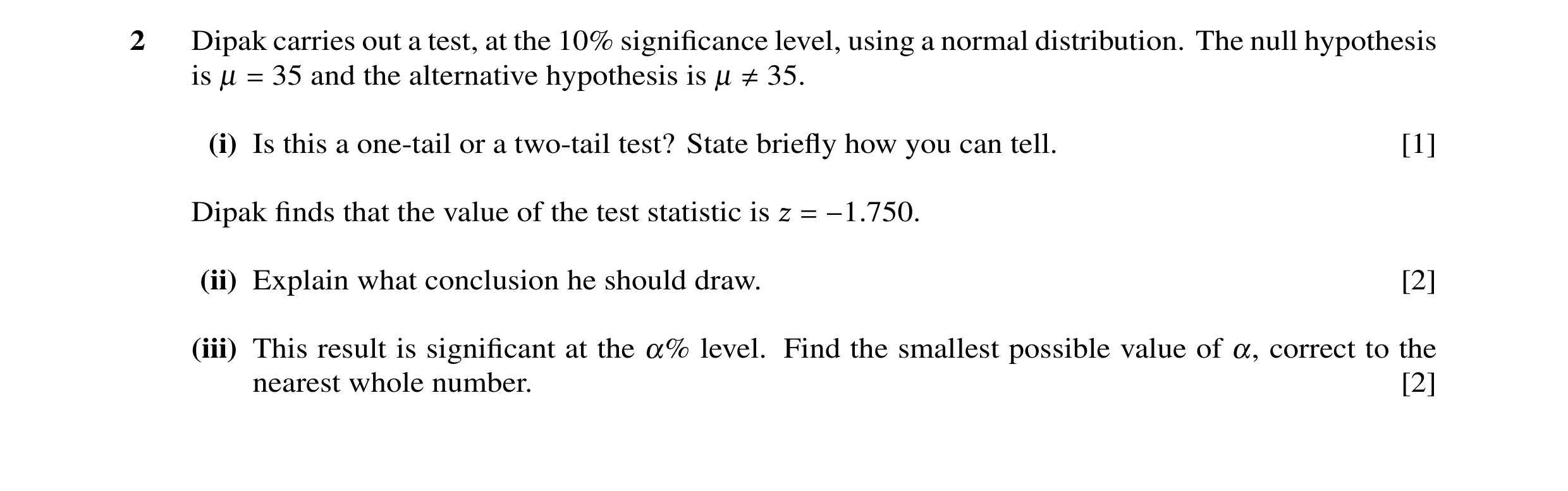
 3 / 53
 4 / 53

 5 / 53

 6 / 53

 7 / 53
 8 / 53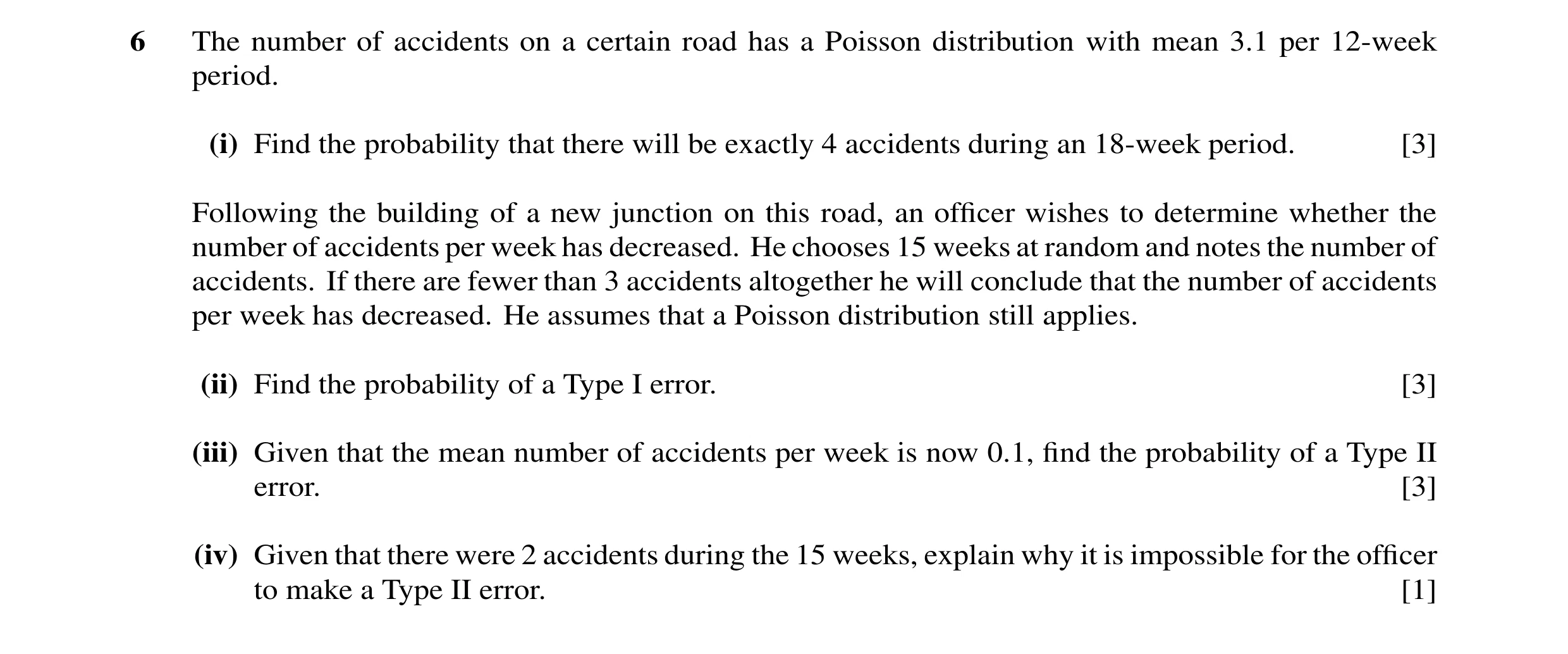
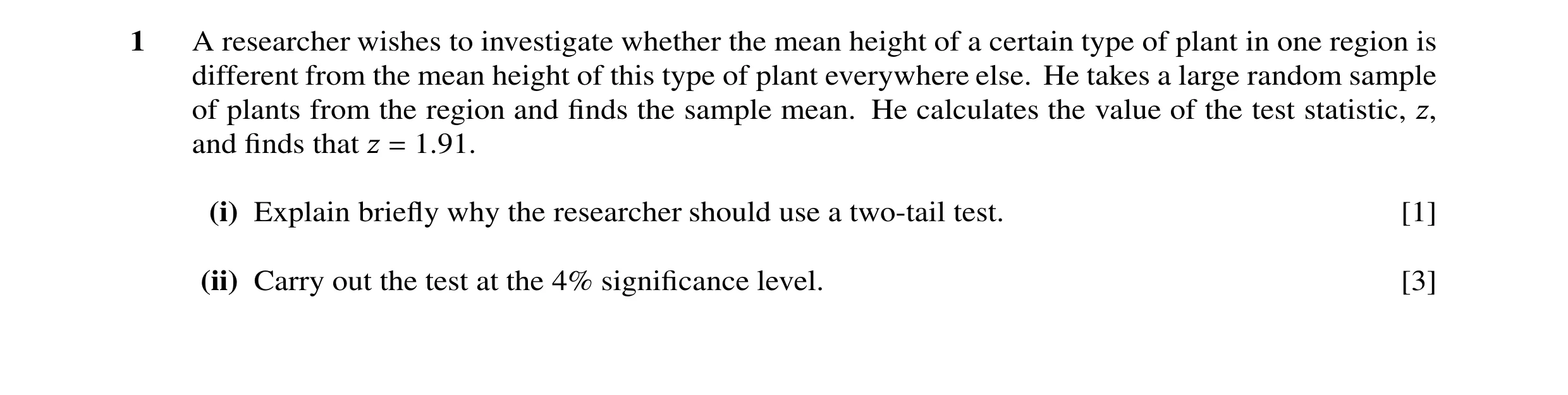
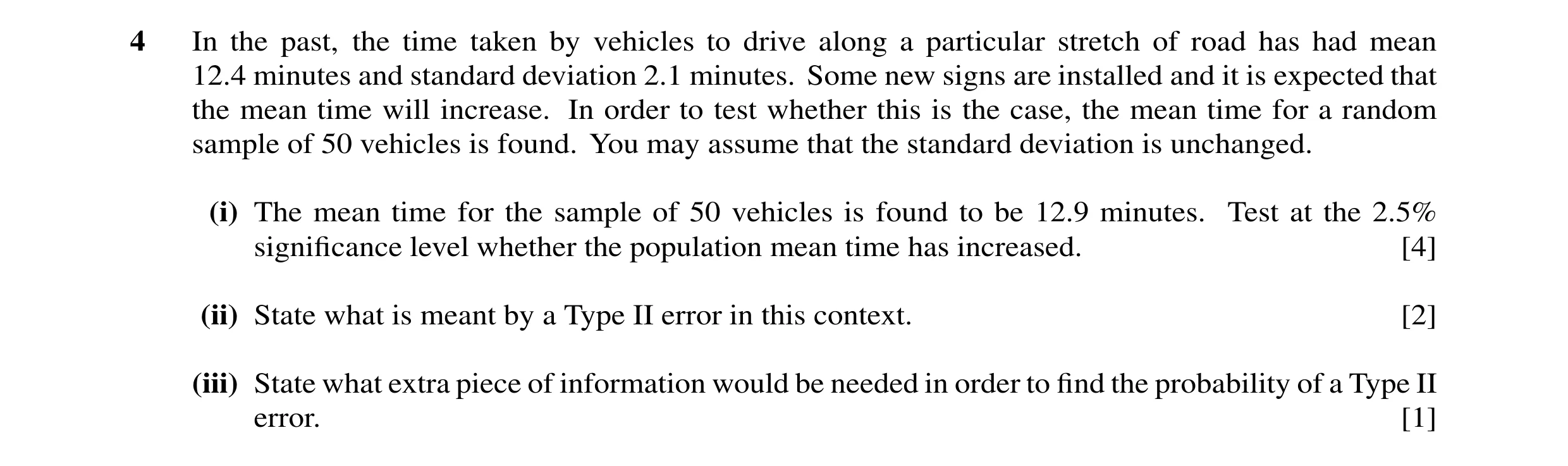
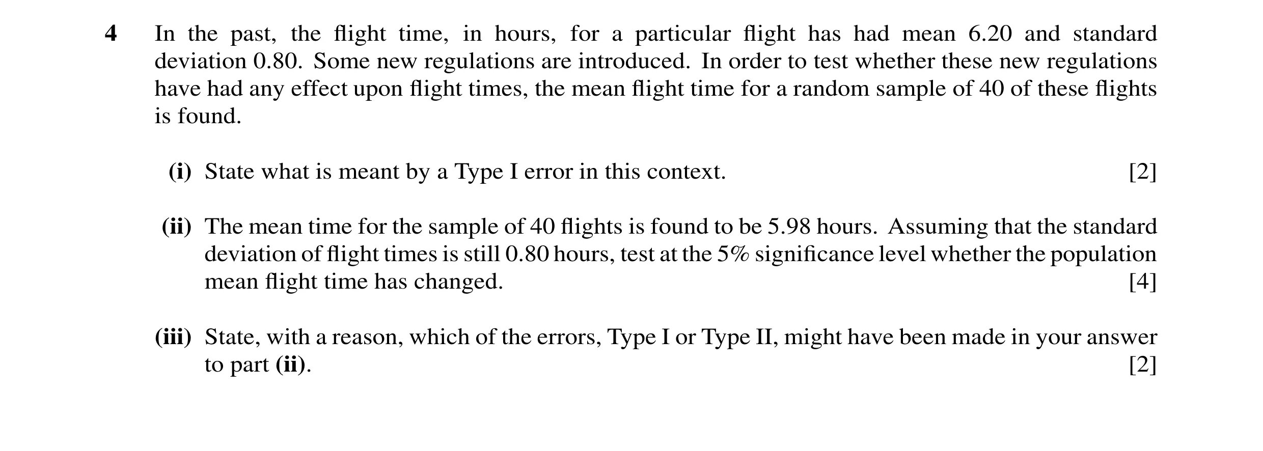 9 / 53
 10 / 53
 11 / 53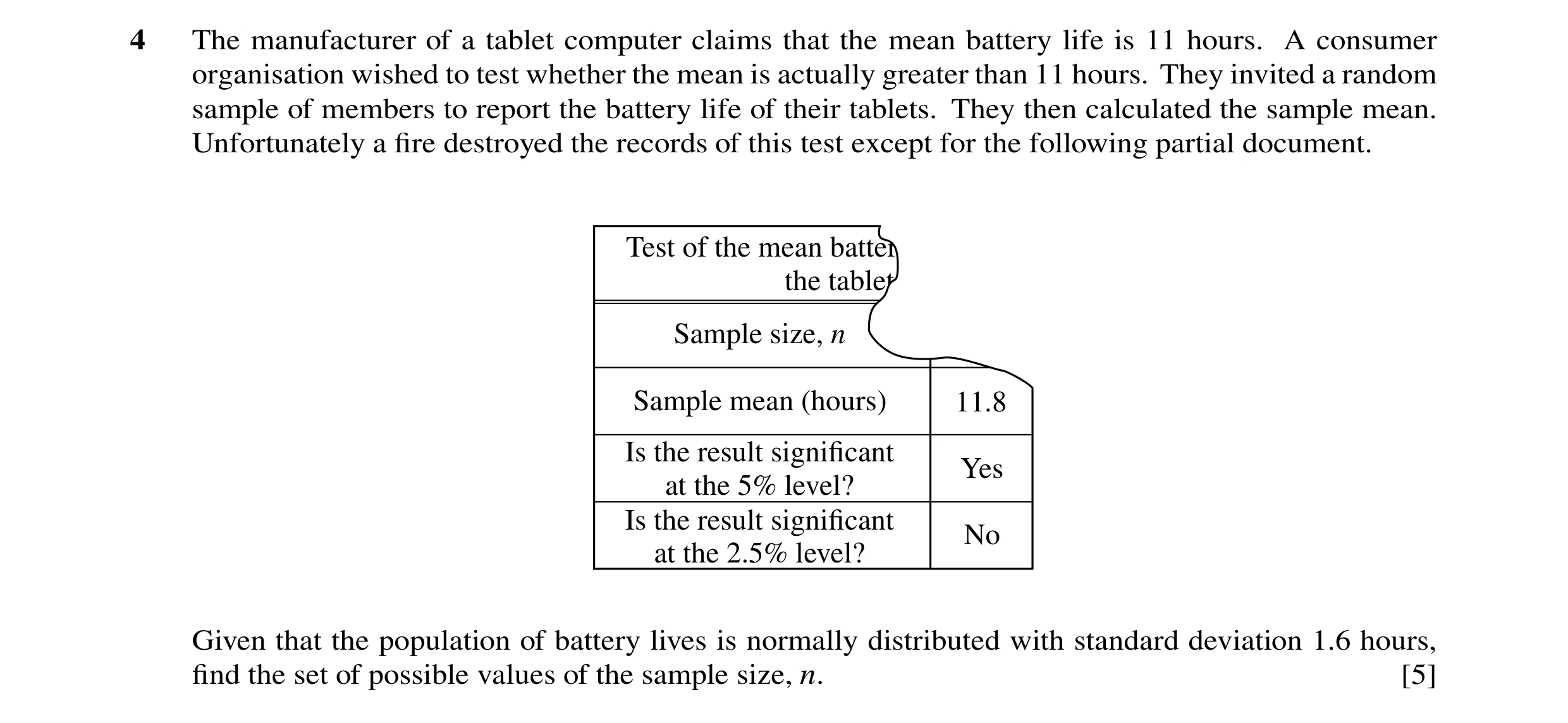
 12 / 53
 13 / 53
 14 / 53
 15 / 53
 18 / 53
 19 / 53
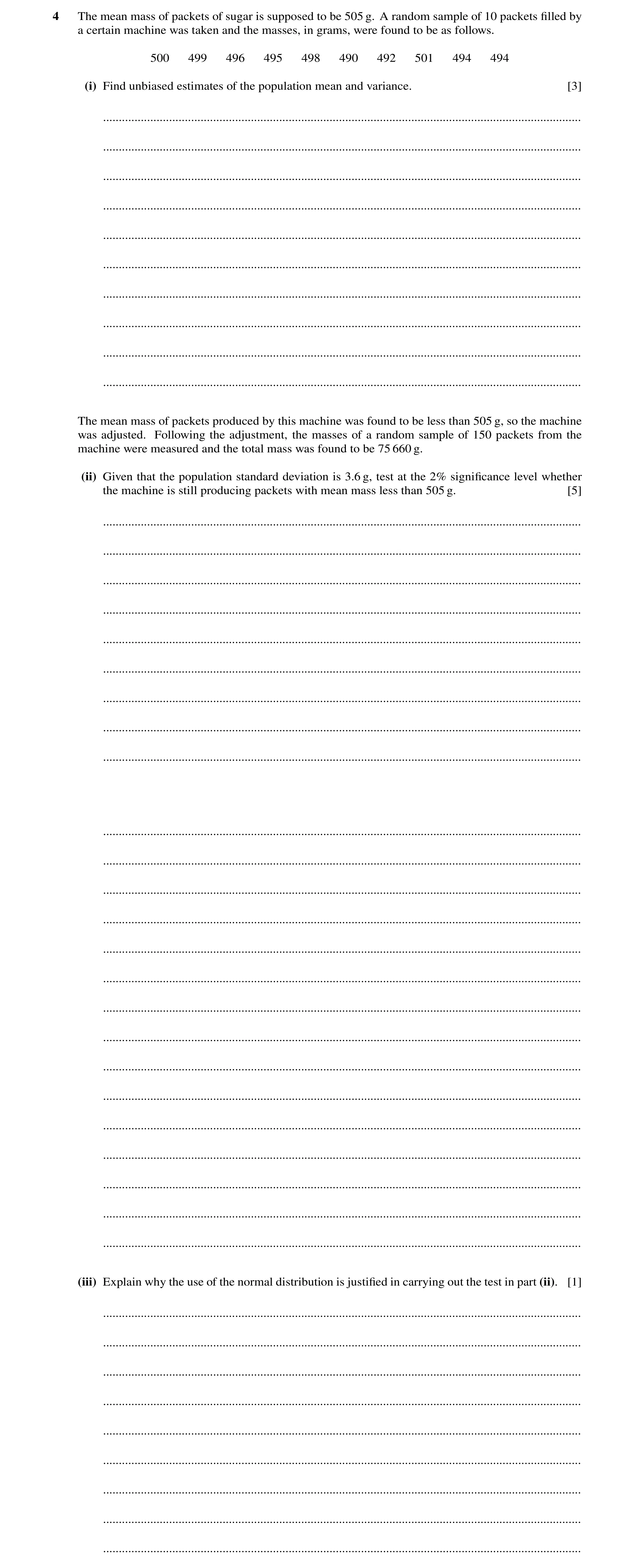


 40 / 53
 5
5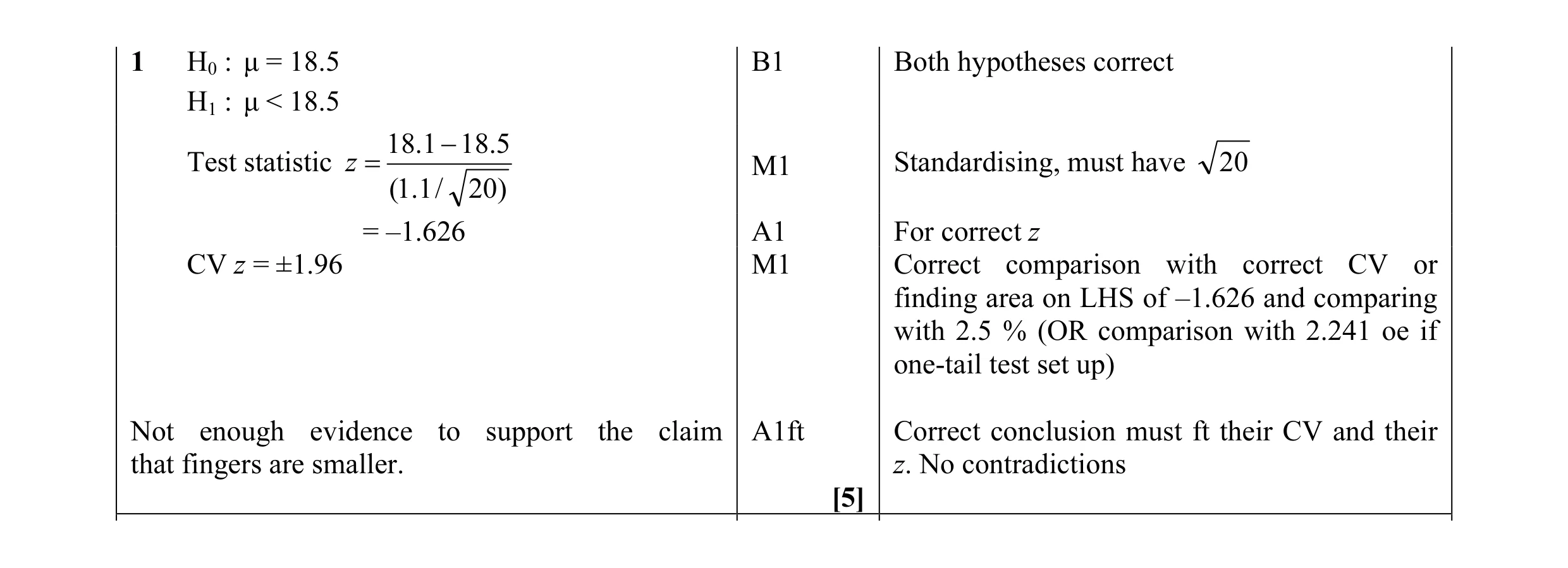 5
5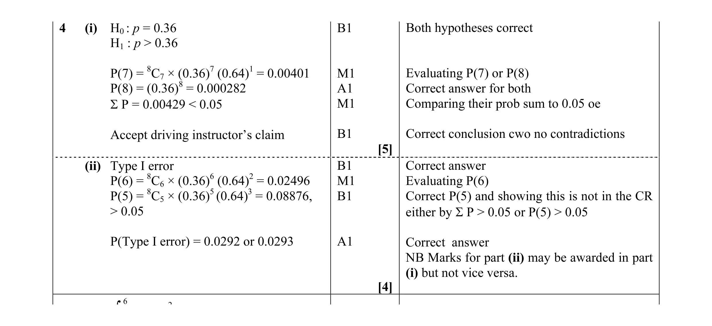 9
9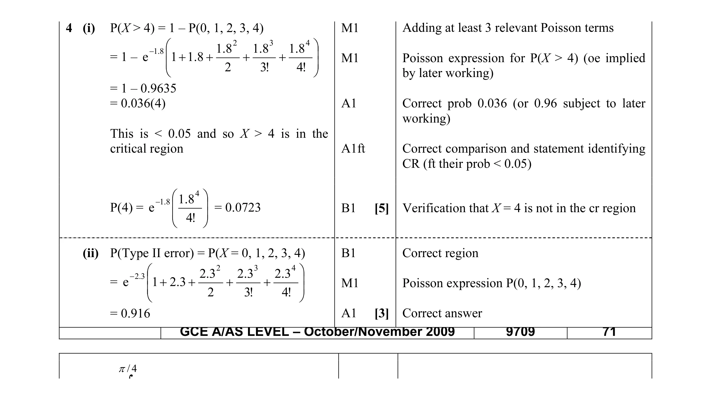 8
8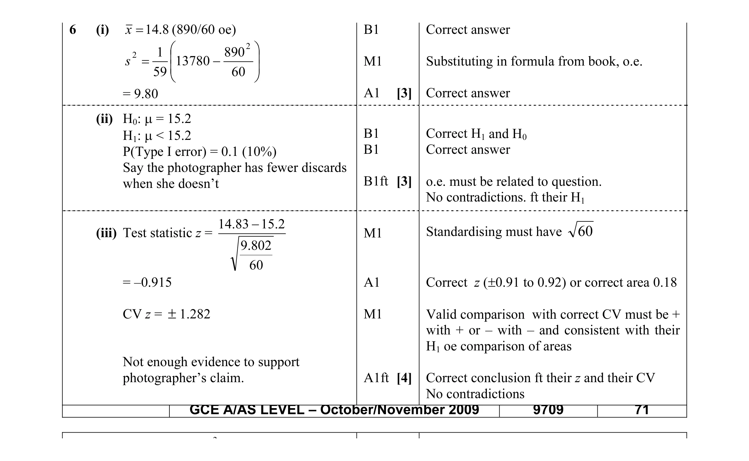 10
10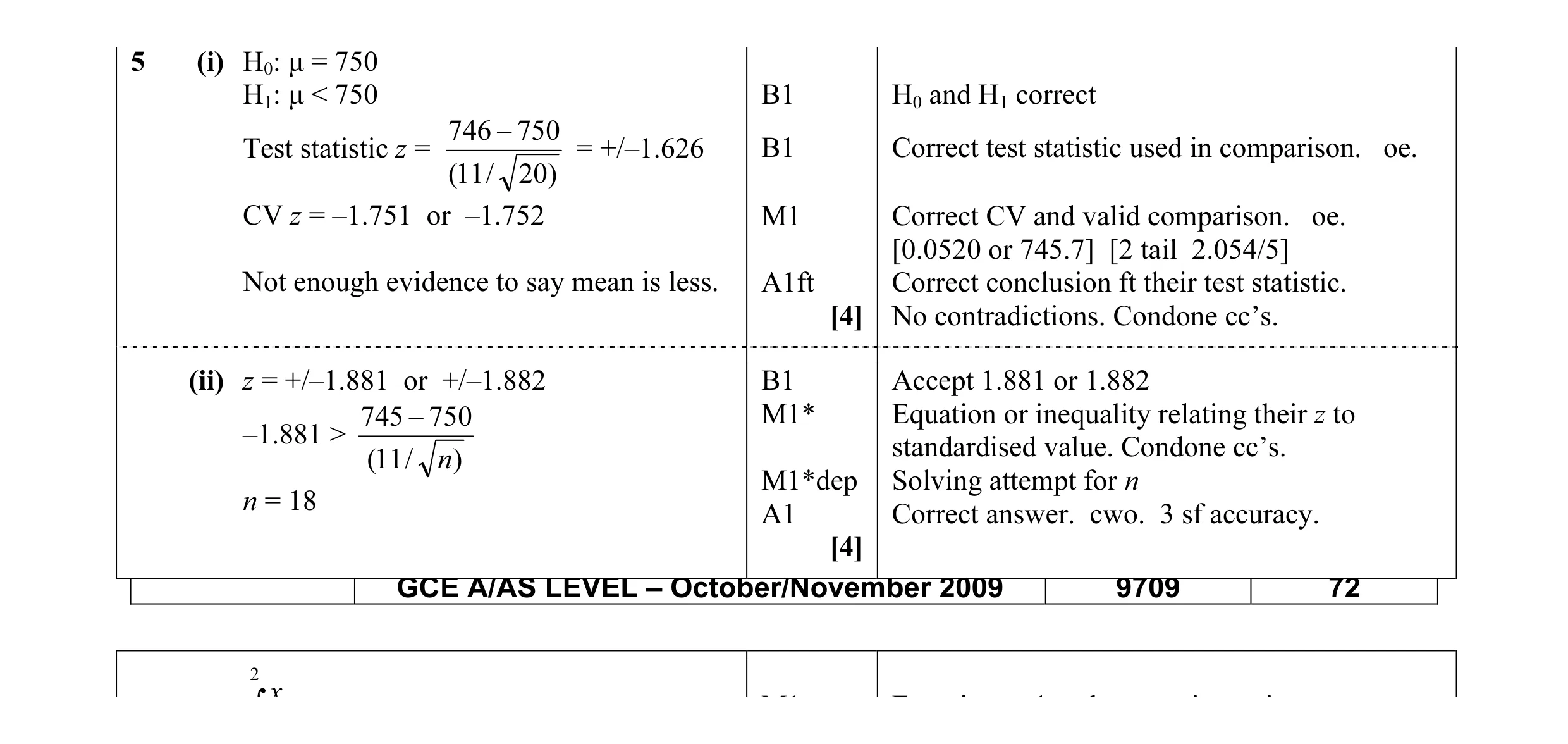 8
8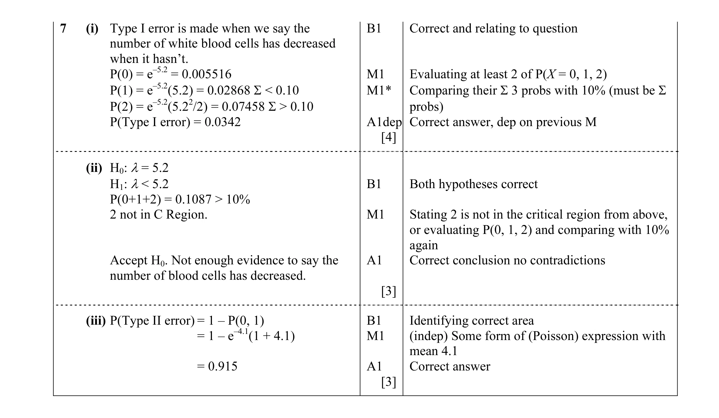 10
10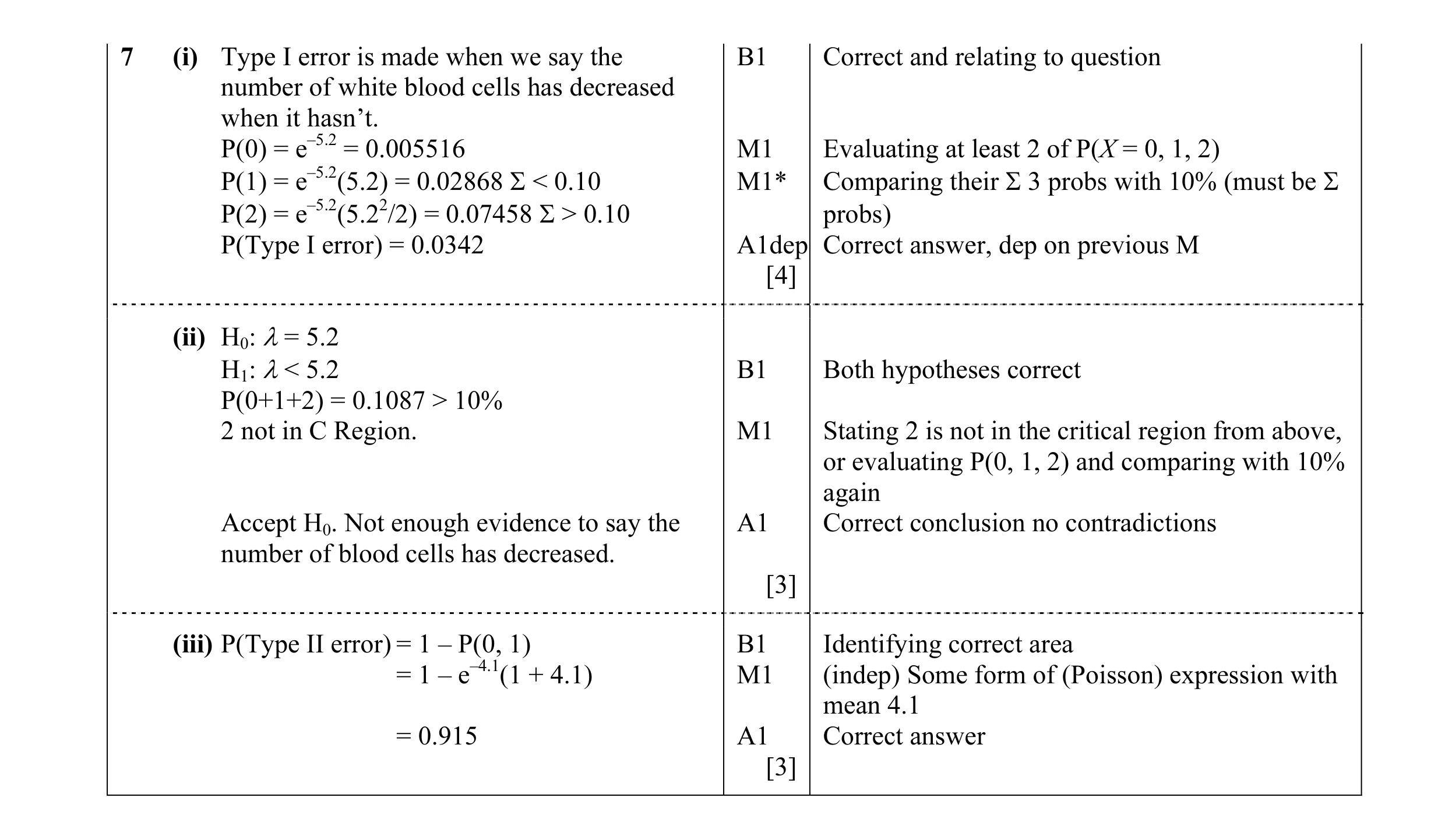 10
10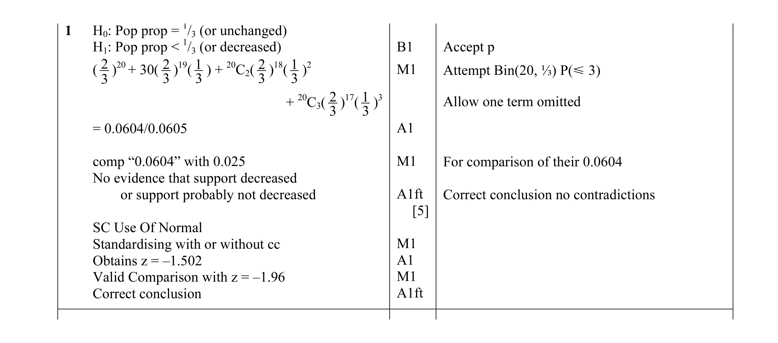 5
5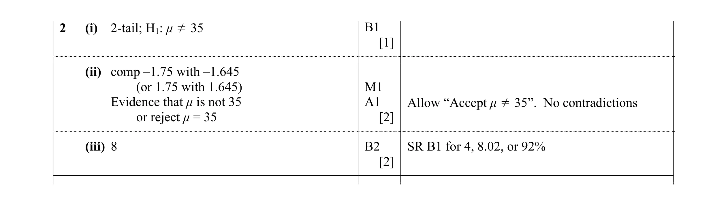 5
5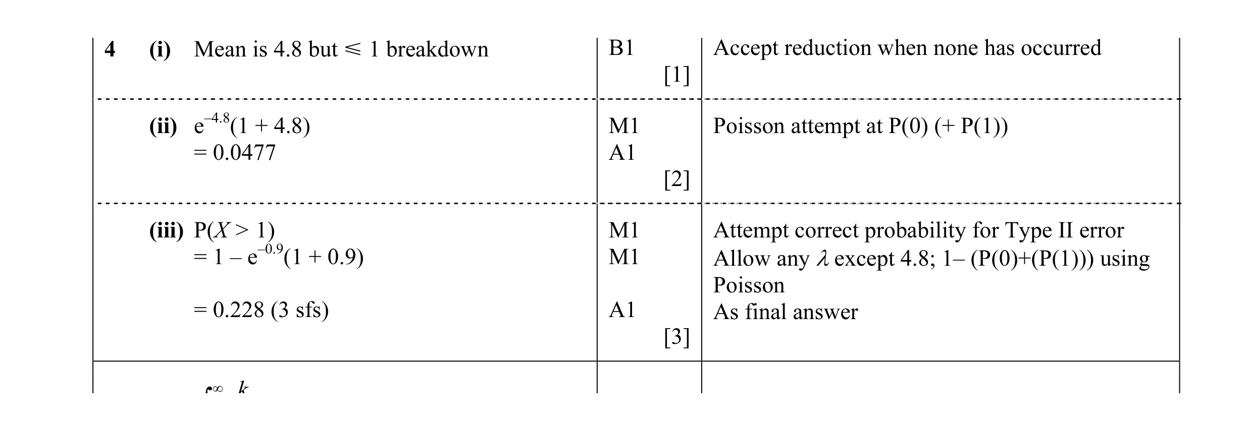 6
6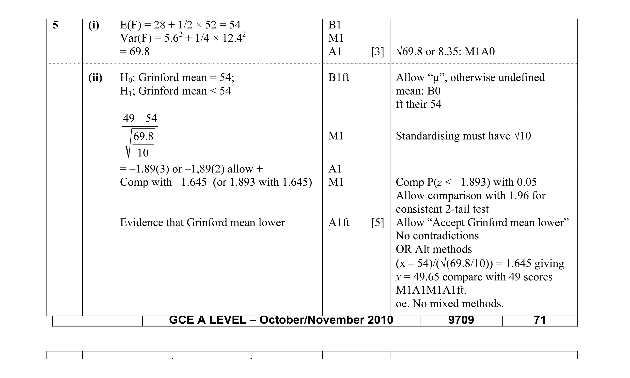 8
8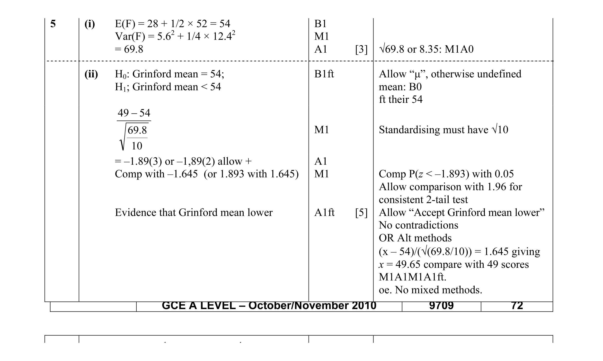 8
8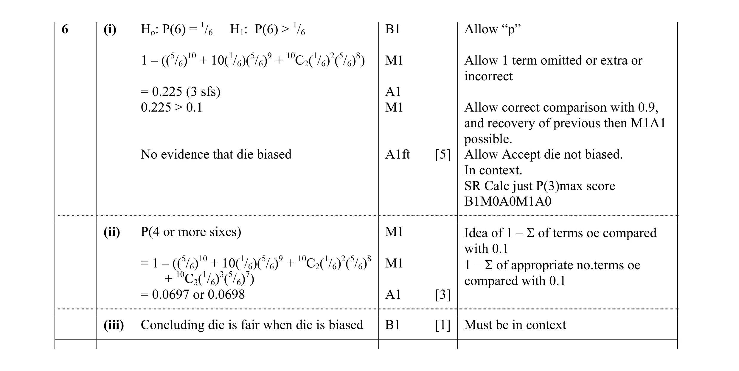 9
9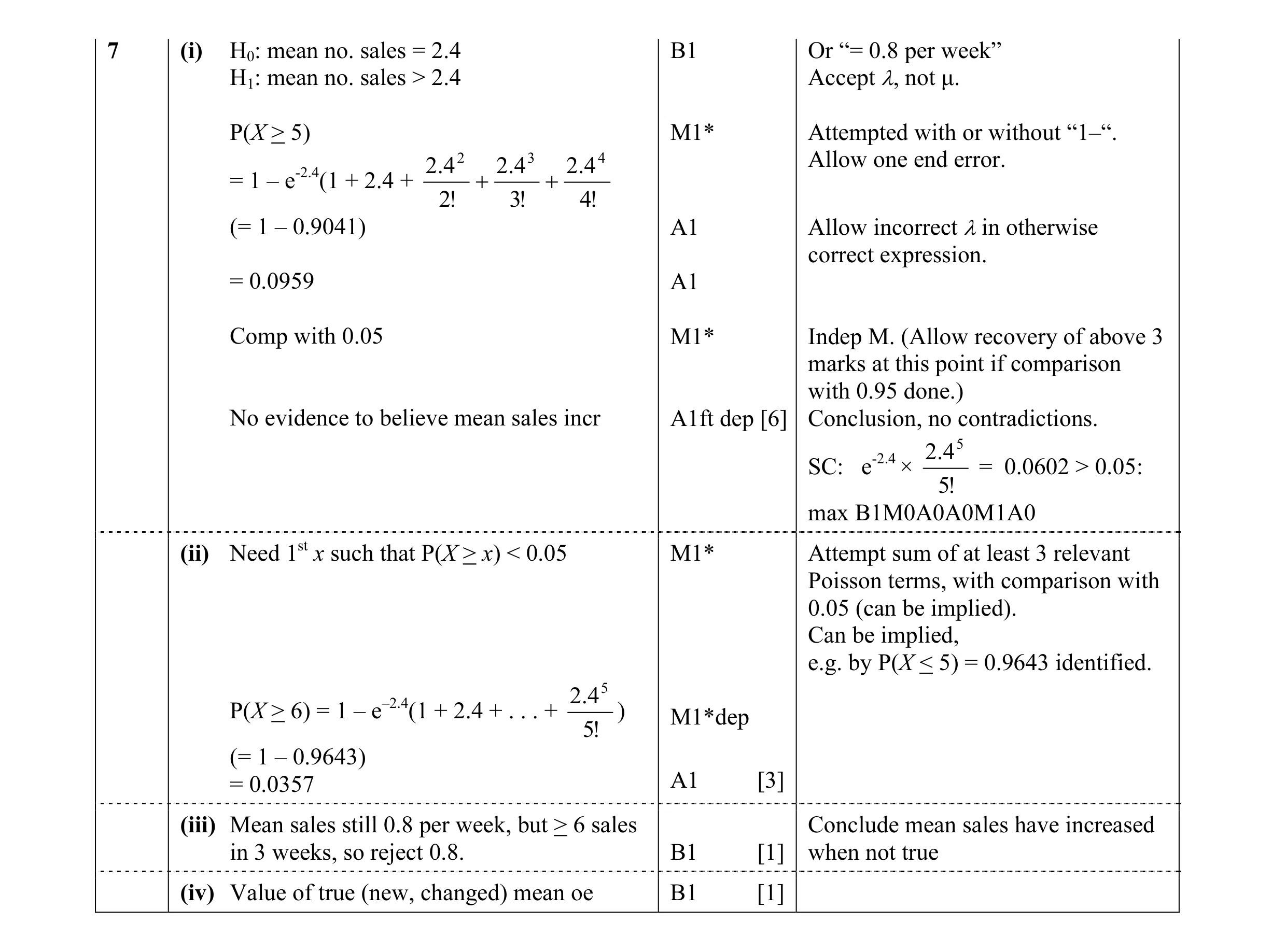 11
11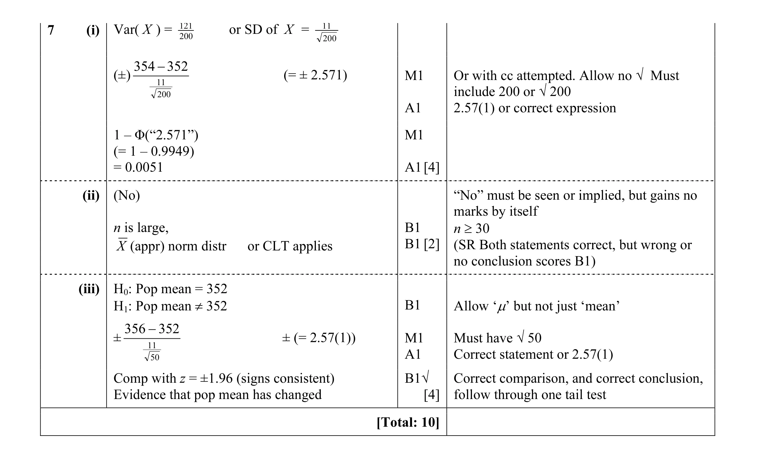 10
10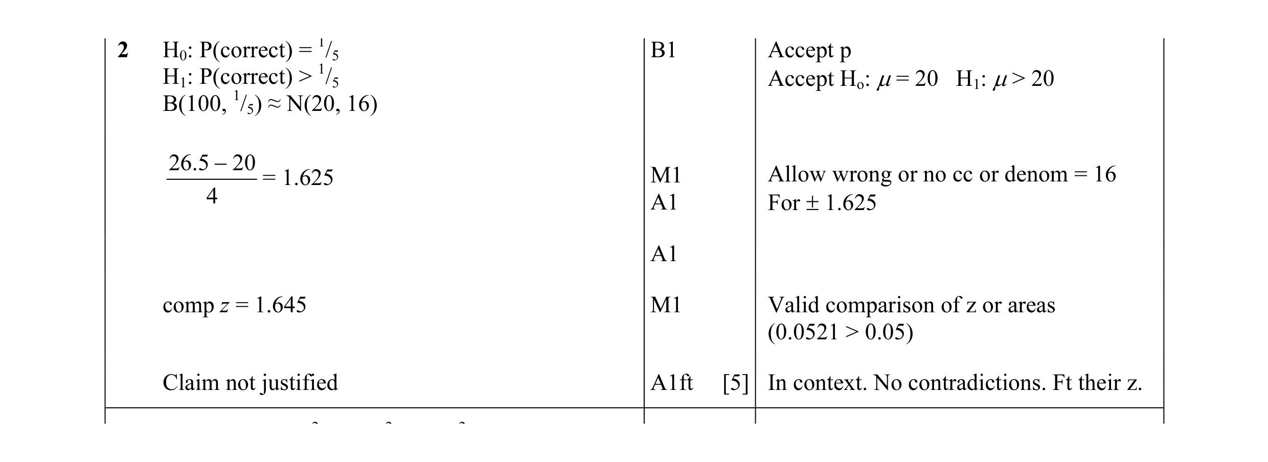 5
5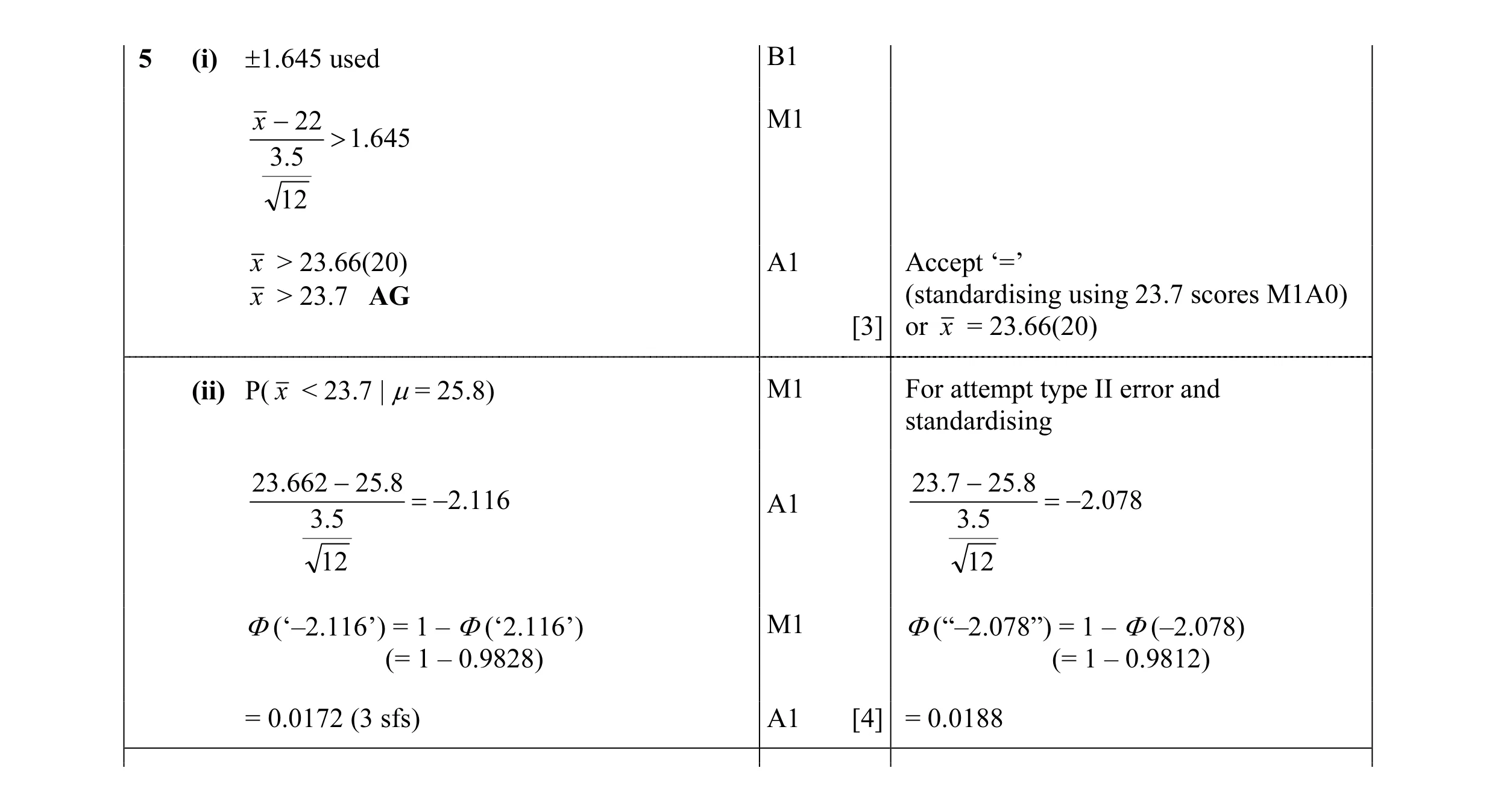 7
7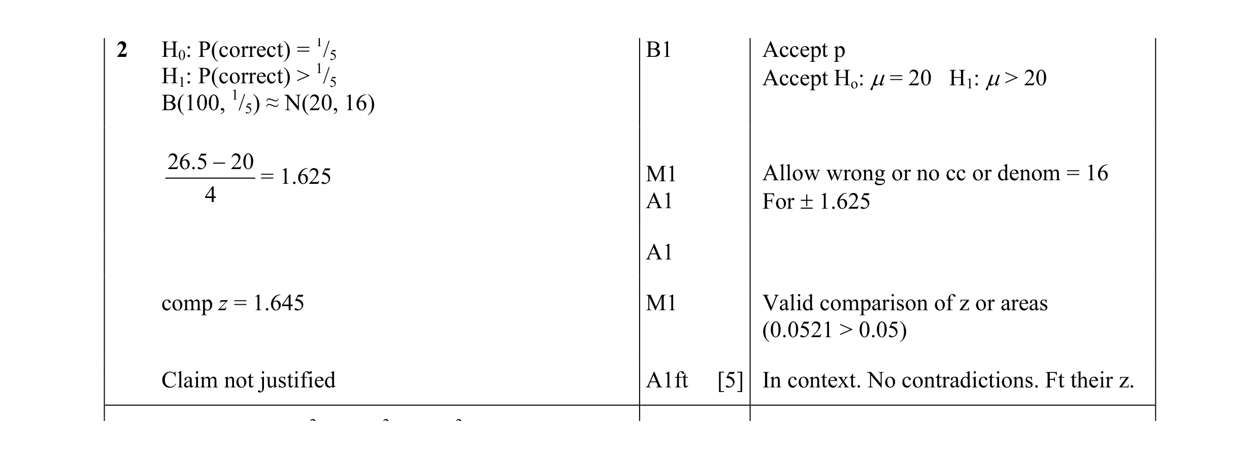 5
5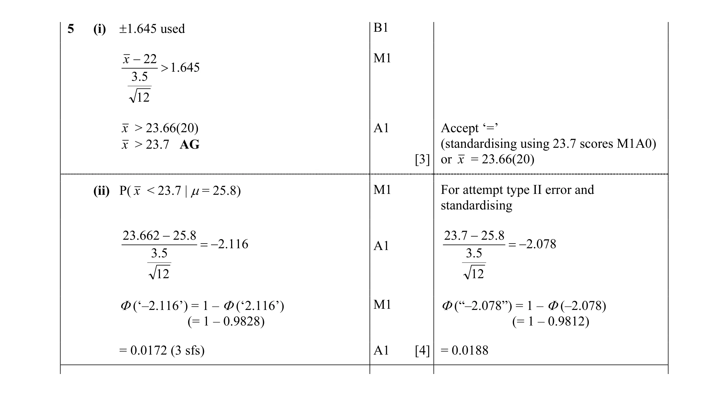 7
7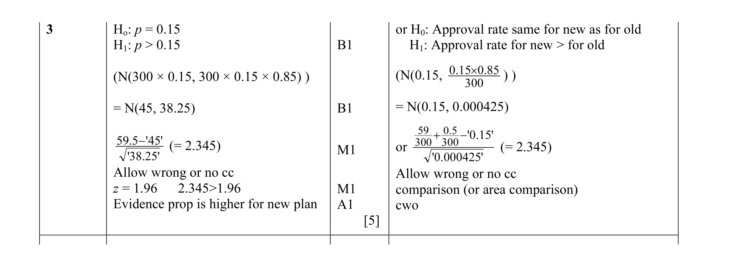 5
5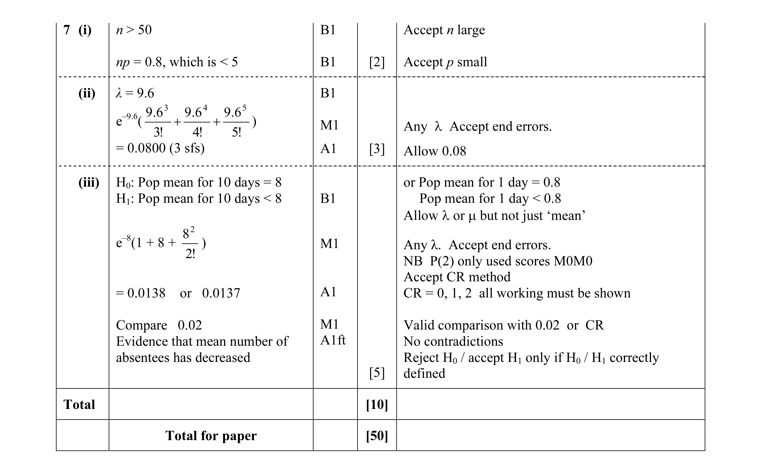 10
10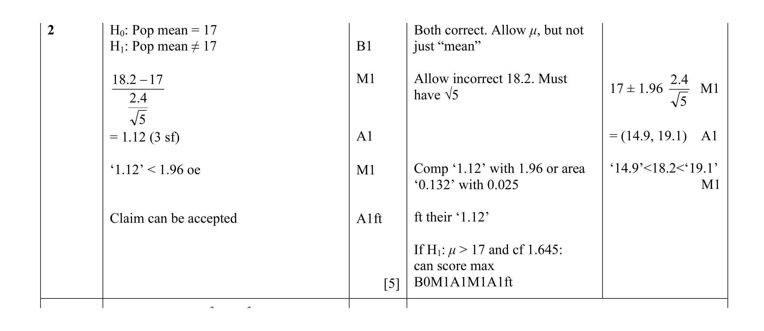 5
5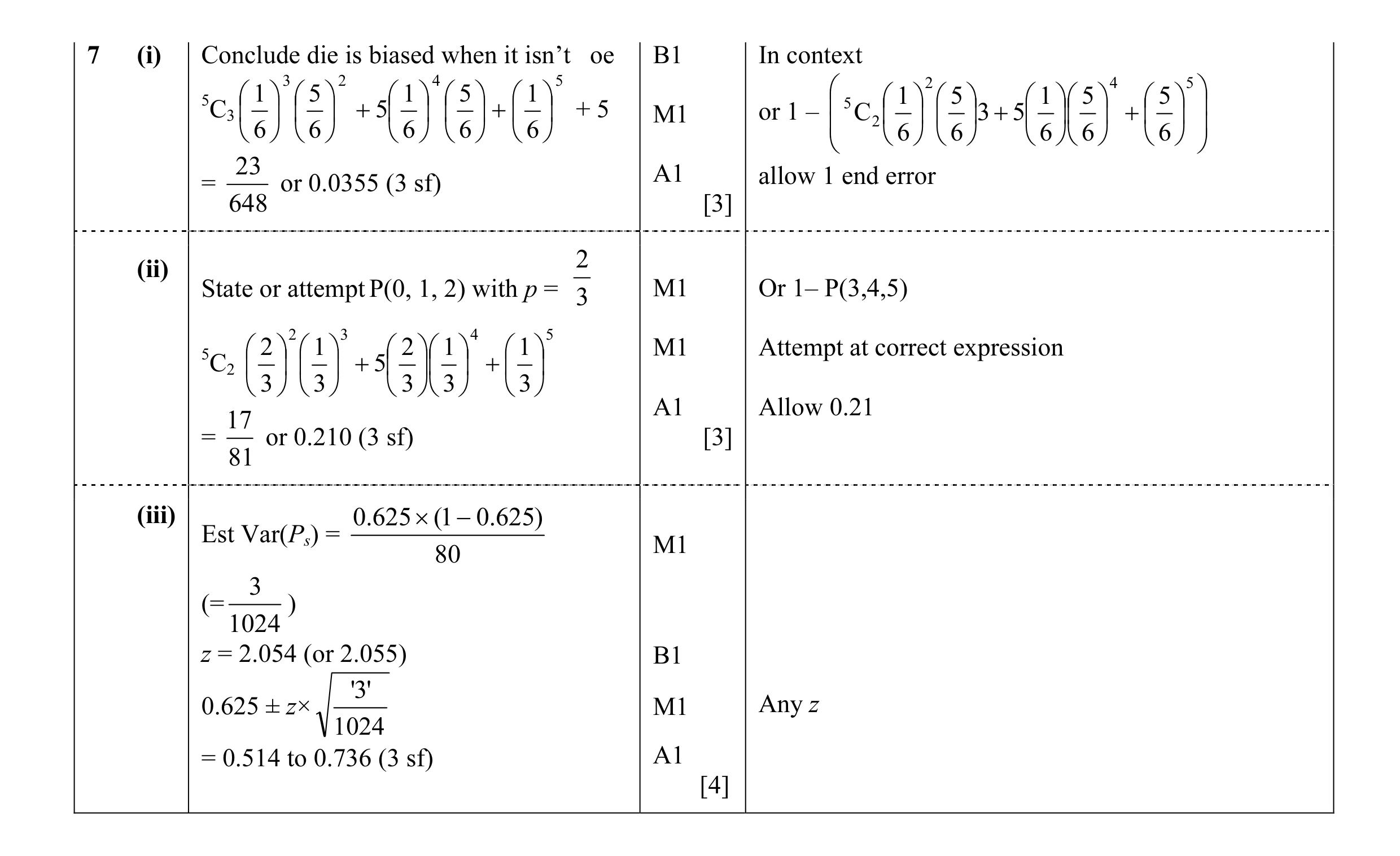 10
10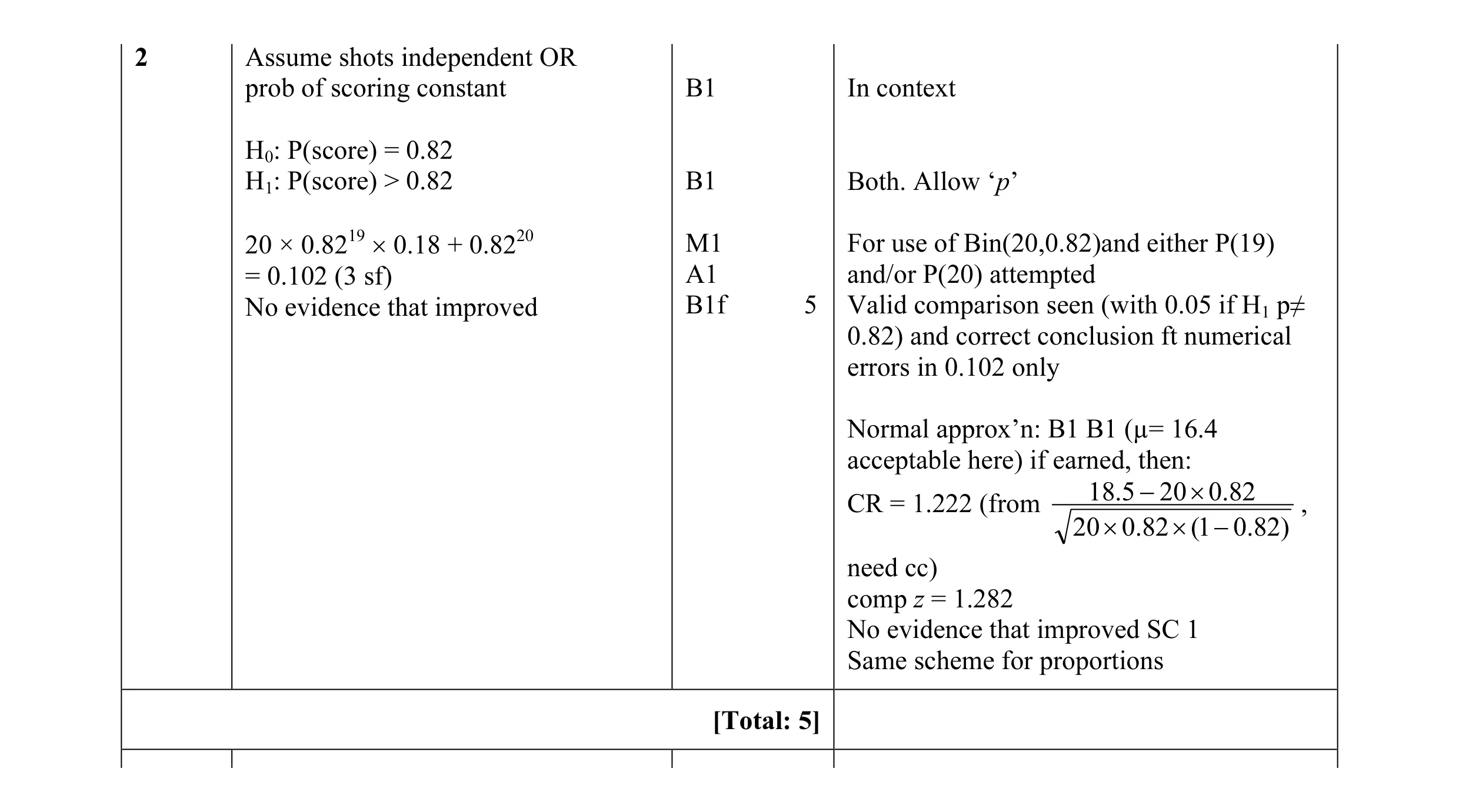 5
5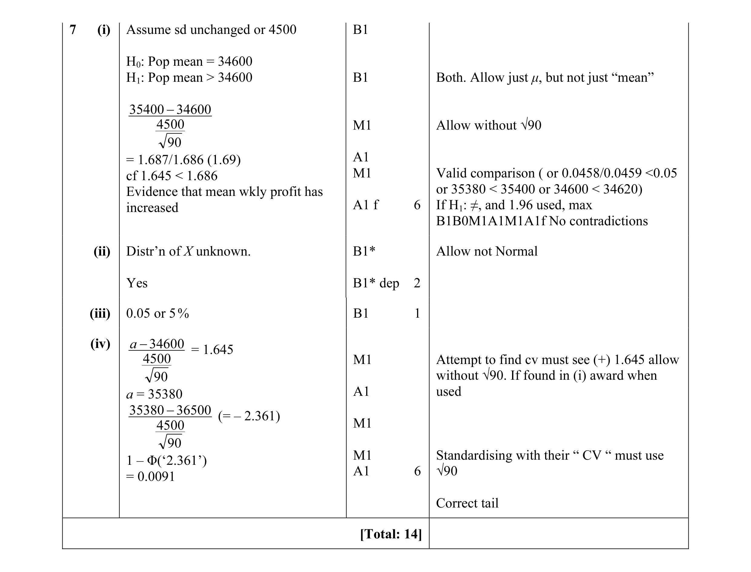 14
14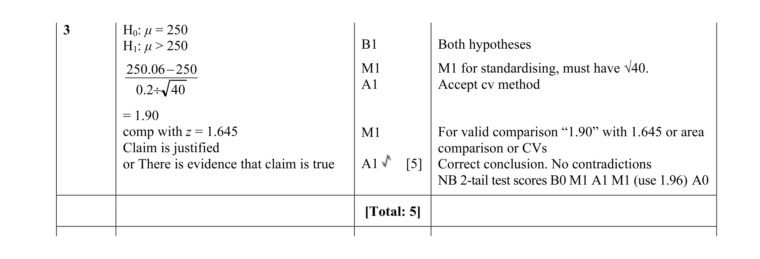 5
5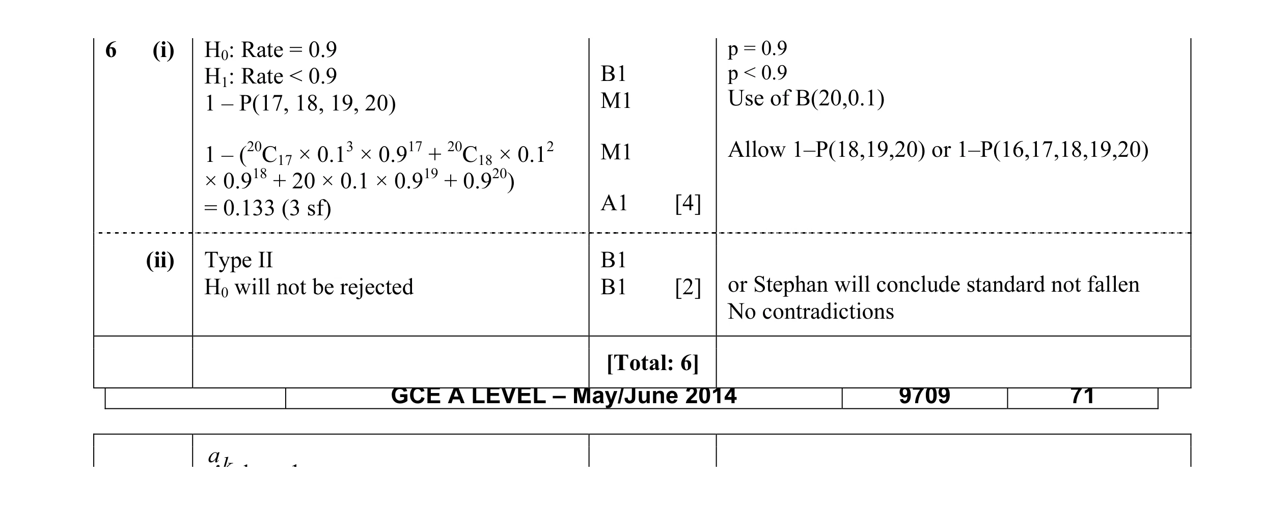 6
6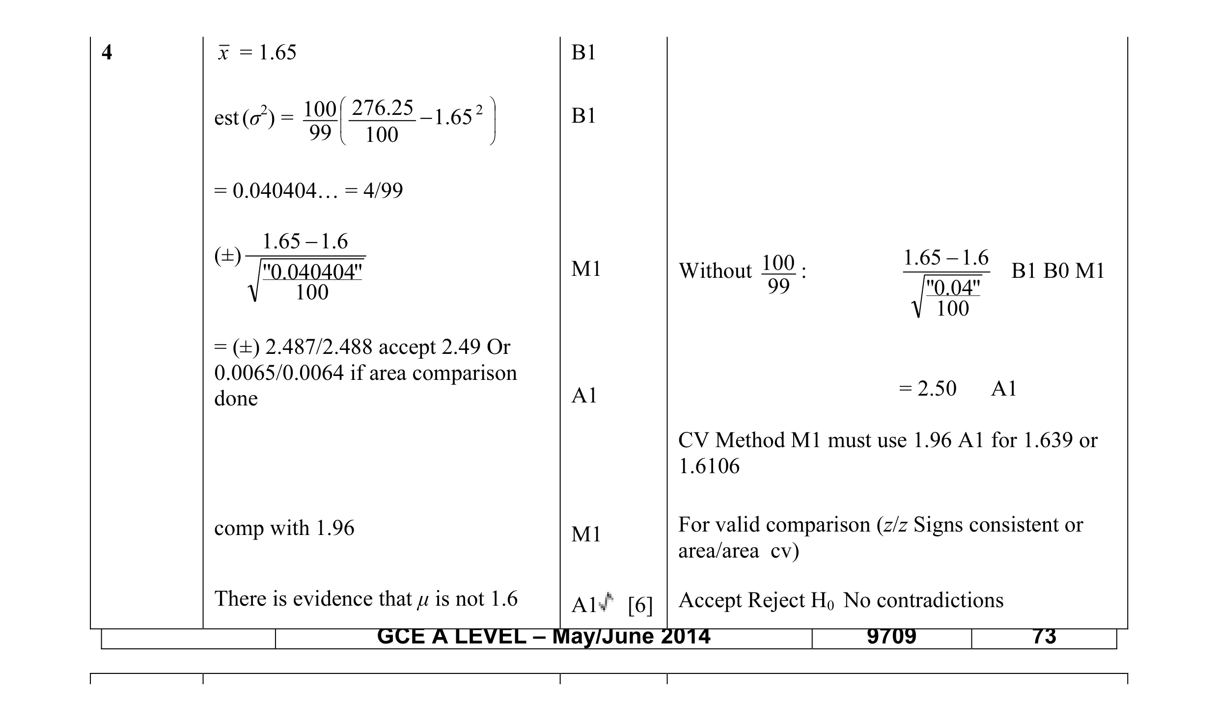 6
6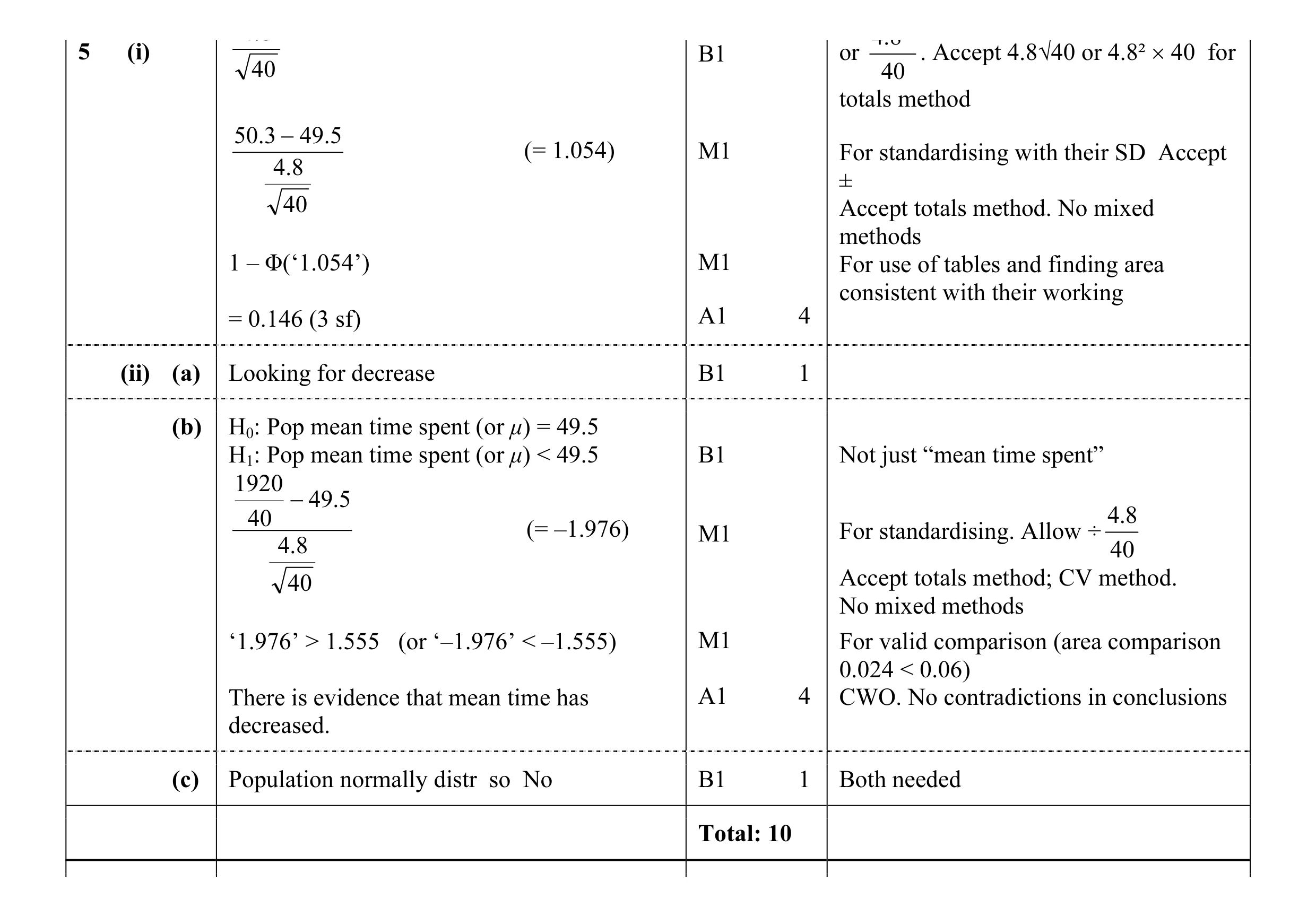 10
10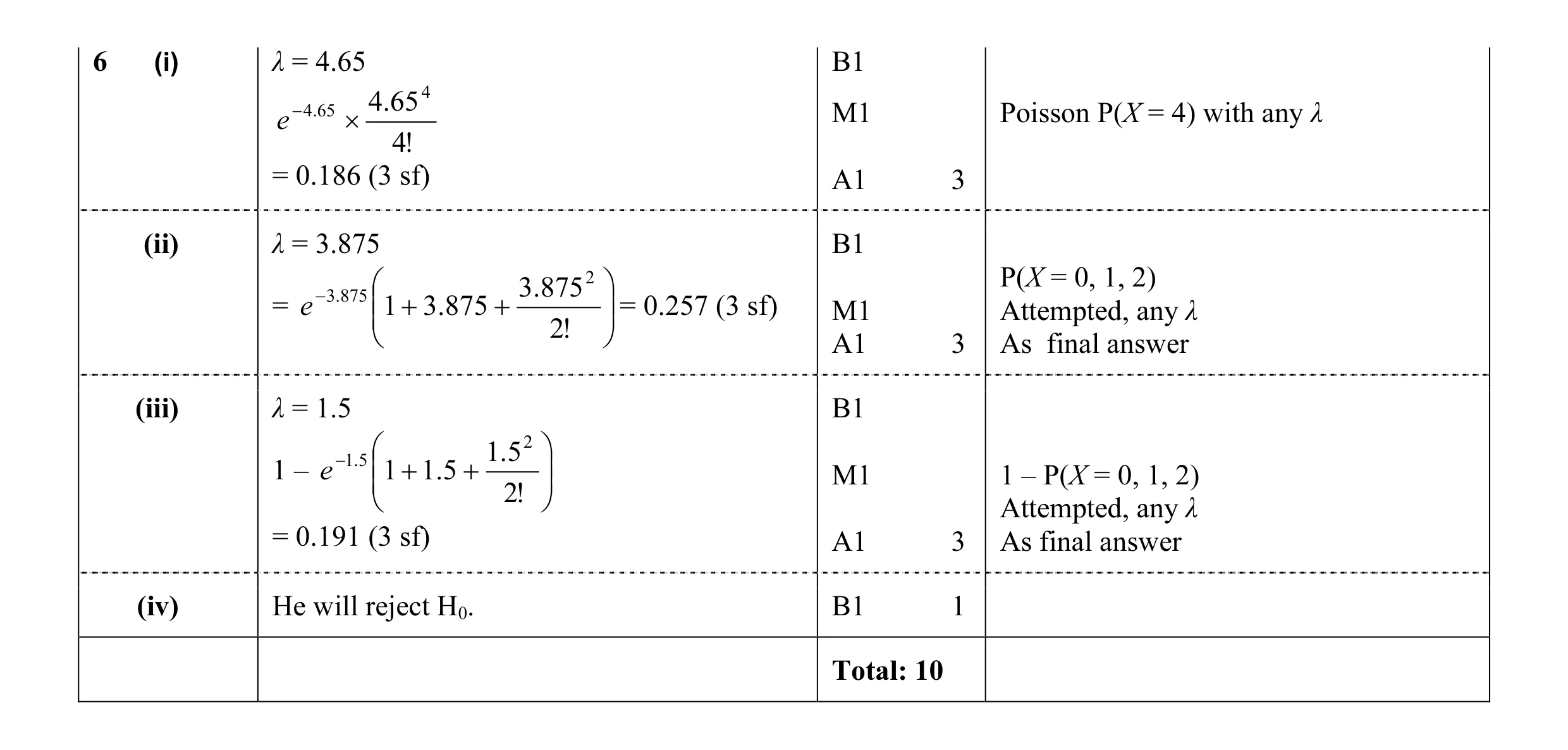 10
10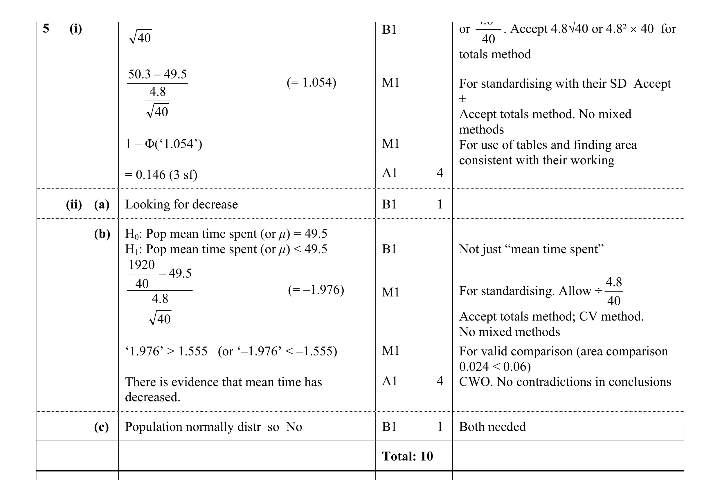 10
10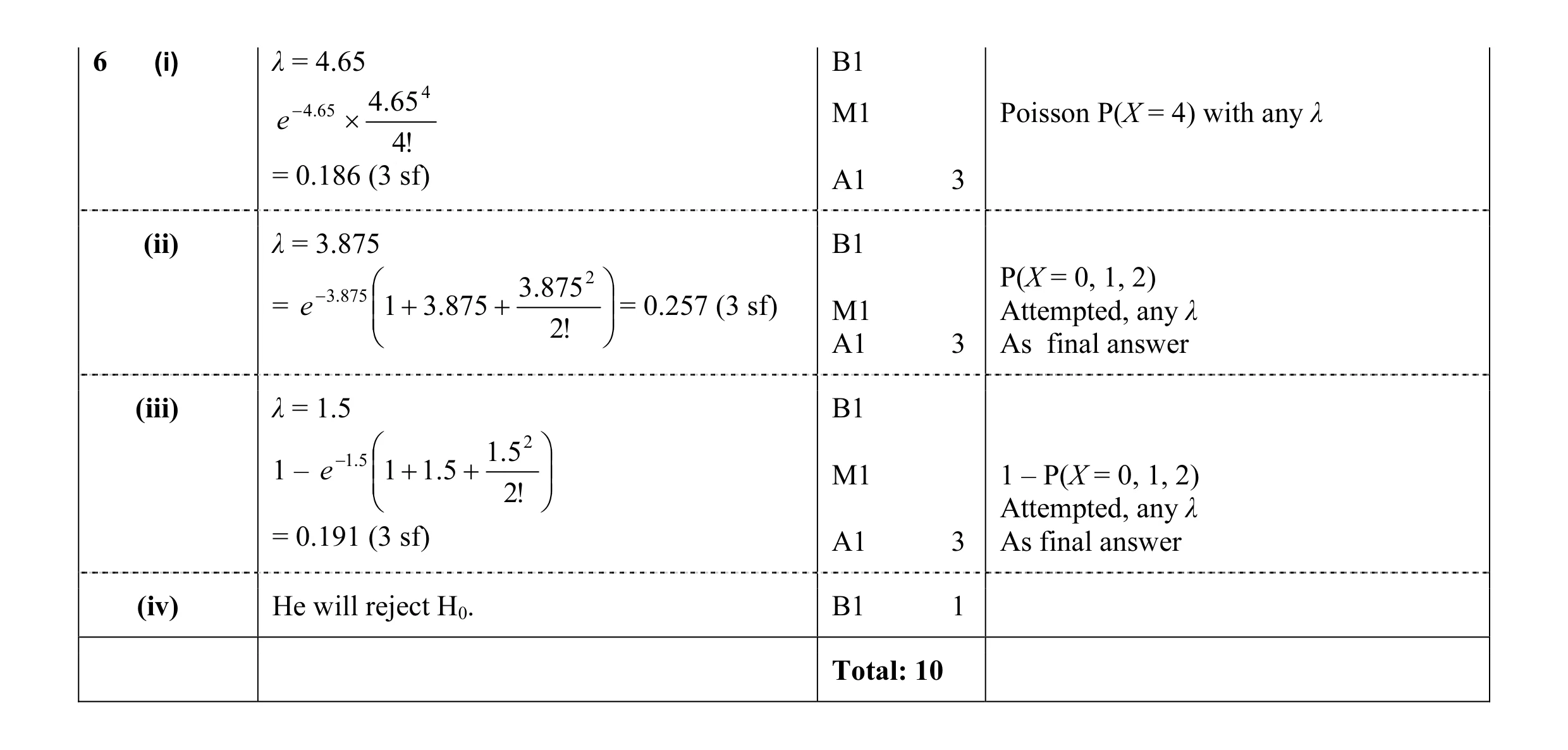 10
10 4
4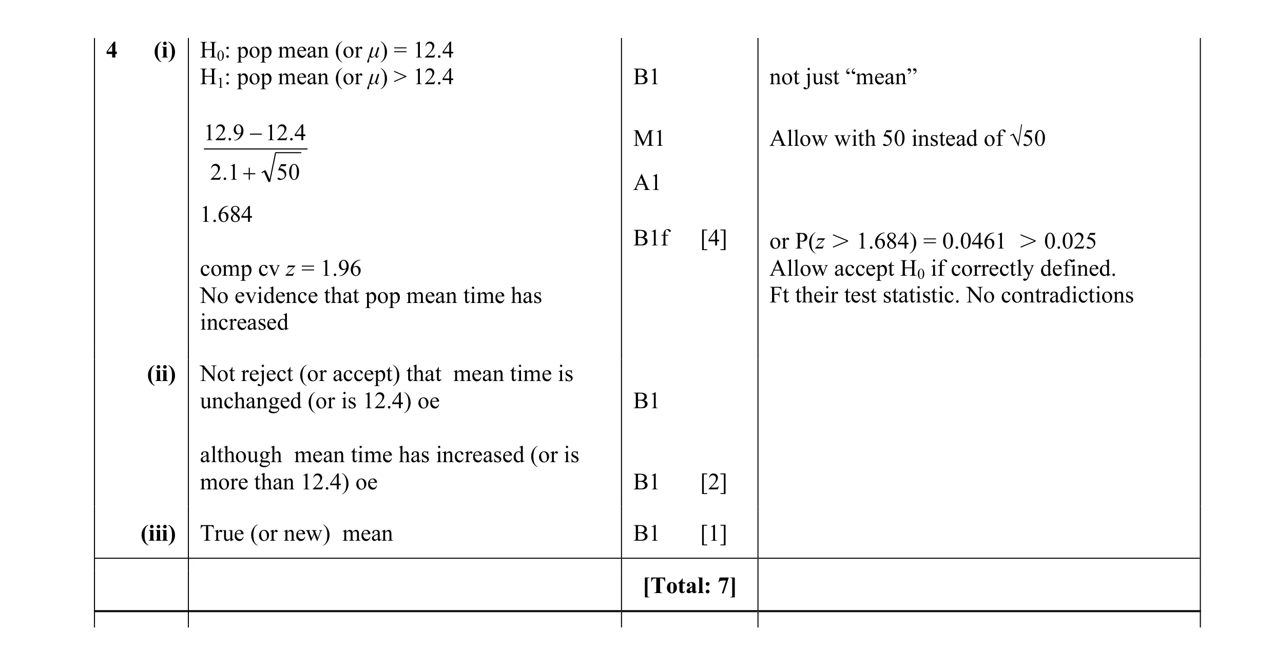 7
7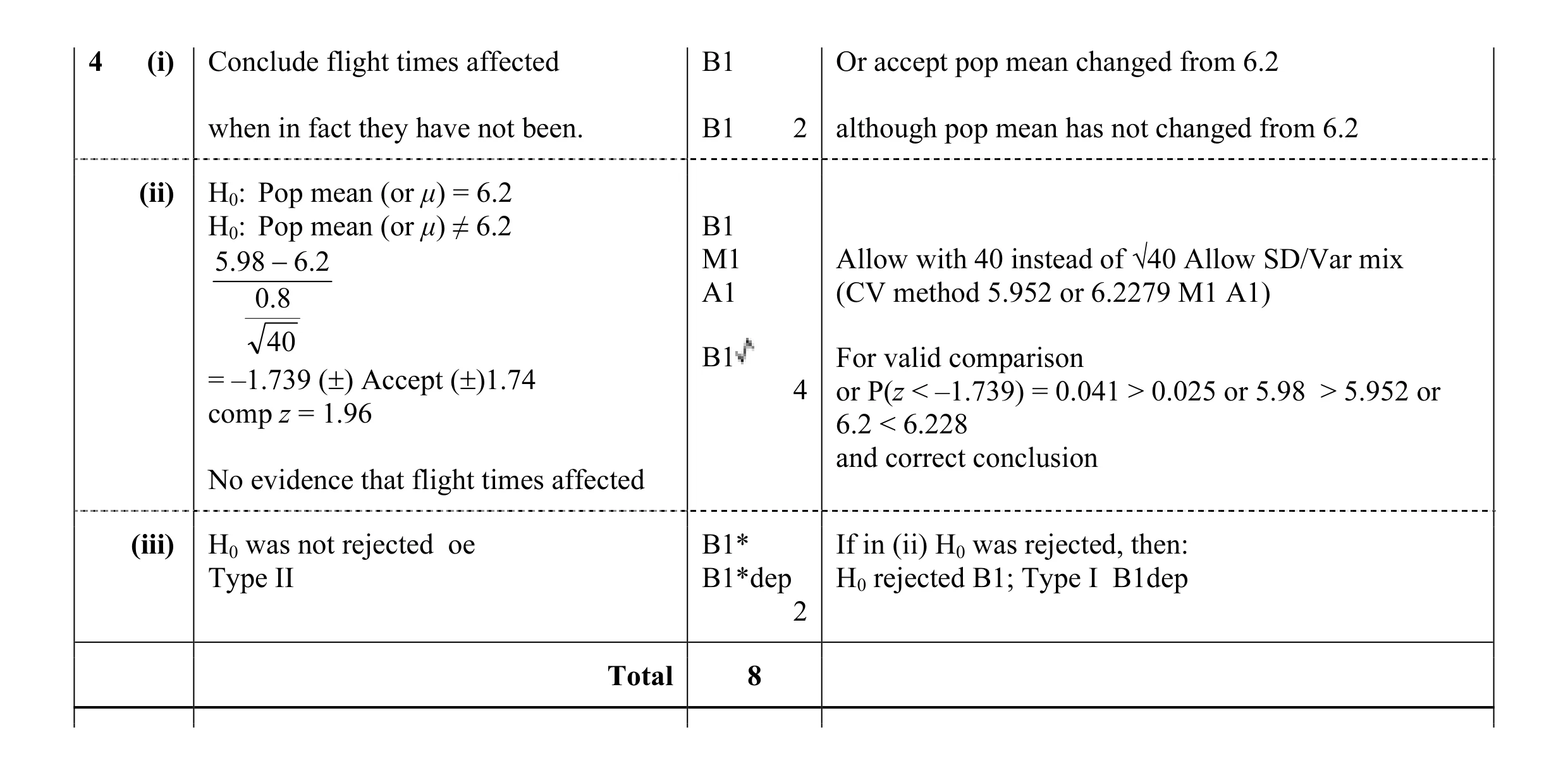 8
8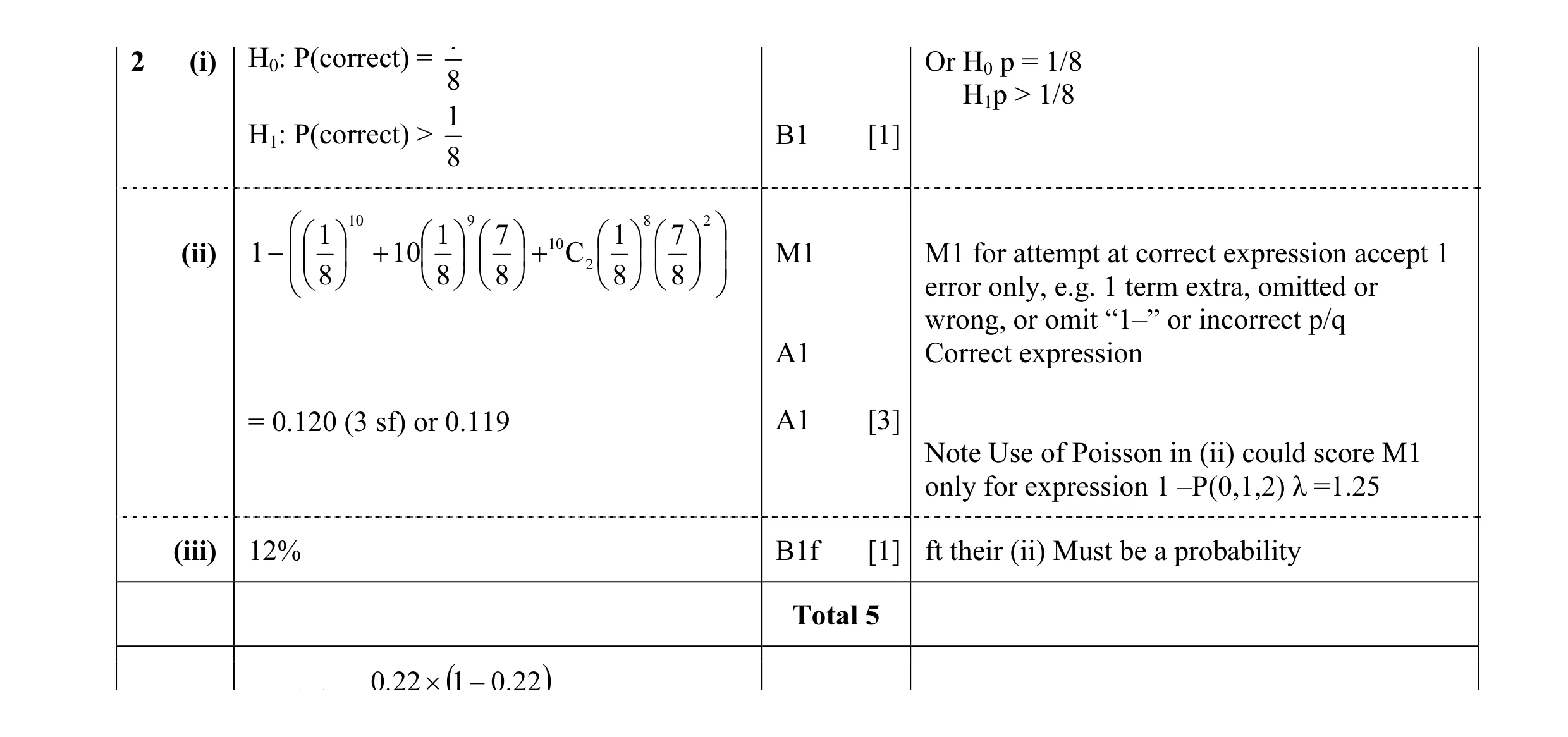 5
5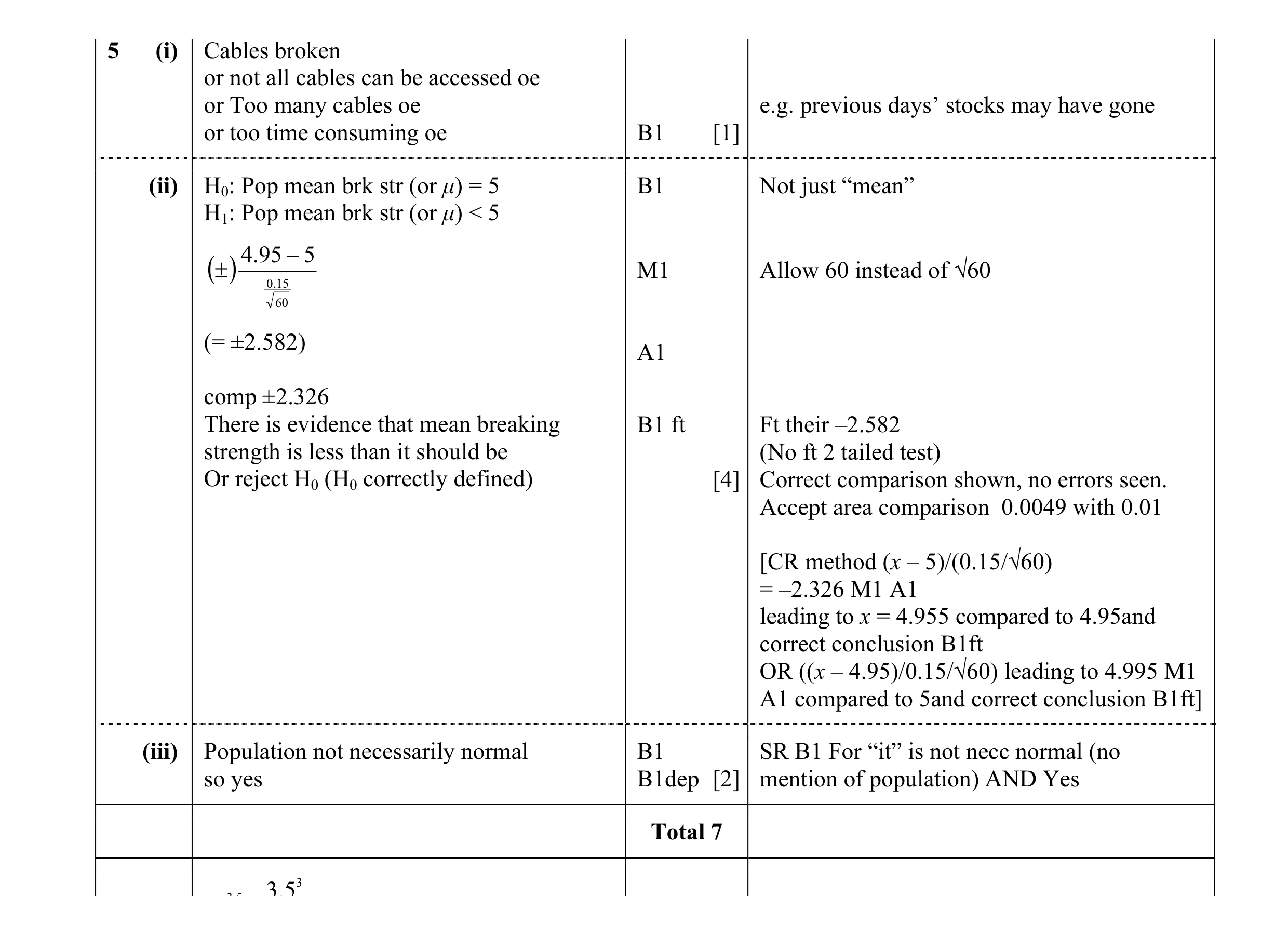 7
7 9
9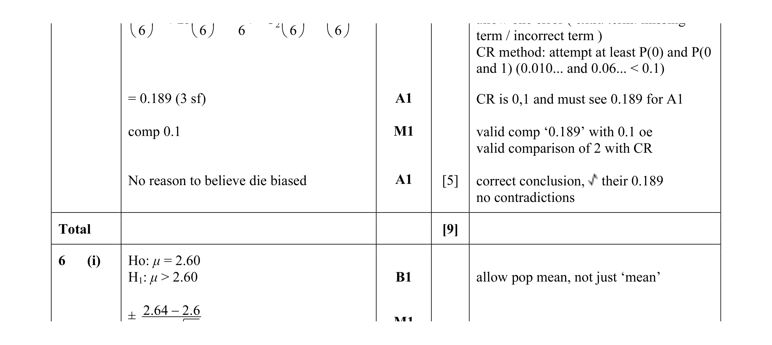 9
9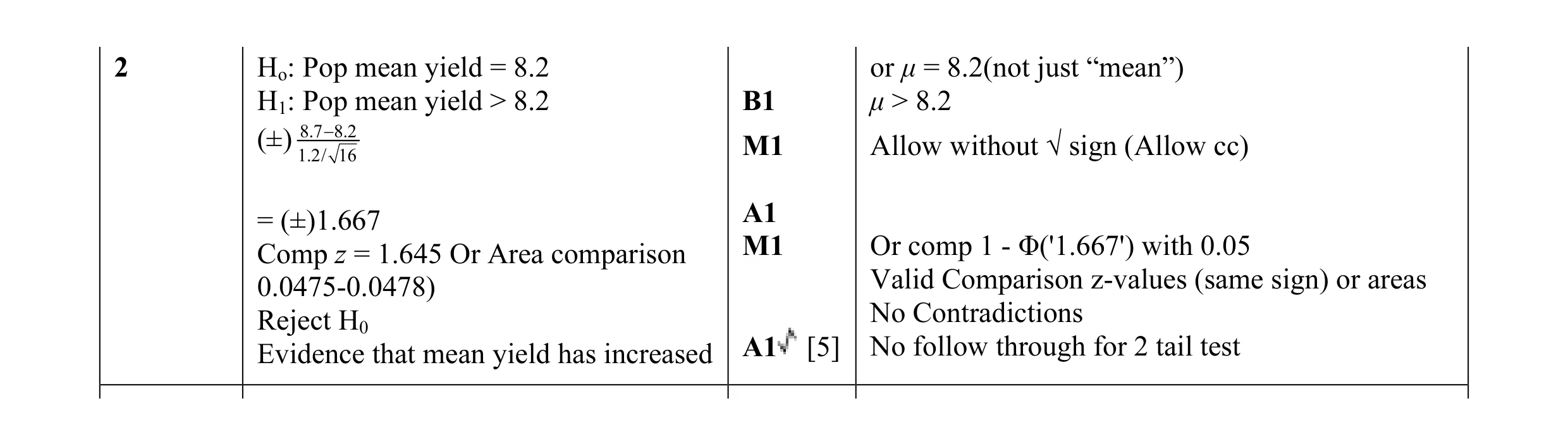 5
5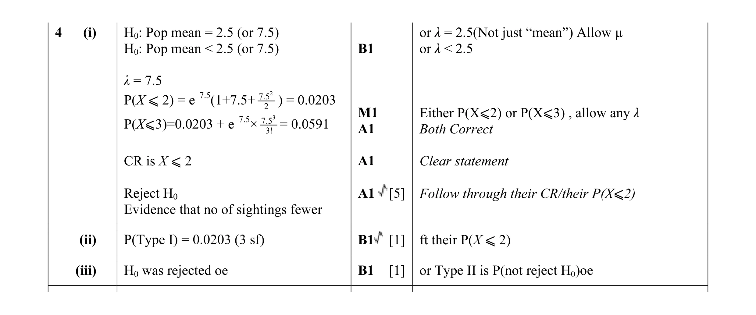 7
7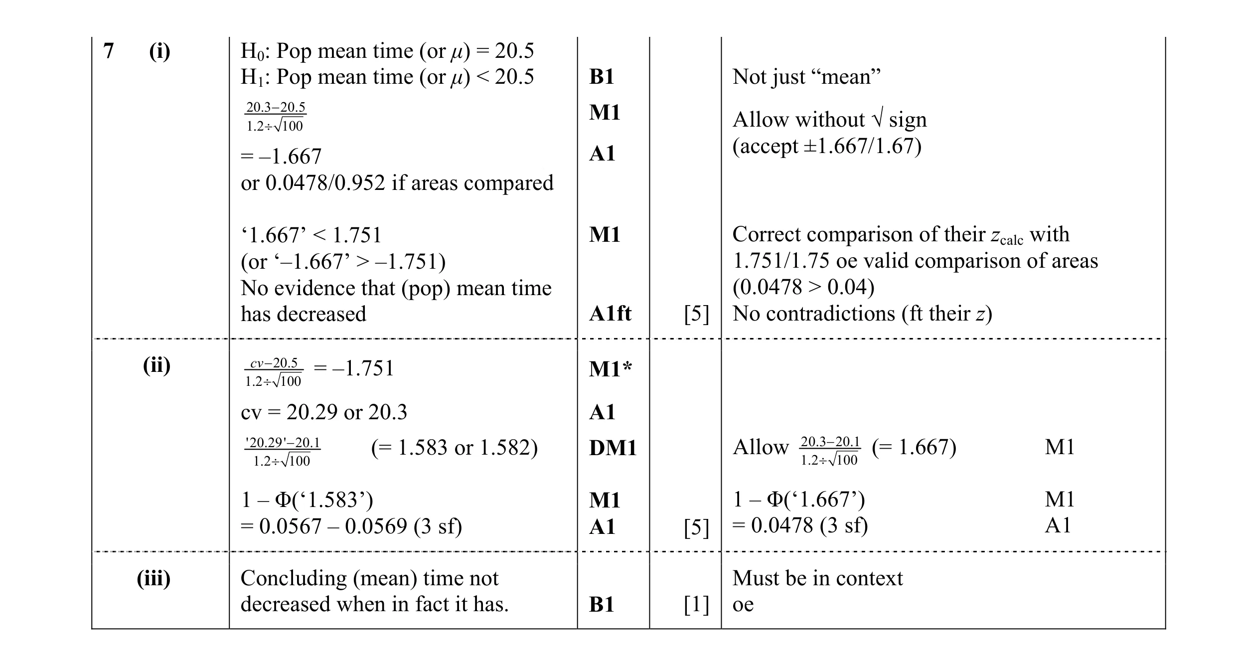 11
11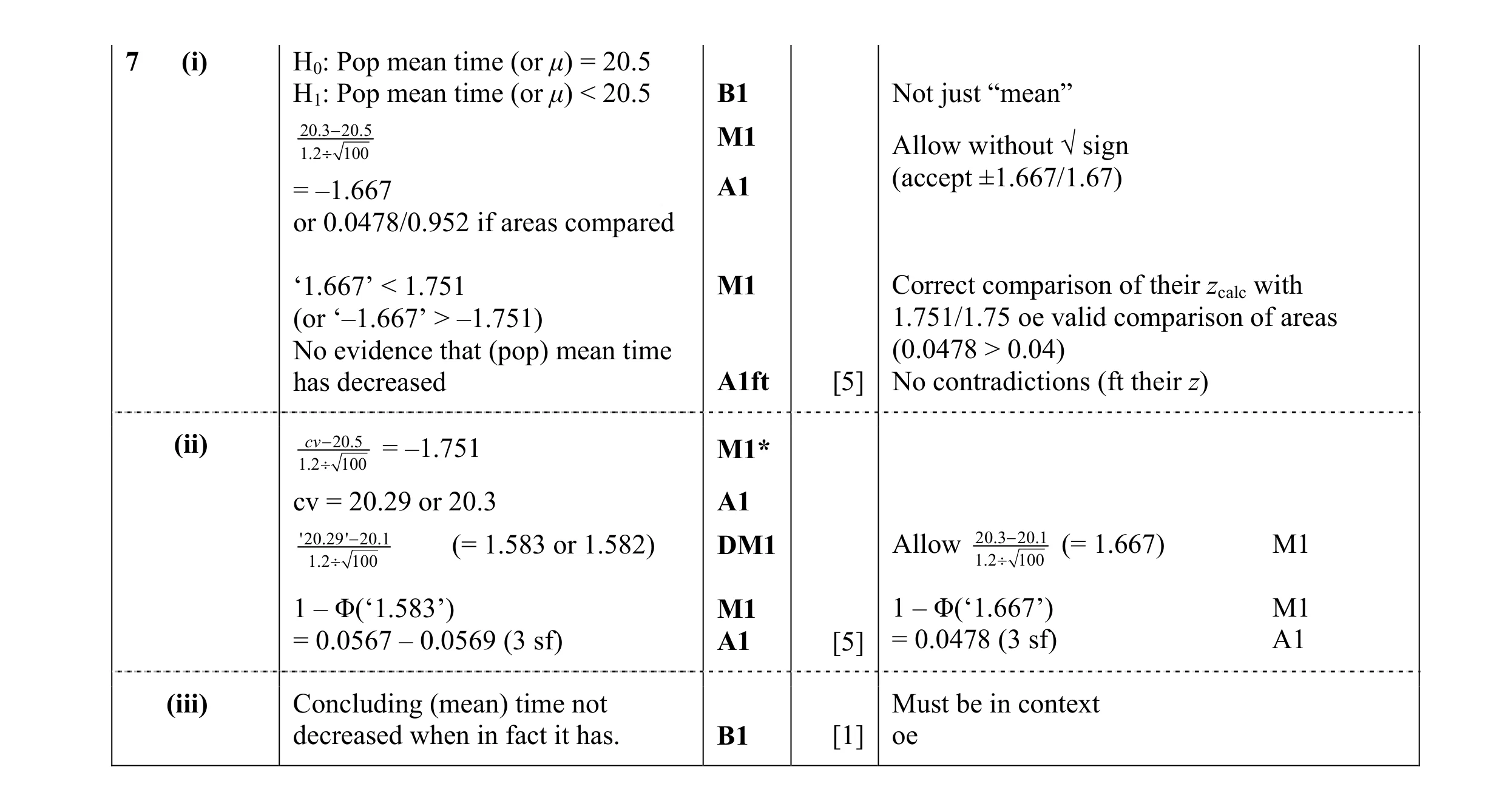 11
11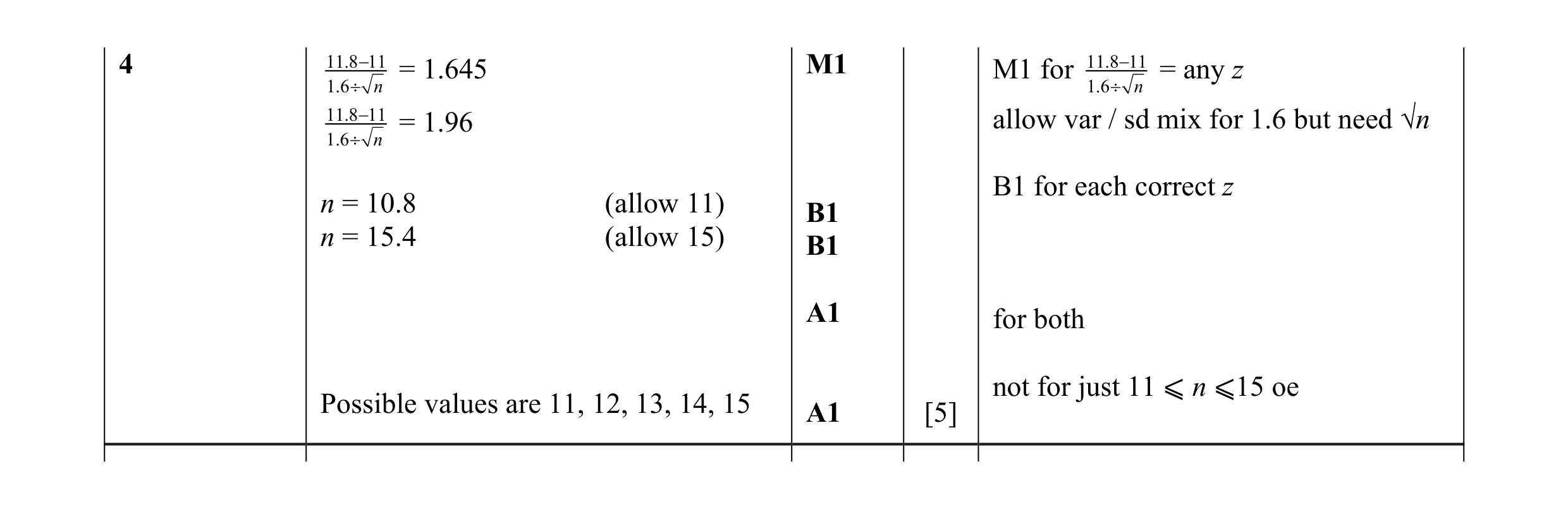 5
5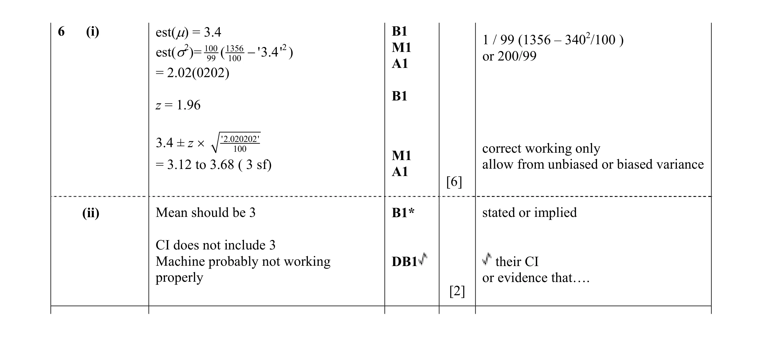 8
8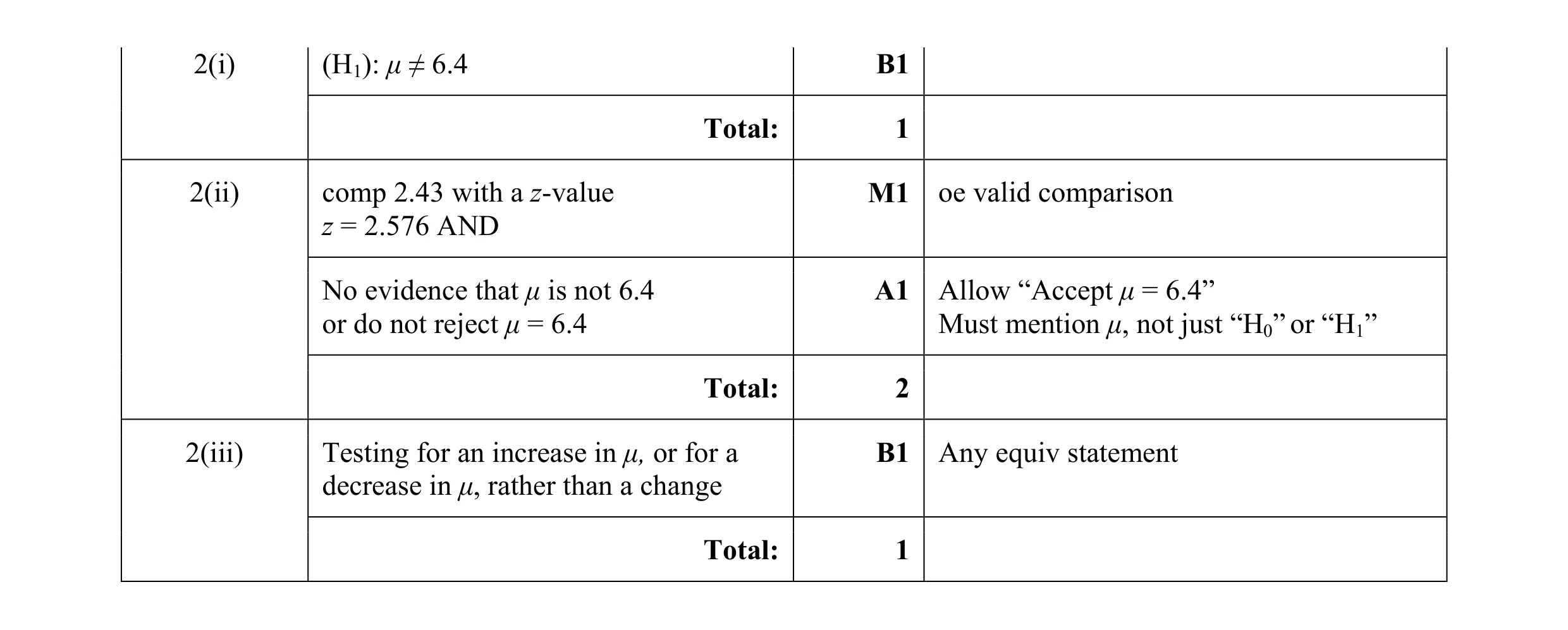 4
4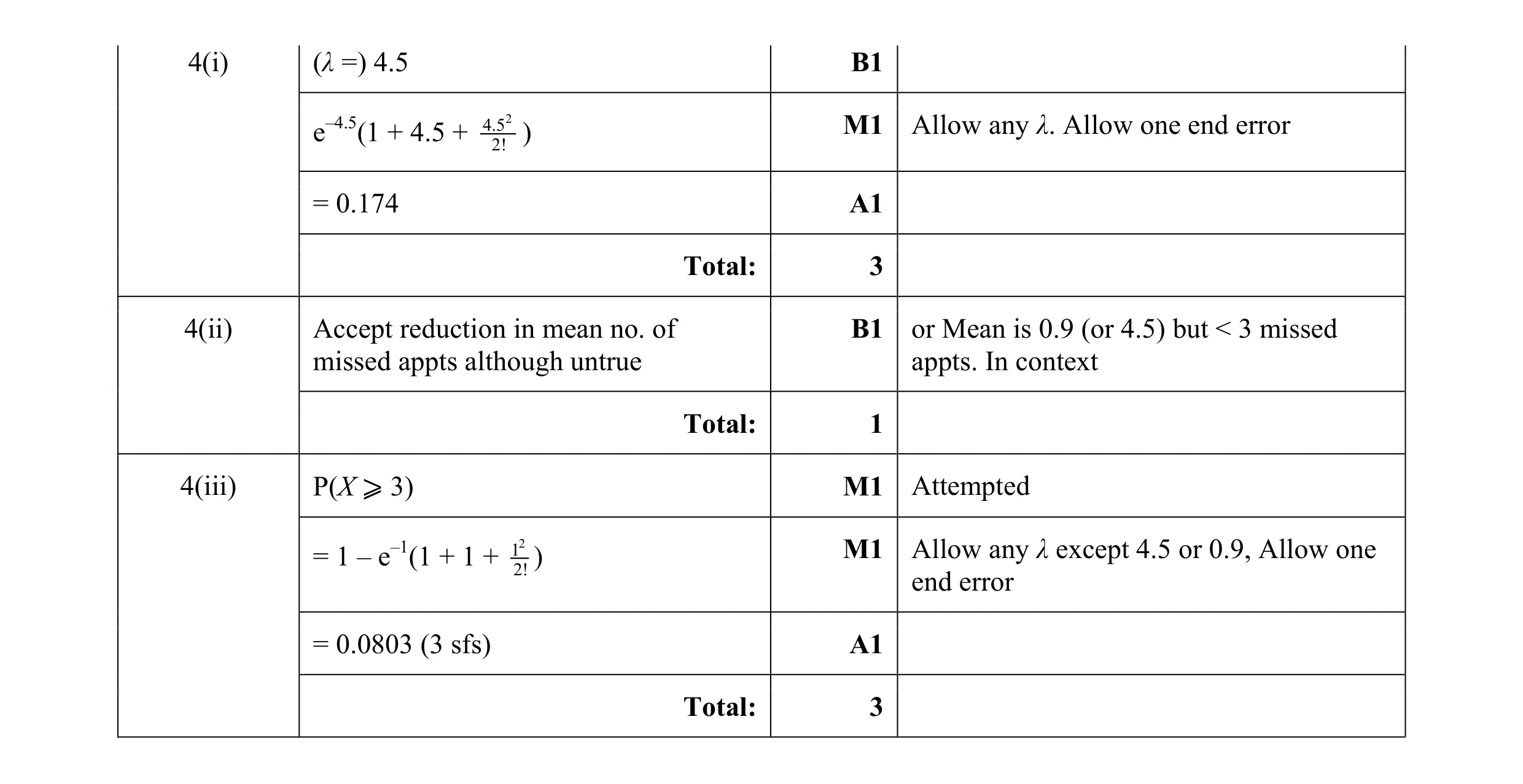 7
7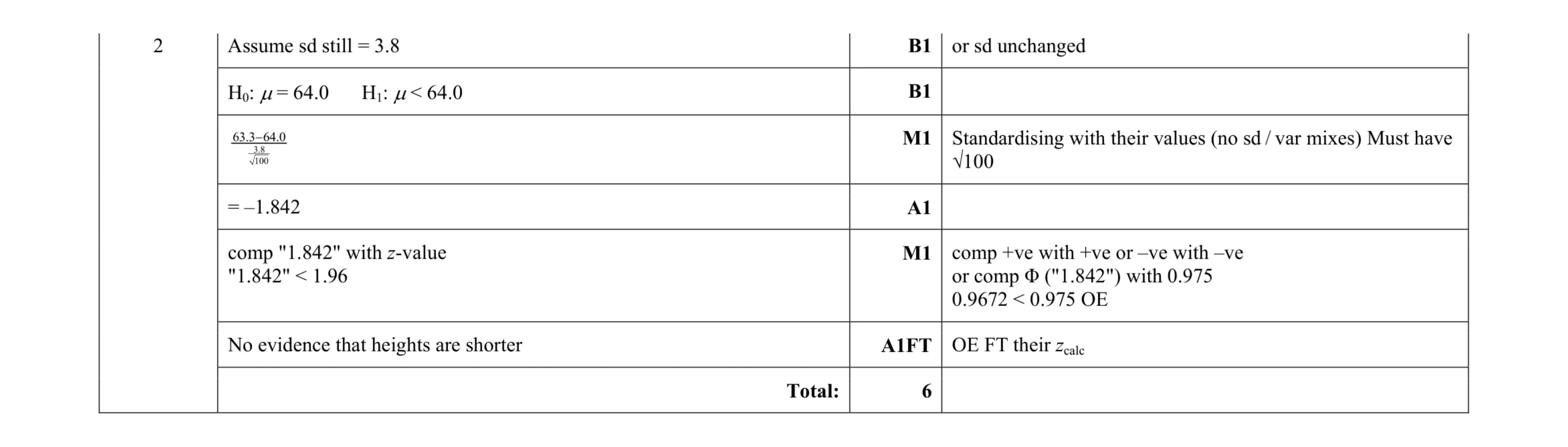 6
6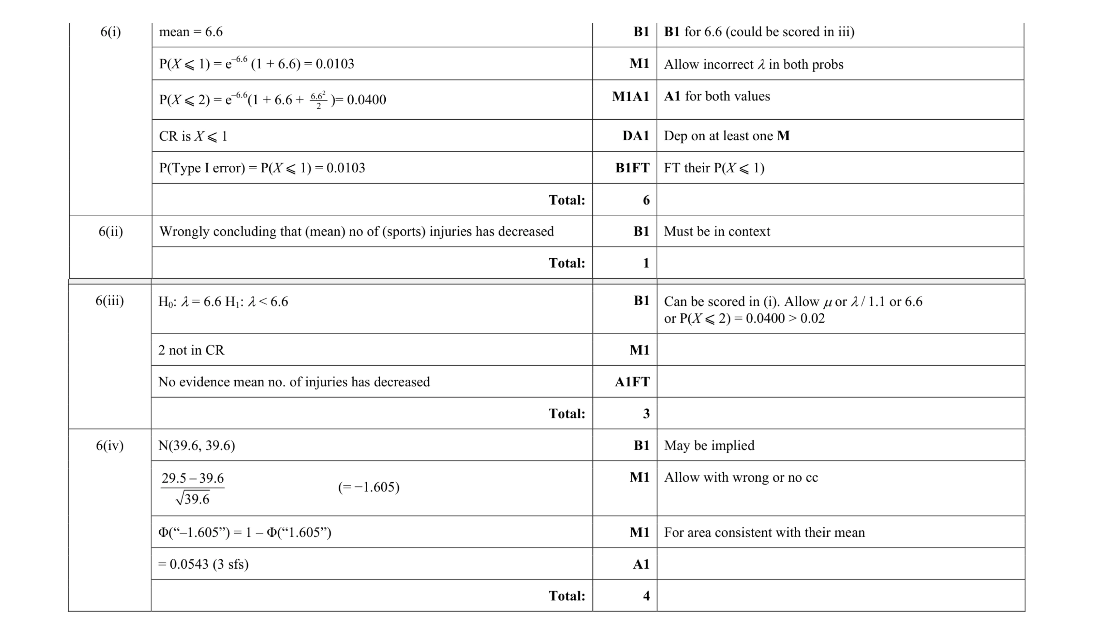 14
14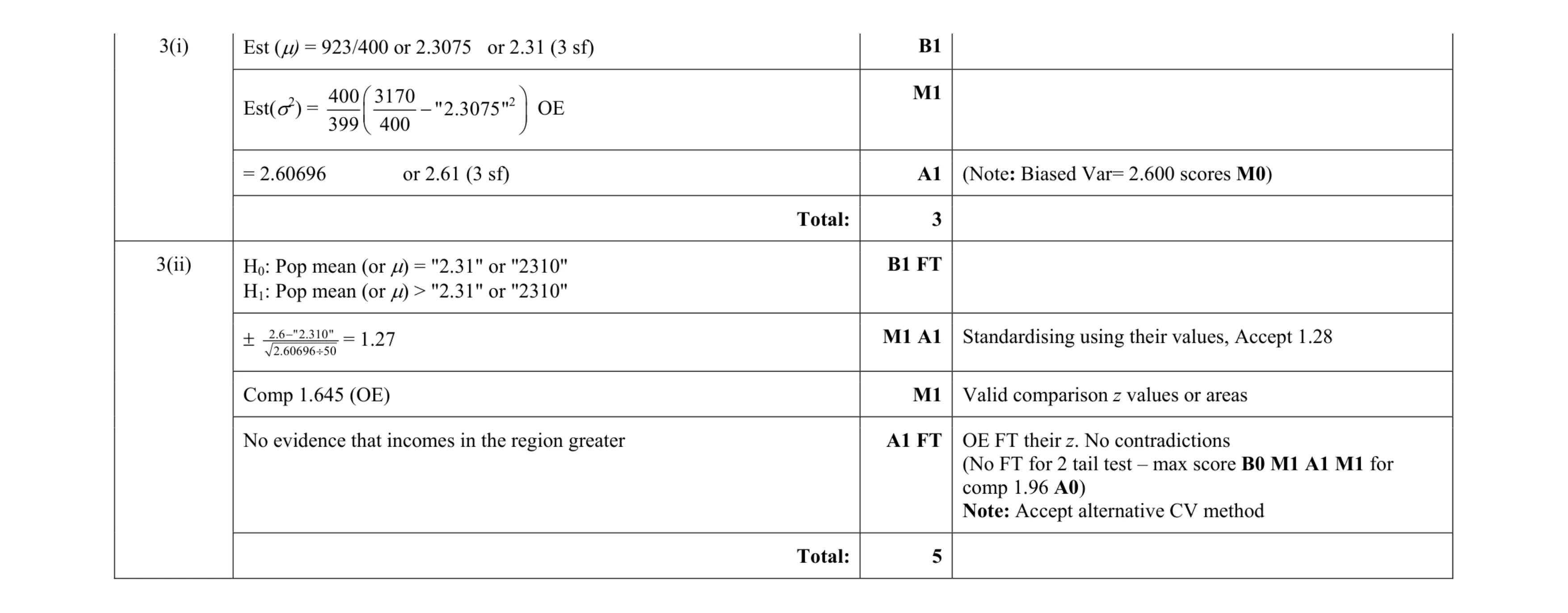 8
8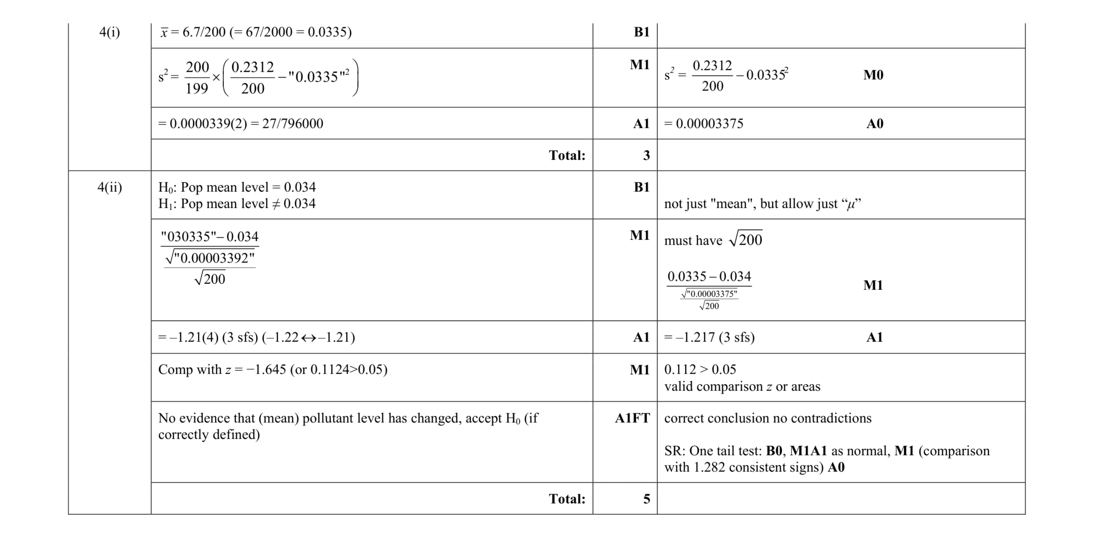 8
8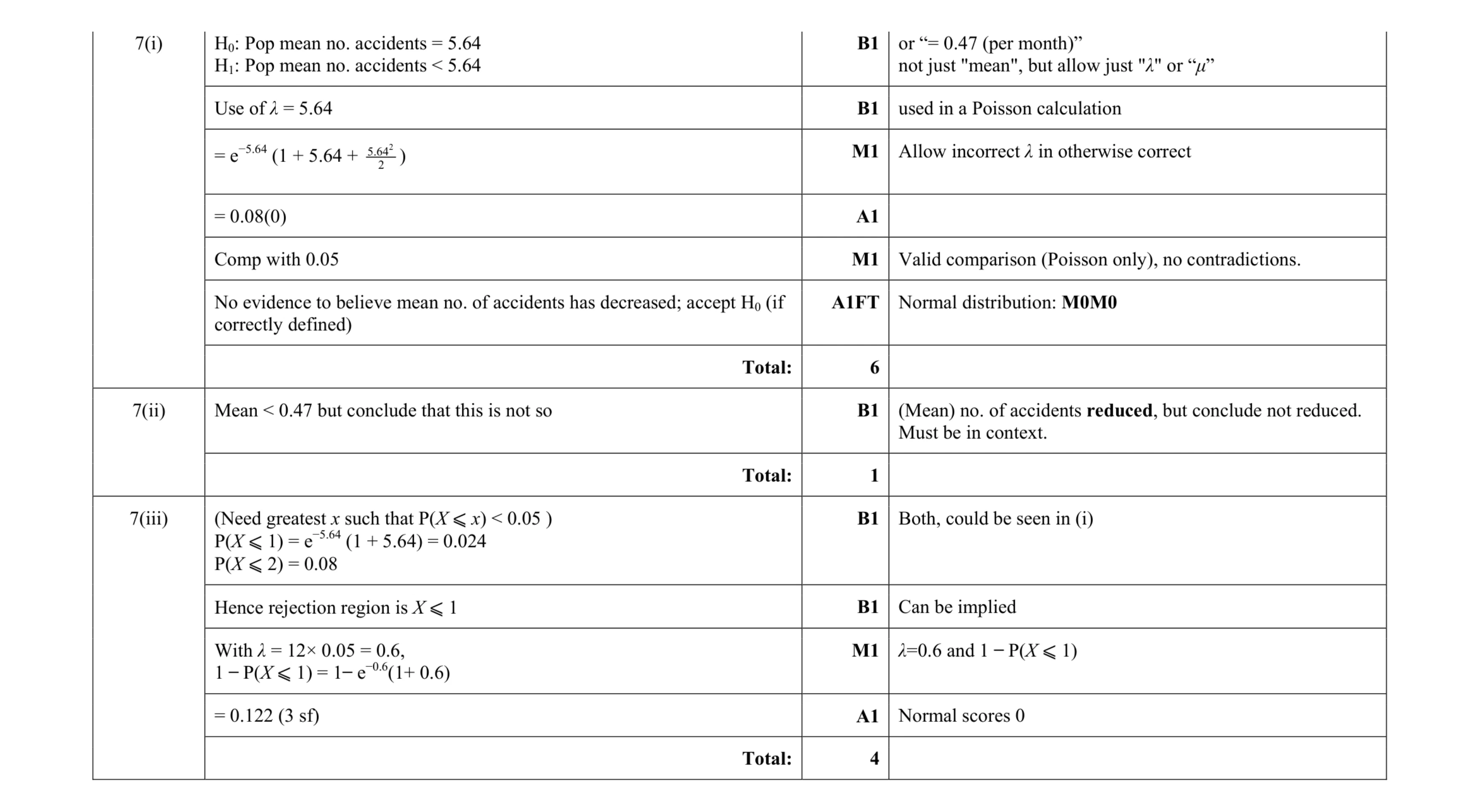 11
11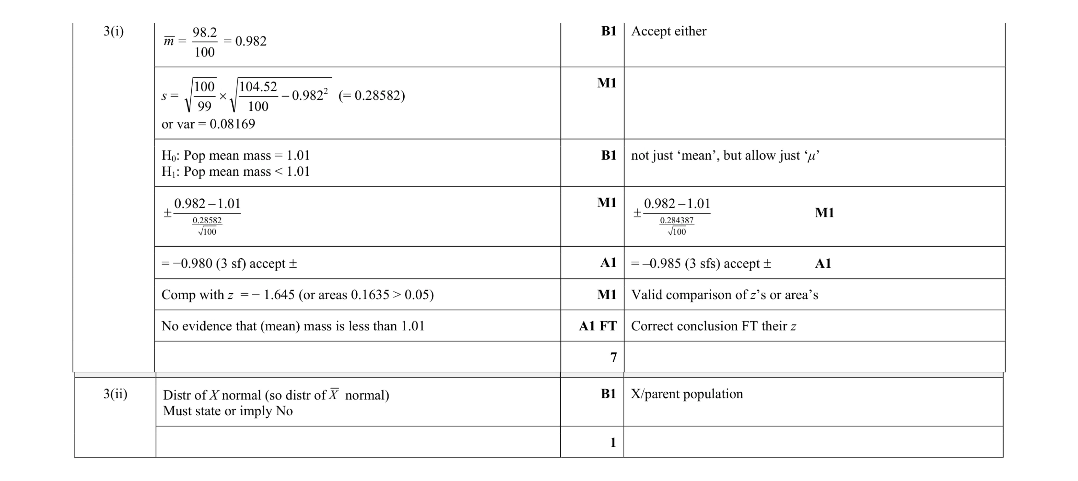 8
8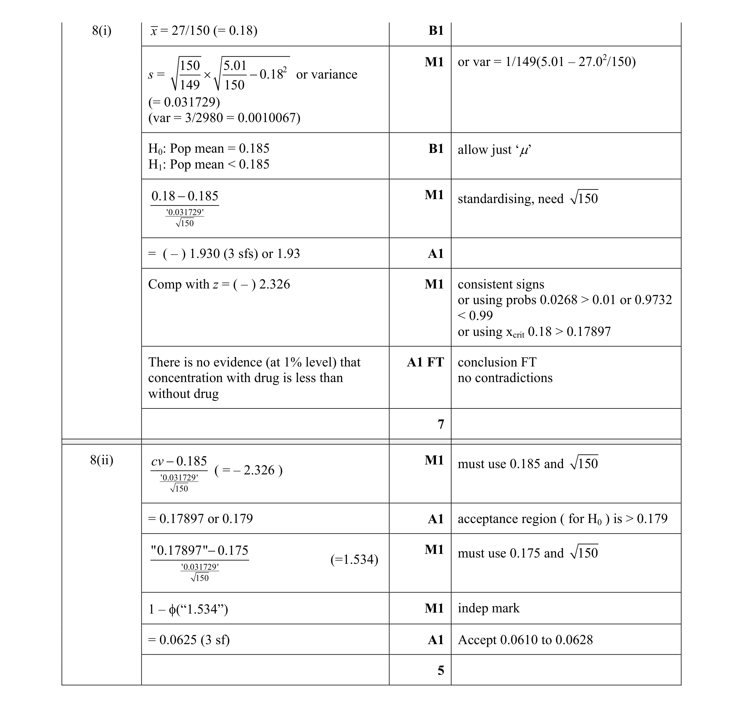 12
12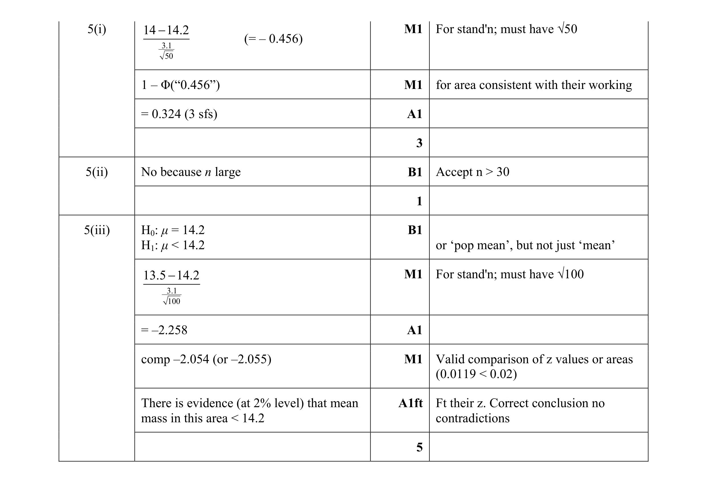 9
9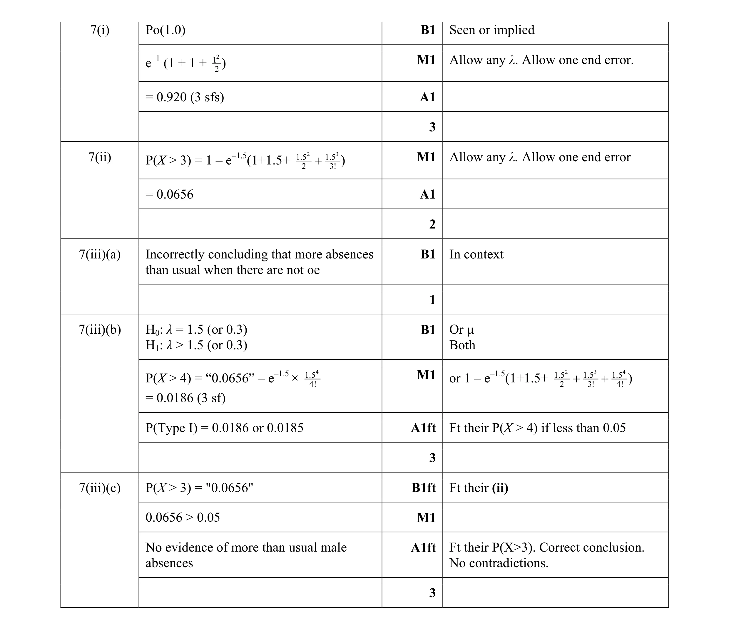 12
12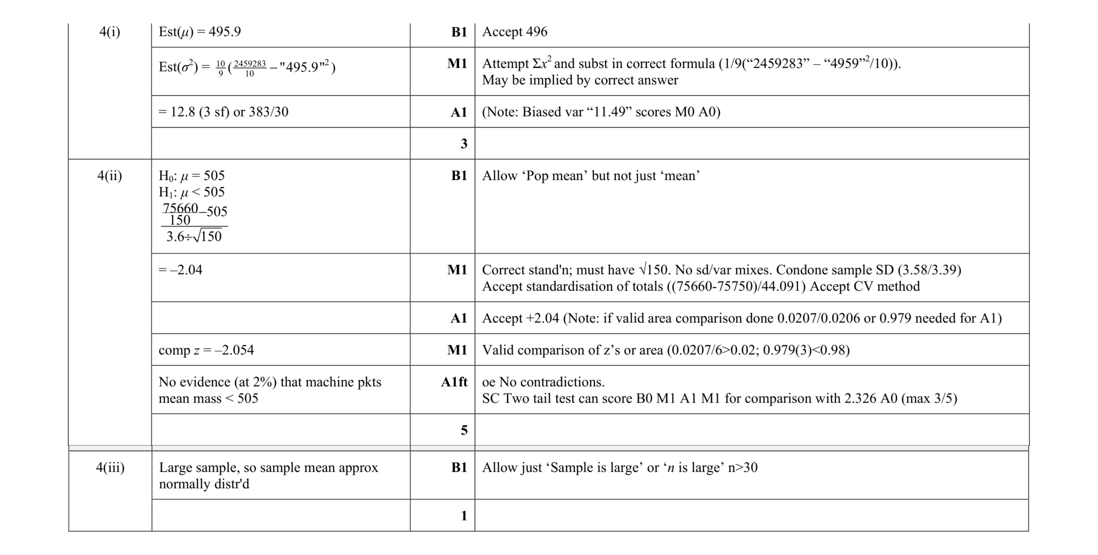 9
9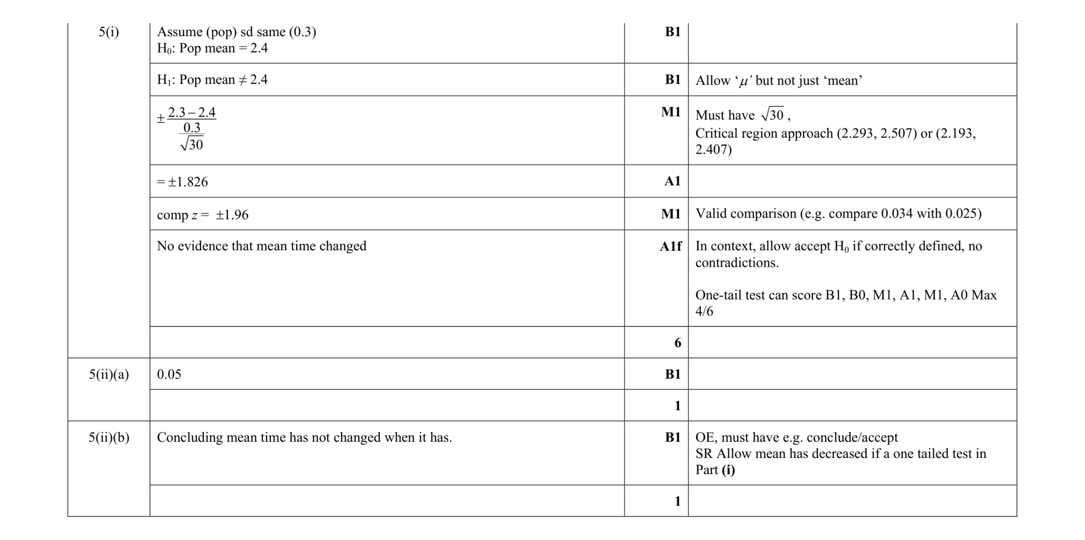 8
8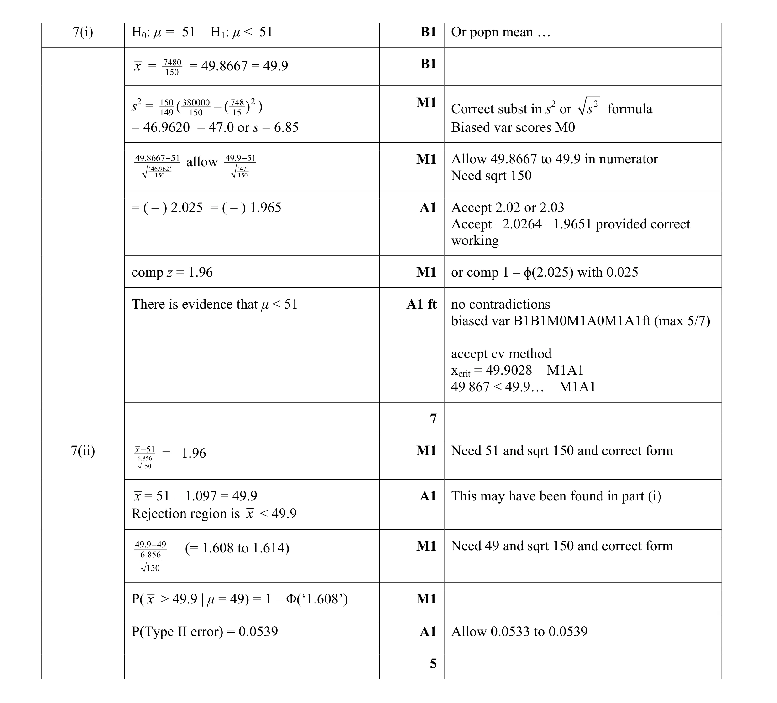 12
12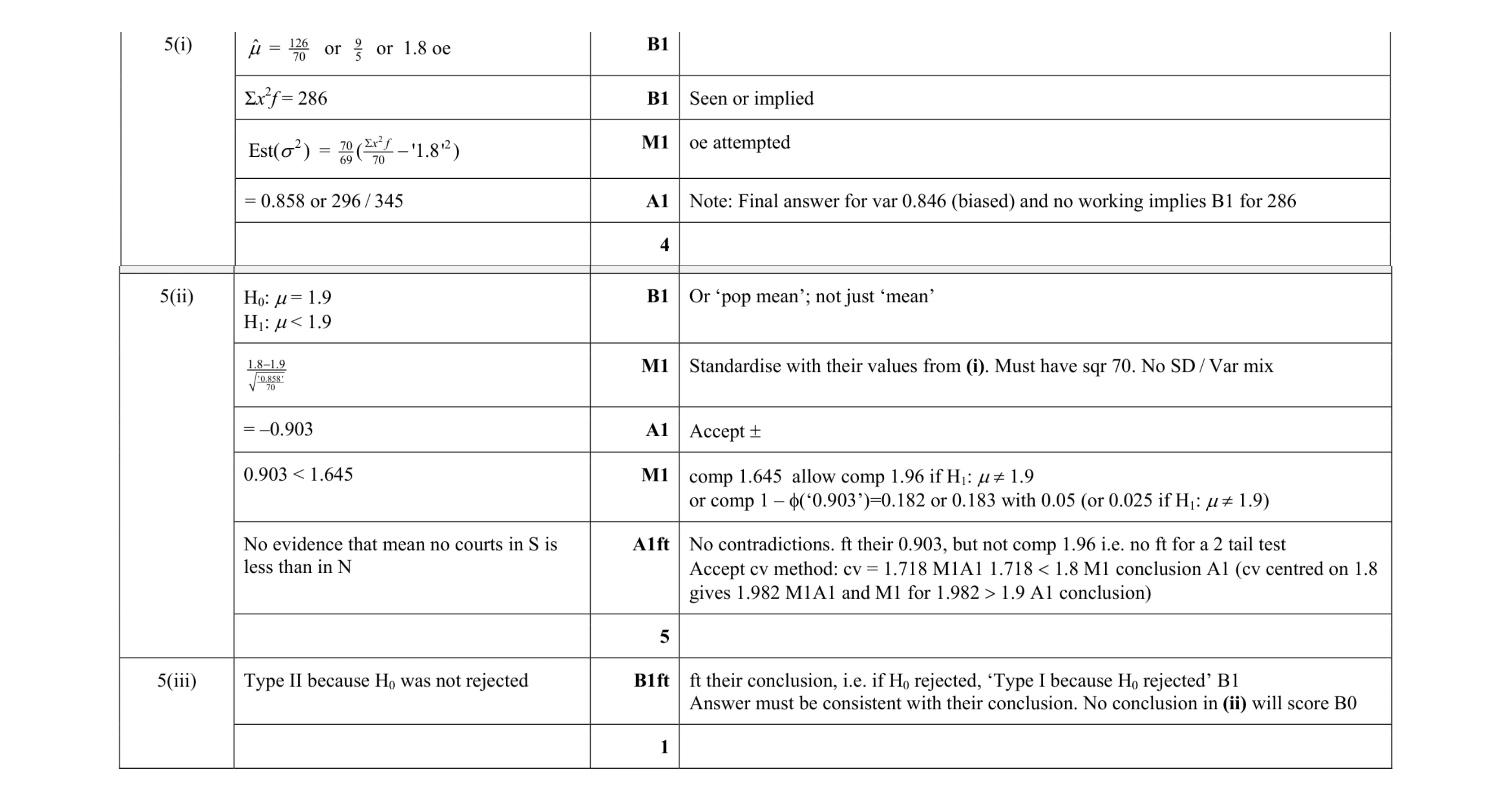 10
10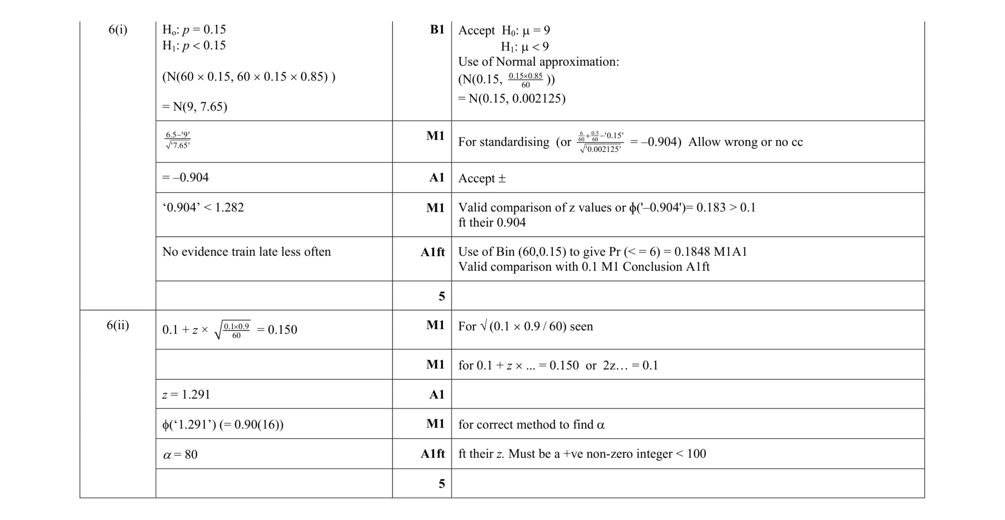 10
10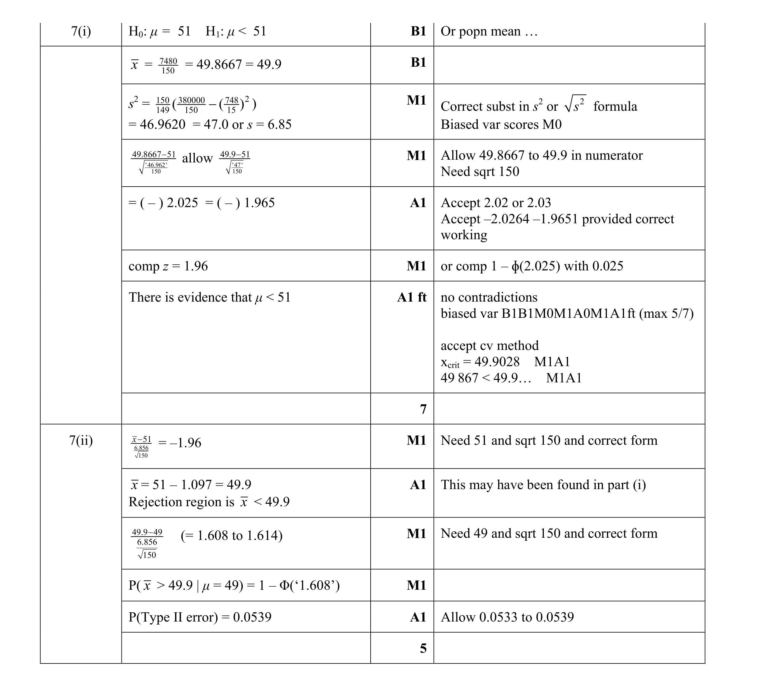 12
12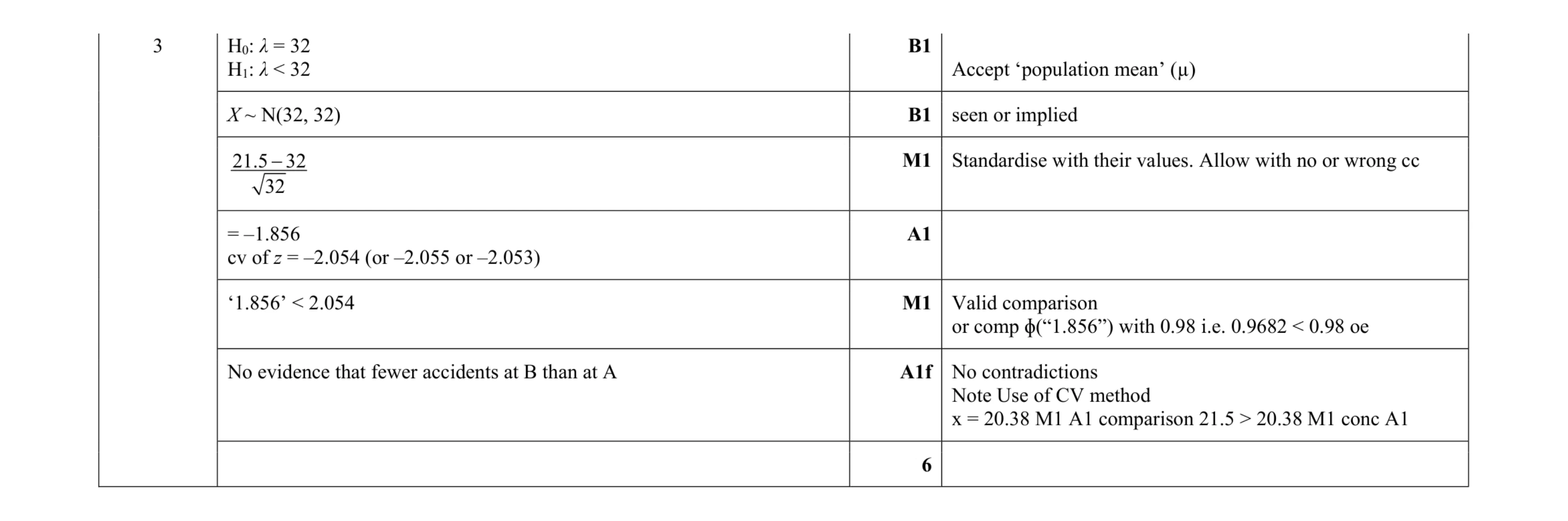 6
6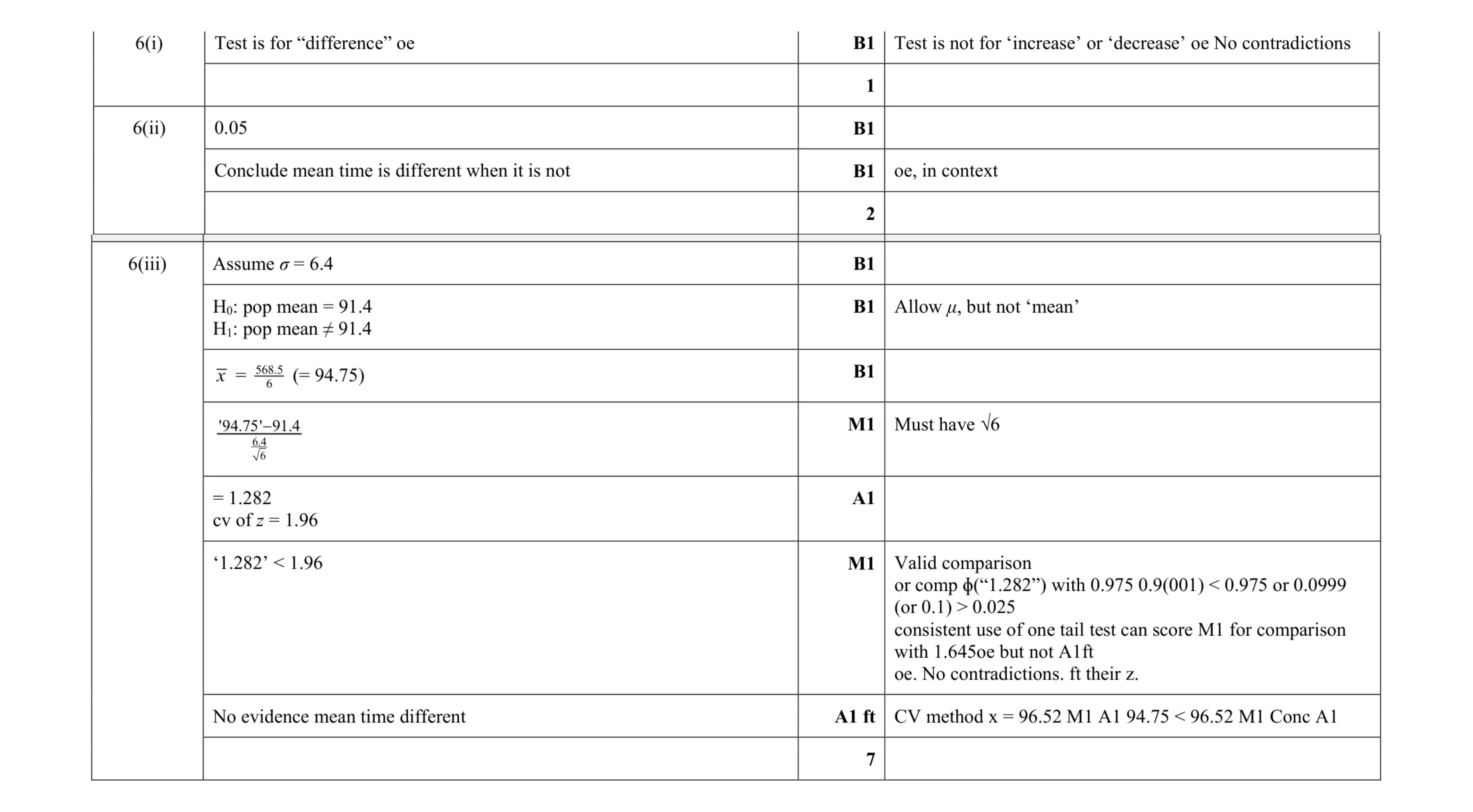 10
10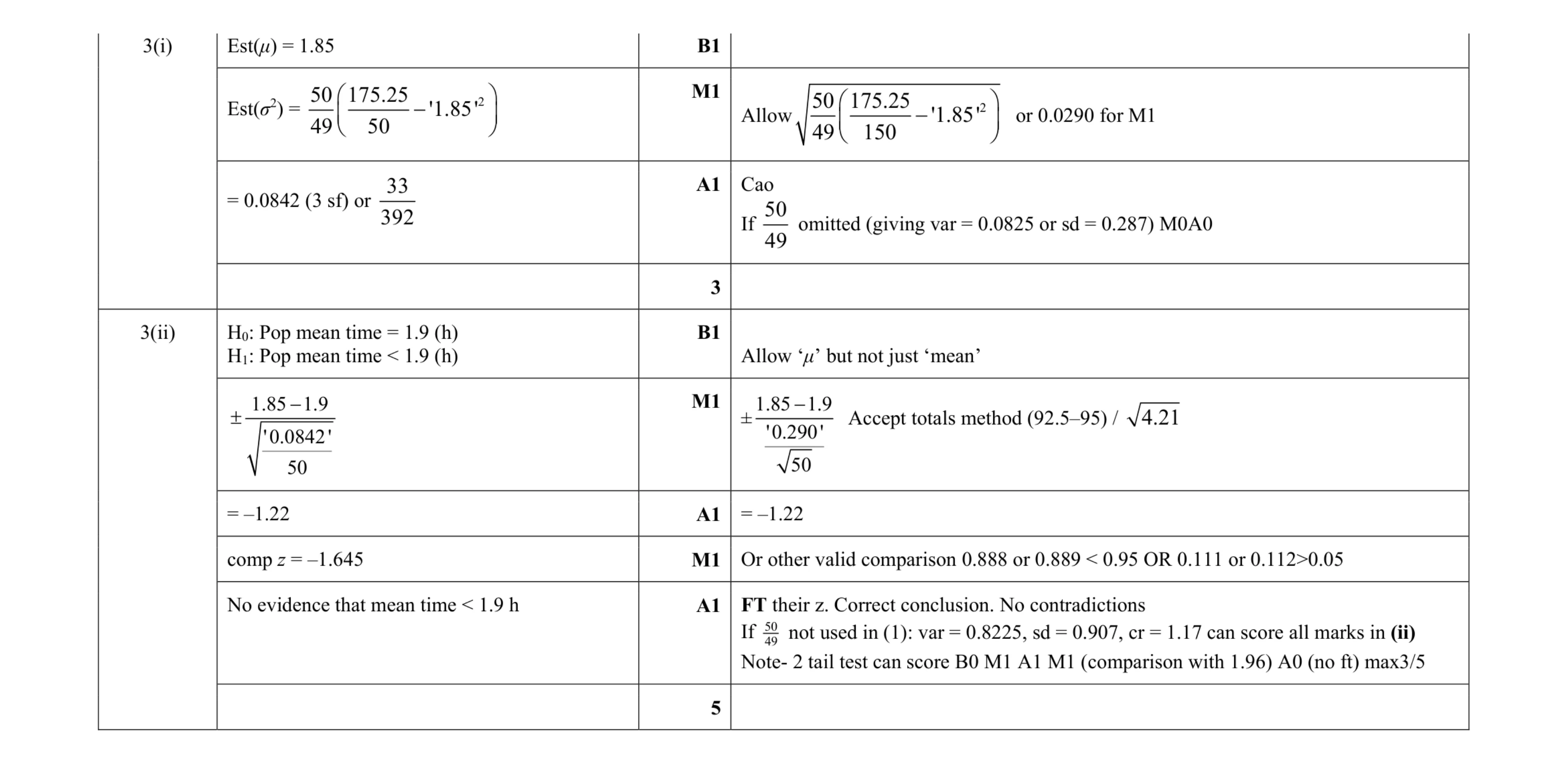 8
8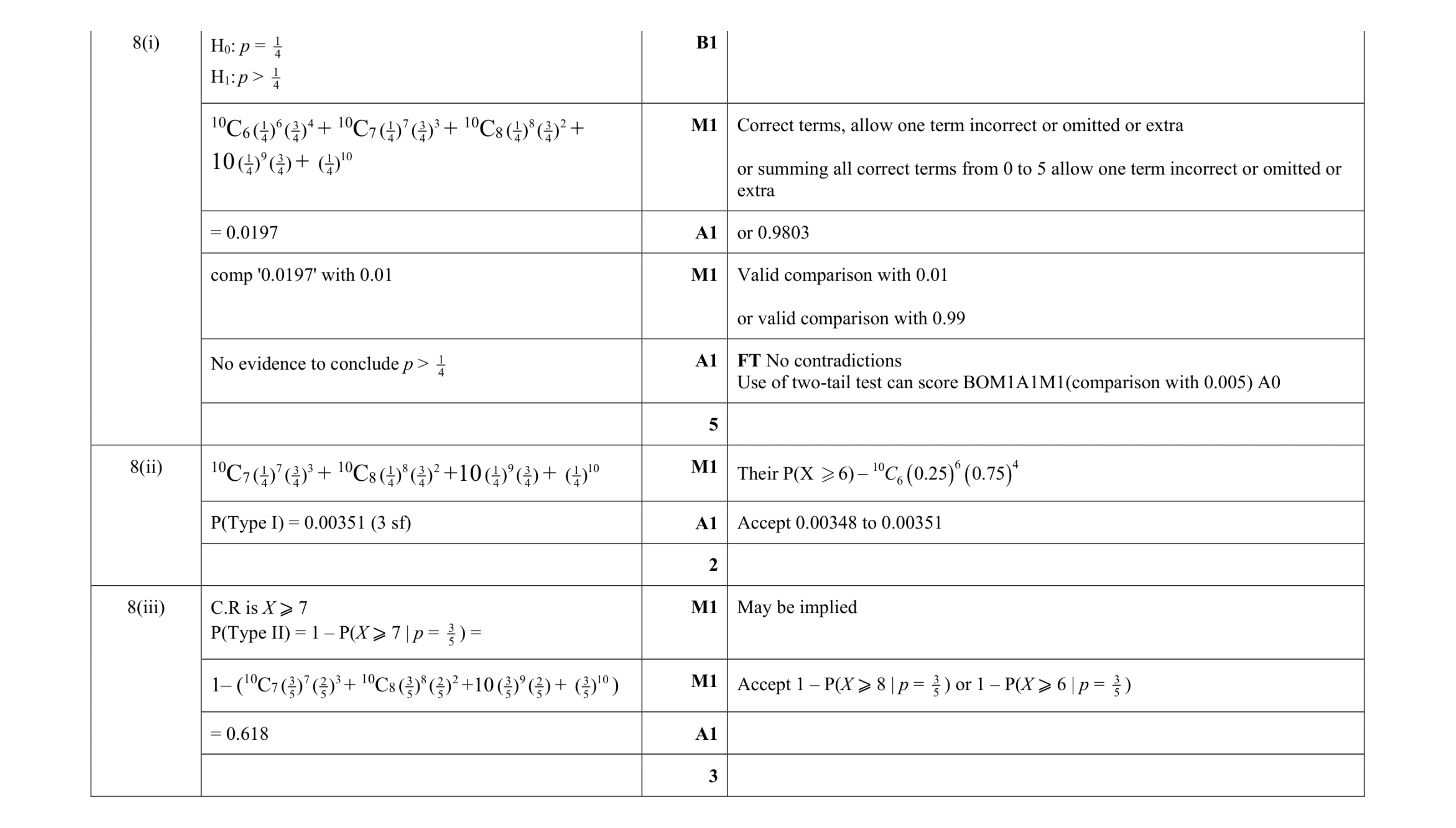 10
10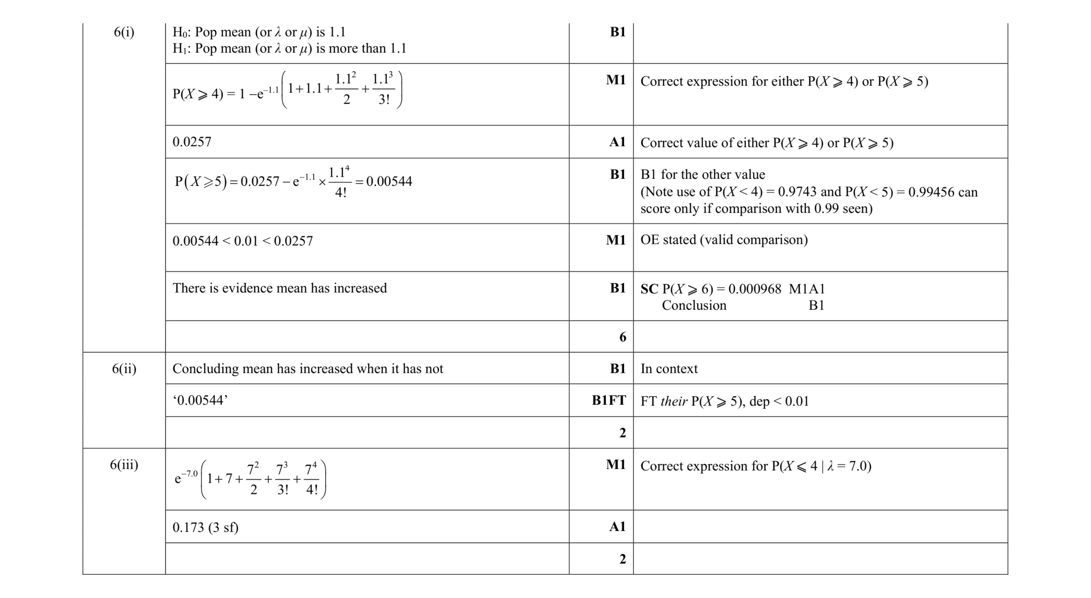 10
10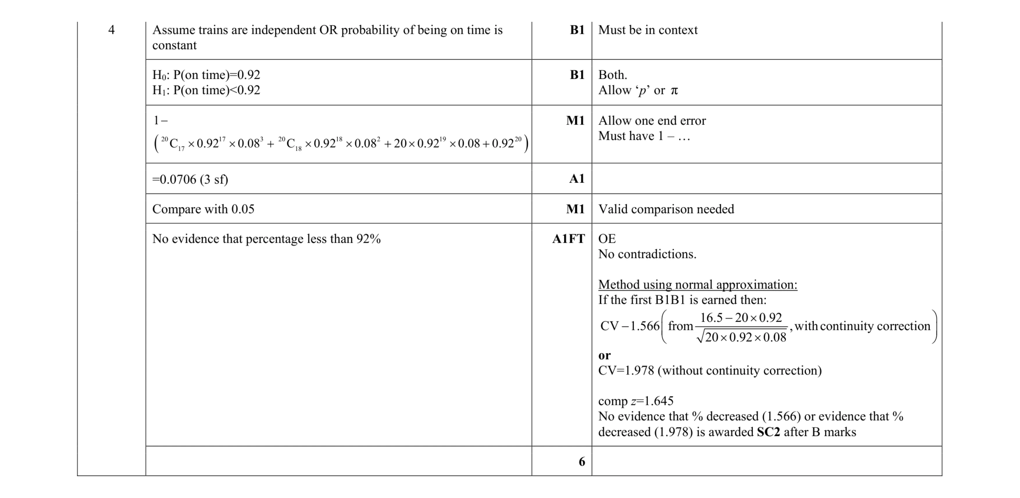 6
6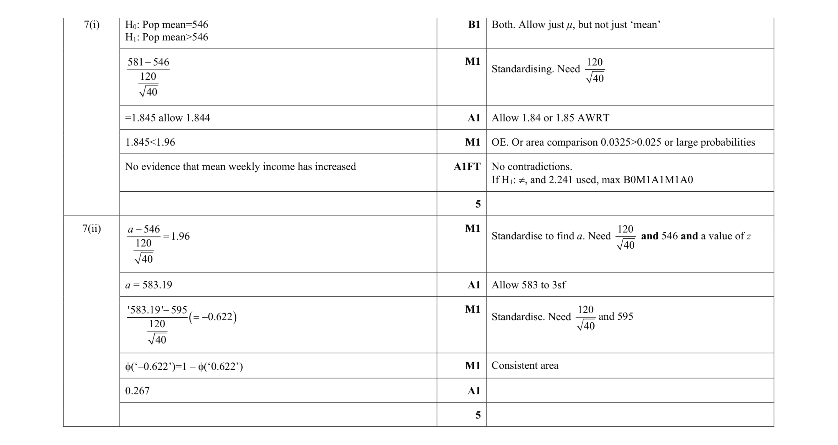 10
10