Questions as text
Q1 · In the past, the mean time taken by Freda for a particular daily journey was 39.2 minutes 9709/62 Feb/March 2020
3 In the past, the mean time taken by Freda for a particular daily journey was 39.2 minutes. Following the introduction of a one-way system, Freda wishes to test whether the mean time for the journey has decreased. She notes the times, t minutes, for 40 randomly chosen journeys and summarises the results as follows. n = 40 Σt = 1504 Σt2 = 57 760 (a) Calculate unbiased estimates of the population mean and variance of the new journey time. [3] … … … … … (b) Test, at the 5% significance level, whether the population mean time has decreased. [5] … … … … … … … … … … … … … … … …
8 marks
Mark scheme: 3(a) est (μ) = 37.6 or 1504 40 or 188 5 B1 est (σ2) = 2 40 57760 39 40 37.6 − = 31.0154 = 2016 65 M1 Correct substitution in any correct formula 2 1504 1 39 40 57760 − = 31.(0) (3 sf) A1 Accept 2016 65 or 1 65 31 3 3(b) H0: Pop mean (or μ) = 39.2 H1: Pop mean (or μ) < 39.2 B1 Both. Not just ‘mean’ 40 ' 0154 . 31 ' 2. 39 '6. 37 ' − M1 Allow use of biased variance (30.2), must have √40 = –1.817 A1 SC FT use of biased = –1.840 for A1 ‘1.817’ > 1.645 OE M1 Valid comparison ‘their 1.817’ with 1.645 or valid area comparison 0.0346 < 0.05 OE There is evidence that mean time has decreased A1FT FT their 1.817; in context, not definite, no contradictions SC For 2 tail test: H1: μ ≠ 39.2 and comp 1.96, max B0M1A1M1A0 (no FT for final mark) 5
This question in 9709/62 Feb/March 2020
Q2 · In the past the yield of a certain crop, in tonnes per hectare, had mean 0.56 and… 9709/61 May/June 2020
2 In the past the yield of a certain crop, in tonnes per hectare, had mean 0.56 and standard deviation 0.08. Following the introduction of a new fertilizer, the farmer intends to test at the 2.5% significance level whether the mean yield has increased. He finds that the mean yield over 10 years is 0.61 tonnes per hectare. (a) State two assumptions that are necessary for the test. [2] … … … … … … (b) Carry out the test. [5] … … … … … … … … … … … … … … …
7 marks
Mark scheme: 2(a) B1 Assume yields normally distributed B1 2 2(b) H0: Population mean yield (or μ) = 0.56 H1: Population mean yield (or μ) > 0.56 B1 0.61 0.56 0.08 10 − M1 1.976 A1 Comp 1.96 M1 There is evidence that mean yield has increased A1 5
This question in 9709/61 May/June 2020
Q3 · A market researcher is investigating the length of time that customers spend at an… 9709/63 May/June 2020
7 A market researcher is investigating the length of time that customers spend at an information desk. He plans to choose a sample of 50 customers on a particular day. (a) He considers choosing the first 50 customers who visit the information desk. Explain why this method is unsuitable. [1] … … … … … … … … The actual lengths of time, in minutes, that customers spend at the information desk may be assumed to have mean - and variance 4.8. The researcher knows that in the past the value of - was 6.0. He wishes to test, at the 2% significance level, whether this is still true. He chooses a random sample of 50 customers and notes how long they each spend at the information desk. (b) State the probability of making a Type I error and explain what is meant by a Type I error in this context. [2] … … … … … … … … … … (c) Given that the mean time spent at the information desk by the 50 customers is 6.8 minutes, carry out the test. [5] … … … … … … … … … … … … … … … … … (d) Give a reason why it was necessary to use the Central Limit theorem in your answer to part (c). [1] … … … … … …
9 marks
Mark scheme: 7(a) Later customers might spend times different from first ones B1 1 7(b) 0.02 B1 Concluding that μ ≠ 6.0, when actually μ = 6.0 B1 2 Question Answer Marks 7(c) H0: μ = 6.0 H1: μ ≠ 6.0 B1 6.8 6.0 4.8 50 − M1 2.582 A1 comp 2.326 M1 Evidence that μ ≠ 6.0 A1 5 7(d) Population distribution unknown B1 1
This question in 9709/63 May/June 2020
Q4 · The number of absences per week by workers at a factory has the distribution Po 2.1 9709/61 Oct/Nov 2020
5 The number of absences per week by workers at a factory has the distribution Po 2.1 . (a) Find the standard deviation of the number of absences per week. [1] … … … (b) Find the probability that the number of absences in a 2-week period is at least 2. [3] … … … … … … … … … (c) Find the probability that the number of absences in a 3-week period is more than 4 and less than 8. [2] … … … … … … … … … Following a change in working conditions, the management wished to test whether the mean number of absences has decreased. They found that, in a randomly chosen 3-week period, there were exactly 2 absences. (d) Carry out the test at the 10% significance level. [5] … … … … … … … … … … … … … … … (e) State, with a reason, which of the errors, Type I or Type II, might have been made in carrying out the test in part (d). [2] … … … … … …
13 marks
Mark scheme: 5(a) √2.1 or 1.45 (3 sf) B1 1 5(b) λ = 4.2 B1 1 – e–4.2(1 + 4.2) M1 1 – P(X ⩽ 1) any λ, allow one end error. = 0.922 (3 sf) A1 3 5(c) λ = 6.3 5 6 7 6.3 6.3 6.3 6.3 e 5! 6! 7! − + + M1 P(X = 5, 6, 7) any λ, allow one end error. = 0.455 (3 sf) A1 2 5(d) H0: λ = 6.3 H1: λ < 6.3 B1 Accept µ, accept 2.1 (per week) P(X ⩽ 2) = 2 6.3 6.3 e 1 6.3 2! − + + M1 = 0.0498 or 0.0499 A1 Accept 0.0499 ‘0.0498’ < 0.1 M1 For valid comparison. For CV method the comparison can be ‘2 lies in CR of X ⩽ 2’ There is evidence that mean number of absences has decreased. A1 FT In context, not definite, e.g. not ‘Mean number of absences has decreased.’ No contradictions. 5 Question Answer Marks Guidance 5(e) H0 rejected *B1 FT OE Hence Type I error possible DB1 FT 2
This question in 9709/61 Oct/Nov 2020
Q5 · The time, in minutes, for Anjan’s journey to work on Mondays has mean 38.4 and standard… 9709/61 Oct/Nov 2020
6 The time, in minutes, for Anjan’s journey to work on Mondays has mean 38.4 and standard deviation 6.9. (a) Find the probability that Anjan’s mean journey time for a random sample of 30 Mondays is between 38 and 40 minutes. [5] … … … … … … … … … … … … … … … … … … … … … … … Anjan wishes to test whether his mean journey time is different on Tuesdays. He chooses a random sample of 30 Tuesdays and finds that his mean journey time for these 30 Tuesdays is 40.2 minutes. Assume that the standard deviation for his journey time on Tuesdays is 6.9 minutes. (b) (i) State, with a reason, whether Anjan should use a one-tail or a two-tail test. [1] … … … … (ii) Carry out the test at the 10% significance level. [5] … … … … … … … … … … … … (iii) Explain whether it was necessary to use the Central Limit theorem in part (b)(ii). [1] … … … … …
12 marks
Mark scheme: 6(a) 40 38.4 6.9 30 − = 1.270 38 38.4 6.9 30 − = –0.3175 M1 M1 for either correct expression must have √30 (condone continuity correction) A1 A1 for ±1.270 or for 1.27 or AWRT A1 A1 for ± (–0.3175) must be opposite sign or for 0.317 or 0.318 or AWRT Φ(‘1.270’) – (1 – ɸ('0.3175') M1 For correct method consistent with their values = 0.523 (3 sf) or 0.522 A1 5 6(b)(i) 2-tail because looking for ‘change’, not decrease or increase B1 OE 1 Question Answer Marks Guidance 6(b)(ii) H0: Population mean journey time (or μ) = 38.4 H1: Population mean journey time (or μ) ≠ 38.4 B1 Not just ‘mean journey time’ 40.2 38.4 6.9 30 − M1 For standardising (must have √30 ) = 1.429 A1 ‘1.429’ < 1.645 M1 For valid comparison (area comparison 0.0765 > 0.05 ) There is no evidence that mean journey time has changed. A1 FT In context. Not definite (e.g. not ‘mean journey time has not changed’). No contradictions. FT their ‘1.429’ (Note use of 1-tail test scores B0 M1A1M1(comparison with 1.282) A0 max) Alternative method for question 6(b)(ii) – critical values method H0: Population mean journey time (or μ) = 38.4 H1: Population mean journey time (or μ) ≠ 38.4 B1 Not just ‘mean journey time’ 6.9 38 1.645 30 + M1 = 40.47 A1 40.2 < 40.47 M1 For valid comparison There is no evidence that mean journey time has changed. A1 FT In context. Not definite (e.g. not ‘mean journey time has not changed’). No contradictions. 5 Question Answer Marks Guidance 6(b)(iii) Yes, because population distribution unknown. B1 Allow: Yes, because population distribution not normal. 1
This question in 9709/61 Oct/Nov 2020
Q6 · The areas, X cm2, of petals of a certain kind of flower have mean - cm2 9709/62 Oct/Nov 2020
4 The areas, X cm2, of petals of a certain kind of flower have mean - cm2. In the past it has been found that - = 8.9. Following a change in the climate, a botanist claims that the mean is no longer 8.9. The areas of a random sample of 200 petals from this kind of flower are measured, and the results are summarized by Σx = 1850, Σx2 = 17 850. Test the botanist’s claim at the 2.5% significance level. [8] … … … … … … … … … … … … … … … … … … … … … … … … … … … … … … … … … … … … … … … … … … … … … … …
8 marks
Mark scheme: 4 est(μ) = 1850 200 or 9.25 B1 est(σ2) = 2 200 17850 1850 199 200 200 − or 2 1 1850 199 200 17850 − M1 = 3.71 or 3.7060 or 1475 398 A1 H0: μ = 8.9 H1: μ ≠ 8.9 B1 Accept Population mean (not just mean) 1850 8.9 200 "3.706" 200 − M1 Use of biased variance (3.6875) still scores M1 = 2.57(3sf) (or using areas 0.00507 – 0.0051) A1 Accept 2.58 (3sf) or using areas 0.0049–0.005 where biased variance used. 2.24 < 2.57 or 0.00507 < 0.0125 M1 For valid comparison with 2.240 or 2.241 or valid comparison with 0.0125 Accept 2.24 < 2.58 or 0.00496 < 0.0125 where biased variance used (Reject H0) There is evidence that μ is not 8.9 A1 FT Not definite, e.g. NOT ‘μ ≠ 8.9’ Must be in context. No contradictions. (Accept cv method) (Note: Use of 1 tail test scores Max B1M1A1B0M1A1M1A0, max 6 out of 8) 8
This question in 9709/62 Oct/Nov 2020
Q7 · A biscuit manufacturer claims that, on average, 1 in 3 packets of biscuits contain a… 9709/62 Oct/Nov 2020
6 A biscuit manufacturer claims that, on average, 1 in 3 packets of biscuits contain a prize offer. Gerry suspects that the proportion of packets containing the prize offer is less than 1 in 3. In order to test the manufacturer’s claim, he buys 20 randomly selected packets. He finds that exactly 2 of these packets contain the prize offer. (a) Carry out the test at the 10% significance level. [5] … … … … … … … … … … … … … … … … … … … … … … … (b) Maria also suspects that the proportion of packets containing the prize offer is less than 1 in 3. She also carries out a significance test at the 10% level using 20 randomly selected packets. She will reject the manufacturer’s claim if she finds that there are 3 or fewer packets containing the prize offer. Find the probability of a Type II error in Maria’s test if the proportion of packets containing the prize offer is actually 1 in 7. [3] … … … … … … … … … … … … … … … (c) Explain what is meant by a Type II error in this context. [1] … … … … … …
9 marks
Mark scheme: 6(a) H0: P(contains offer) = 1 3 H1: P(contains offer) < 1 3 B1 Allow p for P(contains offer) but not just proportion P(0,1 or 2 offers in 20 | H0) = 20 2 3 + 20 19 2 3 1 3 + 20C2 18 2 3 2 1 3 M1 = 0.0176 (3sf) A1 ‘0.0176’ < 0.1 M1 For valid comparison. SC comparison of 0.982(4) > 0.9 scores M1 and recovers the previous M1 A1 (Reject H0 ) No evidence (at 10% level) to support manufacturers claim A1 FT In context. Not definite. No contradictions. (Note 2 tail test scores max B0M1A1M1A0, max 3 out of 5) Accept critical region method: M1 A1 for correctly finding critical region of < 4 ; 2 in critical region M1; A1 conclusion SC Use of Normal approximation 20 40 N , 3 9 scores B1 M1 A0 M1 A1 max; the first M1 for 20 2.5 3 40 9 − requires use of correct continuity correction and the comparison 0.024 < 0.1 OE must be a valid comparison 5 Question Answer Marks Guidance 6(b) 1 – P(X ⩽ 3) M1 M1 for 1 – (one term omitted or extra or incorrect) or omit '1 ' − 20 19 18 2 17 3 20 20 2 3 6 6 1 6 1 6 1 1 20 C C 7 7 7 7 7 7 7 = − + + + A1 for all correct expression = 0.318 (3sf) A1 As final answer. 3 6(c) Concluding that prop is 1 in 3 when it is actually less(1 in 7) B1 OE, in context. 1
This question in 9709/62 Oct/Nov 2020
Q8 · The number of absences per week by workers at a factory has the distribution Po 2.1 9709/63 Oct/Nov 2020
5 The number of absences per week by workers at a factory has the distribution Po 2.1 . (a) Find the standard deviation of the number of absences per week. [1] … … … (b) Find the probability that the number of absences in a 2-week period is at least 2. [3] … … … … … … … … … (c) Find the probability that the number of absences in a 3-week period is more than 4 and less than 8. [2] … … … … … … … … … Following a change in working conditions, the management wished to test whether the mean number of absences has decreased. They found that, in a randomly chosen 3-week period, there were exactly 2 absences. (d) Carry out the test at the 10% significance level. [5] … … … … … … … … … … … … … … … (e) State, with a reason, which of the errors, Type I or Type II, might have been made in carrying out the test in part (d). [2] … … … … … …
13 marks
Mark scheme: 5(a) √2.1 or 1.45 (3 sf) B1 1 5(b) λ = 4.2 B1 1 – e–4.2(1 + 4.2) M1 1 – P(X ⩽ 1) any λ, allow one end error. = 0.922 (3 sf) A1 3 5(c) λ = 6.3 5 6 7 6.3 6.3 6.3 6.3 e 5! 6! 7! − + + M1 P(X = 5, 6, 7) any λ, allow one end error. = 0.455 (3 sf) A1 2 5(d) H0: λ = 6.3 H1: λ < 6.3 B1 Accept µ, accept 2.1 (per week) P(X ⩽ 2) = 2 6.3 6.3 e 1 6.3 2! − + + M1 = 0.0498 or 0.0499 A1 Accept 0.0499 ‘0.0498’ < 0.1 M1 For valid comparison. For CV method the comparison can be ‘2 lies in CR of X ⩽ 2’ There is evidence that mean number of absences has decreased. A1 FT In context, not definite, e.g. not ‘Mean number of absences has decreased.’ No contradictions. 5 Question Answer Marks Guidance 5(e) H0 rejected *B1 FT OE Hence Type I error possible DB1 FT 2
This question in 9709/63 Oct/Nov 2020
Q9 · The time, in minutes, for Anjan’s journey to work on Mondays has mean 38.4 and standard… 9709/63 Oct/Nov 2020
6 The time, in minutes, for Anjan’s journey to work on Mondays has mean 38.4 and standard deviation 6.9. (a) Find the probability that Anjan’s mean journey time for a random sample of 30 Mondays is between 38 and 40 minutes. [5] … … … … … … … … … … … … … … … … … … … … … … … Anjan wishes to test whether his mean journey time is different on Tuesdays. He chooses a random sample of 30 Tuesdays and finds that his mean journey time for these 30 Tuesdays is 40.2 minutes. Assume that the standard deviation for his journey time on Tuesdays is 6.9 minutes. (b) (i) State, with a reason, whether Anjan should use a one-tail or a two-tail test. [1] … … … … (ii) Carry out the test at the 10% significance level. [5] … … … … … … … … … … … … (iii) Explain whether it was necessary to use the Central Limit theorem in part (b)(ii). [1] … … … … …
12 marks
Mark scheme: 6(a) 40 38.4 6.9 30 − = 1.270 38 38.4 6.9 30 − = –0.3175 M1 M1 for either correct expression must have √30 (condone continuity correction) A1 A1 for ±1.270 or for 1.27 or AWRT A1 A1 for ± (–0.3175) must be opposite sign or for 0.317 or 0.318 or AWRT Φ(‘1.270’) – (1 – ɸ('0.3175') M1 For correct method consistent with their values = 0.523 (3 sf) or 0.522 A1 5 6(b)(i) 2-tail because looking for ‘change’, not decrease or increase B1 OE 1 Question Answer Marks Guidance 6(b)(ii) H0: Population mean journey time (or μ) = 38.4 H1: Population mean journey time (or μ) ≠ 38.4 B1 Not just ‘mean journey time’ 40.2 38.4 6.9 30 − M1 For standardising (must have √30 ) = 1.429 A1 ‘1.429’ < 1.645 M1 For valid comparison (area comparison 0.0765 > 0.05 ) There is no evidence that mean journey time has changed. A1 FT In context. Not definite (e.g. not ‘mean journey time has not changed’). No contradictions. FT their ‘1.429’ (Note use of 1-tail test scores B0 M1A1M1(comparison with 1.282) A0 max) Alternative method for question 6(b)(ii) – critical values method H0: Population mean journey time (or μ) = 38.4 H1: Population mean journey time (or μ) ≠ 38.4 B1 Not just ‘mean journey time’ 6.9 38 1.645 30 + M1 = 40.47 A1 40.2 < 40.47 M1 For valid comparison There is no evidence that mean journey time has changed. A1 FT In context. Not definite (e.g. not ‘mean journey time has not changed’). No contradictions. 5 Question Answer Marks Guidance 6(b)(iii) Yes, because population distribution unknown. B1 Allow: Yes, because population distribution not normal. 1
This question in 9709/63 Oct/Nov 2020
Q10 · An architect wishes to investigate whether the buildings in a certain city are higher, on… 9709/62 Feb/March 2021
3 An architect wishes to investigate whether the buildings in a certain city are higher, on average, than buildings in other cities. He takes a large random sample of buildings from the city and finds the mean height of the buildings in the sample. He calculates the value of the test statistic, z, and finds that z = 2.41. (a) Explain briefly whether he should use a one-tail test or a two-tail test. [1] … … … (b) Carry out the test at the 1% significance level. [3] … … … … … … … …
4 marks
Mark scheme: 3(a) One-tail because investigating whether "higher" B1 OE. Must have both parts. 1 3(b) H0: Population mean (or μ) in city same as for others H1: Population mean (or μ) in city greater than for others B1 FT If (a) two-tail: H0: Pop mean (or μ) in city same as for others. H1: Pop mean (or μ) in region different from others. 2.41 > 2.326 or 0.008 < 0.01 or 0.992 > 0.99 M1 If (a) two-tail: 2.41 < 2.576 or 0.992 < 0.995. There is evidence that buildings are higher [on average]. A1 FT In context, not definite. No contradictions. If (a) two-tail: There is no evidence that the [average] height of buildings is different. 3
This question in 9709/62 Feb/March 2021
Q11 · It is known that 8% of adults in a certain town own a Chantor car 9709/62 Feb/March 2021
6 It is known that 8% of adults in a certain town own a Chantor car. After an advertising campaign, a car dealer wishes to investigate whether this proportion has increased. He chooses a random sample of 25 adults from the town and notes how many of them own a Chantor car. (a) He finds that 4 of the 25 adults own a Chantor car. Carry out a hypothesis test at the 5% significance level. [5] … … … … … … … … … … … … … … … … … … … … … … (b) Explain which of the errors, Type I or Type II, might have been made in carrying out the test in part (a). [2] … … … … … … Later, the car dealer takes another random sample of 25 adults from the town and carries out a similar hypothesis test at the 5% significance level. (c) Find the probability of a Type I error. [3] … … … … … … … … … … … … … … … …
10 marks
Mark scheme: 6(a) H0: population proportion = 0.08 OE H1: population proportion > 0.08 OE B1 Allow ‘p = 0.08’ etc. P(X > 4) = 1 – P(X < 3) = 1 – (0.9225 + 25×0.9224×0.08 +25C2×0.9223×0.082 + 25C3×0.9222×0.083) M1 Allow 1 – (one term omitted or extra or wrong). 0.135 (3 sf) A1 0.135 > 0.05 M1 Valid comparison. Note: ‘0.865'<0.95 can score M1 A1 and can recover previous M1 A1 for 0.865. There is no evidence that proportion owning Chantor has increased A1 FT In context. Not definite, e.g. not ‘Proportion not increased’. No contradictions. 5 6(b) H0 was not rejected. *B1 FT H0 was rejected (consistent with (a)). Hence Type II might have been made. DB1 FT Type I error. 2 6(c) P(X > 5) = 1 – P(X < 4) = ( ) ( ) 25 21 4 4 1 1 0.1351 C 0.92 0.08 − − + × × [= 0.0451] *M1 Attempted. Note: If critical region method used in (a) marks can be awarded here. 0.0451 < 0.05 A1 Comparison of 0.045[1] with 0.05. Note: If critical region method used in (a) marks can be awarded here. P(Type I error) = 0.0451 or 0.0452 A1 Dependent on M1* only. SC Unsupported answers score: B1 for 0.0451<0.05 and B1 for final answer 0.0451 only. 3
This question in 9709/62 Feb/March 2021
Q12 · At a certain large school it was found that the proportion of students not wearing… 9709/61 May/June 2021
8 At a certain large school it was found that the proportion of students not wearing correct uniform was 0.15. The school sent a letter to parents asking them to ensure that their children wear the correct uniform. The school now wishes to test whether the proportion not wearing correct uniform has been reduced. (a) It is suggested that a random sample of the students in Grade 12 should be used for the test. Give a reason why this would not be an appropriate sample. [1] … … … … A suitable sample of 50 students is selected and the number not wearing correct uniform is noted. This figure is used to carry out a test at the 5% significance level. (b) State suitable null and alternative hypotheses. [1] … … … (c) Use a binomial distribution to find the probability of a Type I error. You must justify your answer fully. [5] … … … … … … … … … … (d) In fact 4 students out of the 50 are not wearing correct uniform. State the conclusion of the test, explaining your answer. [2] … … … … … … … … … … … … … … (e) State, with a reason, which of the errors, Type I or Type II, may have been made. [2] … … … … … … … … …
11 marks
Mark scheme: 8(a) Not representative (of all students in the school) B1 OE idea of ‘not being representative’ e.g. different grades in the school have different characteristics/proportions … Don’t accept ‘not random’ or ‘biased’ without further explanation. 1 8(b) H0: P(not correct uniform) = 0.15 H1: P(not correct uniform) < 0.15 B1 Allow "p" 1 8(c) Any two probs attempted using B(50,0.15) M1 P(X ⩽ 3) = 0.8550 + 50 × 0.8549 × 0.15 + 50C2 × 0.8548 × 0.152 + 50C3 × 0.8547 × 0.153 M1 Attempt the tail probability P(0,1,2,3) with B(50,0.15) must be added. P(X ⩽ 4) = 0.04605 + 50C4×0.8546×0.154 M1 OE. Their P(X ⩽ 3) + P(X = 4) or P(0,1,2,3,4) with B(50,0.15) must be added. P(X ⩽ 3) = 0.0460 or 0.0461 [<0.05] P(X ⩽ 4) = 0.112 or [>0.05] A1 Both correct. OR if P(X ⩽ 4) not seen; P(4)=0.06606 and 0.06606>0.05 and P(X ⩽ 3)=0.0460 scores M1 A1 P(Type I) = 0.0460 or 0.0461 (3 sf) A1 Dependent on second M1. SC If M1M1M1A0 scored allow A1FT for incorrect P(X ⩽ 3) as long as <0.05 5 Question Answer Marks Guidance 8(d) 4 is outside critical region (⩽3) OE or P(X ⩽ 4) = 0.112 which is > 0.05 M1 FT working from (c). No evidence that proportion not wearing the correct uniform has decreased (Accept Ho) A1 In context not definite, e.g. not ‘Proportion has not decreased’. No contradiction. 2 8(e) Not rejected H0 *B1 FT FT If Reject H0 in (d) Type II DB1 FT FT Type I 2
This question in 9709/61 May/June 2021
Q13 · The time, in minutes, spent by customers at a particular gym has the distribution N -… 9709/62 May/June 2021
5 The time, in minutes, spent by customers at a particular gym has the distribution N -, 38.2 . In the past the value of - has been 42.4. Following the installation of some new equipment the management wishes to test whether the value of - has changed. (a) State what is meant by a Type I error in this context. [1] … … … … … (b) The mean time for a sample of 20 customers is found to be 45.6 minutes. Test at the 2.5% significance level whether the value of - has changed. [5] … … … … … … … … … … … … … … … …
6 marks
Mark scheme: 5(a) Conclude that (population) mean time has changed (or is not 42.4) although μ has not changed (or is still 42.4) B1 OE. In context. 1 5(b) H0: population mean (or μ) = 42.4 H1: population mean (or μ) ≠ 42.4 B1 Not just ‘mean’. (could be seen in (a)) ± 45.6 42.4 38.2 20 − ÷ M1 For standardising (must have 20 ) ± 2.315 A1 2.240 < ‘2.315’ M1 For valid comparison (accept 2.241) or P(z > 2.315) = 0.0103 < 0.0125 oe There is evidence that μ or mean time has changed A1 FT FT their z In context, not definite. No contradictions. Note: Accept correct alternative methods SC: One tail test no FT. Can score B0 M1 A1 M1 (comparison with 1.96) A0 (maximum 3 out of 5) 5
This question in 9709/62 May/June 2021
Q14 · In the past, the time, in hours, for a particular train journey has had mean 1.40 and… 9709/63 May/June 2021
2 In the past, the time, in hours, for a particular train journey has had mean 1.40 and standard deviation 0.12. Following the introduction of some new signals, it is required to test whether the mean journey time has decreased. (a) State what is meant by a Type II error in this context. [1] … … … … … (b) The mean time for a random sample of 50 journeys is found to be 1.36 hours. Assuming that the standard deviation of journey times is still 0.12 hours, test at the 2.5% significance level whether the population mean journey time has decreased. [5] … … … … … … … … … (c) State, with a reason, which of the errors, Type I or Type II, might have been made in the test in part (b). [2] … … … … …
8 marks
Mark scheme: 2(a) Conclude (mean) (journey) time has not decreased when in fact it has. B1 OE in context 1 2(b) H0: Pop mean (or μ) = 1.4 H1: Pop mean (or μ) < 1.4 B1 May be seen in (a) 1.36 1.4 0.12 50 − M1 Accept totals method 68 70 50 0.12 − × No mixed methods or no standard deviation/variance mixes –2.357 or – 2.36 A1 Correct z or correct area if used –2.357 < –1.96 or 0.0092 < 0.025 or 0.9908 > 0.975 Or CV method 1.36 < 1.367 M1 valid comparison There is evidence that (mean) (journey) times have decreased A1 FT in context not definite no contradictions NB use of two tail test scores max B0M1A1M1A0 no ft for two tail test 5 2(c) H0 was rejected OE *B1 FT FT H0 was accepted OE Type I DB1 FT FT Type II 2
This question in 9709/63 May/June 2021
Q15 · The masses, in grams, of apples from a certain farm have mean - and standard deviation 5.2 9709/61 Oct/Nov 2021
7 The masses, in grams, of apples from a certain farm have mean - and standard deviation 5.2. The farmer says that the value of - is 64.6. A quality control inspector claims that the value of - is actually less than 64.6. In order to test his claim he chooses a random sample of 100 apples from the farm. (a) The mean mass of the 100 apples is found to be 63.5 g. Carry out the test at the 2.5% significance level. [5] … … … … … … … … … … … … … … … … … … … … … … (b) Later another test of the same hypotheses at the 2.5% significance level, with another random sample of 100 apples from the same farm, is carried out. Given that the value of - is in fact 62.7, calculate the probability of a Type II error. [5] … … … … … … … … … … … … … … … … … … … … … … … …
10 marks
Mark scheme: 7(a) H0: μ = 64.6 H1: μ < 64.6 B1 Allow population mean, not just ‘mean’. [ ]63.5 64.6 5.2 100 − ± ÷ M1 Standardising. Must have 100 . [ ] ± –2.115 A1 Accept -2.12 (3sf) ‘2.115’ > 1.96 or ‘–2.115’ < –1.96 [do not accept H0] M1 Valid comparison (0.0172 < 0.025 for area comparison). There is evidence that μ < 64.6 A1 FT Not definite, e.g. not ‘μ < 64.6’. in context. No contradictions. Accept critical value method leading to 63.5 < 63.58 or 64.6 > 64.52. 5 7(b) 64.6 5.2 100 m − ÷ = –1.96 M1 Finding the critical value using N 5.2 64.6, 100 and a z value. m = 63.5808 A1 63.5808 62.7 5.2 100 − ÷ [= 1.694] M1 Standardising using N 5.2 62.7, 100 and a critical value. 1 – Φ(‘1.694’) M1 For area consistent with their values. 0.0451 A1 Accept answers that round to 0.045. 5
This question in 9709/61 Oct/Nov 2021
Q16 · A machine is supposed to produce random digits 9709/62 Oct/Nov 2021
6 A machine is supposed to produce random digits. Bob thinks that the machine is not fair and that the probability of it producing the digit 0 is less than 10.1 In order to test his suspicion he notes the number of times the digit 0 occurs in 30 digits produced by the machine. He carries out a test at the 10% significance level. (a) State suitable null and alternative hypotheses. [1] … … … … (b) Find the rejection region for the test. [4] … … … … … … … … … … … (c) State the probability of a Type I error. [1] … … … … … It is now given that the machine actually produces a 0 once in every 40 digits, on average. (d) Find the probability of a Type II error. [3] … … … … … … … … … … … … … … … … … … (e) Explain the meaning of a Type II error in this context. [1] … … … … …
10 marks
Mark scheme: 6(a) H0: P(0) = 1 10 H1: P(0) < 1 10 B1 Accept p. 1 6(b) For B(30,0.1) M1 Used not just stated. P(X = 0) = 0.930 [= 0.0424] [<0.1] M1 P(X = 0 or 1) = 0.930 + 30×0.929×0.1=0.184 [>0.1] B1 Accept 0.184 or 0.183. Rejection region is 0 zeros A1 Dependent on M1 M1 and at least one comparison, no errors seen. SC One unsupported correct answer 0.0424/0.184(or 0.183) and correct rejection region scores B1; with comparison with 0.1 scores B2. Two unsupported correct answers 0.0424 and 0.184(or 0.183) and correct rejection region scores B2 or if with one comparison with 0.1 scores B3. 4 6(c) 0.0424 B1 FT their (b) must have a critical region (only follow though Binomial), dependent on answer < 0.1. 1 Question Answer Marks Guidance 6(d) Bin(30, 1 40 ) B1 SOI 1 – 0.97530 M1 FT their rr and with Bin(30, 1/40)). 0.532 (3dp) A1 SC Unsupported correct answer scores B2 only. 3 6(e) Not concluding that the probability is less than 1 10 , when in fact it is. B1 In context. 1
This question in 9709/62 Oct/Nov 2021
Q17 · The masses, in grams, of apples from a certain farm have mean - and standard deviation 5.2 9709/63 Oct/Nov 2021
7 The masses, in grams, of apples from a certain farm have mean - and standard deviation 5.2. The farmer says that the value of - is 64.6. A quality control inspector claims that the value of - is actually less than 64.6. In order to test his claim he chooses a random sample of 100 apples from the farm. (a) The mean mass of the 100 apples is found to be 63.5 g. Carry out the test at the 2.5% significance level. [5] … … … … … … … … … … … … … … … … … … … … … … (b) Later another test of the same hypotheses at the 2.5% significance level, with another random sample of 100 apples from the same farm, is carried out. Given that the value of - is in fact 62.7, calculate the probability of a Type II error. [5] … … … … … … … … … … … … … … … … … … … … … … … …
10 marks
Mark scheme: 7(a) H0: μ = 64.6 H1: μ < 64.6 B1 Allow population mean, not just ‘mean’. [ ]63.5 64.6 5.2 100 − ± ÷ M1 Standardising. Must have 100 . [ ] ± –2.115 A1 Accept -2.12 (3sf) ‘2.115’ > 1.96 or ‘–2.115’ < –1.96 [do not accept H0] M1 Valid comparison (0.0172 < 0.025 for area comparison). There is evidence that μ < 64.6 A1 FT Not definite, e.g. not ‘μ < 64.6’. in context. No contradictions. Accept critical value method leading to 63.5 < 63.58 or 64.6 > 64.52. 5 7(b) 64.6 5.2 100 m − ÷ = –1.96 M1 Finding the critical value using N 5.2 64.6, 100 and a z value. m = 63.5808 A1 63.5808 62.7 5.2 100 − ÷ [= 1.694] M1 Standardising using N 5.2 62.7, 100 and a critical value. 1 – Φ(‘1.694’) M1 For area consistent with their values. 0.0451 A1 Accept answers that round to 0.045. 5
This question in 9709/63 Oct/Nov 2021
Q18 · In the past the time, in minutes, taken by students to complete a certain challenge had… 9709/62 Feb/March 2022
4 In the past the time, in minutes, taken by students to complete a certain challenge had mean 25.5 and standard deviation 5.2. A new challenge is devised and it is expected that students will take, on average, less than 25.5 minutes to complete this challenge. A random sample of 40 students is chosen and their mean time for the new challenge is found to be 23.7 minutes. (a) Assuming that the standard deviation of the time for the new challenge is 5.2 minutes, test at the 1% significance level whether the population mean time for the new challenge is less than 25.5 minutes. [5] … … … … … … … … … … … … … … … (b) State, with a reason, whether it is possible that a Type I error was made in the test in part (a). [1] … … … … …
6 marks
Mark scheme: 4(a) H0: μ = 25.5 H1: μ < 25.5 B1 23.7 25.5 5.2 40 − ÷ M1 Must have √40 = –2.189 A1 '2.189' < 2.326 M1 For valid comparison For two-tailed test: allow compare 2.576 if H1: μ ≠ 25.5 [Accept H0] No evidence that mean time has decreased A1 FT In context, not definite, no contradictions FT their 2.189 but no FT for two-tailed test N.B. Use of two-tailed test can score max B0 M1 A1 M1 A0 Condone use of critical value method (23.59 M1 A1 and 23.7 > 23.59 M1 A1 correct conclusion or 25.612 M1 A1 and 25.5 < 25.612 M1 A1 with correct conclusion) 5 4(b) No, because H0 was not rejected B1 FT FT their conclusion in (a) 1
This question in 9709/62 Feb/March 2022
Q19 · In the past, the mean time for Jenny’s morning run was 28.2 minutes 9709/61 May/June 2022
7 In the past, the mean time for Jenny’s morning run was 28.2 minutes. She does some extra training and she wishes to test whether her mean time has been reduced. After the training Jenny takes a random sample of 40 morning runs. She decides that if the sample mean run time is less than 27 minutes she will conclude that the training has been effective. You may assume that, after the training, Jenny’s run time has a standard deviation of 4.0 minutes. (a) State suitable null and alternative hypotheses for Jenny’s test. [1] … … … … (b) Find the probability that Jenny will make a Type I error. [3] … … … … … … … … … (c) Jenny found that the sample mean run time was 27.2 minutes. Explain briefly whether it is possible for her to make a Type I error or a Type II error or both. [2] … … … … …
6 marks
Mark scheme: 7(a) H0: pop mean run time = 28.2 mins H1: pop mean run time < 28.2 mins B1 Allow ‘μ’. Not ‘mean journey time’ 1 7(b) 27 28.2 4/ 40 [= –1.897] M1 For standardising Must have √40 Φ(< ‘–1.897’) = 1 – Φ(‘1.897’) M1 For correct area consistent with these values 0.0289 (3 sf) A1 3 7(c) H0 is not rejected so… M1 Type II error can be made and Type I error cannot be made A1 Both needed (accept ‘only a Type II error could be made’) 2
This question in 9709/61 May/June 2022
Q20 · In the past, the mean height of plants of a particular species has been 2.3m 9709/62 May/June 2022
2 In the past, the mean height of plants of a particular species has been 2.3m. A random sample of 60 plants of this species was treated with fertiliser and the mean height of these 60 plants was found to be 2.4m. Assume that the standard deviation of the heights of plants treated with fertiliser is 0.4m. Carry out a test at the 2.5% significance level of whether the mean height of plants treated with fertiliser is greater than 2.3m. [5] … … … … … … … … … … … … … … … … … … … … … … …
5 marks
Mark scheme: 2 H0: Pop mean height = 2.3 H1: Pop mean height > 2.3 B1 Not just ‘mean’ Allow μ 2.4 2.3 0.4 60 M1 For standardising, must have 60 1.936 or 1.937 or 1.94 A1 ‘1.936’ < 1.96 M1 Valid comparison with 1.96 Or 2.64% > 2.5% OE Accept 1.936 < 2.24 or 2.64% > 1.25% OE if H1µ ≠ 2.3 [Do not reject H0] No evidence that (mean) height (with fertiliser) is more than without A1 FT FT their z In context, not definite. E.g. not ‘Mean height is not greater’ with no contradictions No FT for 2 tail test (max B0 M1 A1 M1 A0 3/5) Accept critical values method 2.401 (M1 A1) 2.4 < 2.401 (M1) Condone 2.299 (M1 A1) < 2.3 (M1) A1 conclusion 5
This question in 9709/62 May/June 2022
Q21 · The number of cars arriving at a certain road junction on a weekday morning has a Poisson… 9709/62 May/June 2022
4 The number of cars arriving at a certain road junction on a weekday morning has a Poisson distribution with mean 4.6 per minute. Traffic lights are installed at the junction and a council officer wishes to test at the 2% significance level whether there are now fewer cars arriving. He notes the number of cars arriving during a randomly chosen 2-minute period. (a) State suitable null and alternative hypotheses for the test. [1] … … … … (b) Find the critical region for the test. [4] … … … … … … … … … … … … … … … … …
5 marks
Mark scheme: 4(a) H0: Pop mean = 4.6 [or 9.2] H1: Pop mean < 4.6 [or 9.2] B1 or λ = 4.6 or μ (Not just ‘mean’) or λ < 4.6 1 Question Answer Marks Guidance 4(b) Use of Poisson with λ = 9.2 B1 SOI P(X ⩽ 3) = e–9.2(1 + 9.2 + 2 9.2 2 + 3 9.2 3! ) = 0.0184 or 0.018 [< 0.02] P(X ⩽ 4) = 0.0184 + e–9.2 4 9.2 4! = 0.0486 or 0.049 [> 0.02] M1 At least one of these attempted correct λ (with Poisson expression seen not implied) *A1 Both correct SC Use of λ = 4.6 scores B1 for P(X = 0) = 0.01[0][1] and P(X ⩽ 1) = 0.056[3]only CR is X ⩽ 3 DA1 From CWO and at least one comparison seen SC If M0 awarded allow *B1 for both 0.018 and 0.049 or better and DB1 for correct critical region from CWO and at least one comparison seen. 4 4(c) 5 is not in critical region OR P(X ⩽ 5) =0.104 > 0.02 so [not reject H0] no evidence that number of cars arriving is now fewer M1 A1 FT For a comparison (i.e. 5 > 3) OE In context, not definite No contradictions e.g. not ‘No. of cars arriving is not fewer’ ft their critical region if used (but must be from Poisson and integers) 2 4(d) No, because H0 was not rejected B1 FT OE, FT their (c) 1 Question Answer Marks Guidance 4(e) N(276, 276) B1 SOI 300.5 276 276 [= 1.475] M1 Standardising with their values Allow with wrong or no continuity correction 1 – ɸ(‘1.475’) = 0.0701 (3 s.f.) A1 SC Use of Poisson: B1 for answer 0.0727 (3 sf) 3
This question in 9709/62 May/June 2022
Q22 · Anton believes that 10% of students at his college are left-handed 9709/63 May/June 2022
2 Anton believes that 10% of students at his college are left-handed. Aliya believes that this is an under- estimate. She plans to carry out a hypothesis test of the null hypothesis p = 0.1 against the alternative hypothesis p > 0.1, where p is the actual proportion of students at the college that are left-handed. She chooses a random sample of 20 students from the college. She will reject the null hypothesis if at least 5 of these students are left-handed. (a) Explain what is meant by a Type I error in this context. [1] … … … … (b) Find the probability of a Type I error in the test. [3] … … … … … … … … (c) Given that the true value of p is 0.3, find the probability of a Type II error in the test. [2] … … … … … … …
6 marks
Mark scheme: 2(a) Conclude more than 10% of the students are left handed when this is not true B1 OE. Must be in context (accept use of p). Need the context of one tail test. 1 2(b) 1 – (0.920 + 20 × 0.919 × 0.1 + 20C2 × 0.918 × 0.12 + 20C3 × 0.917 × 0.13 + 20C4 × 0.916 × 0.14) M2 M2: fully correct M1: attempt 1 – P(X = 0, 1, 2, 3, 4); allow 1 – P(X = 0,1,2,3,4,5) or 1 – P(X = 0,1,2,3) need 1 – … the method mark cannot be implied 0.0432 (3 s.f.) A1 If M0 awarded allow SC B2 for 0.0432 3 Question Answer Marks Guidance 2(c) 0.720 + 20 × 0.719 × 0.3 + 20C2 × 0.718 × 0.32 + 20C3 × 0.717 × 0.33 + 20C4 × 0.716 × 0.34 M1 Attempt to find ( ) P 4 ≤ using B(20,0.3) Allow one end error The method mark cannot be implied 0.238 or 0.237 (3 s.f.) A1 If M0 awarded allow SC B1for 0.238 or 0.237 2
This question in 9709/63 May/June 2022
Q23 · Batteries of type A are known to have a mean life of 150 hours 9709/63 May/June 2022
3 Batteries of type A are known to have a mean life of 150 hours. It is required to test whether a new type of battery, type B, has a shorter mean life than type A batteries. (a) Give a reason for using a sample rather than the whole population in carrying out this test. [1] … … … … … A random sample of 120 type B batteries are tested and it is found that their mean life is 147 hours, and an unbiased estimate of the population variance is 225 hours2. (b) Test, at the 2% significance level, whether type B batteries have a shorter mean life than type A batteries. [5] … … … … … … … … … … … … … … … (c) Calculate a 94% confidence interval for the population mean life of type B batteries. [3] … … … … … … … … … … … … … … … … … … … … … … … … …
9 marks
Mark scheme: 3(a) Batteries unusable after testing or Population too big or too costly or too time consuming to use the whole population oe B1 1 3(b) H0: μ = 150 H1: μ < 150 B1 Or population mean = 150; not just ‘mean’ = 150 147 150 225 120 M1 Allow with continuity correction Need 120 –2.191 A1 Condone – 2.19 –2.191 < –2.054 [or –2.055] M1 OE. For valid comparison with 2.054 or 2.055 Or 0.0143 (or 0.0142) < 0.02 For two tail test allow comp –2.326 OE if H1: μ ≠ 150 (can score B0M1A1M1A0 max 3/5 ) [Reject Ho] There is evidence that the (mean) life of type B is less than type A (or less than 150) A1 FT In context, not definite with no contradictions Accept critical value method 147.19 M1A1 147 < 147.19 M1 conclusion A1 Or 150 > 149.81 5 Question Answer Marks Guidance 3(c) 147 z × 15 120 M1 Expression of correct form must be a z value z = 1.881 [or 1.882] B1 144 to 150 (3 s.f.) A1 Must be an interval Incorrect z value can only score M1B0A0 3
This question in 9709/63 May/June 2022
Q24 · In the past Laxmi’s time, in minutes, for her journey to college had mean 32.5 and… 9709/61 Oct/Nov 2022
7 In the past Laxmi’s time, in minutes, for her journey to college had mean 32.5 and standard deviation 3.1. After a change in her route, Laxmi wishes to test whether the mean time has decreased. She notes her journey times for a random sample of 50 journeys and she finds that the sample mean is 31.8 minutes. You should assume that the standard deviation is unchanged. (a) Carry out a hypothesis test, at the 8% significance level, of whether Laxmi’s mean journey time has decreased. [5] … … … … … … … … … … … … … … … … … … … … … … Later Laxmi carries out a similar test with the same hypotheses, at the 8% significance level, using another random sample of size 50. (b) Given that the population mean is now 31.5, find the probability of a Type II error. [5] … … … … … … … … … … … … … … … … … … … … … … … …
10 marks
Mark scheme: 7(a) H0: Population mean time (or μ) = 32.5 B1 Not just “mean”. H1: Population mean time (or μ) < 32.5 31.8 − 32.5 M1 Must have 50 . 3.1 50 Could be implied. = ± –1.597 A1 ‘–1.597’ < –1.406 [or ‘1.597’ > 1.406] M1 Valid comparison of their zcalc with ±1.406. or 0.0551 < 0.08 (or 0.0552 < 0.08). [ reject H0 ] A1 FT In context, not definite, no contradictions. There is evidence that [population] [mean ] time has decreased Note: Accept critical value method 31.88 (31.9) M1 A1 and 31.8 < 31.88 M1 conclusion A1. 5 7(b) a − 32.5 M1 Standardise with 32.5 and 50 and z value on RHS. = − 1.406 3.1 50 a = 31.88 or 31.9 A1 May be seen in part (a). Can score M1A1 here as well using a similar approach to (a). their '31.88 − 31.5 M1 Standardise with their cv and mean = 31.5. [= 0.8668 to 0.8760] 3.1 50 Must have 50 . 1 – Φ(‘0.8668') M1 For area consistent with their working. = 0.190 to 0.193 (3 sf) A1 5
This question in 9709/61 Oct/Nov 2022
Q25 · In the past, the mean length of a particular variety of worm has been 10.3cm, with… 9709/62 Oct/Nov 2022
2 In the past, the mean length of a particular variety of worm has been 10.3cm, with standard deviation 2.6cm. Following a change in the climate, it is thought that the mean length of this variety of worm has decreased. The lengths of a random sample of 100 worms of this variety are found and the mean of this sample is found to be 9.8cm. Assuming that the standard deviation remains at 2.6cm, carry out a test at the 2% significance level of whether the mean length has decreased. [5] … … … … … … … … … … … … … … … … … … … … … …
5 marks
Mark scheme: 2 Ho: Population mean length = 10.3 cm B1 or μ = 10.3 (not just ‘mean’). H1: Population mean length < 10.3 cm μ < 10.3 9.8 − 10.3 M1 If ± 1.923 (or 0.0272) seen allow M1 implied. 2.6 / 100 = –1.923 A1 Accept ± . Accept 3sf. –1.923 > –2.054 or –2.055 M1 OE For a valid comparison. Or compare 1 – ϕ(‘1.923’’) with 0.02 e.g. 0.0272 > 0.02 Use of CV 9.8 > 9.766 scores M1 A1 for 9.766 and M1 for comparison. [Not reject H0 ] No evidence that [mean] length has decreased A1 FT FT their z. No contradictions, not definite, in context. 5
This question in 9709/62 Oct/Nov 2022
Q26 · The number of faults in cloth made on a certain machine has a Poisson distribution with… 9709/62 Oct/Nov 2022
4 The number of faults in cloth made on a certain machine has a Poisson distribution with mean 2.4 per 10m2. An adjustment is made to the machine. It is required to test at the 5% significance level whether the mean number of faults has decreased. A randomly selected 30m2 of cloth is checked and the number of faults is found. (a) State suitable null and alternative hypotheses for the test. [1] … … … … … (b) Find the probability of a Type I error. [3] … … … … … … … … … … … … … … … … Exactly 3 faults are found in the randomly selected 30m2 of cloth. (c) Carry out the test at the 5% significance level. [2] … … … … … … … … … … … Later a similar test was carried out at the 5% significance level, using another randomly selected 30m2 of cloth. (d) Given that the number of faults actually has a Poisson distribution with mean 0.5 per 10m2, find the probability of a Type II error. [2] … … … … … … … … … …
8 marks
Mark scheme: 4(a) H0: Population mean = 7.2 or 2.4 B1 or λ or μ = 7.2 or 2.4 (Not just ‘mean’). H1: Population mean < 7.2 or 2.4 or λ or μ < 7.2 or 2.4 1 4(b) λ = 7.2 B1 SOI −7.2 7.2 2 M1 Both expressions needed, allow any λ e 1 + 7.2 + or e–7.2(1 + 7.2 + 25.92) If λ ≠ 7.2 allow P(X ⩽ n) for 2 consecutive values of n P ( X 2 ) = 2 with P(X ⩽ n) < 0.05 and P(X ⩽ n + 1) > 0.05. or 0.0007465 + 0.0053754 + 0.01935 [= 0.0255] −7.2 7.23 '0.0255'+ e or ‘0.0255’ +e–7.2 (62.21) P ( X 3 ) = 3! or ‘0.0255’ +0.04644 [= 0.0719] P(Type I) = 0.02547 or 0.0255 (3 sf) B1 3 4(c) 3 > 2 or P(X ⩽ 3) > 0.05 or ‘0.0719’ > 0.05 M1 For a valid comparison or 3 outside critical region. FT their CR in (b). [Not reject H0] A1 FT No contradictions. In context, not definite. No evidence that [mean] number of faults has decreased 2 4(d) 1 – e–1.5(1 + 1.5 + 1.52 / 2) or 1 – e–1.5(1 + 1.5 + 1.125) M1 Must see expression. FT their CR in (b). or 1 – (0.2231 + 0.3347 + 0.2510) = 0.191 (3 sf) A1 2
This question in 9709/62 Oct/Nov 2022
Q27 · In the past Laxmi’s time, in minutes, for her journey to college had mean 32.5 and… 9709/63 Oct/Nov 2022
7 In the past Laxmi’s time, in minutes, for her journey to college had mean 32.5 and standard deviation 3.1. After a change in her route, Laxmi wishes to test whether the mean time has decreased. She notes her journey times for a random sample of 50 journeys and she finds that the sample mean is 31.8 minutes. You should assume that the standard deviation is unchanged. (a) Carry out a hypothesis test, at the 8% significance level, of whether Laxmi’s mean journey time has decreased. [5] … … … … … … … … … … … … … … … … … … … … … … Later Laxmi carries out a similar test with the same hypotheses, at the 8% significance level, using another random sample of size 50. (b) Given that the population mean is now 31.5, find the probability of a Type II error. [5] … … … … … … … … … … … … … … … … … … … … … … … …
10 marks
Mark scheme: 7(a) H0: Population mean time (or μ) = 32.5 B1 Not just “mean”. H1: Population mean time (or μ) < 32.5 31.8 − 32.5 M1 Must have 50 . 3.1 50 Could be implied. = ± –1.597 A1 ‘–1.597’ < –1.406 [or ‘1.597’ > 1.406] M1 Valid comparison of their zcalc with ±1.406. or 0.0551 < 0.08 (or 0.0552 < 0.08). [ reject H0 ] A1 FT In context, not definite, no contradictions. There is evidence that [population] [mean ] time has decreased Note: Accept critical value method 31.88 (31.9) M1 A1 and 31.8 < 31.88 M1 conclusion A1. 5 7(b) a − 32.5 M1 Standardise with 32.5 and 50 and z value on RHS. = − 1.406 3.1 50 a = 31.88 or 31.9 A1 May be seen in part (a). Can score M1A1 here as well using a similar approach to (a). their '31.88 − 31.5 M1 Standardise with their cv and mean = 31.5. [= 0.8668 to 0.8760] 3.1 50 Must have 50 . 1 – Φ(‘0.8668') M1 For area consistent with their working. = 0.190 to 0.193 (3 sf) A1 5
This question in 9709/63 Oct/Nov 2022
Q28 · Last year, the mean time taken by students at a school to complete a certain test was 25… 9709/62 Feb/March 2023
6 Last year, the mean time taken by students at a school to complete a certain test was 25 minutes. Akash believes that the mean time taken by this year’s students was less than 25 minutes. In order to test this belief, he takes a large random sample of this year’s students and he notes the time taken by each student. He carries out a test, at the 2.5% significance level, for the population mean time, - minutes. Akash uses the null hypothesis H0: - = 25. (a) Give a reason why Akash should use a one-tailed test. [1] … … … Akash finds that the value of the test statistic is z = −2.02. (b) Explain what conclusion he should draw. [2] … … … … In a different one-tailed hypothesis test the z-value was found to be 2.14. (c) Given that this value would lead to a rejection of the null hypothesis at the !% significance level, find the set of possible values of !. [3] … … … … … … … … … … The population mean time taken by students at another school to complete a test last year was m minutes. Sorin carries out a one-tailed test to determine whether the population mean this year is less than m, using a random sample of 100 students. He assumes that the population standard deviation of the times is 3.9 minutes. The sample mean is 24.8 minutes, and this result just leads to the rejection of the null hypothesis at the 5% significance level. (d) Find the value of m. [3] … … … … … … … … … … … … … … … … … … … … … …
9 marks
Mark scheme: 6(a) He is expecting a decrease (in μ) B1 OE 1 6(b) −2.02 < −1.96 M1 For valid comparison. Allow 2.02 > 1.96 or 0.0217 < 0.025 or 0.9783 > 0.975 (Reject H0 ) A1 OE (such as evidence to support Akash’s belief), in There is evidence to suggest that this year’s (mean) time is less than 25 context, not definite. No contradictions. 2 6(c) 1 – ɸ(2.14) [= 0.0162] M1 1.62 A1 Allow 1.62% or 1.6 or 1.6%. α ⩾ 1.62 (3 sf) A1ft FT their 1.62 . Allow α ⩾ 1.62% or 1.6 or 1.6%. Condone >. 3 6(d) 24.8 − m M1 For standardising. 3.9 10 24.8 − m = −1.645 M1 Equate their standardised value to −1.645 (signs must be 3.9 10 consistent). m = 25.4 (3 sf) A1 3
This question in 9709/62 Feb/March 2023
Q29 · In the past, the annual amount of wheat produced per farm by a large number of similar… 9709/61 May/June 2023
3 In the past, the annual amount of wheat produced per farm by a large number of similar sized farms in a certain region had mean 24.0 tonnes and standard deviation 5.2 tonnes. Last summer a new fertiliser was used by all the farms, and it was expected that the mean amount of wheat produced per farm would be greater than 24.0 tonnes. In order to test whether this was true, a scientist recorded the amounts of wheat produced by a random sample of 50 farms last summer. He found that the value of the sample mean was 25.8 tonnes. Stating a necessary assumption, carry out the test at the 1% significance level. [6] … … … … … … … … … … … … … … … … … … … … … …
6 marks
Mark scheme: 3 Assume SD still = 5.2 B1 OE i.e. ‘Assume the SD remains unchanged’. H0: μ = 24.0 H1: μ > 24.0 B1 Or population mean; not just mean. 5.2 50 25.8 24.0 M1 For standardising (could be implied). Must have √50. = 2.448 A1 Or P( X > 25.8) = 0.0071 . ‘2.448’ > 2.326 M1 Or 0.0071 < 0.01 . For valid comparison. [Reject H0] There is evidence that (mean) amount of wheat is greater. A1FT OE. FT their zcalc. In context, not definite, eg not ‘Mean amount of wheat is greater’ No contradictions CV method: CV= 25.71 M1A1 25.71<25.8 M1 A1FT or CV=24.09 M1 A1 24.09>24 M1 A1FT. 6
This question in 9709/61 May/June 2023
Q30 · The number of accidents per week at a certain factory has a Poisson distribution 9709/61 May/June 2023
7 The number of accidents per week at a certain factory has a Poisson distribution. In the past the mean has been 1.9 accidents per week. Last year, the manager gave all his employees a new booklet on safety. He decides to test, at the 5% significance level, whether the mean number of accidents has been reduced. He notes the number of accidents during 4 randomly chosen weeks this year. (a) State suitable null and alternative hypotheses for the test. [1] … … … … (b) Find the critical region for the test and state the probability of a Type I error. [6] … … … … … … … … … … … … … … … … … (c) State what is meant by a Type I error in this context. [1] … … … (d) During the 4 randomly chosen weeks there are a total of 3 accidents. State the conclusion that the manager should reach. Give a reason for your answer. [2] … … … … … … … (e) Assuming that the mean remains 1.9 accidents per week, use a suitable approximation to calculate the probability that there will be more than 100 accidents during a 52-week period. [4] … … … … … … … … … … …
14 marks
Mark scheme: 7(a) H0: λ = 7.6 [or 1.9] H1: λ < 7.6 [or 1.9] B1 Or Population mean = 7.6 or µ (not just ‘mean’). Or Population mean < 7.6 or µ. 1 Question Answer Marks Guidance 7(b) Mean = 7.6 B1 Seen. P(X ⩽ 2) = e-7.6 (1 + 7.6 + 2 7.6 2 ) [= 0.0188 or 0.0187] M1 OE. P(X ⩽ 3) = e-7.6(1 + 7.6 + 2 7.6 2 + 3 7.6 3! ) [= 0.0554 or 0.0553] M1 OE. Expression must be seen in at least one probability calculation. 0.0188 or 0.0187 and 0.0554 or 0.0553 A1 A1 for both values. Critical region is X ⩽ 2 A1 Dep on both M marks. SC No Poisson expression seen in either prob scores B1 for 0.0188 or 0.0187 and B1 for 0.0554 or 0.0553 and B1 for CR. P(Type I error) = P(X ⩽ 2) = 0.0188 or 0.0187 (3 sf) B1FT FT their P(X ⩽ 2) or their CR. 6 7(c) Concluding that the (mean) no. of accidents has reduced when it has not. B1 OE. Must be in context. Accept: ‘It is believed that the booklet has helped to improve safety when actually it has not’. 1 7(d) 3 not in critical region. M1 FT their CR or P(X < 3) = 0.0554 > 0.05 . No evidence mean number of accidents has decreased. A1FT In context. Cannot be a definite statement, e.g., ‘mean number accidents has not decreased’. 2 Question Answer Marks Guidance 7(e) N(98.8, 98.8) B1 May be implied. 100.5 98.8 98.8 [= 0.171] M1 For standardising (could be implied by correct answer). Allow with wrong or no continuity correction. 1 – Φ(‘0.171’) M1 For probability area consistent with their working. = 0.432 (3 sf) A1 4
This question in 9709/61 May/June 2023
Q31 · The masses, in kilograms, of newborn babies in country A are represented by the random… 9709/62 May/June 2023
3 The masses, in kilograms, of newborn babies in country A are represented by the random variable X, with mean - and variance 32. The masses of a random sample of 500 newborn babies in this country were found and the results are summarised below. n = 500 Σx = 1625 Σx2 = 5663.5 (a) Calculate unbiased estimates of - and 32. [3] … … … … … … … … … … … … … … … … … … … … … … A researcher wishes to test whether the mean mass of newborn babies in a neighbouring country, B, is different from that in country A. He chooses a random sample of 60 newborn babies in country B and finds that their sample mean mass is 2.95kg. Assume that your unbiased estimates in part (a) are the correct values for - and 32. Assume also that the variance of the masses of newborn babies in country B is the same as in country A. (b) Carry out the test at the 1% significance level. [5] … … … … … … … … … … … … … … … … … … … … … …
8 marks
Mark scheme: 3(a) Est (μ) = 3.25 = 13/4 or 1625/500 B1 Est(σ2) = 2 500 5663.5 ( "3.25" ) 499 500 or 2 1 1625 5663.5 499 500 M1 Expression of correct form. = 0.766 (3 sf) or 1529/1996 A1 Biased variance of 0.7645 scores M0A0. 3 Question Answer Marks Guidance 3(b) H0: Pop mean (or μ) = ‘3.25’ H1: Pop mean (or μ) ≠ ‘3.25’ B1FT Not just ‘mean’. FT their 3.25 . 2.95 "3.25" "0.766" 60 M1 Standardising with their values. Must have √60. = –2.655 A1 Or P(𝑋ത < 2.95) = 0.0039 or 0.00396 or 0.00397 . SC FT their biased est(σ2), i.e. 0.7645 to give z = 2.658 A1. ‘2.655’ > 2.576 or ‘–2.655’ < –2.576 M1 For valid comparison, e.g. 0.0039 or 0.00396 or 0.00397 < 0.005, or 0.0078 < 0.01, or 0.00792 < 0.01 . [Reject H0] There is evidence that (mean) mass in (country B) is different (from country A). A1FT OE. Must be in context and not definite, e.g., not ‘Mean mass is not different’, No contradictions. Context needs either ‘mass’ or ‘countries’ OE. SC, Use of one-tail test. ‘2.655’ > 2.326 or 0.0039 < 0.01 M1A0 (Max B0M1A1M1A0 3/5). Accept critical value method. Either: Xcrit=2.959 M1A1 2.95<2.959 M1A1FT with correct conclusion, or Xcrit=3.241 M1A1 3.25>3,241 M1A1FT with correct conclusion. 5
This question in 9709/62 May/June 2023
Q32 · Last year the mean time for pizza deliveries from Pete’s Pizza Pit was 32.4 minutes 9709/63 May/June 2023
5 Last year the mean time for pizza deliveries from Pete’s Pizza Pit was 32.4 minutes. This year the time, t minutes, for pizza deliveries from Pete’s Pizza Pit was recorded for a random sample of 50 deliveries. The results were as follows. n = 50 Σt = 1700 Σt2 = 59 050 (a) Find unbiased estimates of the population mean and variance. [3] … … … … … … … … … … … … … … … … … … … … … … (b) Test, at the 2% significance level, whether the mean delivery time has changed since last year. [5] … … … … … … … … … … … … … … … … … … (c) Under what circumstances would it not be necessary to use the Central Limit Theorem in answering (b)? [1] … … … … …
9 marks
Mark scheme: 5(a) x = 1700/50 = 34 Est(σ2) = 2 50 59050 34 49 50 or 2 1 1700 59050 49 50 M1 Est(σ2) = 2 59050 – 34 50 biased scores M0. = 25.5 (3 sf) or 1250 49 A1 = 25 scores A0. 3 5(b) H0: Population mean time = 32.4 H1: Population mean time ≠ 32.4 B1 Not just ‘mean’ but allow just ‘μ’. 34 – 32.4 '25.5' 50 M1 Must have 50 and not 50. FT their mean and var. Can be implied. = 2.24 (3 sf) A1 or P(T > 34) = 0.0125. SC use of biased var (25) z = 2.26 or p = 0.0119, allow M1A1. ‘2.24’ < 2.326 M1 Or 0.0125 > 0.01 for a valid comparison. [Not reject H0] Insufficient evidence that (mean) time has changed A1FT In context, not definite, e.g. not ‘Time not changed’. No contradictions. Note: accept CV method xcri = 34.06 for M1A1. Compares 34 < 34.06 for M1, conclusion for A1. Condone x = 32.34 M1A1: compares 32.4 > 32.34 for M1, conclusion for A1. 5 SC for using a one-tail method. Award max 3/5 (B0 M1 A1 M1 A0). Question Answer Marks Guidance 5(c) Distribution of times in the population is normal B1 Accept answers with no context here. Accept underlying distribution for population. 1
This question in 9709/63 May/June 2023
Q33 · A new light was installed on a certain footpath 9709/63 May/June 2023
8 A new light was installed on a certain footpath. A town councillor decided to use a hypothesis test to investigate whether the number of people using the path in the evening had increased. Before the light was installed, the mean number of people using the path during any 20-minute period during the evening was 1.01. After the light was installed, the total number, n, of people using the path during 3 randomly chosen 20-minute periods during the evening was noted. (a) Given that the value of n was 6, use a Poisson distribution to carry out the test at the 5% significance level. [6] … … … … … … … … … … … … … … … … … … … … (b) Later a similar test, at the 5% significance level, was carried out using another 3 randomly chosen 20-minute periods during the evening. Find the probability of a Type I error. [2] … … … … … … … … … … … … (c) State what is meant by a Type I error in this context. [1] … … … … (d) State, in context, what further information would be needed in order to find the probability of a Type II error. Do not carry out any further calculation. [2] … … … …
11 marks
Mark scheme: 8(a) H0: Pop mean no. people = 3.03 or 1.01 (per 20 min) H1: Pop mean no. people > 3.03 or 1.01 (per 20 min) B1 These must not just be ‘mean’, but allow just ‘λ’ or ‘μ’. Use of PO(3.03) M1 = 1 – e–3.03(1 + 3.03 + 2 3 4 5 3.03 3.03 3.03 3.03 + + + 2 3! 4! 5! ) = 1– e–3.03(1 + 3.03 + 4.5905 + 4.6364 + 3.5120 + 2.128) = 1– (0.04832 + 0.1464 + 0.2218 + 0.2240 + 0.1697 + 0.1028) M1 Allow incorrect λ. Allow one end error. Must see Poisson expression used. = 0.0870 (3sf) [0.0869727] A1 Allow 0.087 . 0.0870 > 0.05 M1 For a valid comparison. (Do not reject H0) Insufficient evidence to believe (mean) number of people has increased A1FT Conclusion stated must be in context, not definite and include no contradictions (e.g. not ‘mean number people has not increased’). 6 If only P(x = 6) award max 2/6 (single term not valid). SC No working B1 B2 M1 A1. Award maximum 5/6. Question Answer Marks Guidance 8(b) "0.0869727" – e–3.03 × 6 3.03 6! or 0.869727 – e–3.03(1.0748) or 0.869727 – 0.05193 or 1 – e–3.03(1 + 3.03 + 2 3 4 5 6 3.03 3.03 3.03 3.03 3.03 2 3! 4! 5! 6! ) M1 OE. Must see Poisson expression (may be in part (a)). 0.0350 or 0.0351 A1 Accept 0.035. SC no working seen, award B1 for 0.0350, 0.0351 or 0.035. 2 8(c) Concluding that the (mean) number of people (using the path per 20 mins in the evening) has increased when it has not B1 OE. Conclusion must be in context. 1 8(d) A value for the true mean B1 Allow without context for this mark. Number of people using the path per 20 mins in the evening. B1 Condone equivalent comment on three randomly chosen 20-minute periods. 2
This question in 9709/63 May/June 2023
Q34 · In the past the number of enquiries per minute at a customer service desk has been… 9709/61 Oct/Nov 2023
5 In the past the number of enquiries per minute at a customer service desk has been modelled by a random variable with distribution Po 0.31 . Following a change in the position of the desk, it is expected that the mean number of enquiries per minute will increase. In order to test whether this is the case, the total number of enquiries during a randomly chosen 5-minute period is noted. You should assume that a Poisson model is still appropriate. Given that the total number of enquiries is 5, carry out the test at the 2.5% significance level. [5] … … … … … … … … … … … … … … … … … … … … … …
5 marks
Mark scheme: 5 H0: Population mean no. enquiries = 1.55 Or “population mean no. enquiries = 0.31 (per minute)” H1: Population mean no. enquiries > 1.55 B1 oe. Allow 'λ = 1.55’ or µ = ‘1.55’. M1 1.552 1.553 1.554 Allow one end error, e.g. extra term: e-1.55 × 1.55 5 . 5! ) P(X ⩾ 5) = 1 – e-1.55(1 + 1.55 + + + 2! 3! 4! or 1 – e-1.55(1 + 1.55 + 1.20125 + 0.62065 + 0.24050) or 1 – (0.21225 + 0.32898 + 0.25496 + 0.13173 + 0.05105) = 0.0210 (3 sf) A1 Allow 0.021. SC B1 no working scores B1 instead of M1A1. 0.0210 < 0.025 M1 For valid comparison. [Reject H0] There is sufficient evidence [at 2.5% level] to suggest that mean no. A1 FT In context, not definite, of enquiries has increased. e.g., not "Mean no. of enquiries has increased". No contradictions. 5 1.555 Note: e-1.55× = 0.0158 < 0.025: scores max B1 5!
This question in 9709/61 Oct/Nov 2023
Q35 · A biologist wishes to test whether the mean concentration , in suitable units, of a… 9709/61 Oct/Nov 2023
7 A biologist wishes to test whether the mean concentration , in suitable units, of a certain pollutant in a river is below the permitted level of 0.5. She measures the concentration, x, of the pollutant at 50 randomly chosen locations in the river. The results are summarised below. n = 50 Σx = 23.0 Σx2 = 13.02 (a) Carry out a test at the 5% significance level of the null hypothesis = 0.5 against the alternative hypothesis < 0.5. [7] … … … … … … … … … … … … … … … … … … … … … … Later, a similar test is carried out at the 5% significance level using another sample of size 50 and the same hypotheses as before. You should assume that the standard deviation is unchanged. (b) Given that, in fact, the value of is 0.4, find the probability of a Type II error. [5] … … … … … … … … … … … … … … … … … … … … … … … …
12 marks
Mark scheme: 7(a) Est (μ) = 23/50 = 0.46 B1 50 13.02 2 50 13.02 2 M1 For an expression of the correct form for unbiased Est (σ) = oe − 0.46 or Est (σ2) = − 0.46 standard deviation or variance. ) 49 ( 50 49 50 1 (23.0) 2 Or estimated unbiased variance = 13.02 − 49 50 61 A1 Est (σ) = 0.22315 or Est (σ2) = 0.0497959 = or 0.0498 1225 0.46 − 0.5 M1 Standardising with their values. '0.22315' 50 = –1.268 or -1.267 or = –1.27 (3sf) A1 −1.268 > –1.645 or 0.102 to 0.103 > 0.05 M1 For a valid comparison. [Do not reject Ho] There is insufficient evidence [at 5% level] that the mean A1 FT In context, not definite. E.g., not ‘Mean concentration is concentration is less than 0.5. not less than 0.5’. No contradictions. 7 7(b) cv − 0.5 M1 = −1.645 '0.22315' 50 cv = 0.448(1) or 0.448 (3 sf) A1 '0.448'− 0.4 M1 [=1.521 to 1.524] '0.22315' 50 1 – ɸ('1.524') M1 For area consistent with their working. = 0.0638 to 0.0642 A1 5
This question in 9709/61 Oct/Nov 2023
Q36 · A biologist wishes to test whether the mean concentration -, in suitable units, of a… 9709/63 Oct/Nov 2023
7 A biologist wishes to test whether the mean concentration -, in suitable units, of a certain pollutant in a river is below the permitted level of 0.5. She measures the concentration, x, of the pollutant at 50 randomly chosen locations in the river. The results are summarised below. n = 50 Σx = 23.0 Σx2 = 13.02 (a) Carry out a test at the 5% significance level of the null hypothesis - = 0.5 against the alternative hypothesis - < 0.5. [7] … … … … … … … … … … … … … … … … … … … … … … Later, a similar test is carried out at the 5% significance level using another sample of size 50 and the same hypotheses as before. You should assume that the standard deviation is unchanged. (b) Given that, in fact, the value of - is 0.4, find the probability of a Type II error. [5] … … … … … … … … … … … … … … … … … … … … … … … …
12 marks
Mark scheme: 7(a) Est (μ) = 23/50 = 0.46 B1 50 13.02 2 50 13.02 2 M1 For an expression of the correct form for unbiased Est (σ) = oe − 0.46 or Est (σ2) = − 0.46 standard deviation or variance. ) 49 ( 50 49 50 1 (23.0) 2 Or estimated unbiased variance = 13.02 − 49 50 61 A1 Est (σ) = 0.22315 or Est (σ2) = 0.0497959 = or 0.0498 1225 0.46 − 0.5 M1 Standardising with their values. '0.22315' 50 = –1.268 or -1.267 or = –1.27 (3sf) A1 −1.268 > –1.645 or 0.102 to 0.103 > 0.05 M1 For a valid comparison. [Do not reject Ho] There is insufficient evidence [at 5% level] that the mean A1 FT In context, not definite. E.g., not ‘Mean concentration is concentration is less than 0.5. not less than 0.5’. No contradictions. 7 7(b) cv − 0.5 M1 = −1.645 '0.22315' 50 cv = 0.448(1) or 0.448 (3 sf) A1 '0.448'− 0.4 M1 [=1.521 to 1.524] '0.22315' 50 1 – ɸ('1.524') M1 For area consistent with their working. = 0.0638 to 0.0642 A1 5
This question in 9709/63 Oct/Nov 2023
Q37 · A teacher models the numbers of girls and boys who arrive late for her class on any day… 9709/62 Feb/March 2024
5 A teacher models the numbers of girls and boys who arrive late for her class on any day by the independent random variables G + Po(0.10) and B + Po(0.15) respectively. (a) Find the probability that during a randomly chosen 2-day period no girls arrive late. [1] … … … … … … … (b) Find the probability that during a randomly chosen 5-day period the total number of students who arrive late is less than 3. [3] … … … … … … … … (c) It is given that the values of P(G = r) and P(B = r) for r H 3 are very small and can be ignored. Find the probability that on a randomly chosen day more girls arrive late than boys. [3] … … … … … … … … … … … … … … … … Following a timetable change the teacher claims that on average more students arrive late than before the change. During a randomly chosen 5-day period a total of 4 students are late. (d) Test the teacher’s claim at the 5% significance level. [5] … … … … … … … … … … … … … … … …
12 marks
Mark scheme: 5(a) [e−0.2] = 0.819 (3 sf) B1 Accept e–0.2 as final answer. 1 5(b) λ = 1.25 B1 1.25 2 M1 Any λ Allow one end error. e−1.25 1 + 1.25 + Must see expression (in any form). 2 Accept correct Σ notation. or e−1.25(1 + 1.25 + 0.78125) or 0.2865 + 0.3581 + 0.2238 = 0.868 (3 sf) A1 SC Answer with no working seen scores B1 (could be implied). 3 5(c) e−0.15 × e−0.1(0.1) = 0.077879 M1 P(B = 0) × P(G = 1) 0.8607 0.09048 0 . 12 P(B = 0) × P(G = 2) 0.8607 0.004524 = 0.003894 e−0.15 × e−0.1 P(B = 1) × P(G = 2) 0.1291 0.004524 2 0 . 12 Note: P(B = 0) P(G = 2) and P(B = 1) P(G = 2) e−0.15 × 0.15 × e−0.1 × = 0.0005841 2 may be seen within P(G = 2) P(B < 2). For one expression seen. 0 . 12 0 . 12 M1 P(B = 0) × P(G = 1) + P(B = 0) × P(G = 2) e−0.15 × e−0.1 (0.1) + e−0.15 × e−0.1 + e−0.15 × 0.15 × e−0.1 × + P(B = 1) × P(G = 2). 2 2 For the three Poisson terms added (must be from a = 0.077879 + 0.00389036 + 0.0005841 complete attempt at all 3 terms). = 0.0824 (3 sf) A1 Alternative method for Question 5(c) P(B = 0) P(G > 0) M1 For one expression seen. e−0.15 × (1 − e−0.1) P(B = 1) P(G > 1) e−0.15 × 0.15 × (1 − e−0.1(1 + 0.1)) e−0.15 × (1 − e−0.1) + e−0.15 × 0.15 × (1 − e−0.1(1 + 0.1)) M1 For adding their expressions. = 0.0824 (3 sf) A1 3 5(d) H0: λ = 1.25 or 0.25[per day] B1 Or µ or ‘population mean’. H1: λ > 1.25 or 0.25[per day] 1.252 1.253 M1 Any λ. No end errors. Expression must be seen (in P(> 4 late) = 1 − e−1.25 1 + 1.25 + + any form). Accept correct Σ notation. 2 3! or 1 – e−1.25(1 + 1.25 + 0.7813 + 0.3255) or 1 – (0.2865 + 0.3581 + 0.2238 + 0.09326) = 0.0383 A1 SC 0.0383 with no working scores B1. 0.0383 < 0.05 M1 For a valid comparison. [Reject H0] A1 FT No contradictions. In context and not definite, ‘Hence there is sufficient evidence to suggest that the teacher’s claim is true’ e.g. not ‘More students are late’ or ‘Claim is or ‘There is sufficient evidence to suggest that more students are late on correct’. average’. Ft their 0.0383. 5
This question in 9709/62 Feb/March 2024
Q38 · The heights, in centimetres, of adult females in Litania have mean n and standard… 9709/62 Feb/March 2024
7 The heights, in centimetres, of adult females in Litania have mean n and standard deviation v. It is known that in 2004 the values of n and v were 163.21 and 6.95 respectively. The government claims that the value of n this year is greater than it was in 2004. In order to test this claim a researcher plans to carry out a hypothesis test at the 1% significance level. He records the heights of a random sample of 300 adult females in Litania this year and finds the value of the sample mean. (a) State the probability of a Type I error. [1] … … You should assume that the value of v after 2004 remains at 6.95 . (b) Given that the value of n this year is actually 164.91, find the probability of a Type II error. [5] … … … … … … … … … … … … … … … … … … … …
6 marks
Mark scheme: 7(a) 0.01 or 1% B1 Note: x ⩽ 0.01 scores B0. 1 7(b) h − 163.21 M1 Accept any z (±). 2.326 = 6.95 300 h = 164.14 A1 Accept 3 sf accuracy here. [Rejection region is h > 164.14] [P(Type II) = P( h < 164.14 | µ = 164.91)] their \'164.14'− 164.91 M1 For standardising 164.91 with their 164.14 (could [= −1.919] be 163.21). 6.95 300 Φ(their ‘−1.919’) = 1 − Φ(their ‘1.919’) M1 For area attempt consistent with their values. = 0.0275 or 0.0276 or 0.028[0] (3.s.f) A1 Accept anything in range 0.0275 to 0.028[0]. 5
This question in 9709/62 Feb/March 2024
Q39 · A random sample of 8 boxes of cereal from a certain supplier was taken 9709/61 May/June 2024
4 (a) A random sample of 8 boxes of cereal from a certain supplier was taken. Each box was weighed and the masses in grams were as follows. 261 249 259 252 255 256 258 254 Find unbiased estimates of the population mean and variance. [3] … … … … … … … … … … … … … … … … … … … … … … … … … (b) The supplier claims that the mean mass of boxes of cereal is 253 g. A quality control officer suspects that the mean mass is actually more than 253 g. In order to test this claim, he weighs a random sample of 100 boxes of cereal and finds that the total mass is 25 360 g. (i) Given that the population standard deviation of the masses is 3.5 g, test at the 5% significance level whether the population mean mass is more than 253 g. [5] … … … … … … … … … … … … … … … … … … … An employee says, ‘This test is invalid because it uses the normal distribution, but we do not know whether the masses of the boxes are normally distributed.’ (ii) Explain briefly whether this statement is true or not. [1] … … …
9 marks
Mark scheme: 4(a) Est(μ) = 2044 8 [=255.5] B1 Accept 3sf if nothing better seen. Est(σ2) = 2 8 522348 "255.5" 7 8 or 1 7 (‘522348’ – 2 ‘2044’ 8 ) M1 Attempt to find Σx2 and substitute in correct formula. May be implied by correct answer. Biased 13.25 scores M0. = 15.1 (3 sf) or 106 7 A1 OE 3 4(b)(i) H0: μ = 253 H1: μ > 253 B1 Allow ‘Population mean’ but not just ‘mean’. 25360 100 253 3.5 100 M1 Standardising must have 100. = 1.714 A1 1.714 > 1.645 or 0.0432 < 0.05 M1 OE [Reject H0 ] There is sufficient evidence (at 5% level) to suggest [mean] mass is greater than 253 A1FT OE FT their ‘1.714’ in context, not definite, no contradictions. Accept critical value method of 253.57 < 253.60 or 253.02 > 253. Use of a two-tailed test scores B0 M1 A1 M1 A0 (comp with 0.025 1.96 ). 5 Question Answer Marks Guidance 4(b)(ii) Not true. Large sample, [so sample mean is approx normally distributed]. B1 OE Allow ‘Not true. Large sample’ or ‘Not true. n is large’ or ‘Not true. CLT used’. 1
This question in 9709/61 May/June 2024
Q40 · The masses of cereal boxes filled by a certain machine have mean 510 grams 9709/62 May/June 2024
6 The masses of cereal boxes filled by a certain machine have mean 510 grams. An adjustment is made to the machine and an inspector wishes to test whether the mean mass of cereal boxes filled by the machine has decreased. After the adjustment is made, he chooses a random sample of 120 cereal boxes. The mean mass of these boxes is found to be 508 grams. Assume that the standard deviation of the masses is 10 grams. (a) Test at the 2.5% significance level whether the mean mass of cereal boxes filled by the machine has decreased. [5] … … … … … … … … … … … … … … … … … … … … … … Later the inspector carries out a similar test at the 2.5% significance level, using the same hypotheses and another 120 randomly chosen cereal boxes. (b) Given that the mean mass is now actually 506 grams, find the probability of a Type II error. [5] … … … … … … … … … … … … … … … … … … … … … … … … … …
10 marks
Mark scheme: 6(a) H0: Population mean mass = 510 g H1: Population mean mass < 510 g B1 Allow ‘μ’ but not just ‘mean’. ± 508 510 10 120 M1 Standardising must have 120. = ± −2.191 or −2.190 A1 −2.191 < −1.96 or 2.191 > 1.96 Area comparison: 0.0143 or 0.0142 < 0.025 M1 OE For valid comparison. Inequality sign the wrong way round scores M1 A0. [Reject H0] There is sufficient evidence to suggest that the [mean] mass has decreased A1FT OE In context (must be ‘decreased’ OE, not ‘changed’); not definite. No contradictions. Condone ‘there is sufficient evidence to support the inspector’s claim’. NB: Accept alternative method using critical value (= 508.21) and comparison with 508. Condone 509.79 compared with 510. Two tail test scores maximum B0 M1 A1 M1 A0; must have comparison with 0.0125 or 2.24/2.241. 5 Question Answer Marks Guidance 6(b) cv 510 10 120 = −1.96 M1 Standardising to find critical value (must use 510 and 10÷ 120) . Accept ± 1.96. cv = 508.21 A1 Accept 3 sf if nothing better seen. Note: cv could be found in (a). z = ± 508.21 506 10 120 [= 2.421] M1 Standardising with their 508.21 and 506 (must use 10÷ 120) . P (X > 508.21 | µ = 506) = 1 − Φ(‘2.421’) M1 For area consistent with their working. = 0.0077 to 0.0080 (2sf) A1 Note: 510 506 10 120 scores max M0 A0 M1 M1 A0. 5
This question in 9709/62 May/June 2024
Q41 · The numbers of green sweets in 200 randomly chosen packets of Frutos are summarised in… 9709/63 May/June 2024
6 The numbers of green sweets in 200 randomly chosen packets of Frutos are summarised in the table. Number of green sweets 0 1 2 3 2 3 Number of packets 32 50 97 21 0 (a) Calculate an unbiased estimate for the population mean of the number of green sweets in a packet of Frutos, and show that an unbiased estimate of the population variance is 0.783 correct to 3 significant figures. [3] … … … … … … … … … … … … … … … … The manufacturers of Frutos claim that the mean number of green sweets in a packet is 1.65 . Anji believes that the true value of the mean, n, is less than 1.65 . She uses the results from the 200 randomly chosen packets to test the manufacturers’ claim. (b) State suitable null and alternative hypotheses for the test. [1] … … … (c) Show that the result of Anji’s test is significant at the 5% level but not at the 1% level. [4] … … … … … … … … … … … … … … … … … … (d) It is given that Anji made a Type I error. Explain how this shows that the significance level that Anji used in her test was not 1%. [1] … … … … … … …
9 marks
Mark scheme: 6(a) 200 or 1.535 Σx2f = 627, 2 Est( ) = 2 200 '627' 199 200 ( '1.535' ) or 2 '307' 1 199 200 '627' M1 Use of a correct formula with their values. = 0.783 A1 AG Correctly obtained with no errors seen. 3 6(b) H0: µ = 1.65 H1: µ < 1.65 B1 Accept ‘population mean’ but not just ‘mean’. 1 Question Answer Marks Guidance 6(c) '1.535' 1.65 0.783 200 M1 Standardising with their mean. = −1.838 or −1.84 A1* Φ(0.05) and Φ(0.01) attempted M1 Or P(z < −`1.838`) attempted. SC: Condone Φ(0.025) = 2.807 and Φ(0.005) = 3.291 following two-tailed test in (b). −1.645 > −1.838 > −2.326 [Hence significant at 5% but not 1% level] DA1 AG = 0.033 and 0.05 > 0.033 > 0.01 SC: use of 1.54 or 1.53 for the mean leading to -1.645 > –1.758 > – 2.326 or –1.645 > -1.918 > –2.326 or 0.95 < 0.9606 or 0.9724 < 0.99 scores M1 M1 A1. Accept use of critical value method 1.535 < 1.547 or accept 1.65 > 1.638. 4 6(d) At the 1% level H0 is not rejected Or a Type I error can only occur if H0 is rejected. B1 OE 1
This question in 9709/63 May/June 2024
Q42 · The lengths, in centimetres, of worms of a certain kind are normally distributed with… 9709/61 Oct/Nov 2024
5 The lengths, in centimetres, of worms of a certain kind are normally distributed with mean n and standard deviation 2.3 . An article in a magazine states that the value of n is 12.7 . A scientist wishes to test whether this value is correct. He measures the lengths, x cm, of a random sample of 50 worms of this kind and finds that / x = 597.1 . He plans to carry out a test, at the 1% significance level, of whether the true value of n is different from 12.7 . (a) State, with a reason, whether he should use a one-tailed or a two-tailed test. [1] … … … (b) Carry out the test. [5] … … … … … … … … … … … … … … … … … … … …
6 marks
Mark scheme: 5(a) Two-tailed because looking for difference B1 1 5(b) H0: μ = 12.7 H1: μ ≠ 12.7 B1 No ft from part (a). 597.1 −12.7 M1 50 2.3 50 = −2.330 A1 or 0.00989 or 0.0099. Accept – 2.336 or – 2.337 or 0.0097 if area comparison used. ‘−2.330’ > −2.576 or ‘2.330’ < 2.576 M1 Accept 2.574 to 2.579. or ‘0.00989’ > 0.005 Or use of CV. or `0.0097` > 0.005 12.7- 2.576 x ( 2.3 / sqrt 50 ) = 11.862 M1A1. 11.942 > 11.862 M1A1. [Not reject H0] There is insufficient evidence to suggest that µ is A1 FT OE ft their zcalc. not 12.7 In context, not definite, e.g. not ‘µ =12.7’. No contradictions. SC use of 1 tailed test can score B0M1A1M1 for comparison with 0.01 A0 max 3/5. 5
This question in 9709/61 Oct/Nov 2024
Q43 · The heights of one-year-old trees of a certain variety are known to have mean 2.3 m 9709/62 Oct/Nov 2024
7 The heights of one-year-old trees of a certain variety are known to have mean 2.3 m. A scientist believes that, on average, trees of this age and variety in her region are slightly taller than in other places. She plans to carry out a hypothesis test, at the 2% significance level, in order to test her belief. (a) State the probability that she will make a Type I error. [1] … … … She takes a random sample of 100 such trees in her region and measures their heights, h m. Her results are summarised below. n = 100 / h = 238 / h 2 = 580 (b) Carry out the test at the 2% significance level. [7] … … … … … … … … … … … … … … … … … … … … … … … … … … … … (c) The scientist carries out the test correctly, but another scientist claims that she has made a Type II error. Comment on this claim. [1] … … … … … … … … … … … … … … … …
9 marks
Mark scheme: 7(a) 0.02 or 2% B1 <0.02 B0 1 7(b) H0: μ = 2.3 H1: μ > 2.3 B1 Accept ‘population mean’ for µ (not just mean) If not seen here, can be awarded if correctly seen in part (a) s2 = 100 99 ( 100580 − (2.38) 2 ) ) or 1/99 (580 – 2382/100) M1 Correct substitution in s2 or 2s formula. = 0.137 = 113/825 or s = 0.370 (3 sf) and x = 238/100 [= 2.38] A1 x and s2 (or s) correct. (SC biased estimate 0.1356 and x = 2.38 scores B1). 2.38 − 2.3 '0.137 ' [=2.161 or 2.162] M1 100 = 2.16 (3 sf) OR 0.0153/0.0154 if area comparison used A1 ‘2.16’ > 2.054 (or 2.055) OR ‘0.0153 or 0.0154’<0.02 M1 Valid comparison. [There is evidence to reject Ho.] A1FT No contradictions. In context, non-definite. There is sufficient evidence to suggest that the [mean] height [in Accept CV method x = 2.376<2.38 or x = 2.304>2.3 M1 A1 scientist’s region] is greater than 2.3 [m] OR there is sufficient evidence for x and M1 A1ft for comparison and conclusion to suggest that the scientist’s claim is justified. Two tail test can score B0 M1 A1 M1 A1 M1 (comparison with 0.01oe) A0ft max 5/7 7 7(c) Not possible since Ho was rejected. B1FT Need both. Accept No as H0 was rejected. Follow through their conclusion in (b) . Condone a definite statement. 1
This question in 9709/62 Oct/Nov 2024
Q44 · The lengths, in centimetres, of worms of a certain kind are normally distributed with… 9709/63 Oct/Nov 2024
5 The lengths, in centimetres, of worms of a certain kind are normally distributed with mean n and standard deviation 2.3 . An article in a magazine states that the value of n is 12.7 . A scientist wishes to test whether this value is correct. He measures the lengths, x cm, of a random sample of 50 worms of this kind and finds that / x = 597.1 . He plans to carry out a test, at the 1% significance level, of whether the true value of n is different from 12.7 . (a) State, with a reason, whether he should use a one-tailed or a two-tailed test. [1] … … … (b) Carry out the test. [5] … … … … … … … … … … … … … … … … … … … …
6 marks
Mark scheme: 5(a) Two-tailed because looking for difference B1 1 5(b) H0: μ = 12.7 H1: μ ≠ 12.7 B1 No ft from part (a). 597.1 −12.7 M1 50 2.3 50 = −2.330 A1 or 0.00989 or 0.0099. Accept – 2.336 or – 2.337 or 0.0097 if area comparison used. ‘−2.330’ > −2.576 or ‘2.330’ < 2.576 M1 Accept 2.574 to 2.579. or ‘0.00989’ > 0.005 Or use of CV. or `0.0097` > 0.005 12.7- 2.576 x ( 2.3 / sqrt 50 ) = 11.862 M1A1. 11.942 > 11.862 M1A1. [Not reject H0] There is insufficient evidence to suggest that µ is A1 FT OE ft their zcalc. not 12.7 In context, not definite, e.g. not ‘µ =12.7’. No contradictions. SC use of 1 tailed test can score B0M1A1M1 for comparison with 0.01 A0 max 3/5. 5
This question in 9709/63 Oct/Nov 2024
Q45 · The number of accidents per year on a certain road has the distribution Po(m) 9709/63 Oct/Nov 2024
7 The number of accidents per year on a certain road has the distribution Po(m). In the past the value of m was 3.3 . Recently, a new speed limit was imposed and the council wishes to test whether the value of m has decreased. The council notes the total number, X, of accidents during two randomly chosen years after the speed limit was introduced and it carries out a test at the 5% significance level. (a) Calculate the probability of a Type I error. [4] … … … … … … … … … … … … (b) Given that X = 2, carry out the test. [3] … … … … … … … … … … … … (c) The council decides to carry out another similar test at the 5% significance level using the same hypotheses and two different randomly chosen years. Given that the true value of m is 0.6, calculate the probability of a Type II error. [3] … … … … … … … … … … … … (d) Using m = 0.6 and a suitable approximating distribution, find the probability that there will be more than 10 accidents in 30 years. [4] … … … … … … … … … … … …
14 marks
Mark scheme: 7(a) λ = 6.6 B1 P(X < 2) = e−6.6(1 + 6.6 + 6.62 ) [= 0.0400] [ < 0.05 ] M1 Expression must be seen. No end errors. 2 Allow use of 3.3 here. or e−6.6(1 + 6.6 + 21.78 ) or 0.001360 + 0.008978 + 0.02963 P(X < 3) = e−6.6(1 + 6.6 + 6.62 + 6.63 ) or 0.0400 + e−6.6× 6.63 = B1 Condone unsupported 0.105. 2 3! 3! 0.105 [ > 0.05 ] P(Type I error) = 0.0400 (3 sf) A1 Allow 0.040 or 0.04 AWRT SC unsupported ans of 0.0400 can score max B1B1B1. 4 7(b) H0: λ = 6.6, H1: λ < 6.6 B1 May be seen in part (a) and award B1 mark here. Accept µ or λ. Accept 3.3 or 6.6. [P(X < 2) = 0.0400] ` 0.04 ` < 0.05 M1 For comparing their P(X < 2) any λ with 0.05. [Reject H0] There is evidence to suggest that mean number of A1 accidents has decreased In context, not definite. No contradictions. CWO. 3 7(c) P(X > 2) attempted, with any λ M1 P(X > 2) = 1 − e−1.2(1 + 1.2 + 1.22 ) M1 Expression must be seen. 2 Correct λ. or = 1 − e−1.2(1 + 1.2 +0.72) No end errors. or = 1 – ( 0.3012 + 0.3614 + 0.2169 ) 0.121 (3 sf) or 0.120 A1 SC unsupported answer scores B2. 3 7(d) N(18, 18) seen or implied B1 10.5 −18 M1 Allow with no or incorrect continuity correction. [= −1.768] 18 Their 18. P(X > ‘−1.768’) = Φ(‘1.768’) M1 ft their standardised value. Area consistent with their values. = 0.961 or 0.962 (3 sf) A1 4
This question in 9709/63 Oct/Nov 2024
Q46 · A researcher records the time, T seconds, taken by adults to complete a questionnaire 9709/62 Feb/March 2025
2 A researcher records the time, T seconds, taken by adults to complete a questionnaire. The results for a random sample of 60 adults who completed the questionnaire this year are summarised as follows. n = 60 / t = 3678 / t 2 = 226 313 .36 (a) Find an unbiased estimate of E(T ), and show that an unbiased estimate of Var(T ) is 14.44. [3] … … … … … … … … … … … … … … … … … … … … … … … … In the past, the population mean time was 62.4 seconds. (b) Test at the 2% significance level whether the population mean time for this year is less than 62.4 seconds. [5] … … … … … … … … … … … … … … … … … (c) State, with a reason, whether it was necessary to use the Central Limit Theorem in your answer to part (b). [1] … … … … … … …
9 marks
Mark scheme: 2(a) ˆ = 61.3 = 3678/60 = 613/10 B1 2 60 226313.36 2 M1 = 59 ( 60 − '61.3' ) = 1/59 (226313.36 -36782 /60) [=361/25] = 14.44 AG A1 from correct expression must see 14.44. 3 2(b) H0: Population mean = 62.4 B1 Allow ‘μ’ but not just ‘mean’. H1: Population mean < 62.4 '61.3' − 62.4 M1 Standardise with their mean. 14.44 Ignore cc for M1. Must have √60. 60 = −2.242 (accept ±) A1 Accept 3sf if nothing better seen. 2.242 > 2.054 or −2.242 < −2.054 (accept 2.055) M1 or compare 1 – ɸ("2.242") with 0.02. i.e. 1 − 0.9876 = 0.0124 or 0.0125 < 0.02. [Reject H0 ] A1ft OE. Not definite, e.g. not ‘The mean time has There is sufficient evidence to suggest that (at 2% level) that the (mean) time has decreased’ No contradictions. In context. decreased. Accept cv method 61.392 M1 A1 61.392>61.3 M1 A1 OR 62.308 M1 A1 62.4>62.308 M1 A1 (3sf accuracy) SC For 2-tail test B0 M1 A1 M1(with 2.326 OE) A0 5 2(c) Yes, because population distribution of times is unknown B1 OE. Allow ‘ … is not normal’ (Accept ‘parent’ dist Accept underlying distribution). 1
This question in 9709/62 Feb/March 2025
Q47 · Amir believes that 20% of the students at his college are left-handed 9709/62 Feb/March 2025
5 Amir believes that 20% of the students at his college are left-handed. His friend believes that the true proportion, p, is less than 20%. Amir plans to use the binomial distribution to test the null hypothesis, H0 : p = 0 .2 , against the alternative hypothesis, H1 : p 1 0 .2 . He decides to choose 35 students at random. If 3 or fewer of these students are left-handed, Amir will reject his belief. (a) Find the significance level of the test. [3] … … … … … … … … … … … … … … … … … (b) State the probability of a Type I error. [1] … … … … … … It is now given that the true value of p is 0.05. (c) Find the probability of a Type II error. [3] … … … … … … … … … … … … … … … … … … … … … … … … … …
7 marks
Mark scheme: 5(a) B(35, 0.2) used B1 May be implied. 0.835 + 35×0.834×0.2 + 35C2×0.833×0.22 + 35C3×0.832×0.23 OR M1 No end errors. Accept fully correct sigma notation. 0.0004056 + 0.0035494 + 0.015085 + 0.0414838 = 0.0605 [so significance level is] 6.05% or 6.1% or 6% (or accept anything in A1 As final answer. Must see 0.0605. range 6.05% to 14.3%) SC Unsupported correct answer 6.05% scores B1 B1. 3 5(b) 0.0605 B1 Correct or FT their <=3 (from Bin) in 5(a) must be 3sf. 1 5(c) B(35, 0.05) used B1 May be implied. 1 − (0.9535 + 35×0.9534×0.05 + 35C2× 0.9533×0.052 + 35C3× 0.9532×0.053) M1 No end errors. Accept fully correct sigma notation. 1 - (0.1661+0.3059 +0.2737 + 0.1585) = 0.0958 (3 sf) accept 0.0957 A1 SC Unsupported correct answer scores B1 B1. 3
This question in 9709/62 Feb/March 2025
Q48 · The time, T minutes, for a certain daily bus journey is normally distributed 9709/61 May/June 2025
3 The time, T minutes, for a certain daily bus journey is normally distributed. The bus company claims that the mean of T is 45. A passenger believes that the mean of T is actually greater than 45. She notes the times taken for this journey on a random sample of 60 days. The results are summarised below. n = 60 / t = 2750 / t 2 = 127000 (a) Calculate unbiased estimates of the population mean and variance. [3] … … … … … … … … … (b) Test the passenger’s belief at the 5% significance level. [5] … … … … … … … … … … … … … …
8 marks
Mark scheme: 3(a) 2750 275 B1 Est(μ) = or or 45.8 (3 sf) 60 6 127000 275 2 M1 1 2750 2 2 60 Est( ) = − Or 127000 − 59 60 6 59 60 Note: σ (4.03) can score M1 for correct expression Use of biased (15.97) M0. 2875 A1 =16.2 (3 sf) or 177 3 3(b) Ho: Population mean time = 45 H1: Population mean time > 45 B1 Allow ‘μ’ but not just ‘mean’. '275' M1 Standardise using their values from 3(a). - 45 6 Must have 60 (ignore cc). '16.24294' 60 = 1.602 to 1.595 A1 Accept 3sf 1.6(0) if nothing better seen. (or area = 0.0546 to 0.0553). FT Biased in 3(a) scores A1 for 1.608 to 1.615. ‘1.602’ < 1.645 M1 Or compare areas. i.e. 0.0546 to 0.0553 > 0.05. [Accept H0] A1FT OE. There is insufficient evidence [at 5% level] to reject the company’s claim FT their z-calc. OR There is insufficient evidence to accept the passenger’s belief No contradictions, In context, Not definite, e.g. not OR There is insufficient evidence that the mean time is more than 45 minutes ‘Mean time is more than 45 mins’. Note: accept cv method (45.856 > 45.83 or 44.98 < 45). 5
This question in 9709/61 May/June 2025
Q49 · A manufacturer of cell phones claims that 25% of students own a Pumpkin phone 9709/61 May/June 2025
6 A manufacturer of cell phones claims that 25% of students own a Pumpkin phone. Jeyeraj thinks that the proportion of students at his large college who own a Pumpkin phone is less than 25%. He plans to test the manufacturer’s claim. He chooses a random sample of 30 students at his college. If the number of students who own a Pumpkin phone is less than 5, Jeyeraj will reject the manufacturer’s claim. (a) State suitable hypotheses for the test. [1] … … … … … (b) Given that the true proportion of students at the college who own a Pumpkin phone is 10%, use a binomial distribution to find the probability of a Type II error. [3] … … … … … … … … … … … … … … … … … … At Florence’s college, in a random sample of 40 students, it was found that 5 own a Pumpkin phone. (c) Calculate an approximate 95% confidence interval for the proportion of students at Florence’s college who own a Pumpkin phone. [3] … … … … … … … … … … … … … … … … … … … … … … … … … …
7 marks
Mark scheme: 6(a) H0: Proportion (at college) owning Pumpkin phone = 0.25 B1 Allow p = 0.25, p < 0.25. Allow 25%. H1: Proportion (at college) owning Pumpkin phone < 0.25 1 6(b) B(30, 0.1) and P(X ⩾ 5) attempted M1 May be implied. 1− (0.930 + 30×0.929×0.1 + 30C2×0.928×0.12 + 30C3×0.927×0.13 + 30C4×0.926×0.14) M1 For expression or terms. No end errors. = 1 – (0.042391 + 0.141304 + 0.22766 + 0.236088 + 0.177066) = 0.175 (3 sf) accept 0.176 A1 SC Unsupported working and correct answer scores M1B1. 3 6(c) M1 Any z must be a z. 1 7 × Only one side calculated can score M1. 1 8 8 ± z 8 40
This question in 9709/61 May/June 2025
Q50 · The amount of time, in minutes, spent by a customer on one visit to a certain shop is… 9709/62 May/June 2025
5 The amount of time, in minutes, spent by a customer on one visit to a certain shop is modelled by the random variable X + N ( n, v 2 ) . In the past, the values of n and v were 10.5 and 3.8 respectively. The shop has recently moved to a new location, and the manager hopes that the new value of n will be greater than 10.5. He takes a random sample of 10 customers and notes the time they each spend in the shop. He then calculates the sample mean x for these 10 times. Using a hypothesis test at the 5% significance level, the manager finds that there is sufficient evidence to conclude that the new value of n is greater than 10.5. Stating a necessary assumption, find the smallest possible value of x. [4] … … … … … … … … … … … … … … … … … … … … … … …
4 marks
Mark scheme: 5 sd (σ) remains at 3.8, or is unchanged B1 Or Var unchanged. = 1.645 M1 Any z (M0 if not a z value) Must have 10 . x −10.5 B1 z = = ±1.645 3.8 10 [Smallest value of] x = 12.5 (3 sf) A1 ISW after 12.476… or 12.5 seen. Accept x >12.476 or x >12.5 as final answer. 4
This question in 9709/62 May/June 2025
Q51 · It is claimed that 28% of voters in a certain town support the Forward Now political party 9709/65 May/June 2025
6 It is claimed that 28% of voters in a certain town support the Forward Now political party. A researcher suspects that the true figure is less than 28%. She interviews a random sample of 30 voters from the town and she finds that 4 voters in the sample say that they support the Forward Now party. She plans to carry out a hypothesis test at the 10% significance level. (a) Use a binomial distribution to carry out the test. [5] … … … … … … … … … … … … … … … … … … … … … … … … … (b) State, with a reason, whether it is possible that a Type I error was made in carrying out the test. [1] … … … … … … Later the researcher carries out a similar test at the 10% significance level, using a new random sample of 30 voters from the town. (c) Find the probability of a Type I error. [2] … … … … … … … … … … … … … … … … … …
8 marks
Mark scheme: 6(a) H0: p = 0.28 H1: p < 0.28 B1 P(X < 4) = 0.7230 + 30×0.7229×0.28 + 30C2×0.7228×0.282 + 30C3×0.7227×0.283 M1 For attempting to find P ( X 4 ) using B ( 30,0.28 ) , + 30C4×0.7226×0.284 no end errors. = 0.0000525 + 0.0006122 + 0.0034524 + 0.012531 + 0.03893 Expression or terms must be seen. = 0.0495 (3 sf) A1 SC 0.0495, no working: B1. ‘0.0495’ < 0.1 M1 Valid comparison of their 0.0495 (must be a tail probability) with 0.1. [Reject H 0 ] There is sufficient evidence [at 10% level] to suggest that the A1FT FT their 0.0495. No contradictions, in context, not definite. percentage [who support Forward Now] is less than 28%. 5 6(b) Yes, because H0 was rejected. B1FT OE. FT their conclusion from 6(a). 1 6(c) P(X ⩽ 5) = 0.116 (3 sf) B1 P(Type I) = 0.0495 B1 2
This question in 9709/65 May/June 2025
Q52 · A firm makes a certain type of battery-powered toy 9709/65 May/June 2025
7 A firm makes a certain type of battery-powered toy. The battery life is denoted by X hours and the population mean of X is supposed to be 12. The Quality Control department wished to test whether the population mean of X is actually less than 12. They tested a random sample of 50 of these toys and found that the sample mean, X , was 11.4. (a) State suitable null and alternative hypotheses for the test. [1] … … … You may assume that the standard deviation of the battery life is 2.3 hours. (b) Show that the value X = 11.4 leads to rejection of the null hypothesis at the 5% significance level. [2] … … … … … … … … (c) It is given that the value X = 11.4 leads to rejection of the null hypothesis at the a% significance level. Find the set of possible values of a. [2] … … … … … … … …
5 marks
Mark scheme: 7(a) H0: Population mean (or μ) = 12 B1 Accept population mean, but not just mean. H1: Population mean (or μ) < 12 1 7(b) 11.4 −12 M1 For standardising. [= –1.845] 2.3 50 Must have 50 . –1.845 < –1.645 or 1.845 > 1.645 or 0.0325 < 0.05 A1 OE. [Hence H 0 is rejected] Correct comparison seen. No contradictions. 2 7(c) 1 – Φ('1.845') [= 0.0325 3 sf] M1 Or P(X < 11.4) = 0.0325 or 3.25% (3 sf). May be implied. α > 3.25 (3 sf) A1 Or α ⩾ 3.25 (3 sf). Allow α > 3 with correct working. 0.0325 scores M1A0. Condone 3.25%. 2
This question in 9709/65 May/June 2025
Q53 · The mean mass of packets of Trueleaf tea is supposed to be 500 grams 9709/61 Oct/Nov 2025
2 The mean mass of packets of Trueleaf tea is supposed to be 500 grams. An inspector wishes to test whether this value is correct. He weighs 60 randomly chosen packets and notes the mass, x grams, of each packet. The results are summarised as follows. n = 60 / x = 29 970 / x2 = 14 970 300 Test, at the 5% significance level, whether the population mean mass is 500 grams. [8] … … … … … … … … … … … … … … … … … … … … … … … …
8 marks
Mark scheme: 2 est (μ) = 499.5 or 29970/60 B1 60 14970 300 M1 Biased var = 4.75 M0. est (σ2) = ( – ‘499.5’2) or 1/59(14970300 – (29970)2 /60 ) 59 60 = 4.83 or 285/59 A1 H0: Pop mean (or μ) = 500 B1 H1: Pop mean (or μ) ≠ 500 Both. Not just ‘mean’. '499.5' − 500 M1 For standardising with their values. '4.83' Must have ÷√60 . Ignore cc s. 60 = –1.762 A1 Allow −1.778 (from biased variance) accept 3 sf if nothing better. ‘1.762’ < 1.96 or −’1.762’ > −1.96 M1 For valid comparison. 0.0390 > 0.025 Allow 1.778 < 1.96 0.0377 > 0.025. There is insufficient evidence that [mean ] mass is not 500g A1FT In context. Not definite. No contradictions. FT from incorrect z. µ only accepted if defined. Accept CV method 499.5 > 499.44. Using biased var or using incorrect hypothesis can score a maximum of 6/8. 8
This question in 9709/61 Oct/Nov 2025
Q54 · The mean mass of packets of Trueleaf tea is supposed to be 500 grams 9709/63 Oct/Nov 2025
2 The mean mass of packets of Trueleaf tea is supposed to be 500 grams. An inspector wishes to test whether this value is correct. He weighs 60 randomly chosen packets and notes the mass, x grams, of each packet. The results are summarised as follows. n = 60 / x = 29 970 / x2 = 14 970 300 Test, at the 5% significance level, whether the population mean mass is 500 grams. [8] … … … … … … … … … … … … … … … … … … … … … … … …
8 marks
Mark scheme: 2 est (μ) = 499.5 or 29970/60 B1 60 14970 300 M1 Biased var = 4.75 M0. est (σ2) = ( – ‘499.5’2) or 1/59(14970300 – (29970)2 /60 ) 59 60 = 4.83 or 285/59 A1 H0: Pop mean (or μ) = 500 B1 H1: Pop mean (or μ) ≠ 500 Both. Not just ‘mean’. '499.5' − 500 M1 For standardising with their values. '4.83' Must have ÷√60 . Ignore cc s. 60 = –1.762 A1 Allow −1.778 (from biased variance) accept 3 sf if nothing better. ‘1.762’ < 1.96 or −’1.762’ > −1.96 M1 For valid comparison. 0.0390 > 0.025 Allow 1.778 < 1.96 0.0377 > 0.025. There is insufficient evidence that [mean ] mass is not 500g A1FT In context. Not definite. No contradictions. FT from incorrect z. µ only accepted if defined. Accept CV method 499.5 > 499.44. Using biased var or using incorrect hypothesis can score a maximum of 6/8. 8
This question in 9709/63 Oct/Nov 2025
Q55 · A researcher is investigating whether the proportion of families who do not own a car in… 9709/65 Oct/Nov 2025
2 A researcher is investigating whether the proportion of families who do not own a car in his town is different from the proportion of the population in the whole country, which is 10.1%. He takes a large random sample of families in his town and finds the proportion of families that do not own a car. (a) Explain why a two-tailed test is appropriate in this context. [1] … … … … (b) State suitable null and alternative hypotheses for the test. [1] … … … … The researcher calculates the value of the test statistic z and finds that z = 1.82. He carries out the test at the 5% significance level. (c) State the conclusion of the test, explaining your answer. [2] … … … … … … … … … … … … …
4 marks
Mark scheme: 2(a) Researcher is looking for evidence of ‘different from’ or B1 OE. researcher is not looking for ‘less than’ or ‘more than’ 1 2(b) H0: p = 0.101 H1: p 0.101 B1 [where p is proportion [in his town] not owning a car] 1 2(c) 1.82 1.96 M1 Valid comparison, accept 0.034 0.025 OE. [Do not reject H0] A1 In context, not definite, no contradictions. Insufficient evidence that [town] proportion is different from 10.1% If p is used, it must be defined. SC: if in 2(b) H1: p 0.101 [or p 0.101 ], then 1.82 1.645 or 0.0344 0.05 scores M1A0. 2
This question in 9709/65 Oct/Nov 2025
Q56 · A certain website receives an average of n hits per hour 9709/65 Oct/Nov 2025
3 A certain website receives an average of n hits per hour. In the past the value of n was 14.4. After making some improvements, the owner of the website wishes to test whether the value of n has increased. He chooses a 10-minute period at random and finds that there were 6 hits during this period. You may assume that the number of hits the website receives in any given time period follows a Poisson distribution. (a) Carry out the test at the 2.5% significance level. [6] … … … … … … … … … … … … … … … … … (b) Explain whether it is possible that a Type I error or a Type II error or both may have been made in carrying out the test. [2] … … … … …
8 marks
Mark scheme: 3(a) H0: = 2.4 or = 14.4 B1 OE. H1: 2.4 or 14.4 = 2.4 soi B1 −2.4 2.4 2 2.43 2.4 4 2.45 M1 Any . 1 − e 1 + 2.4 + + + + = Allow one end error. 2! 3! 4! 5! This expression must be seen, accept fully correct sigma 1 − e−2.4 (1 + 2.4 + 2.88 + 2.304 + 1.3824 + 0.6636 ) = notation. 1 − ( 0.09072 + 0.2177 + 0.2613 + 0.2090 + 0.1254 + 0.060196 ) = 0.0357 (3 sf) A1 SC unjustified answer of 0.0357 scores B1M0B1. '0.0357' 0.025 M1 Valid comparison. [Do not reject H0] A1FT In context, not definite, no contradictions. Insufficient evidence that has increased Condone sufficient evidence that has not increased OE. 6 3(b) H0 not rejected, so Type II error may have been made. B1FT OE. H0 not rejected, so Type I error cannot have been made. B1FT OE. ‘H0 not rejected’ is necessary, but only needs to be stated once 2
This question in 9709/65 Oct/Nov 2025
 1 / 86
 2 / 86
 15 / 86
 20 / 86
 21 / 86
 28 / 86
 29 / 86
 30 / 86
 31 / 86
 32 / 86
 37 / 86
 44 / 86
 52 / 86
 59 / 86
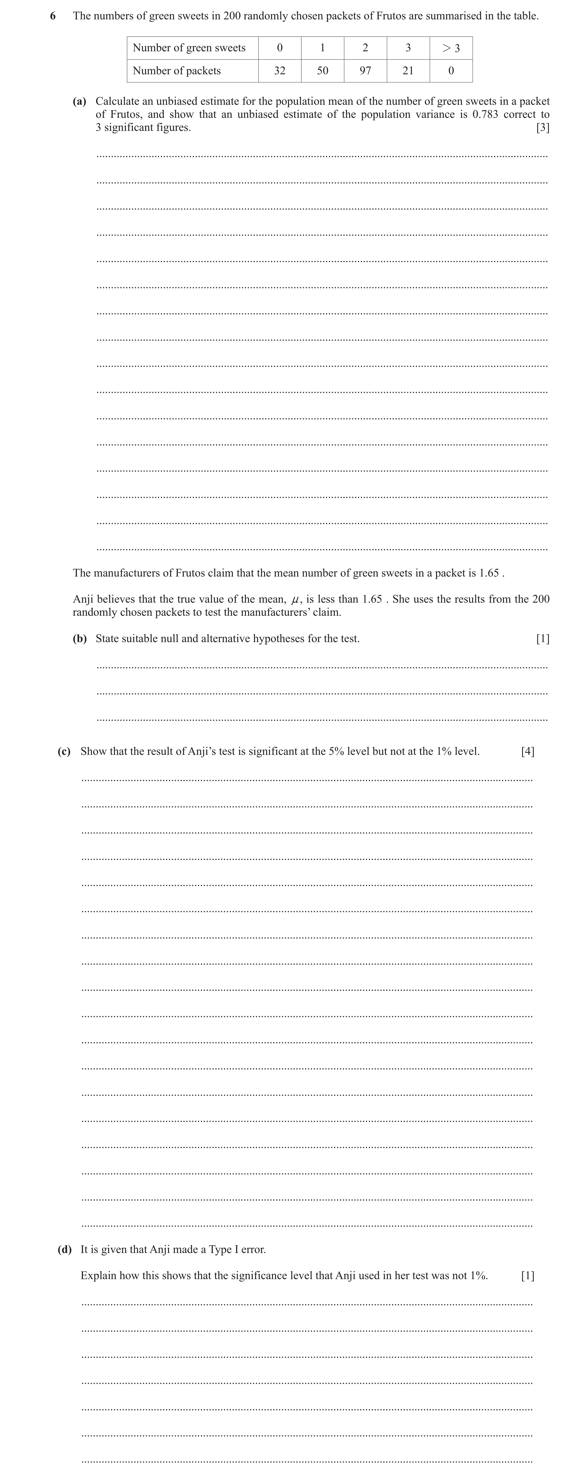
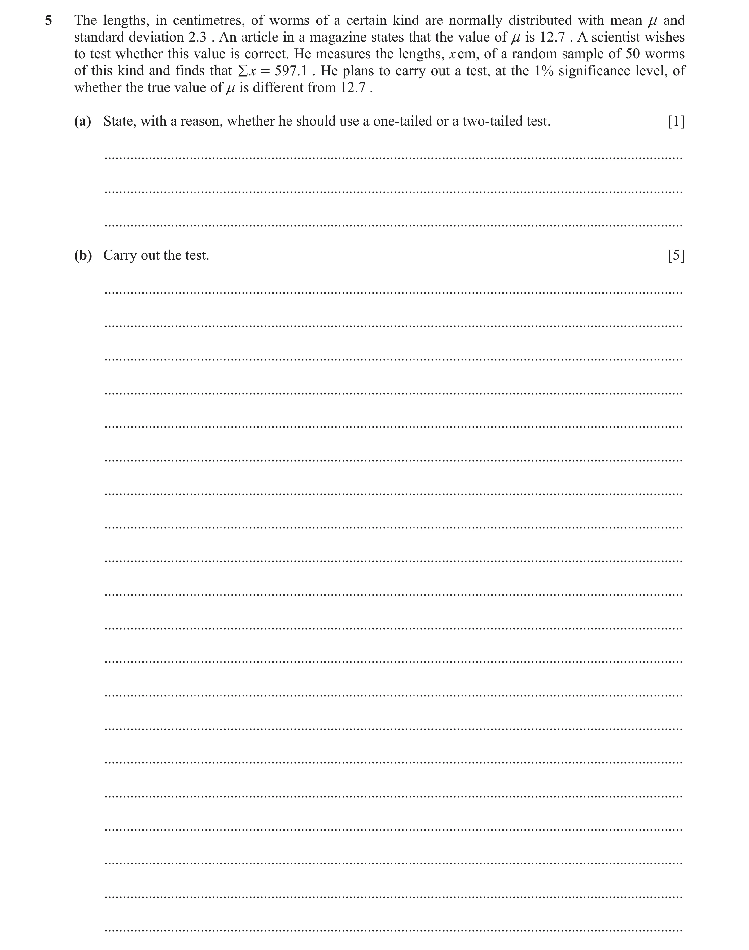 66 / 86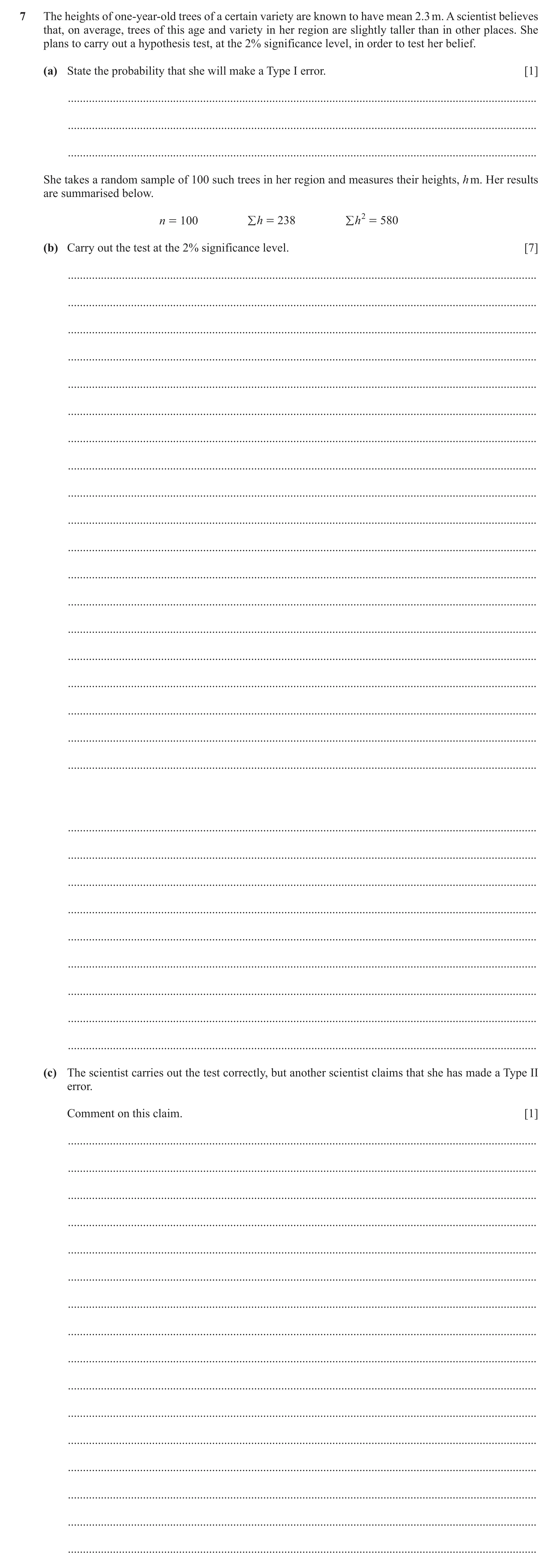
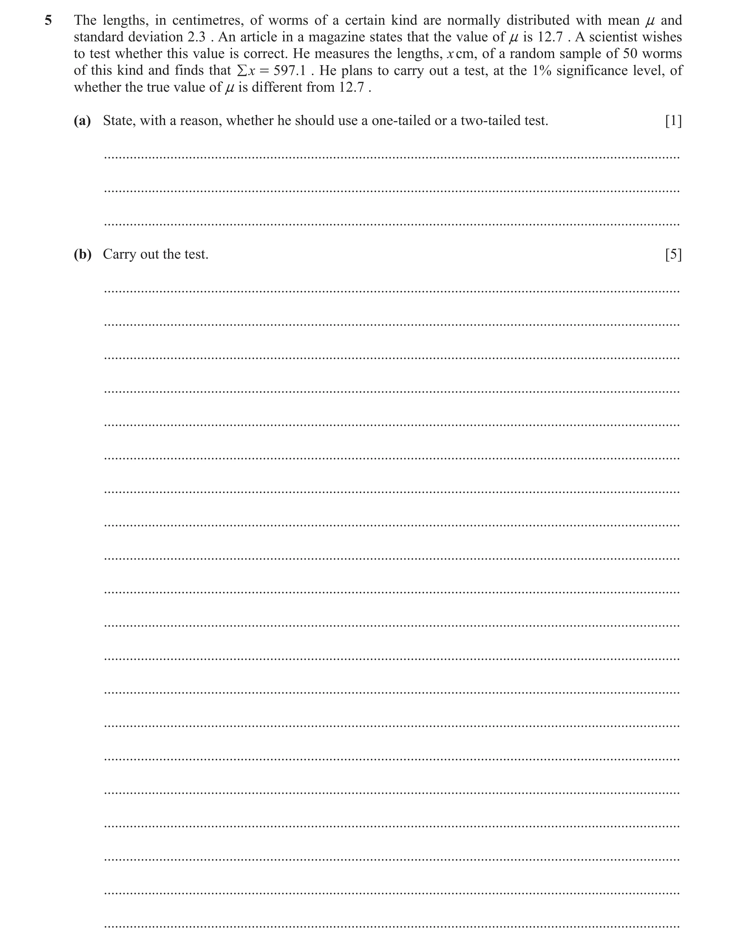 69 / 86
 76 / 86
 79 / 86
 82 / 86
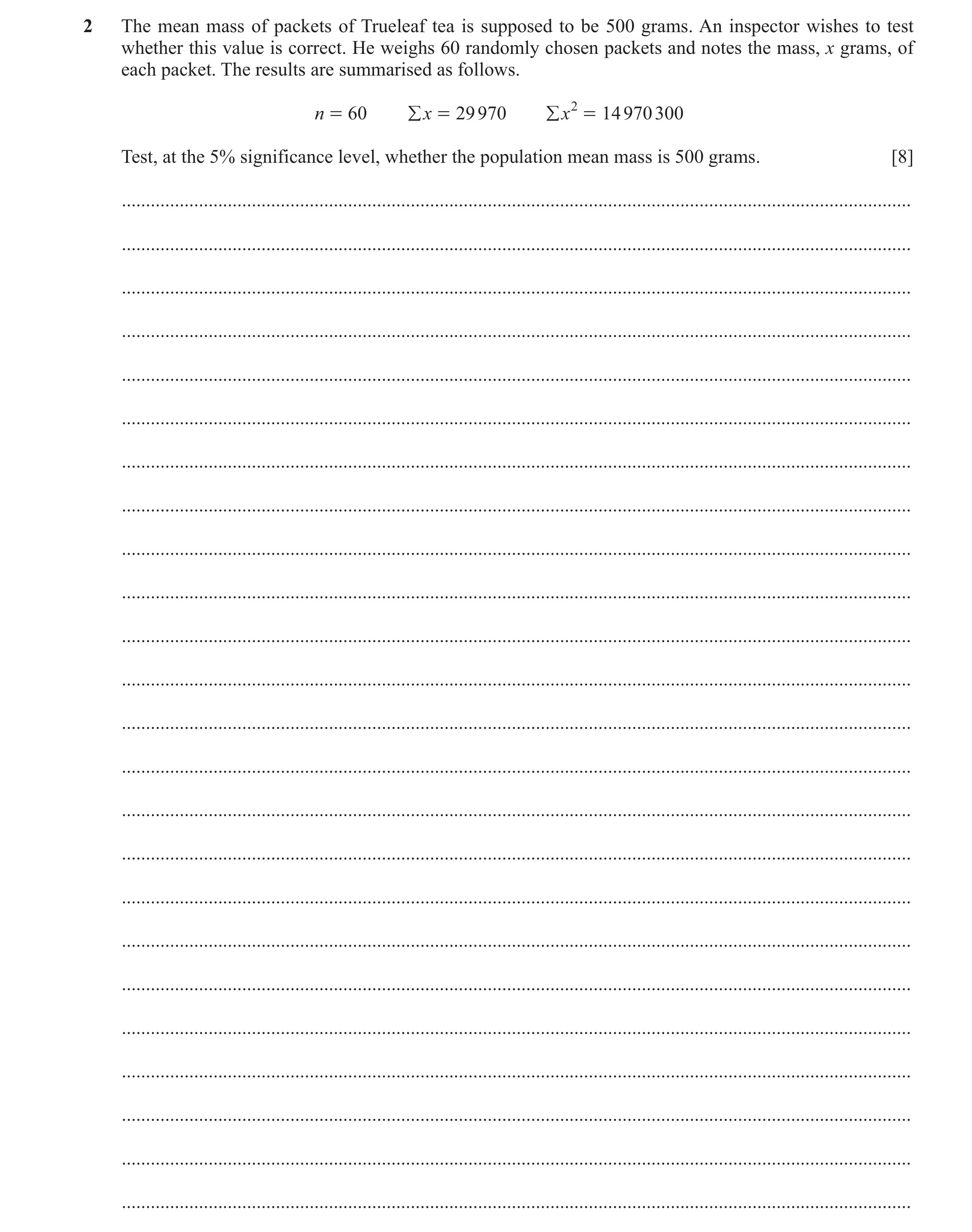 83 / 86
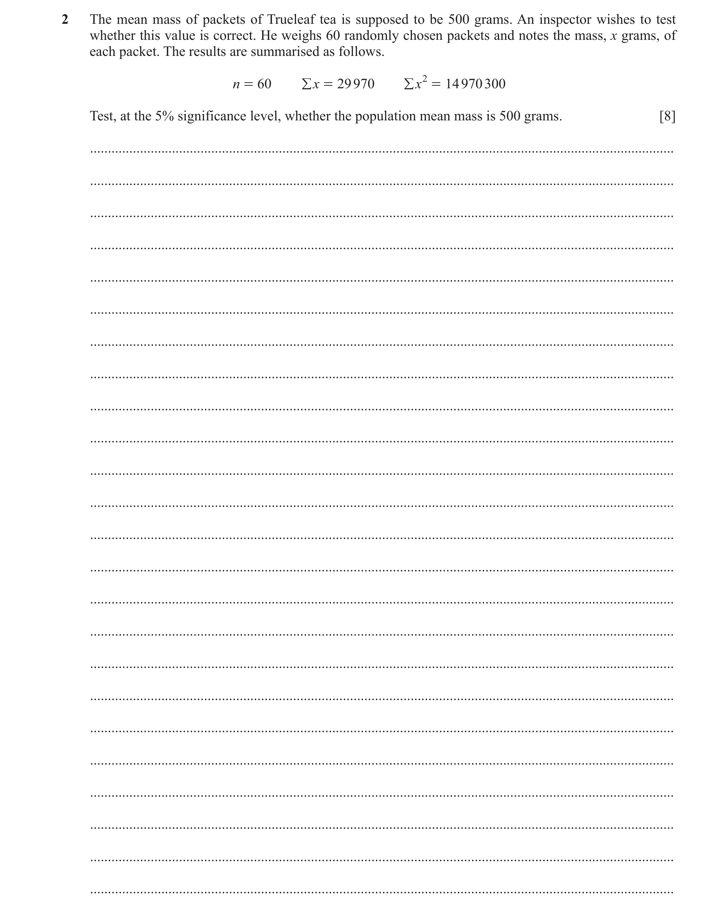 84 / 86
 85 / 86
 86 / 86
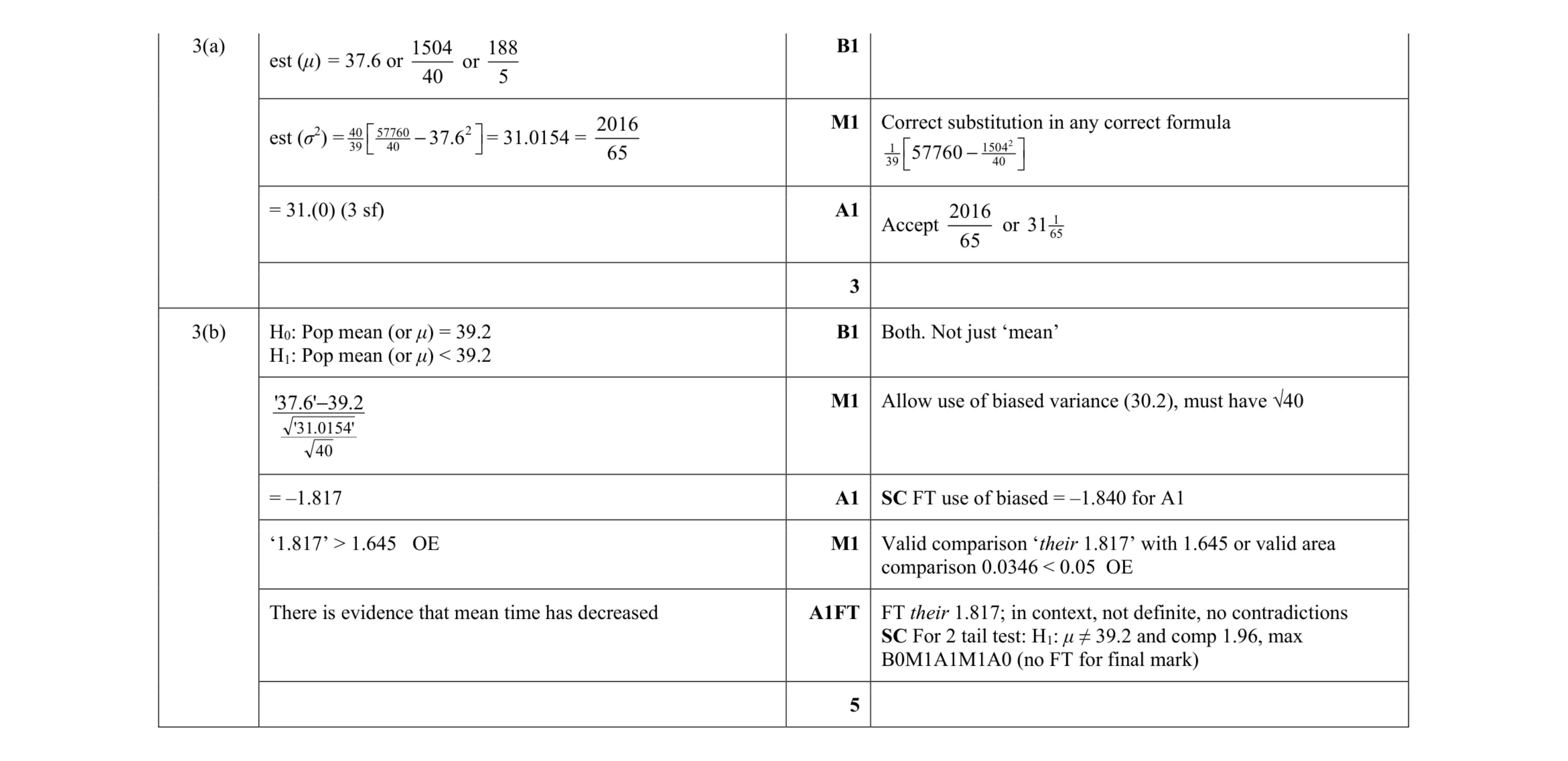 8
8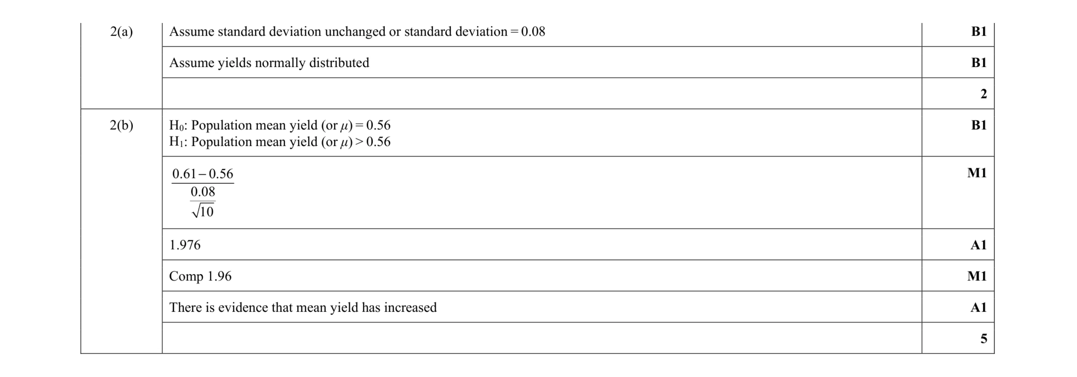 7
7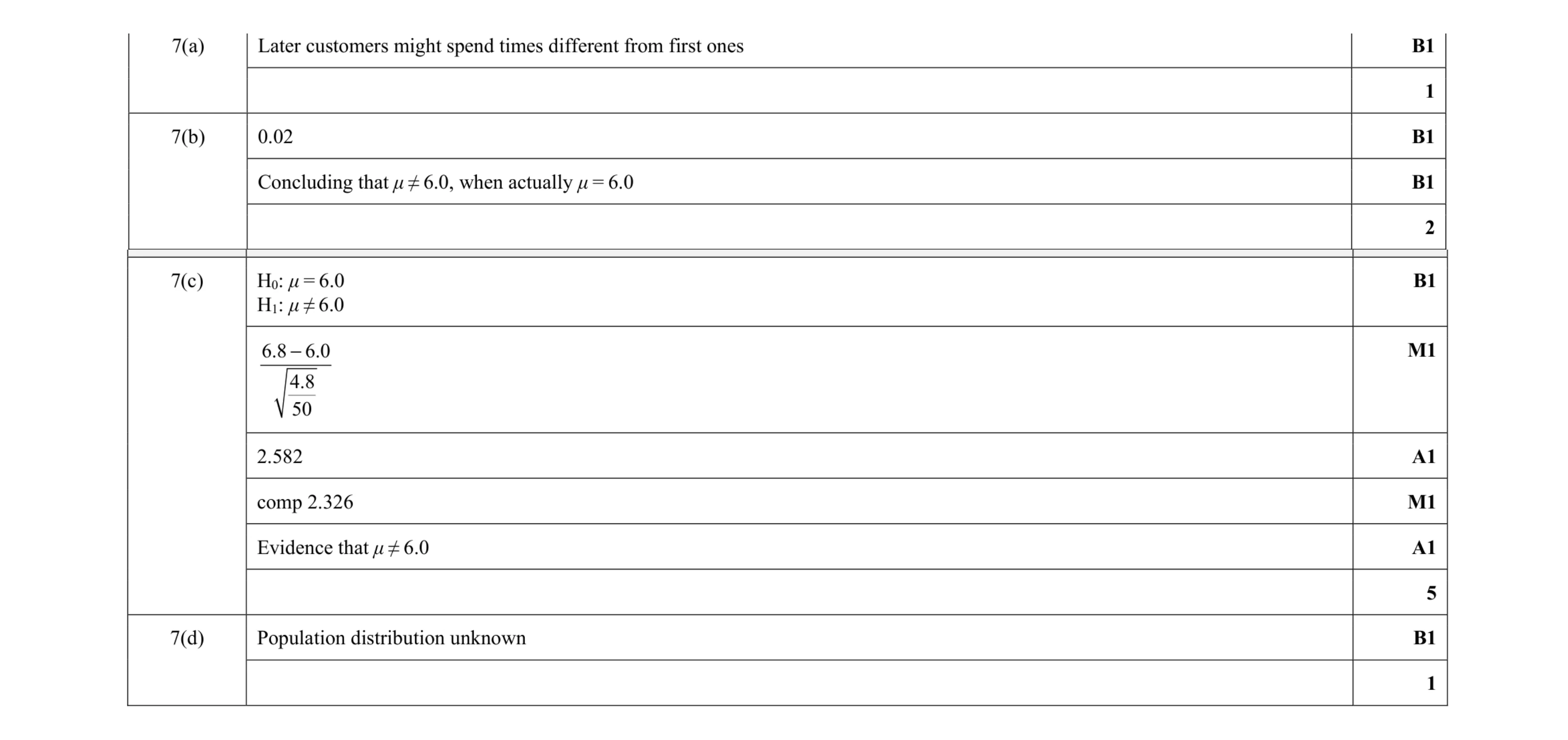 9
9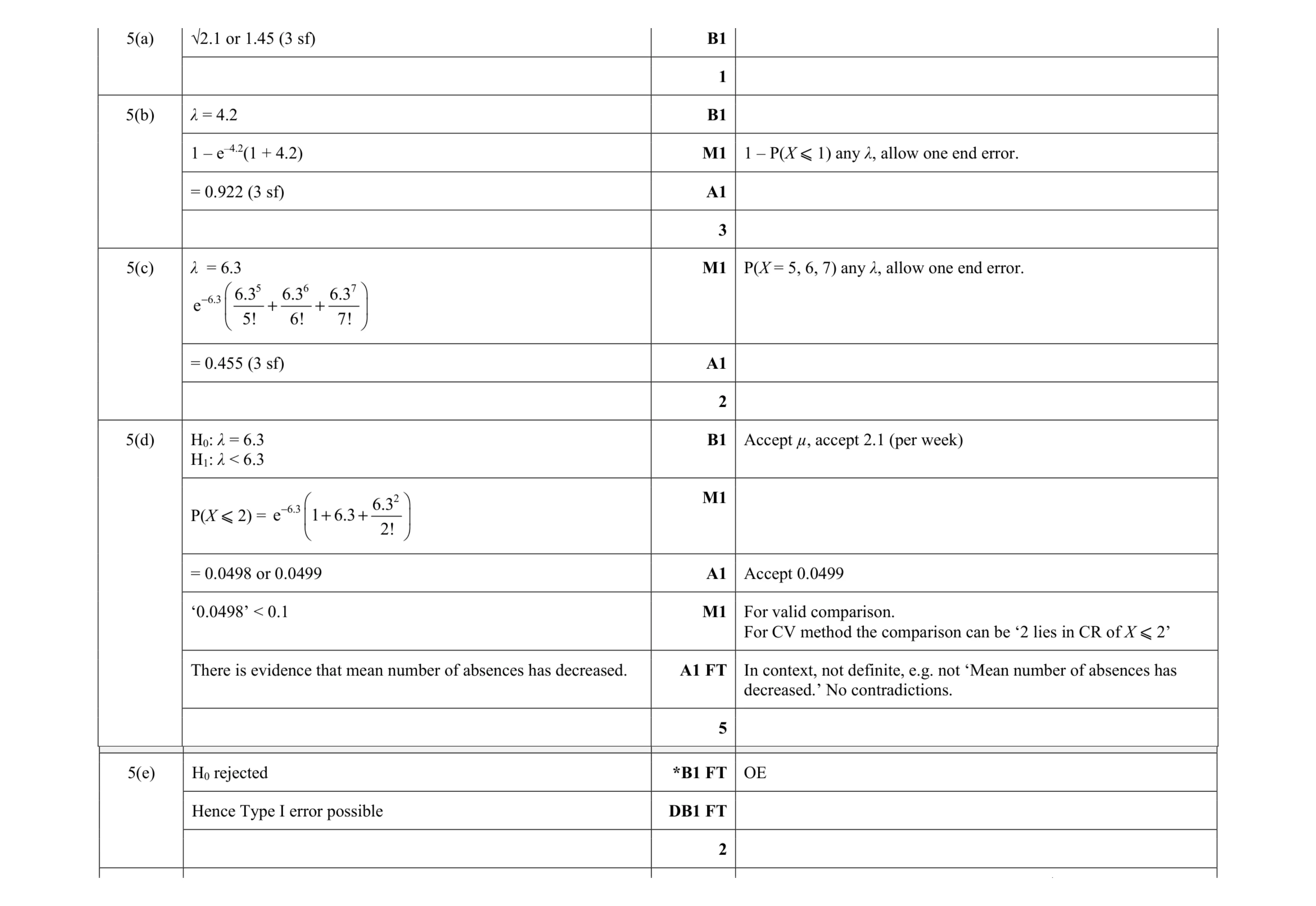 13
13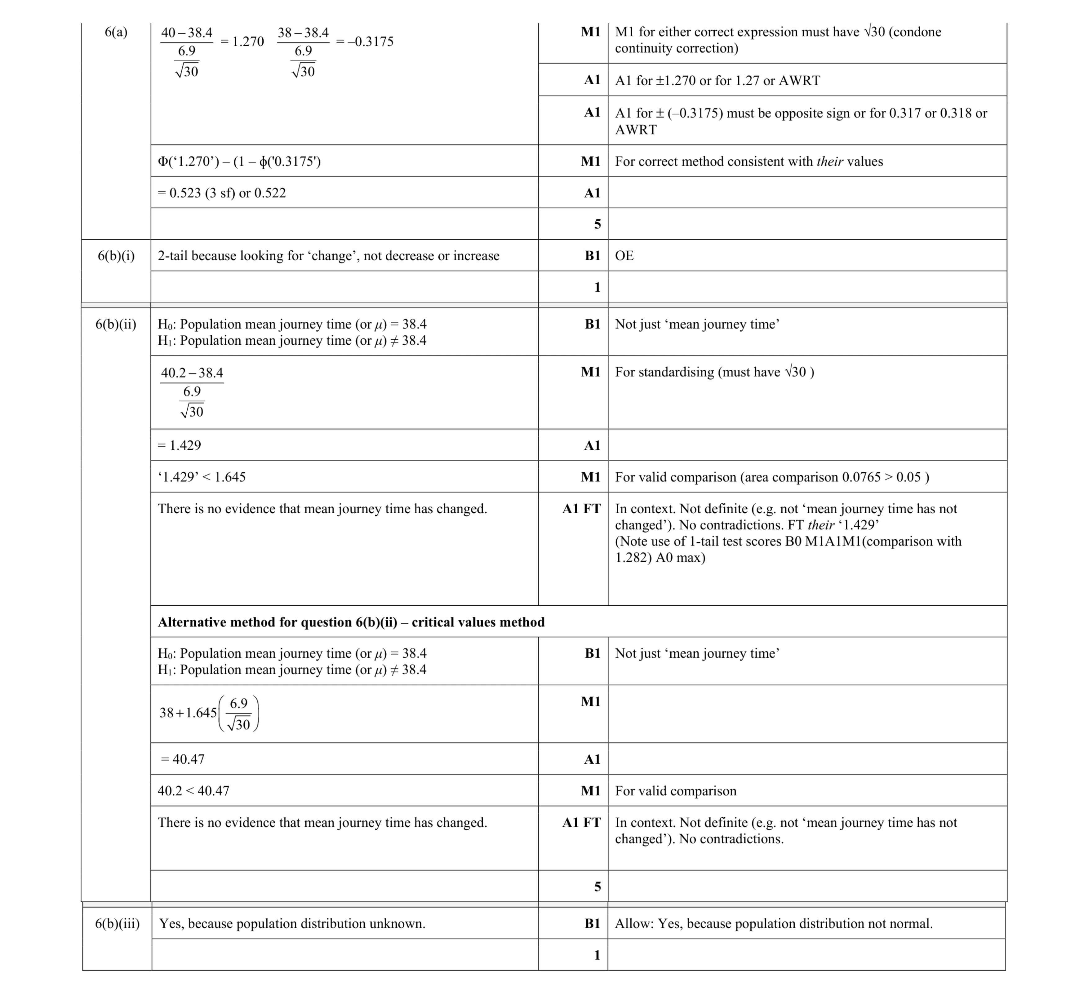 12
12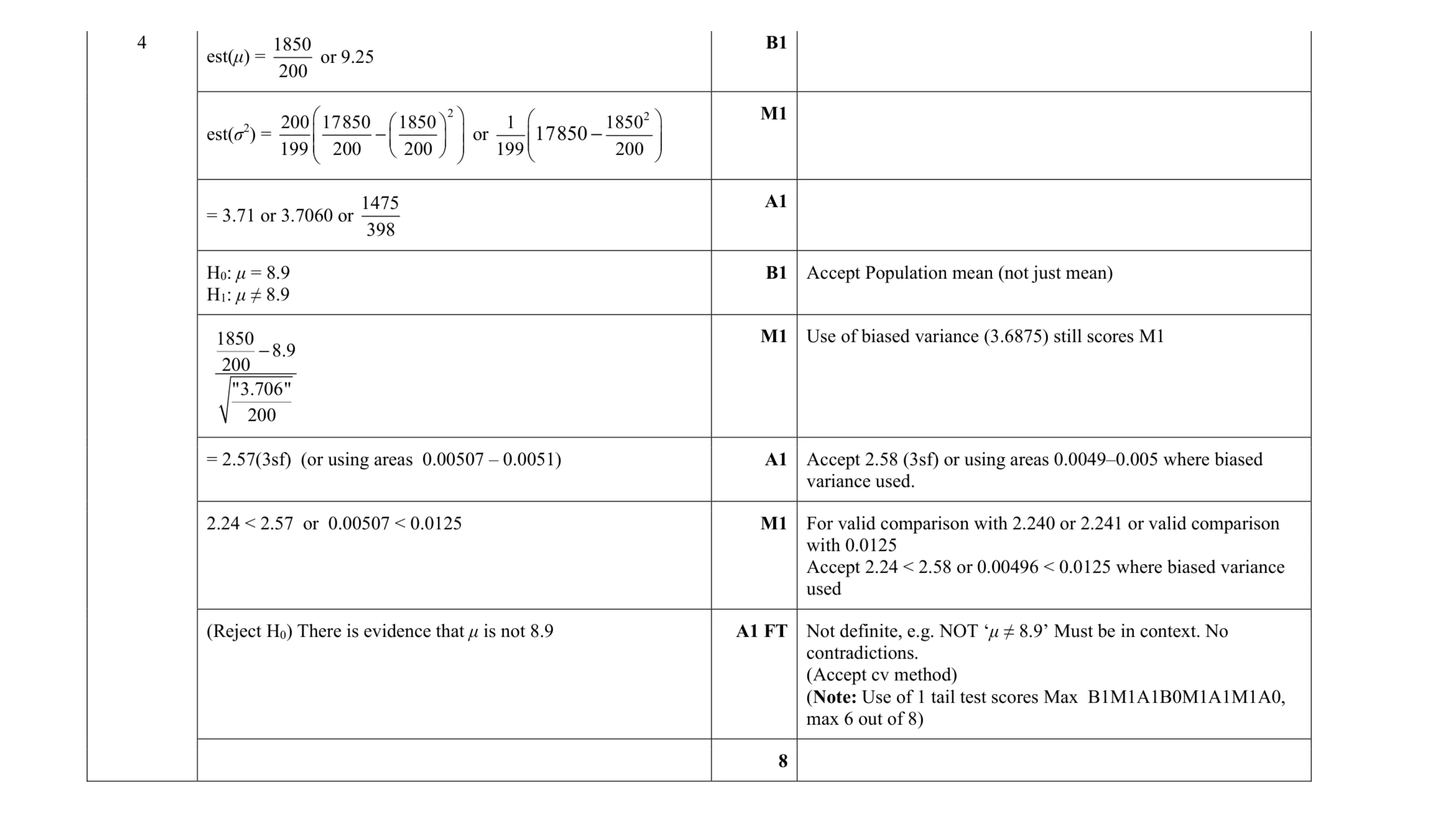 8
8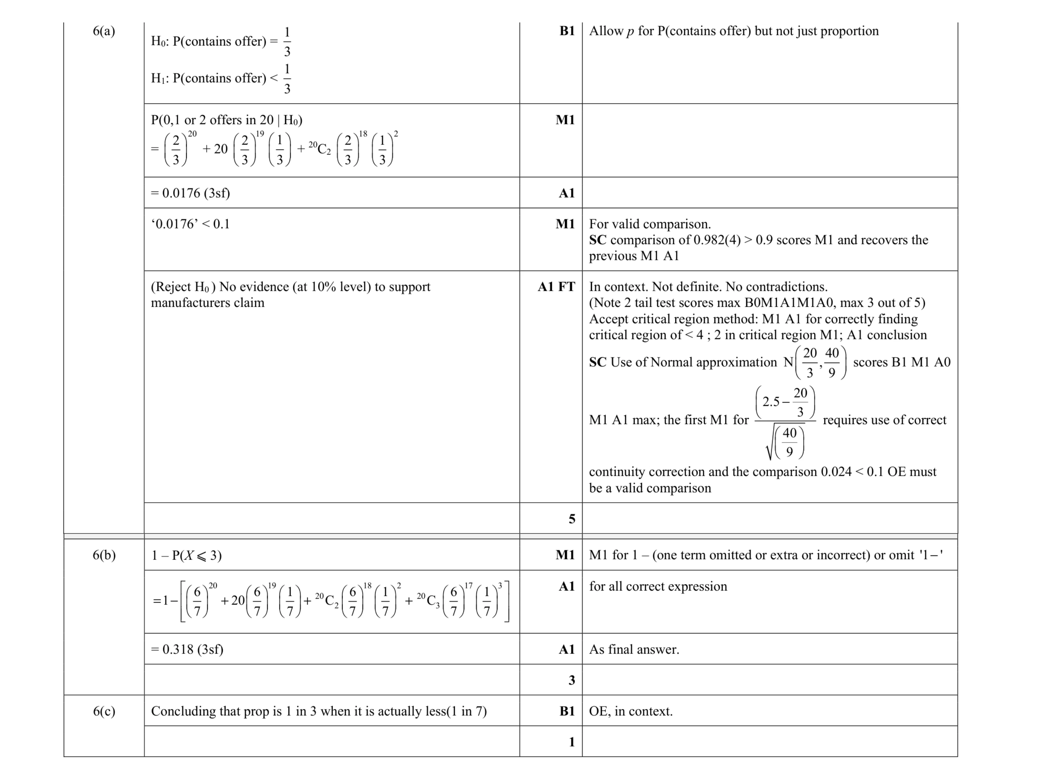 9
9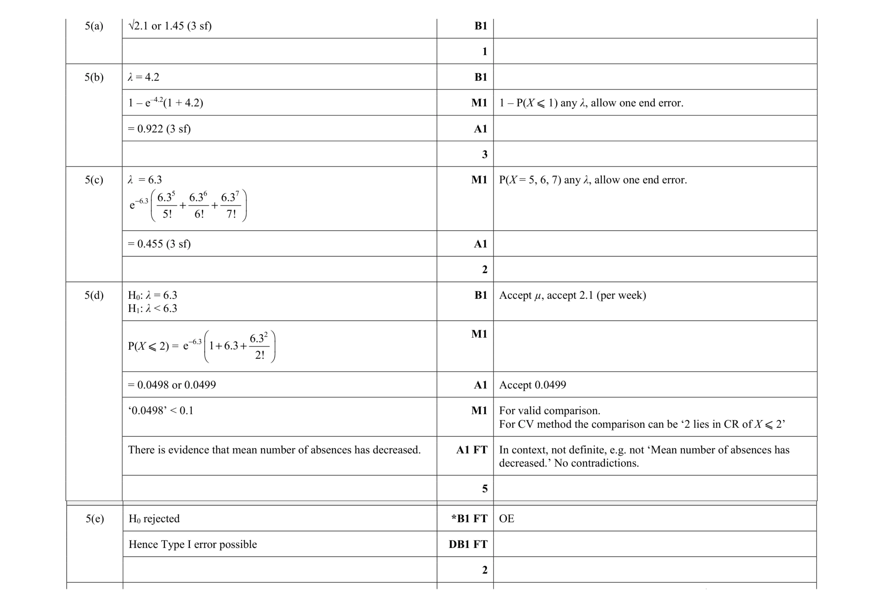 13
13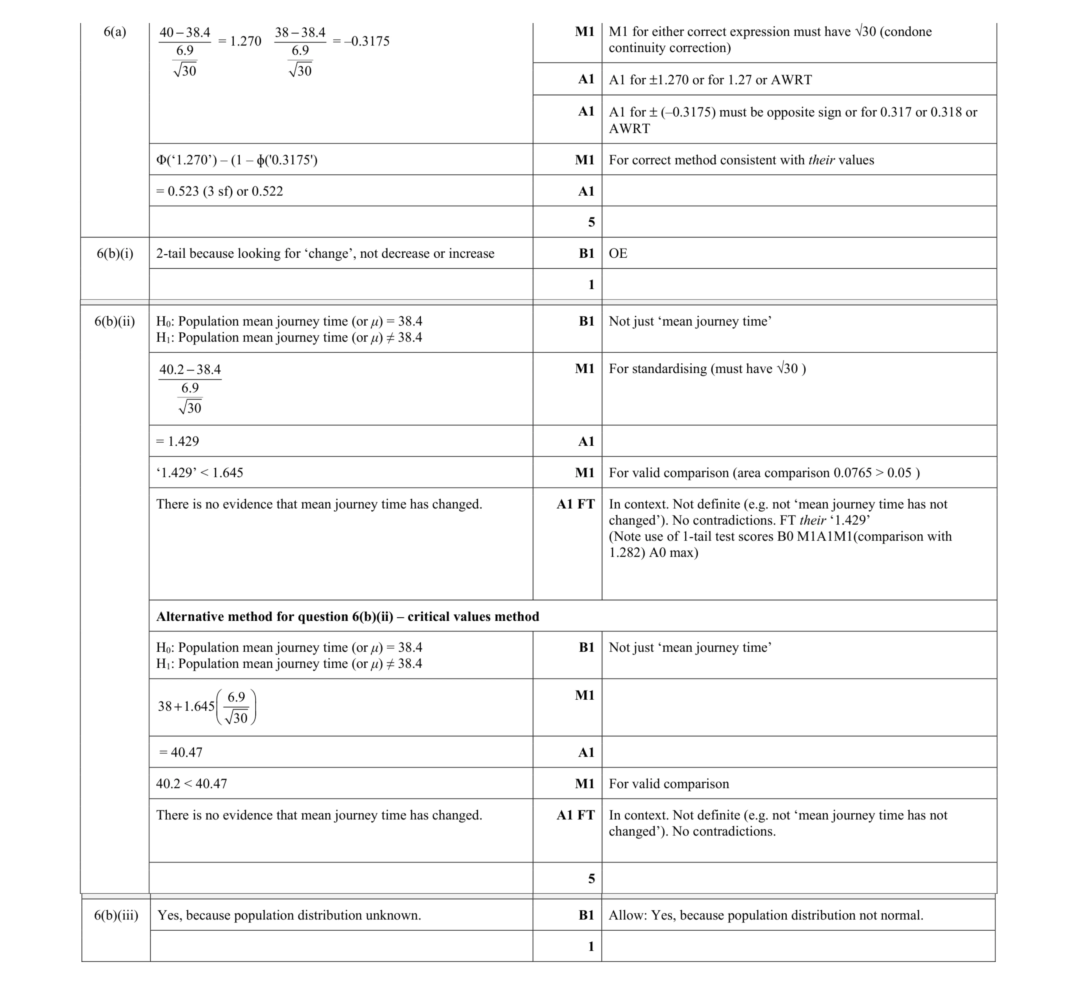 12
12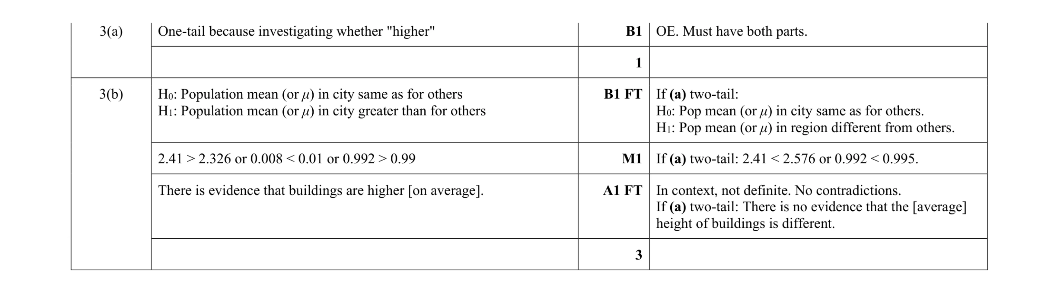 4
4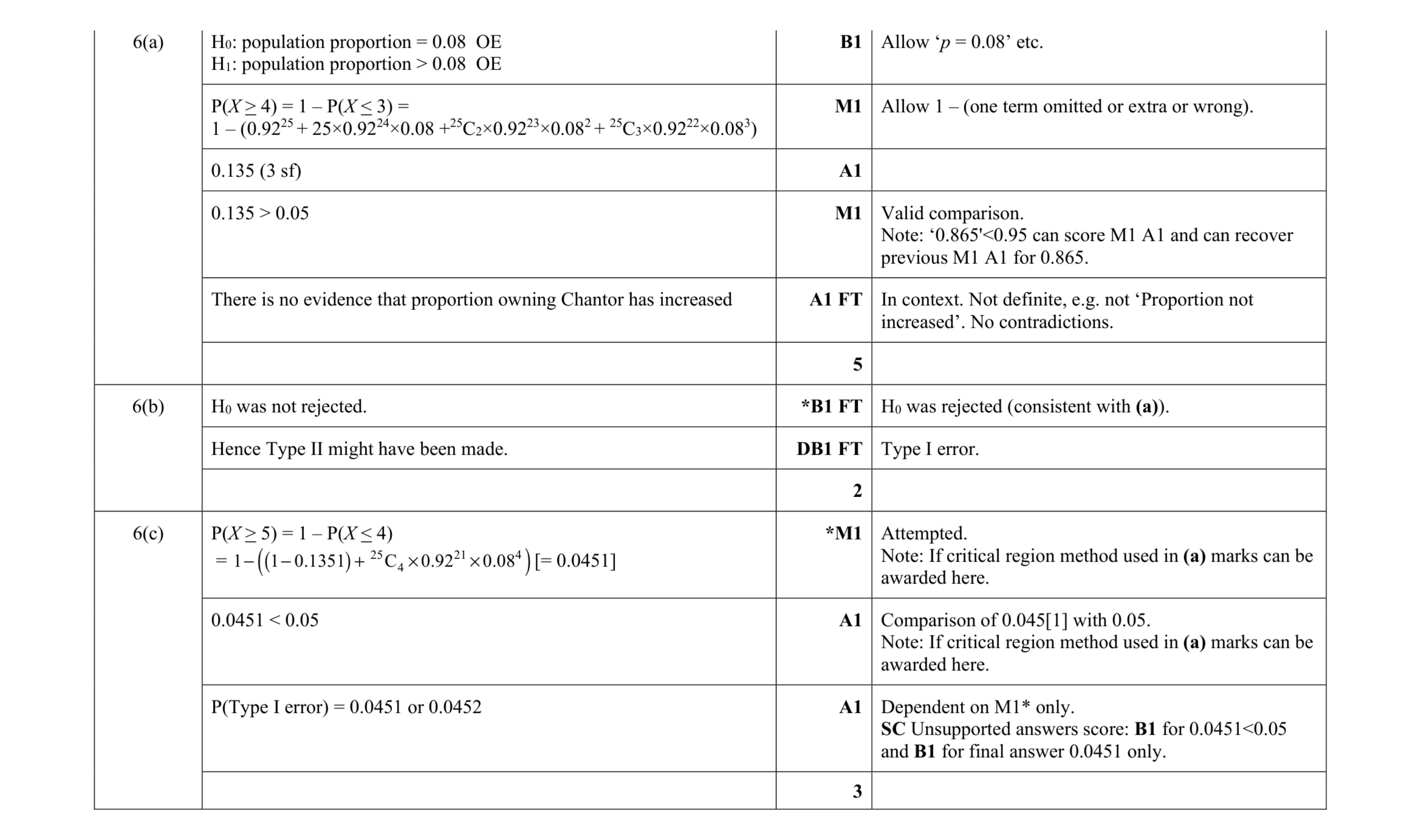 10
10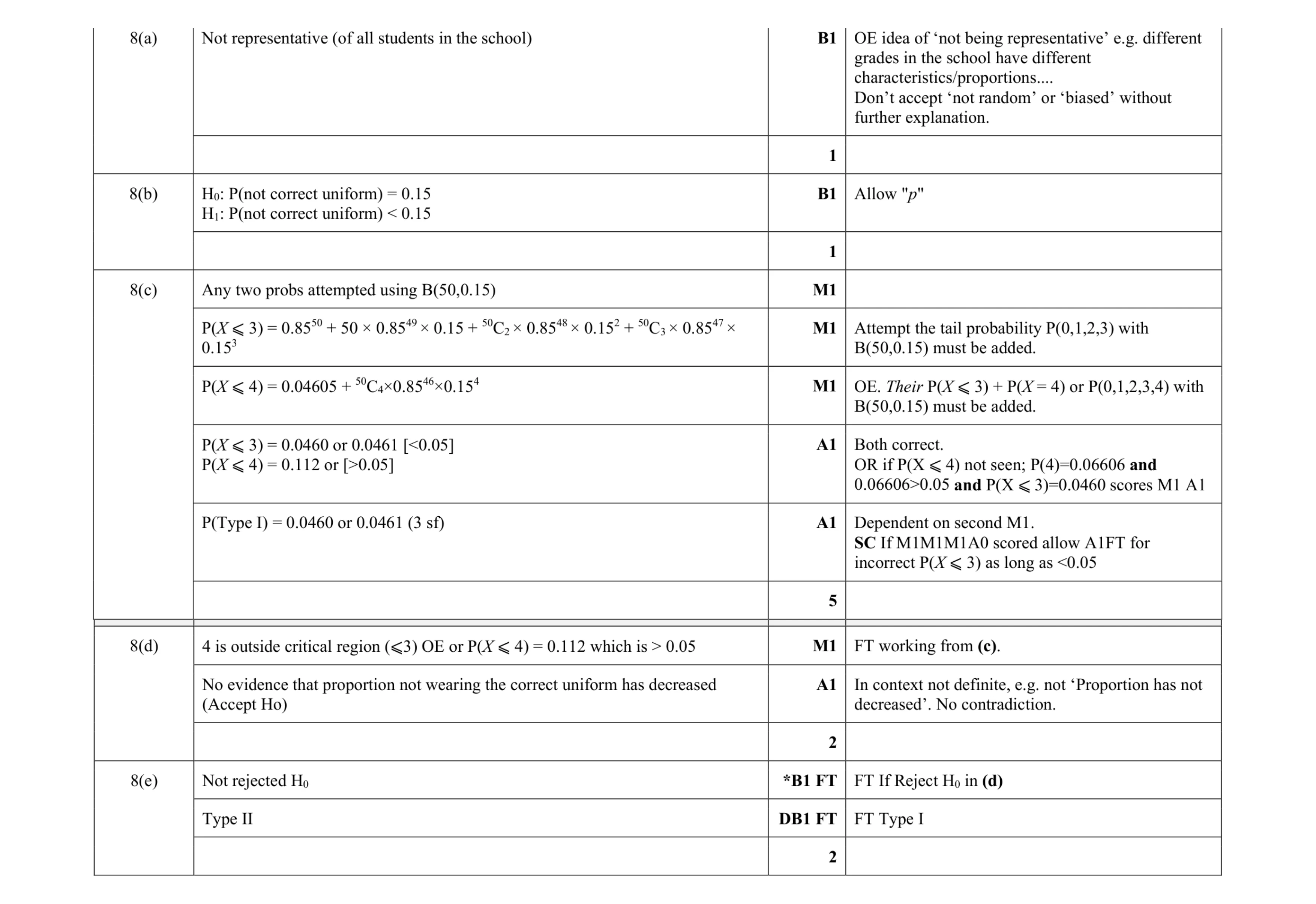 11
11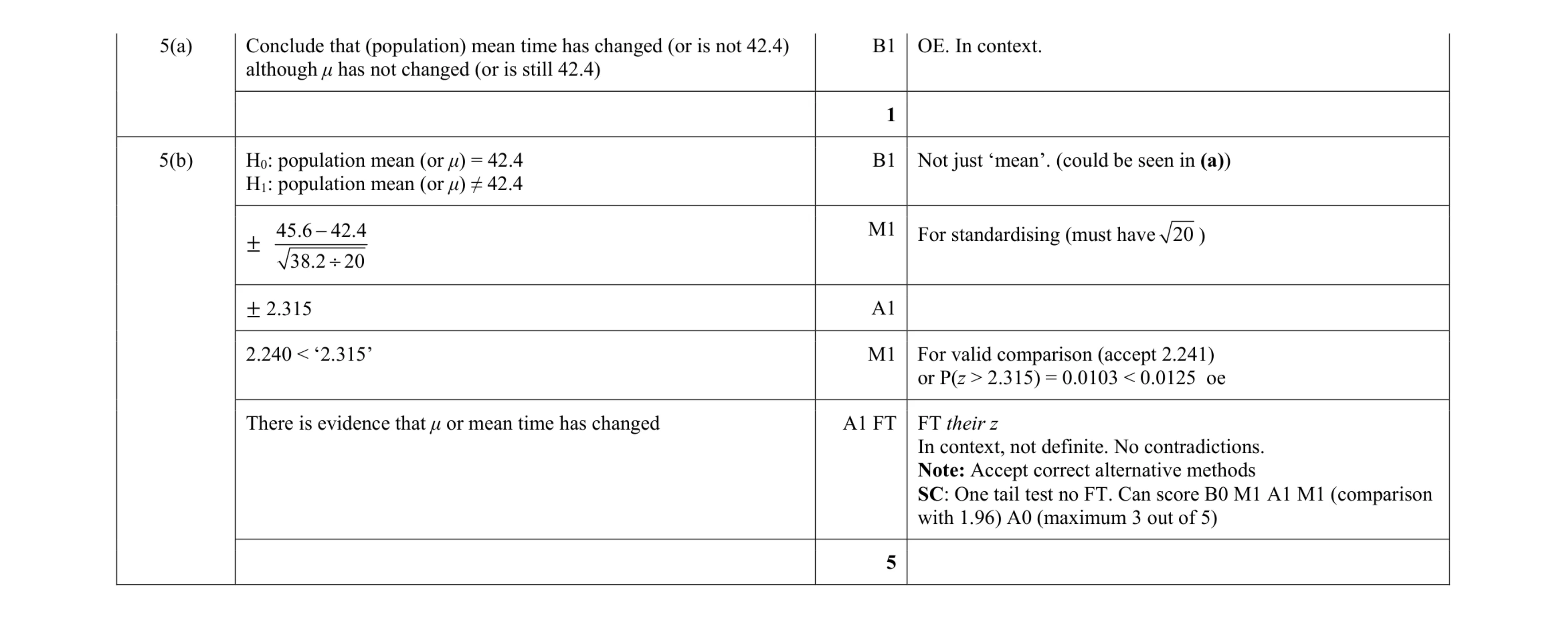 6
6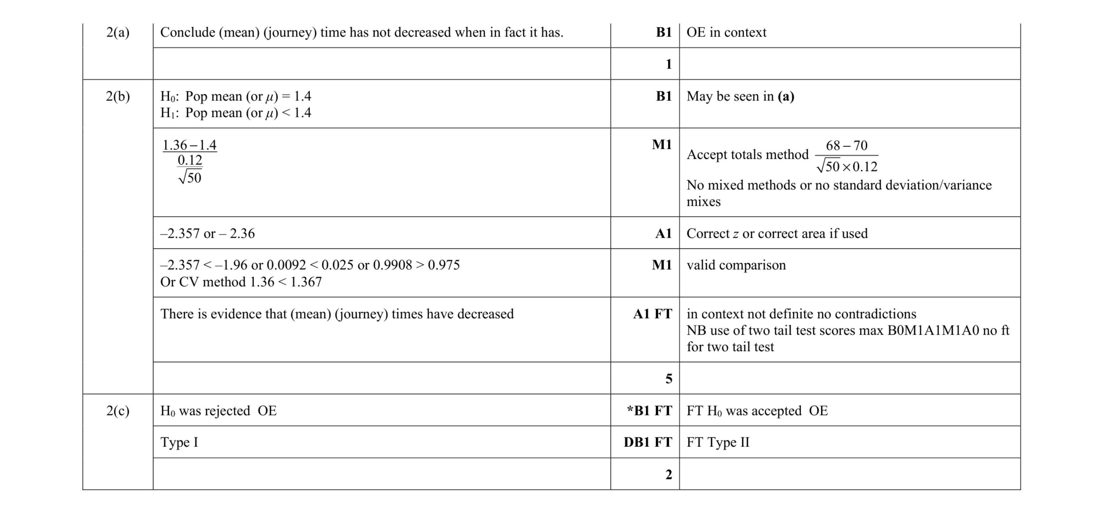 8
8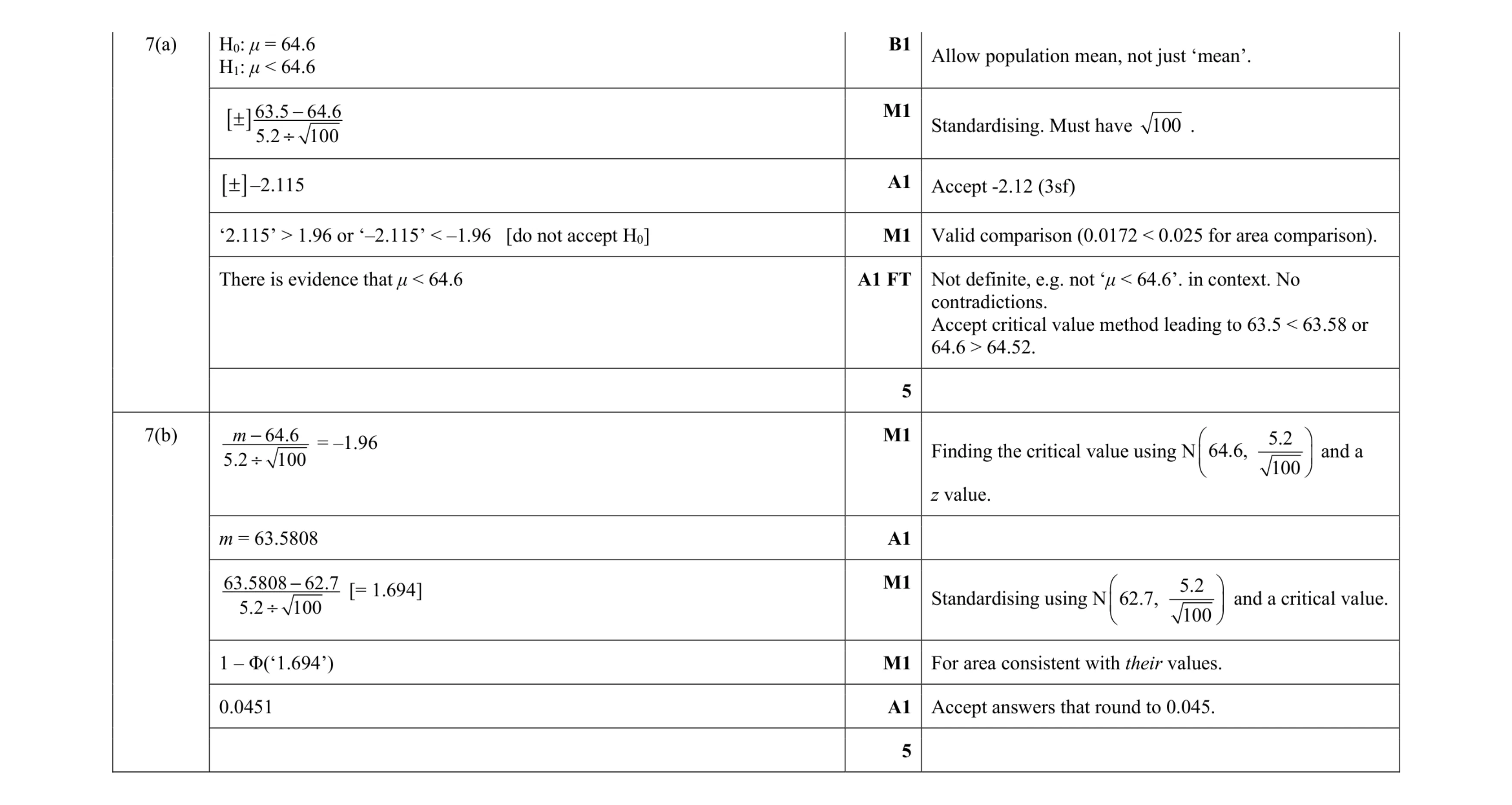 10
10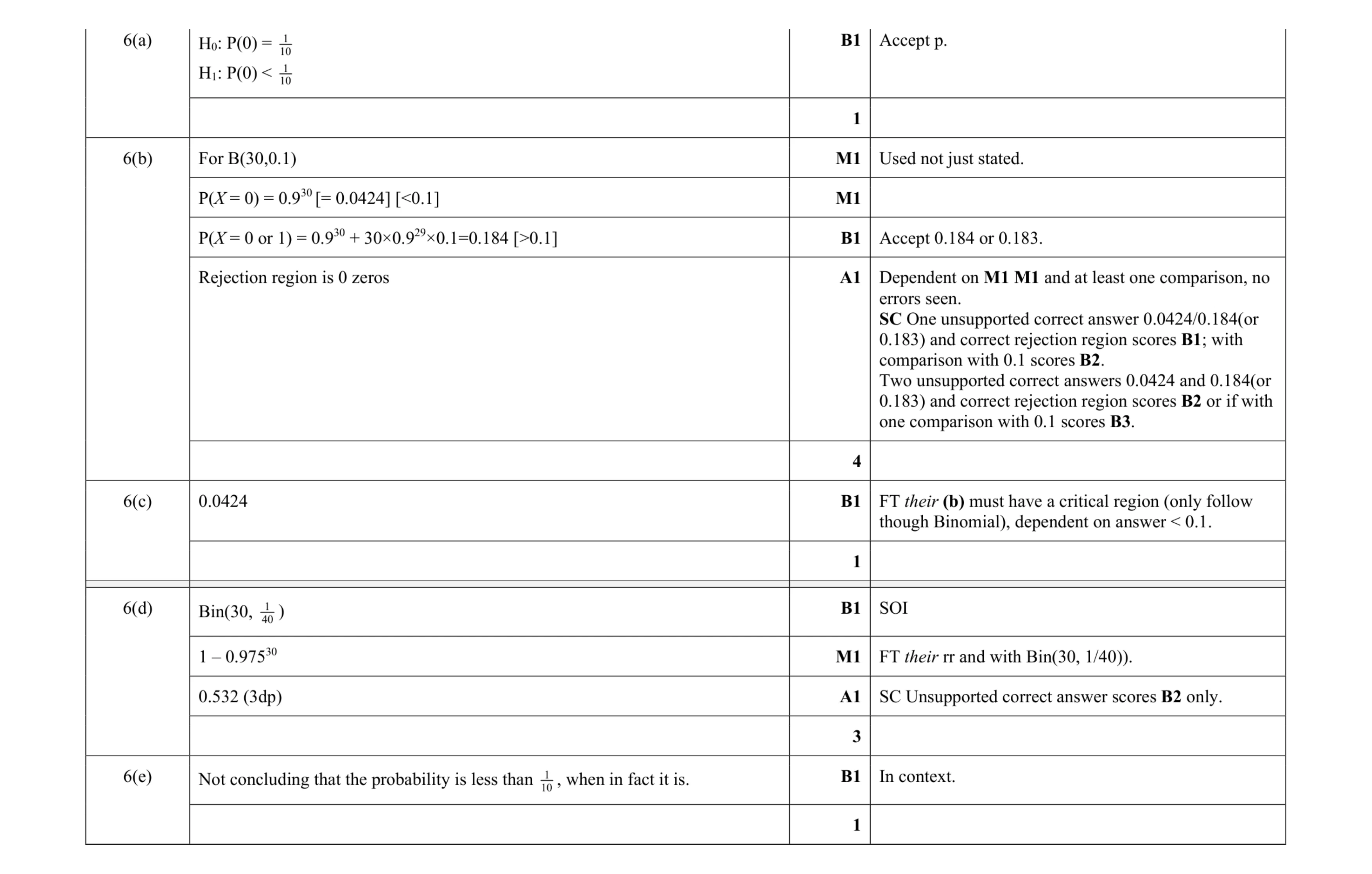 10
10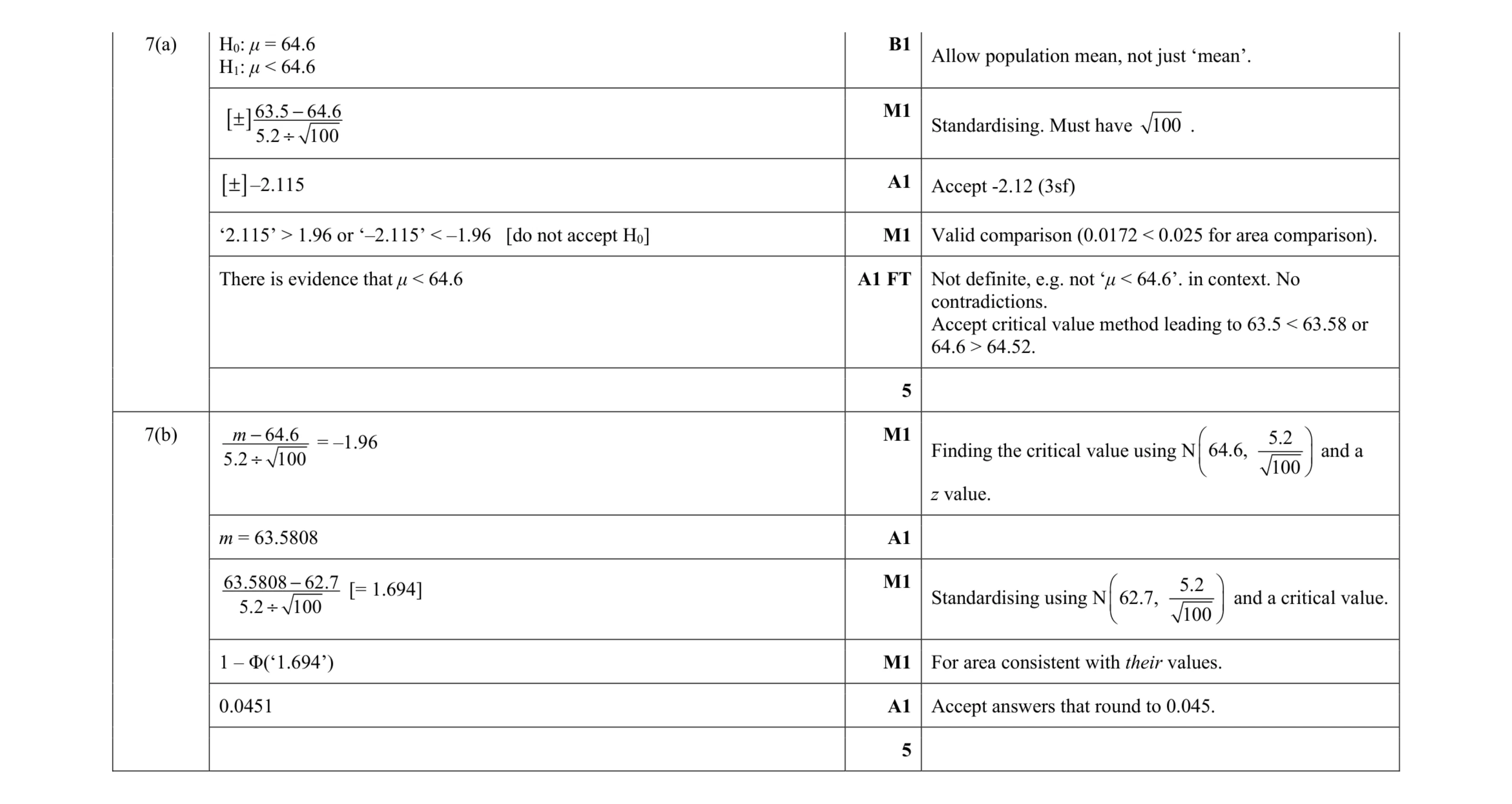 10
10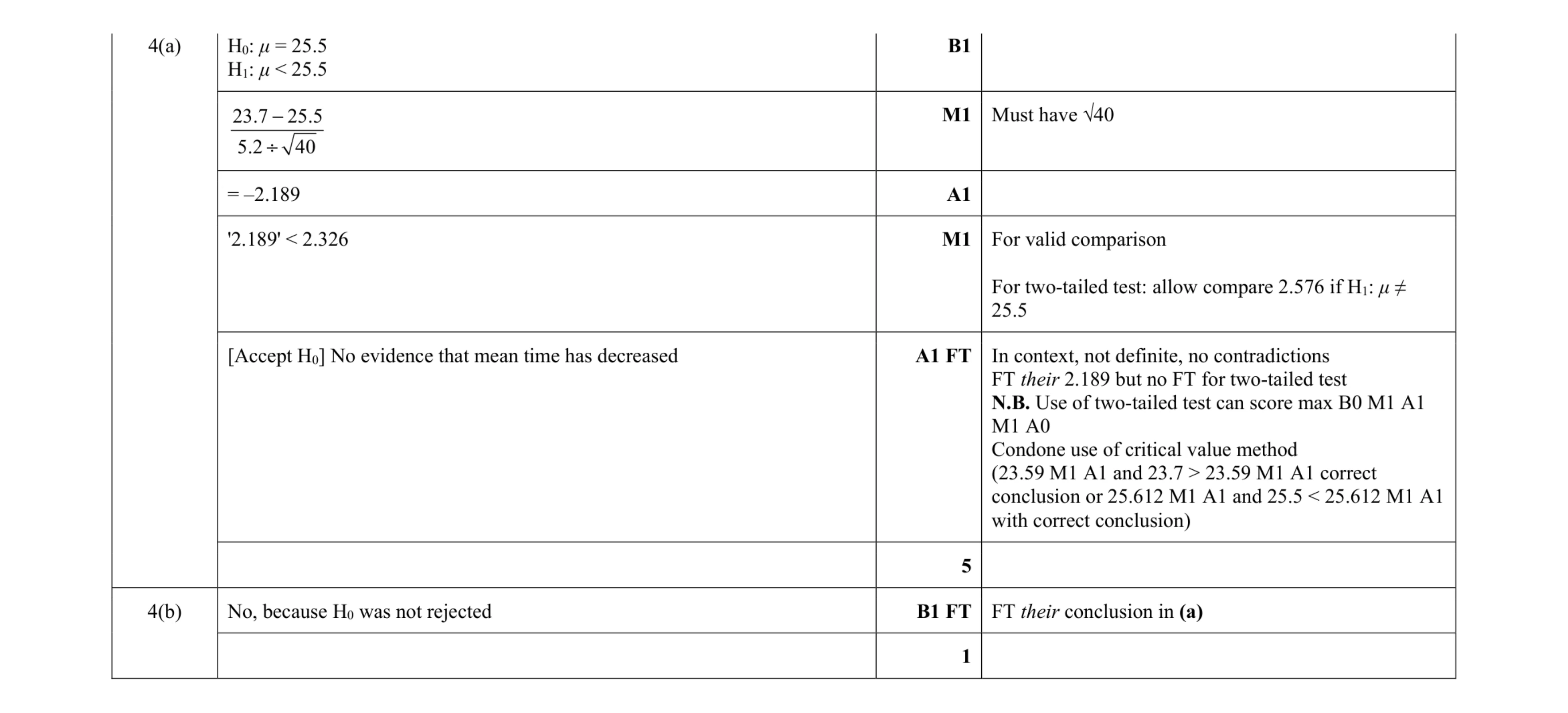 6
6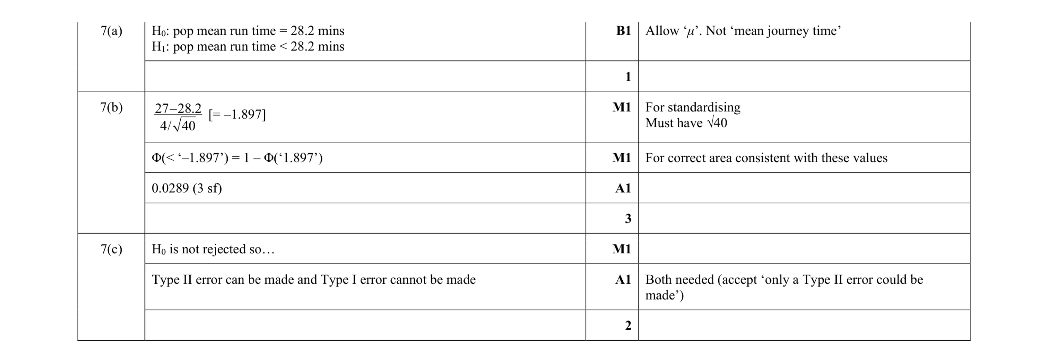 6
6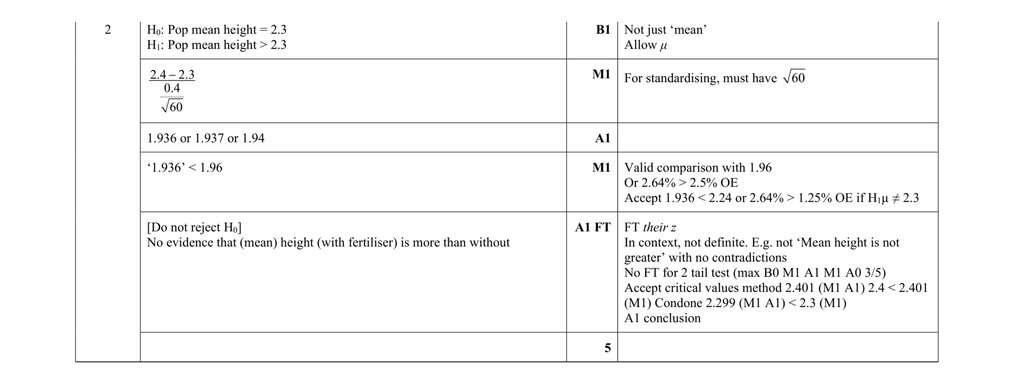 5
5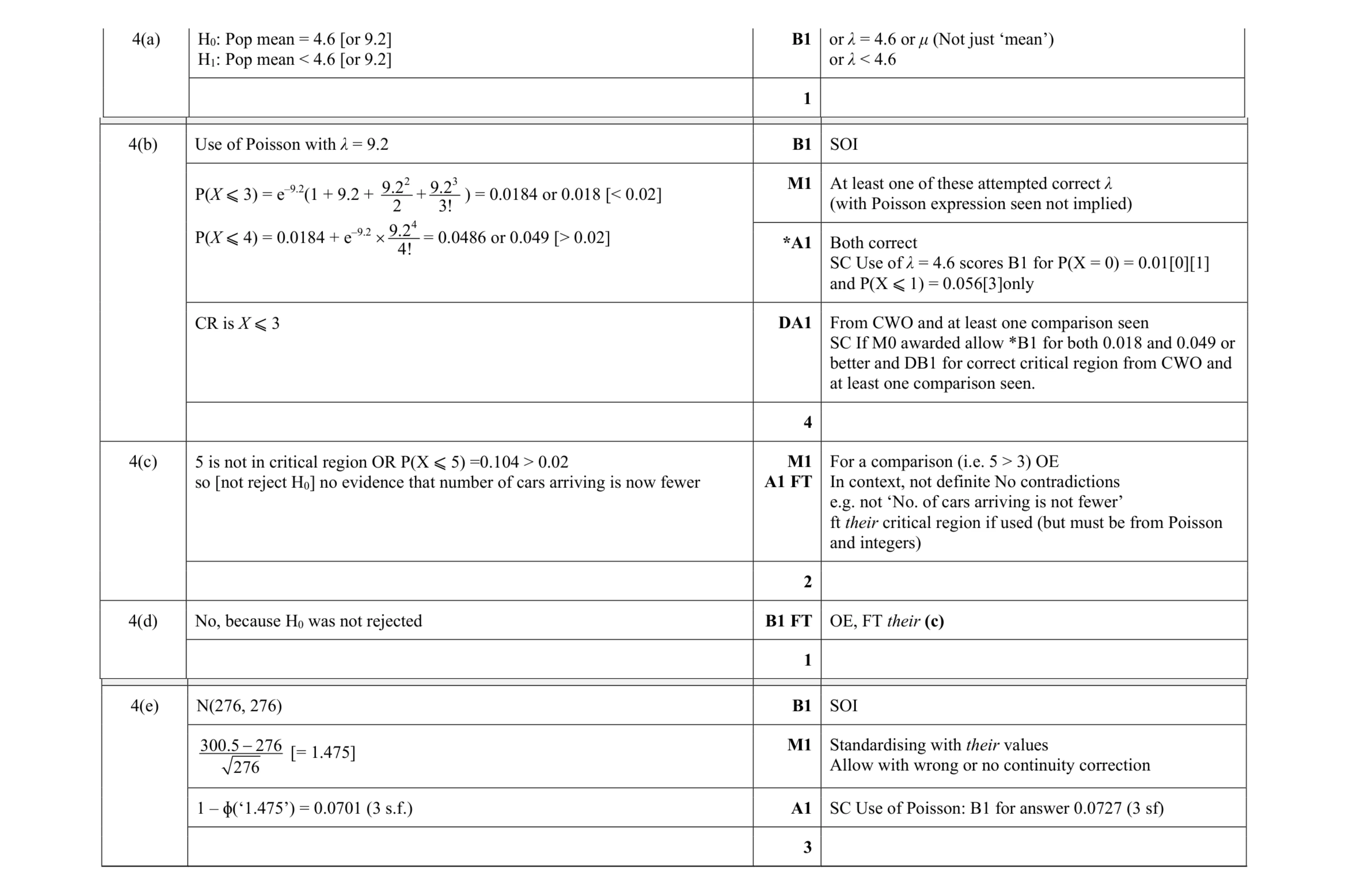 5
5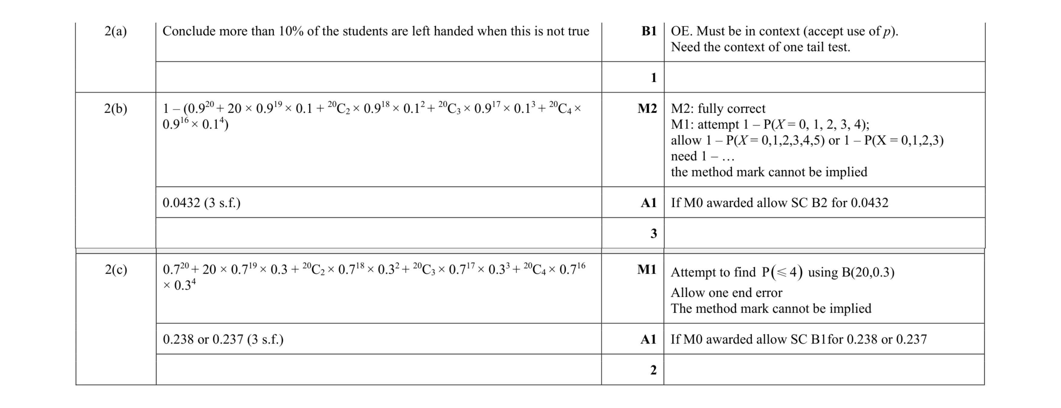 6
6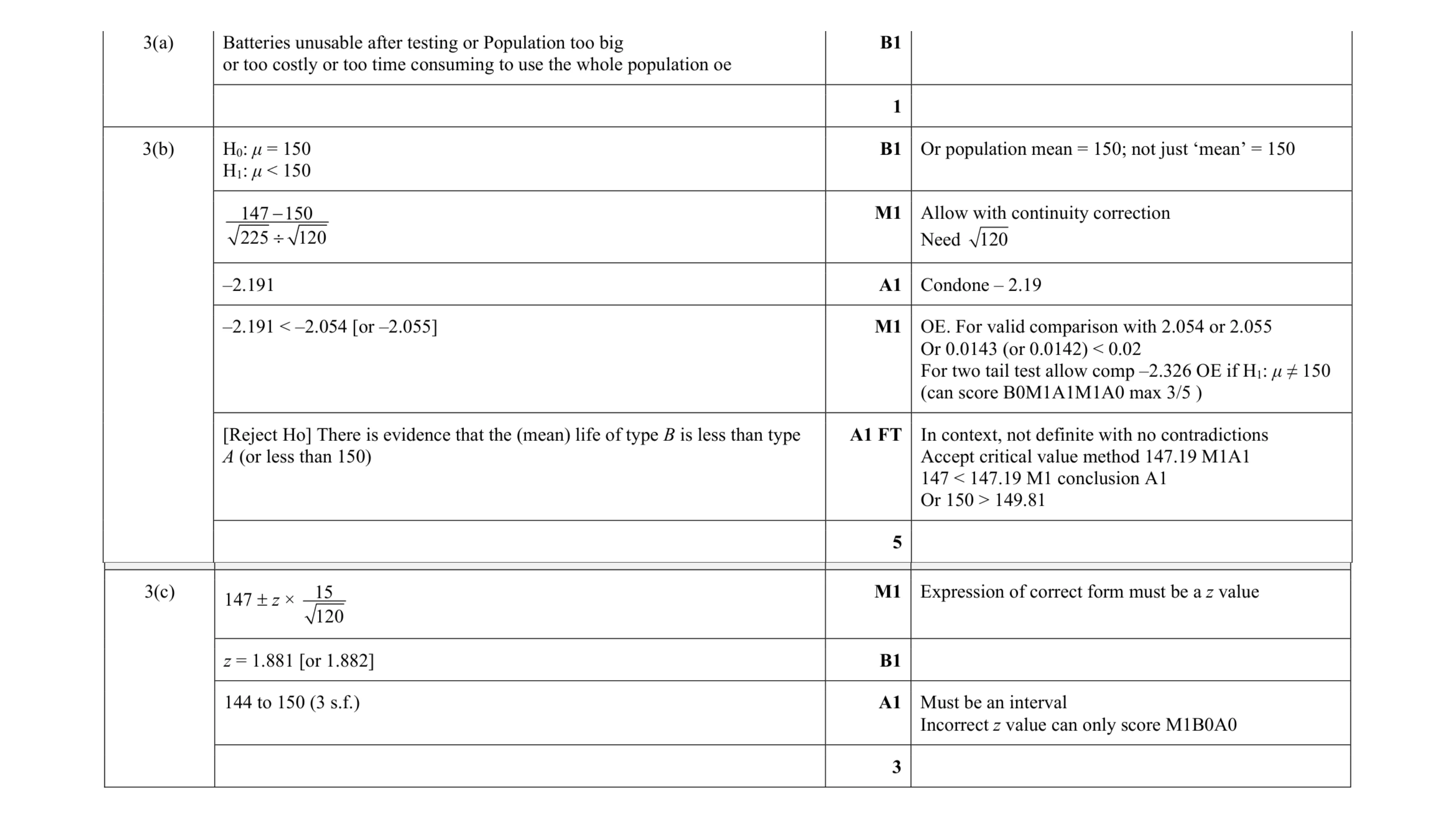 9
9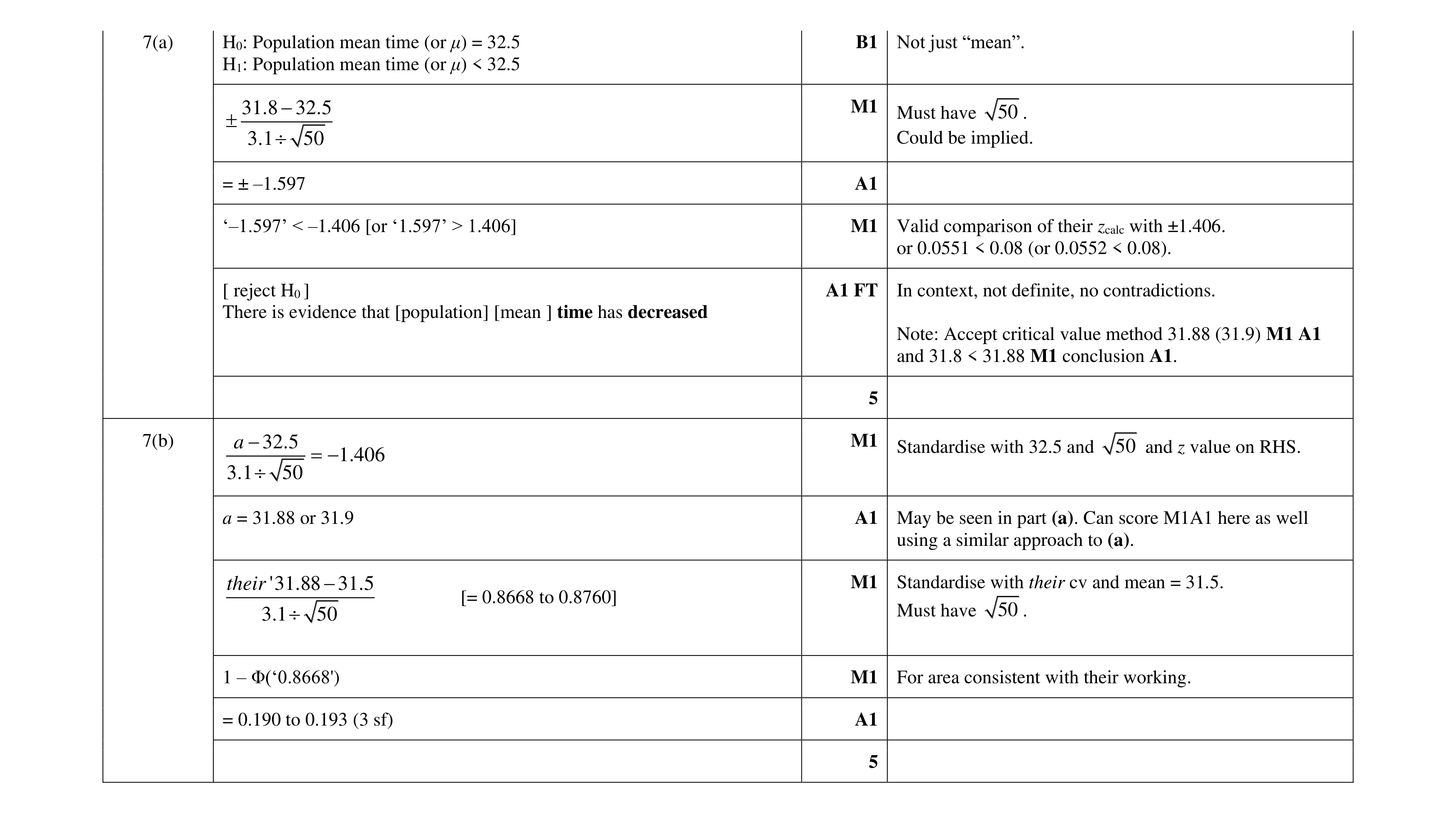 10
10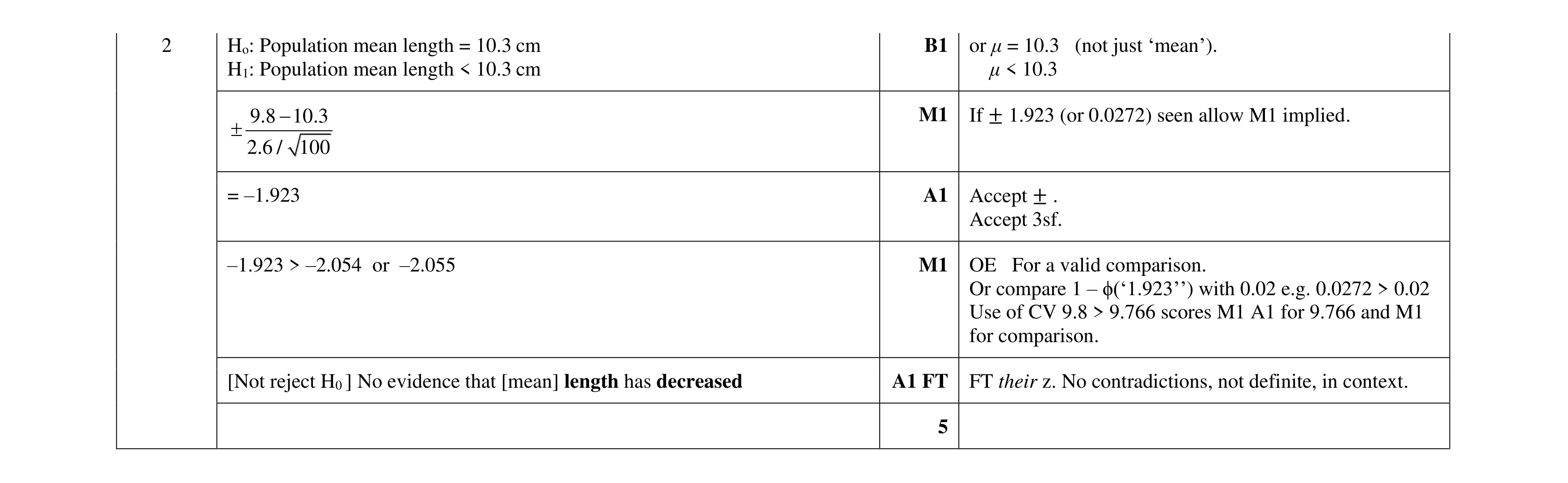 5
5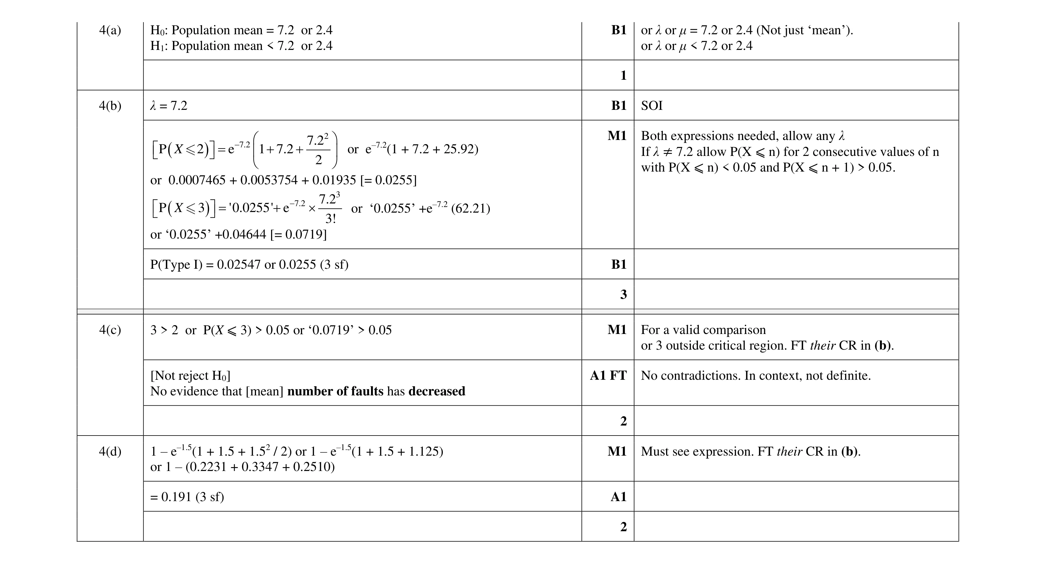 8
8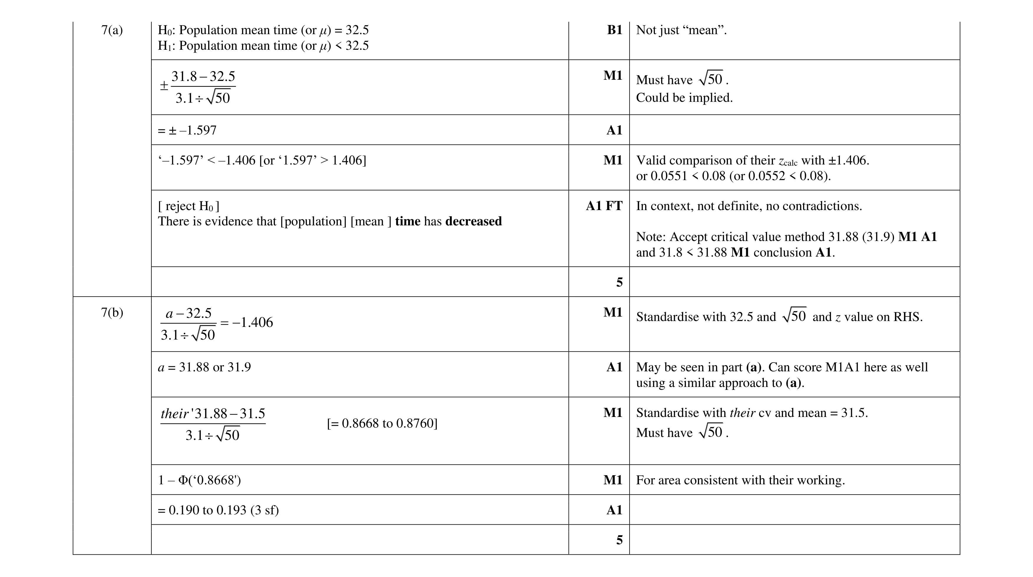 10
10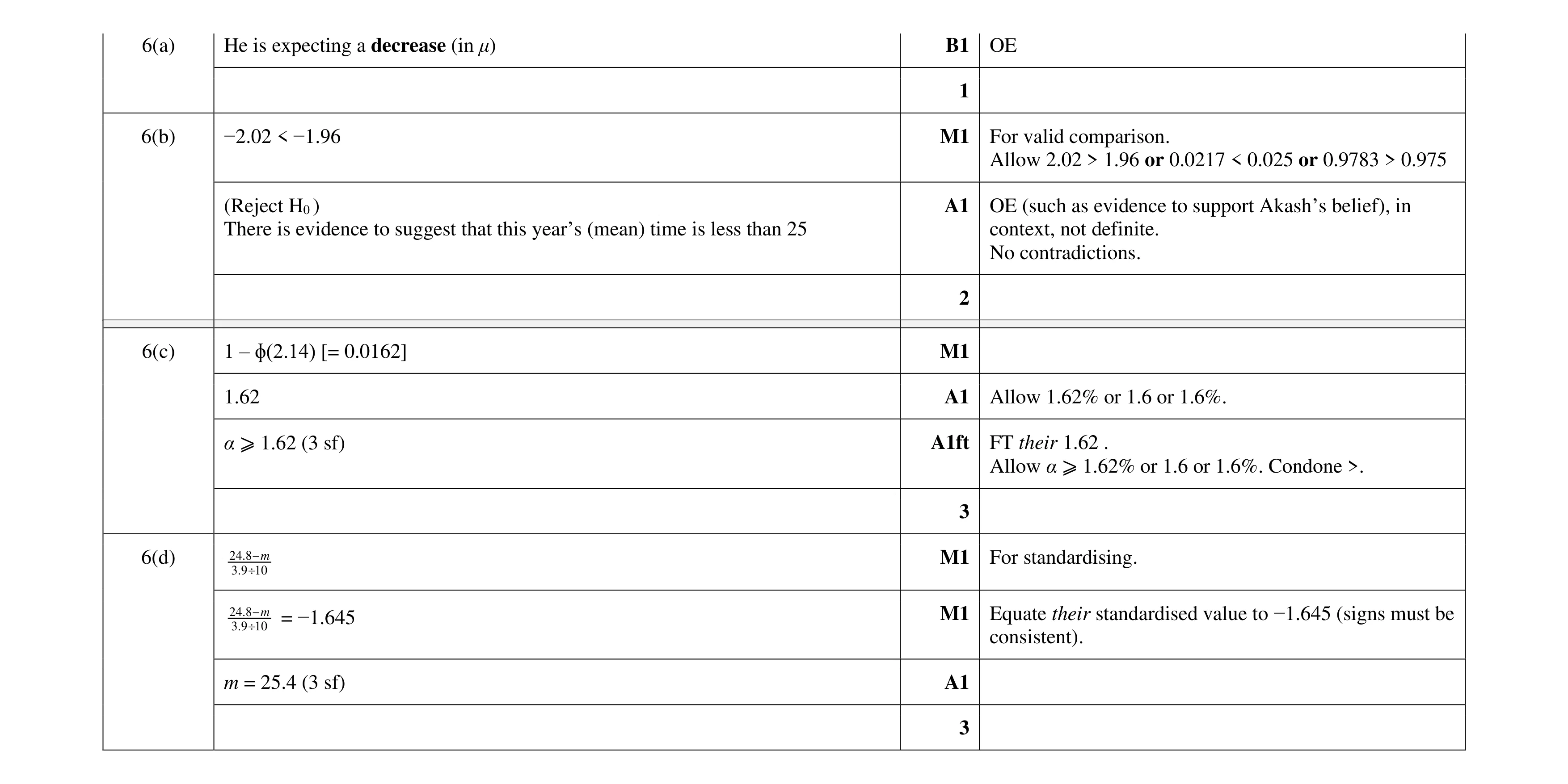 9
9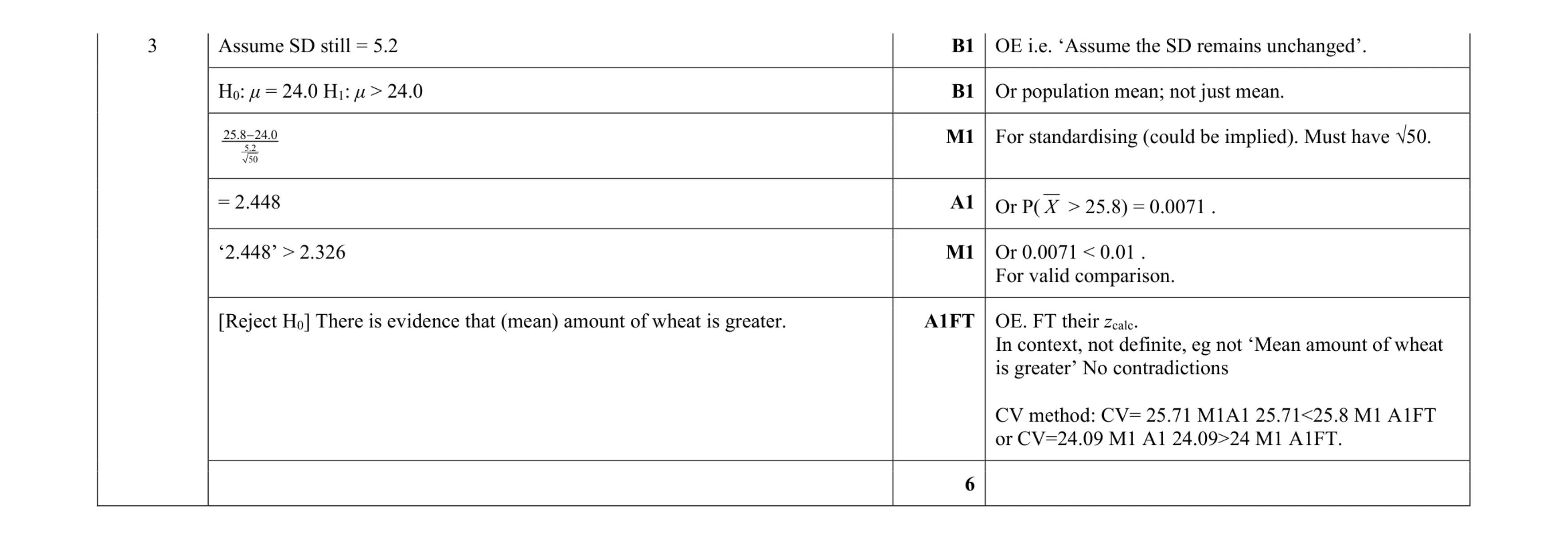 6
6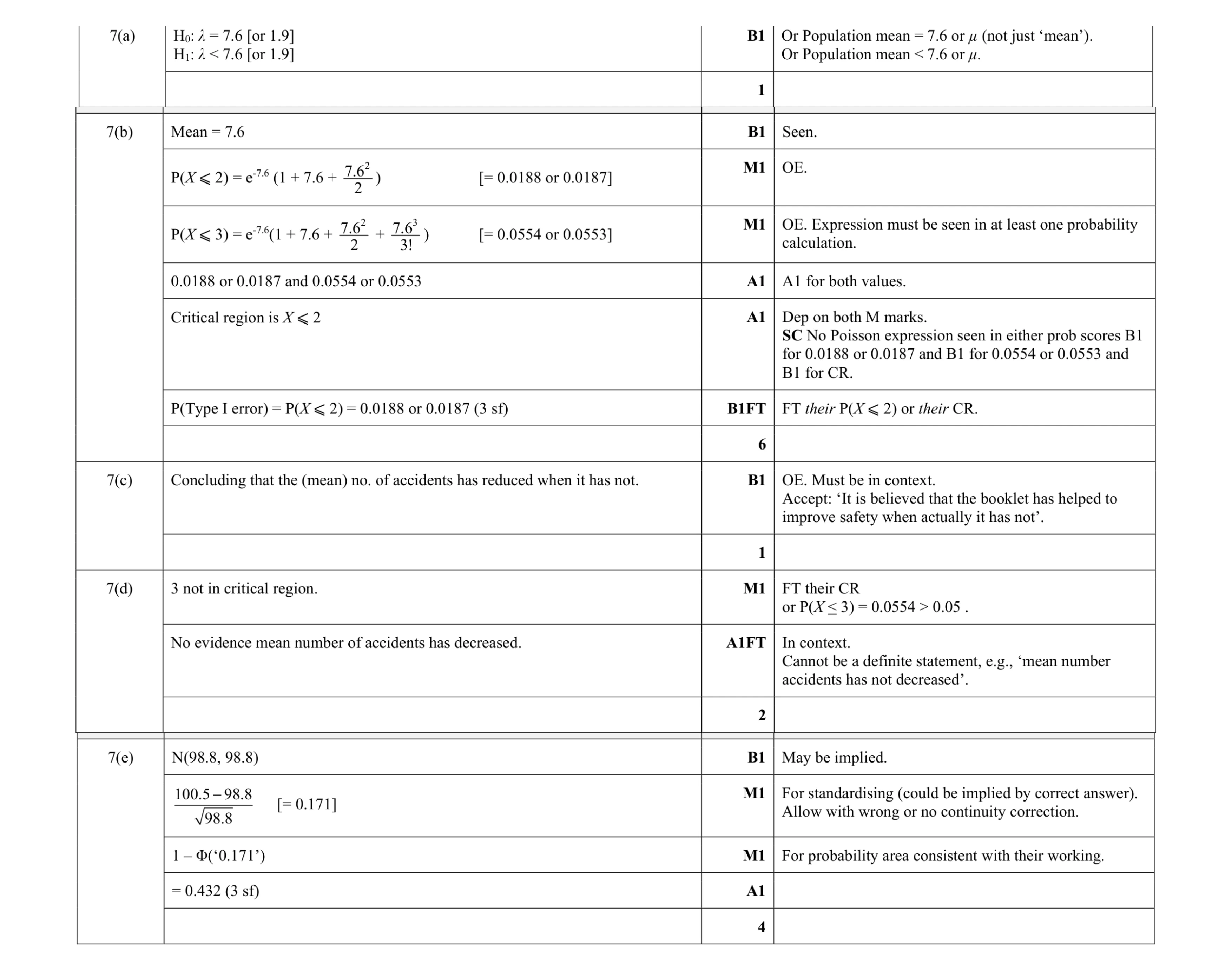 14
14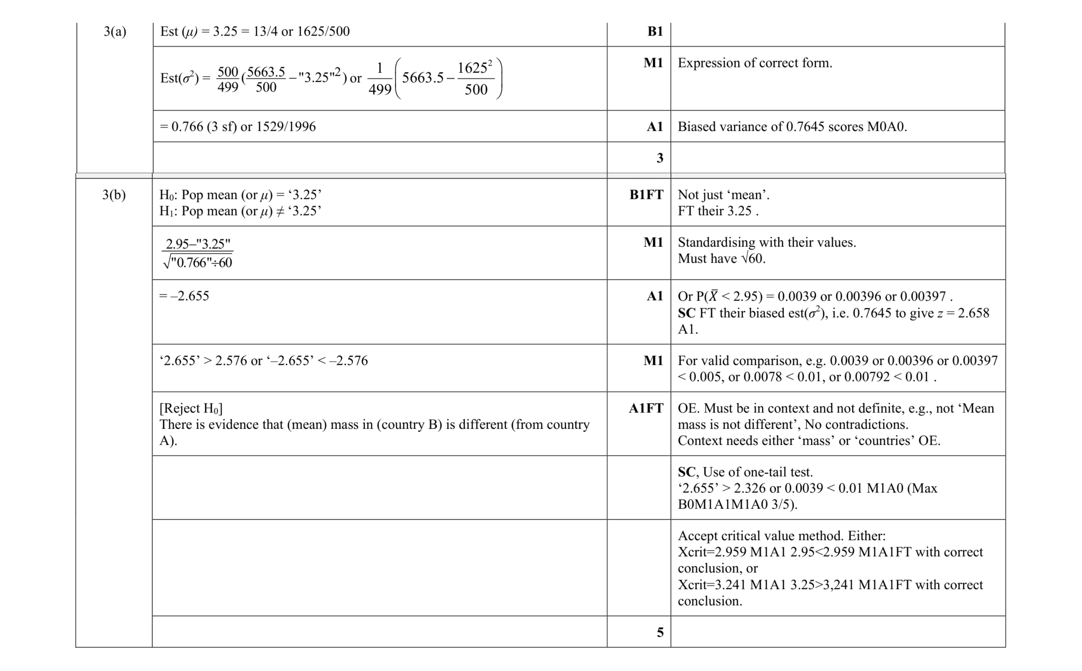 8
8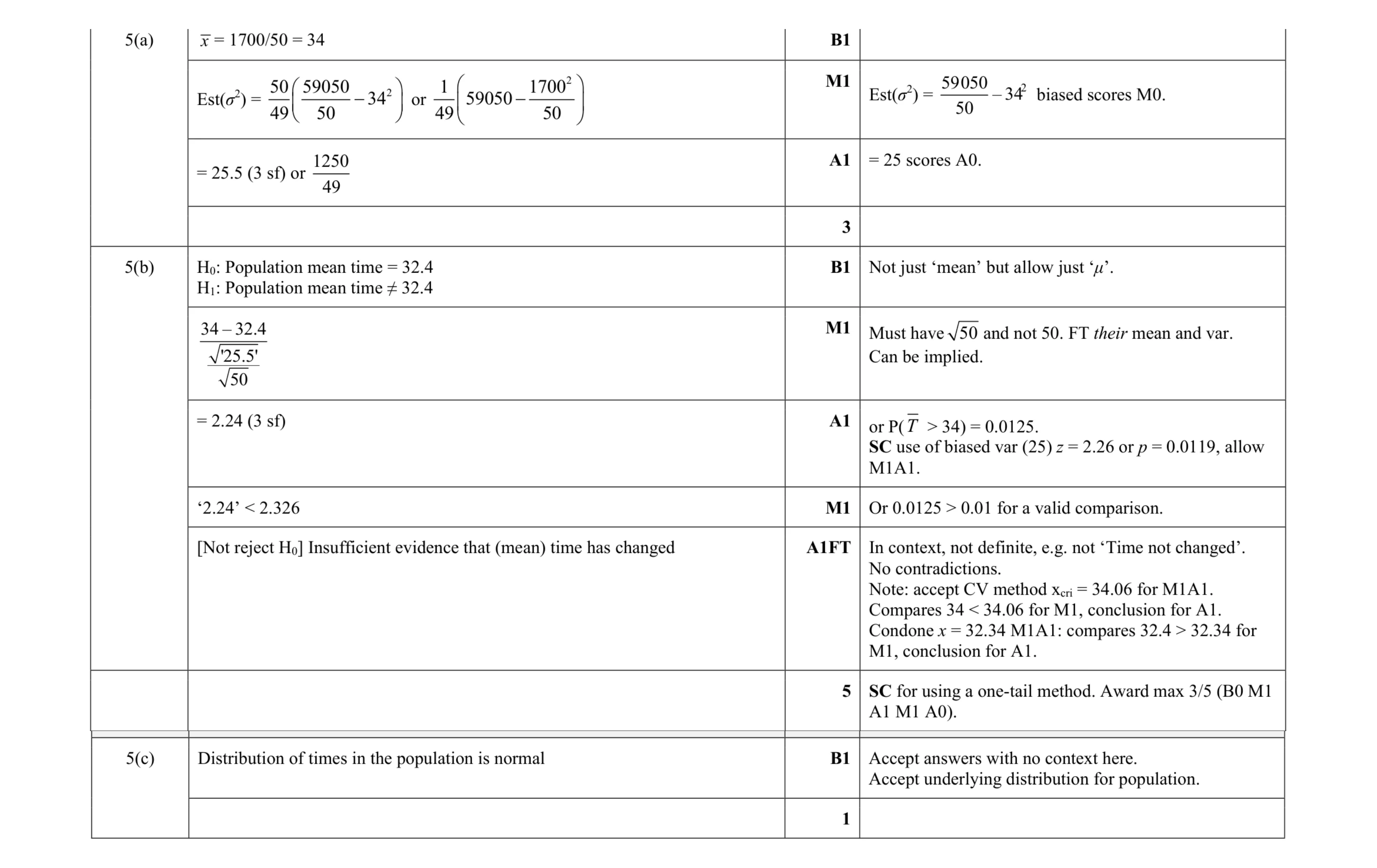 9
9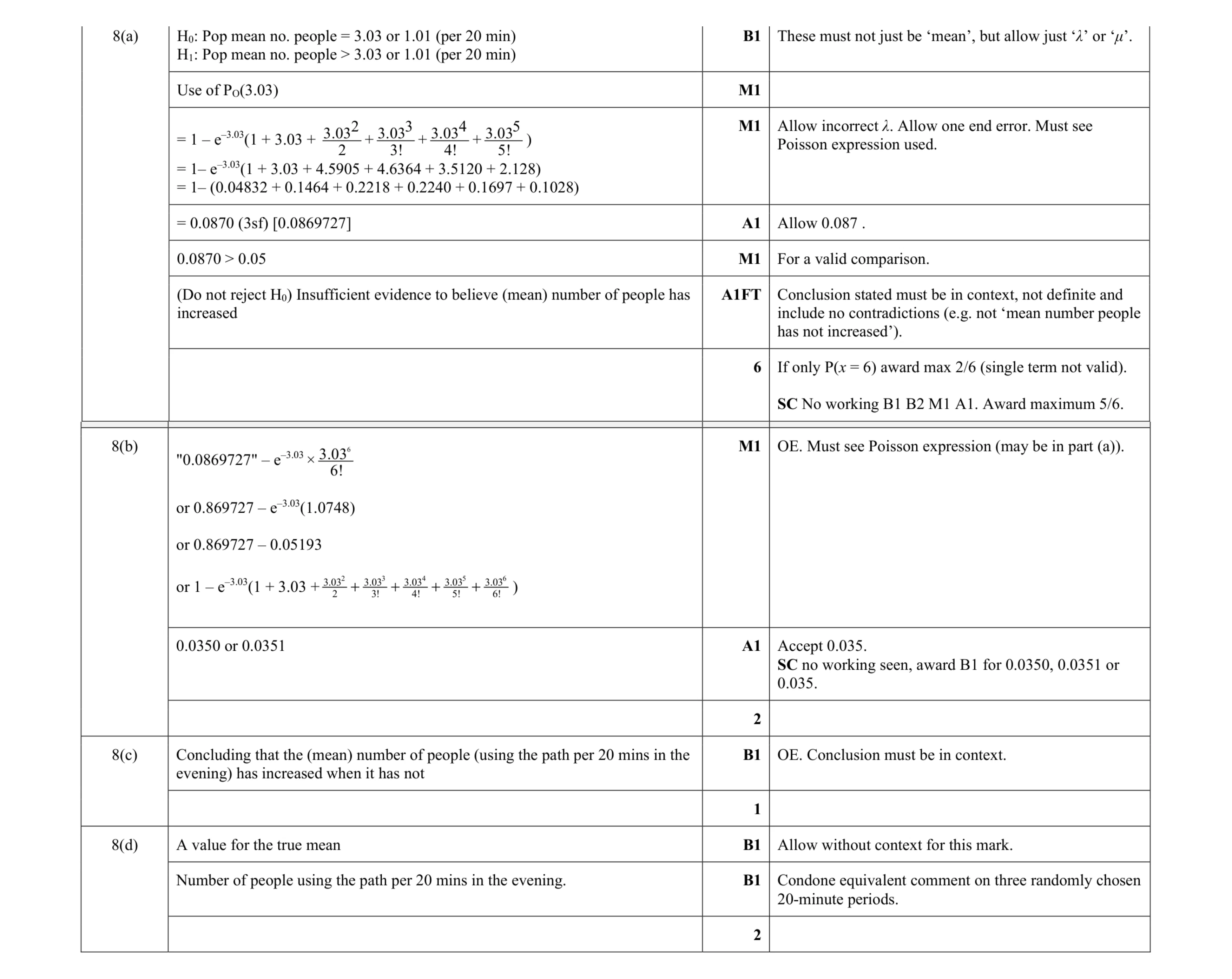 11
11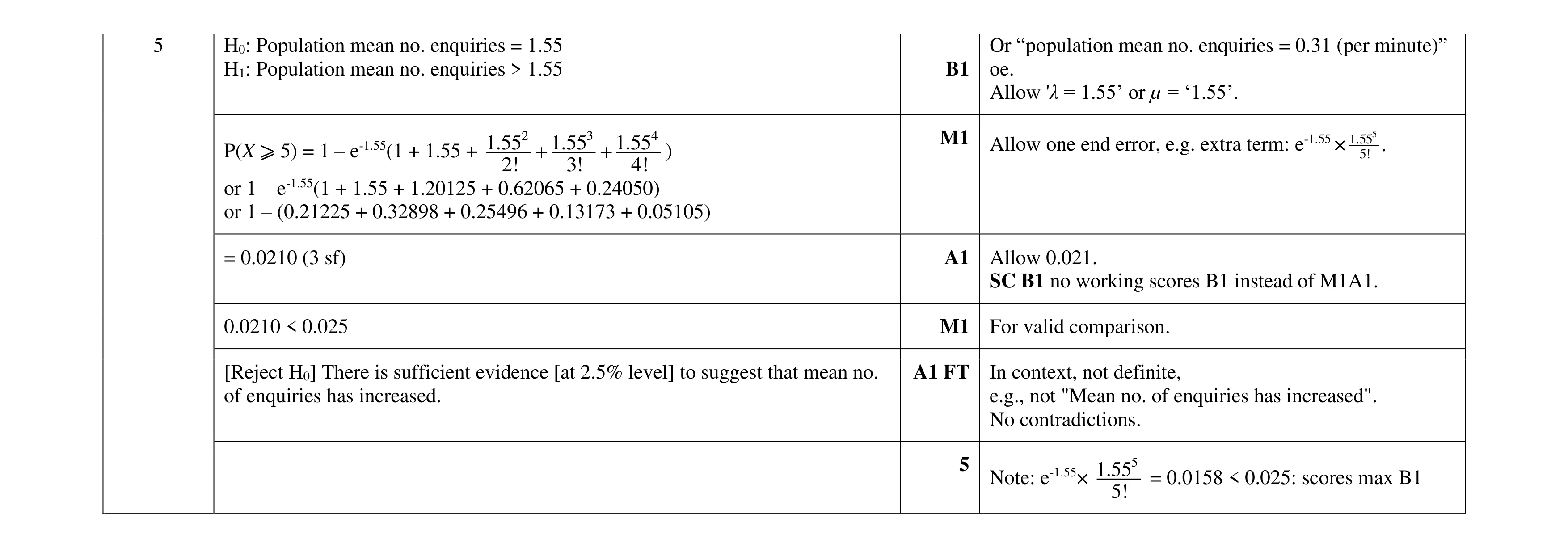 5
5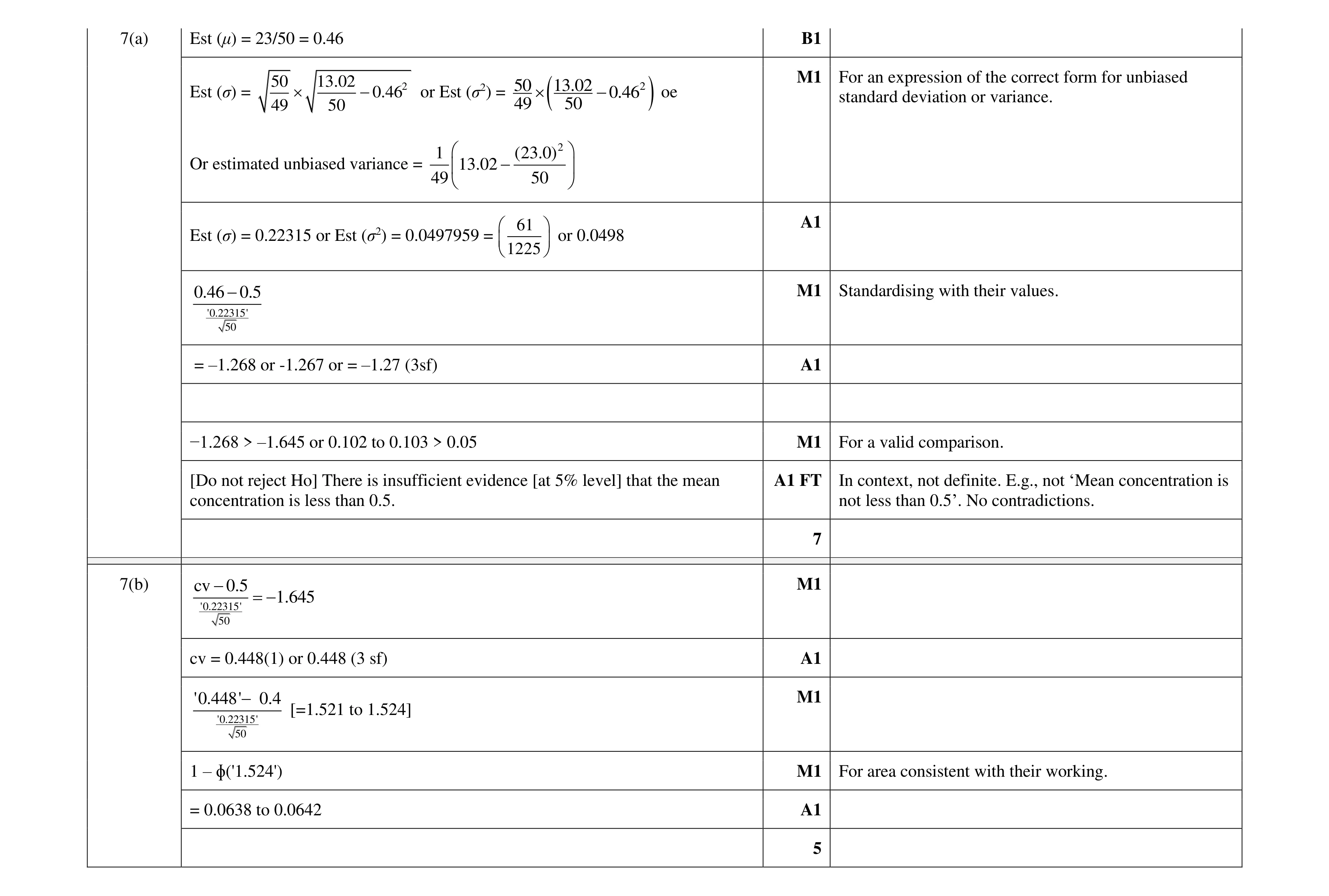 12
12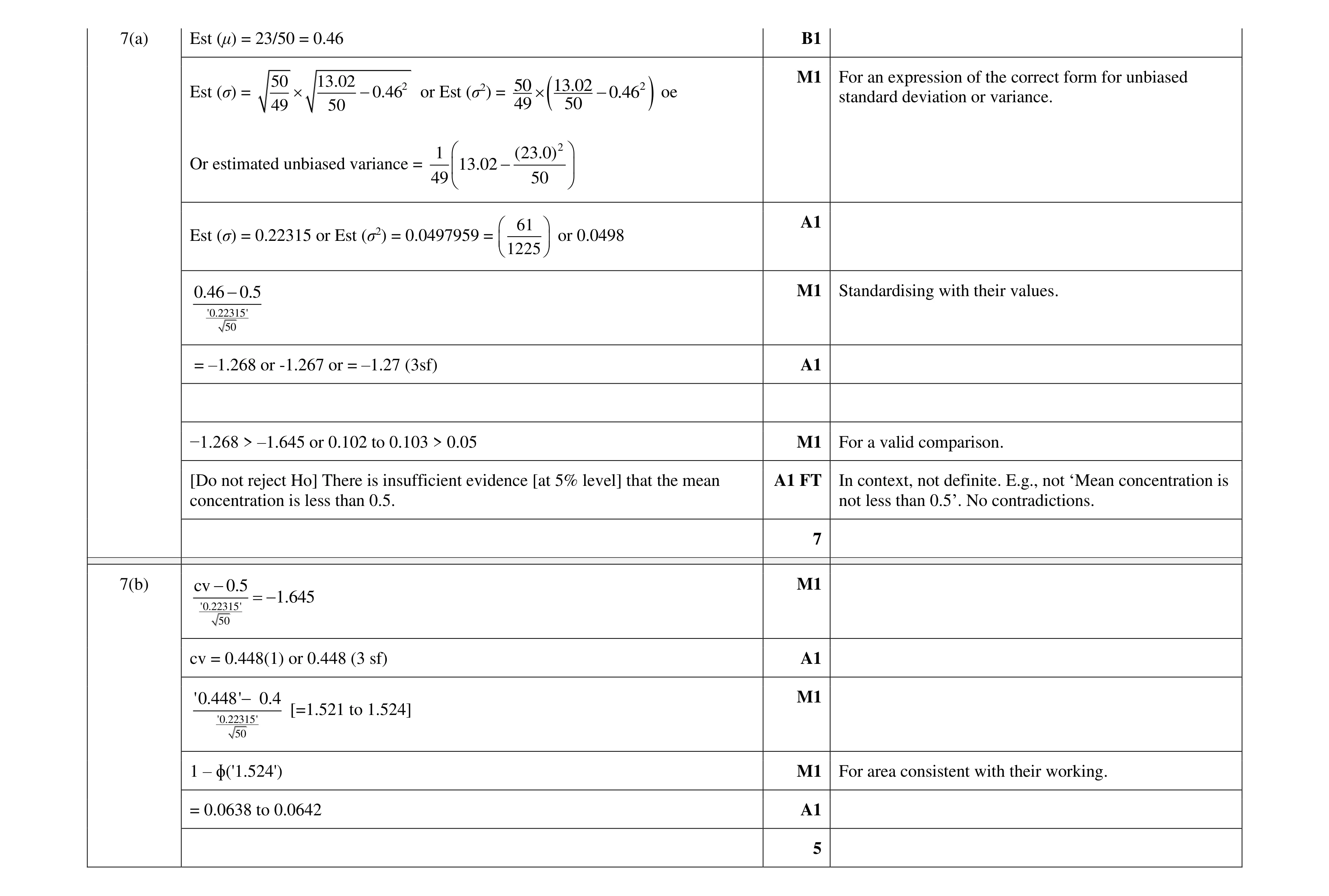 12
12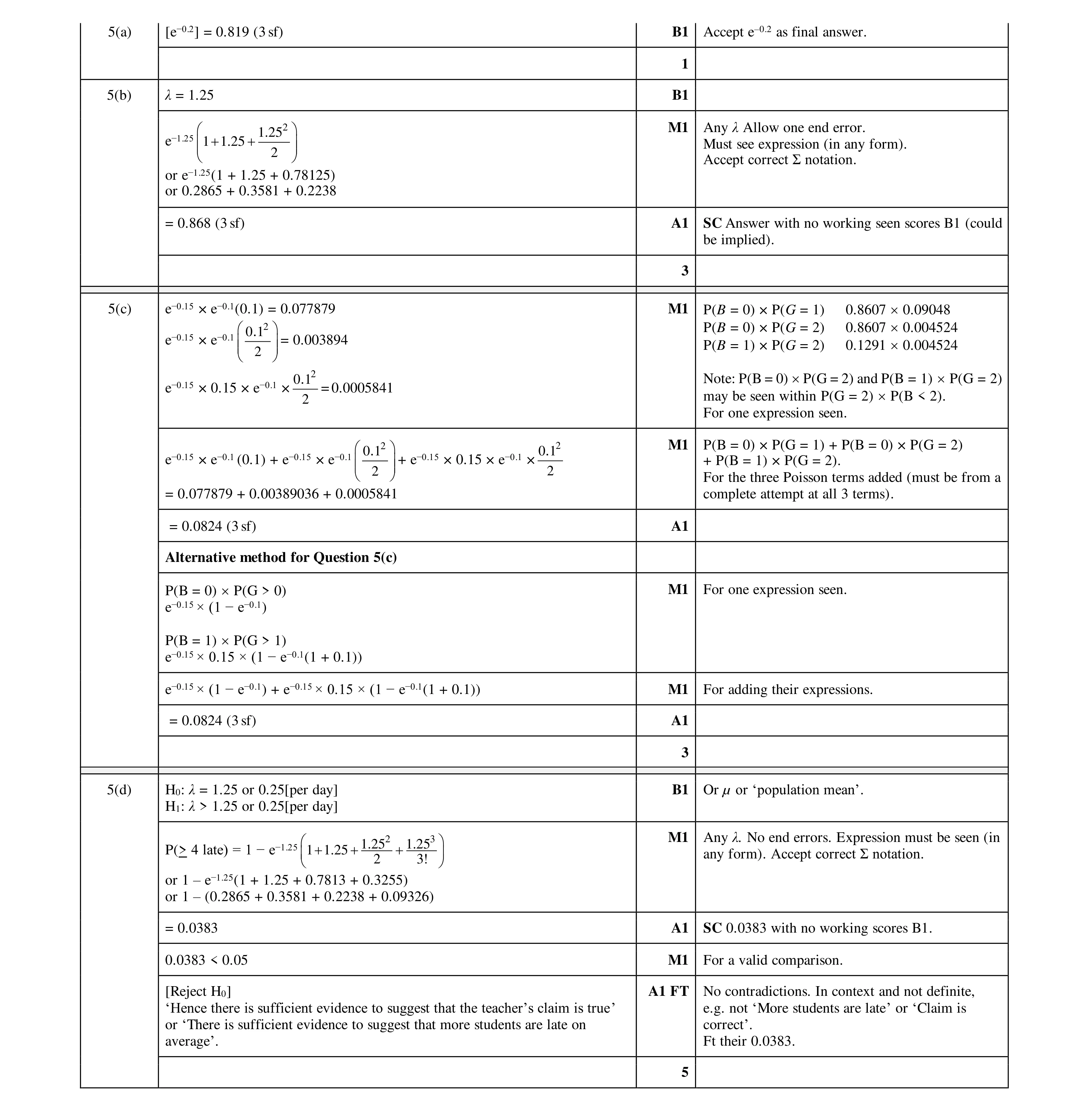 12
12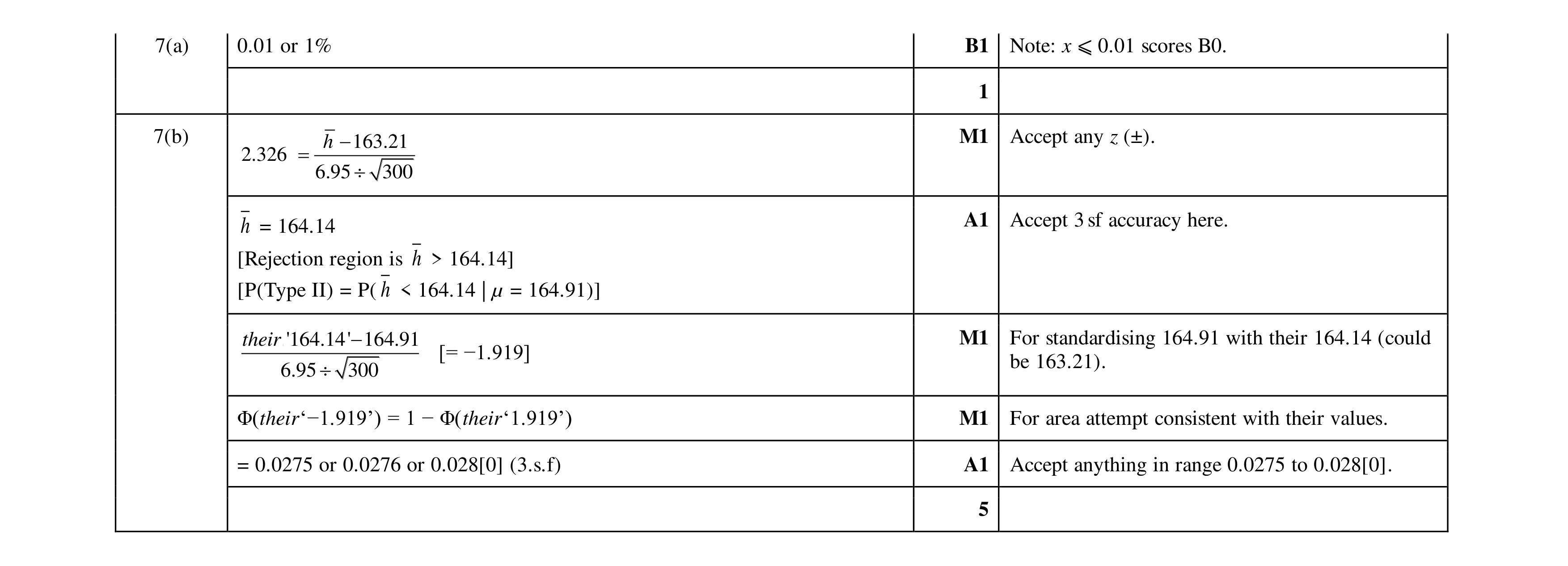 6
6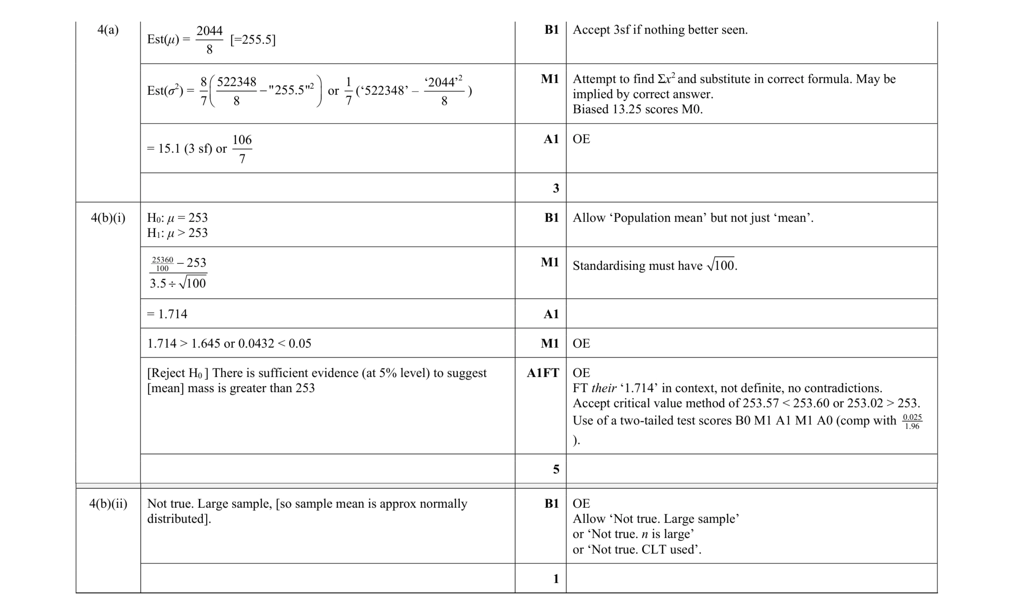 9
9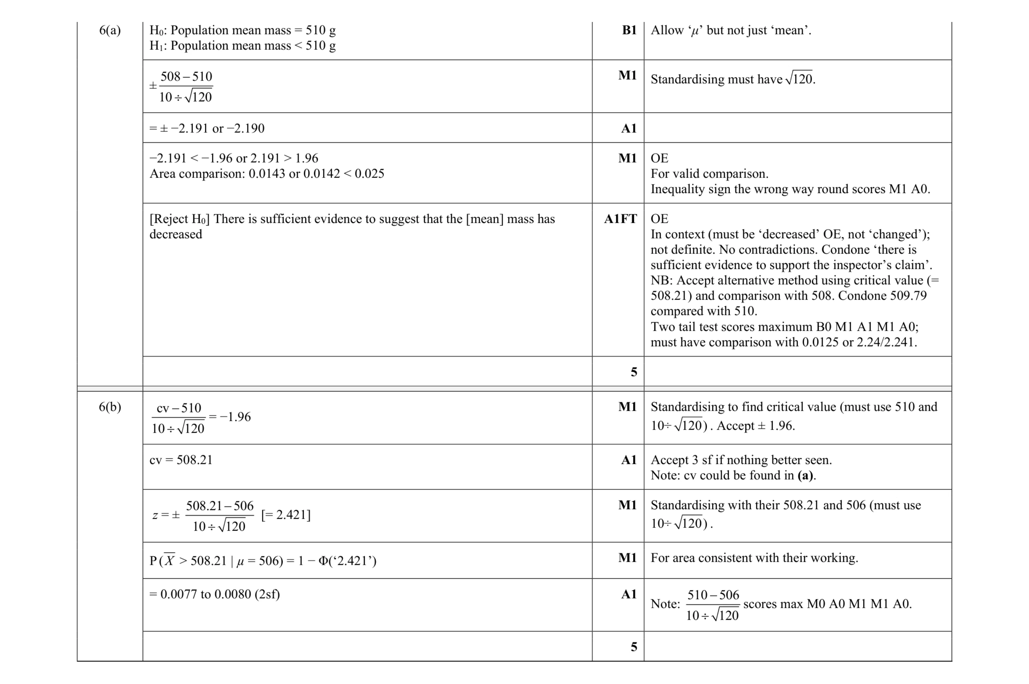 10
10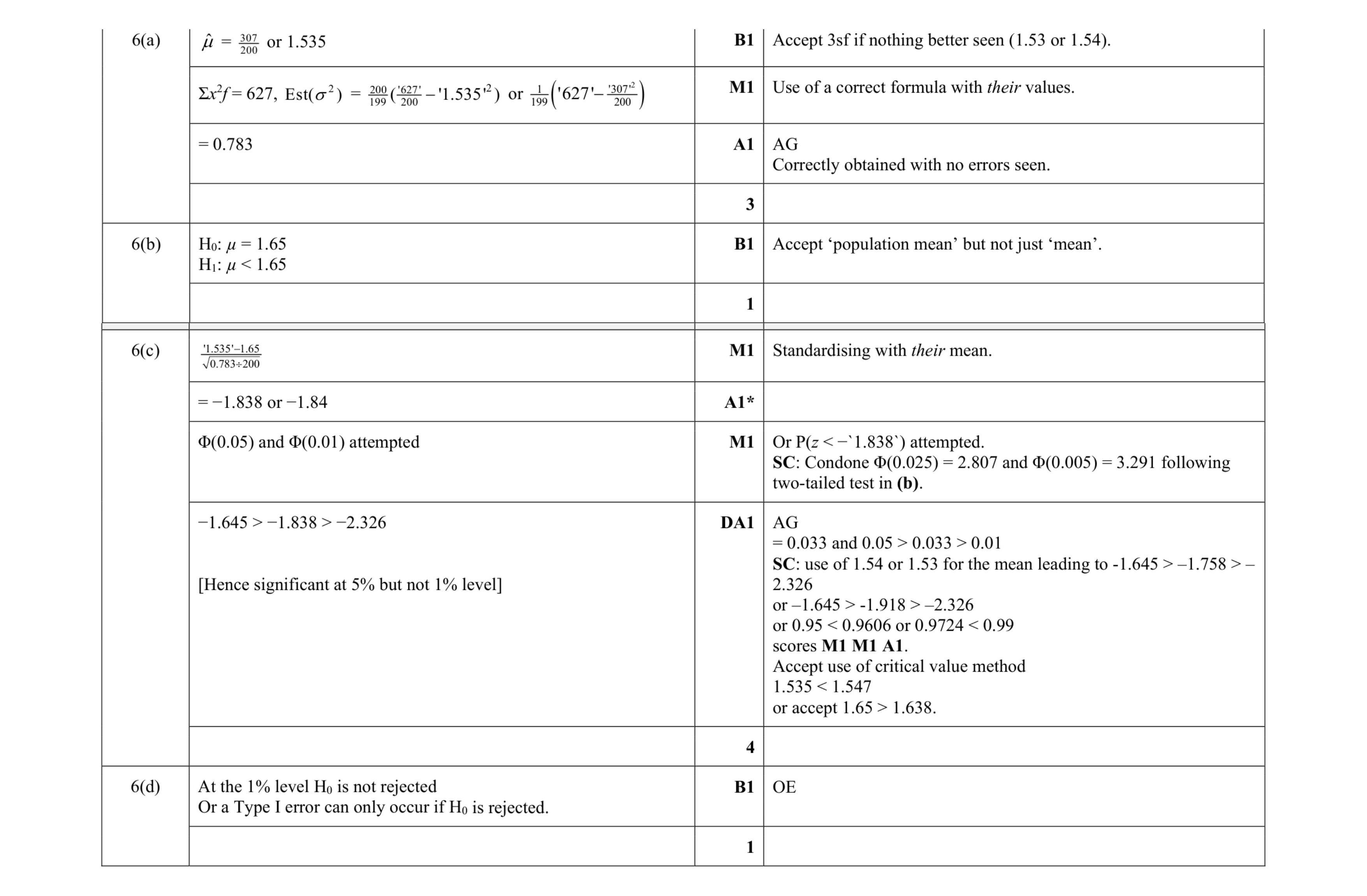 9
9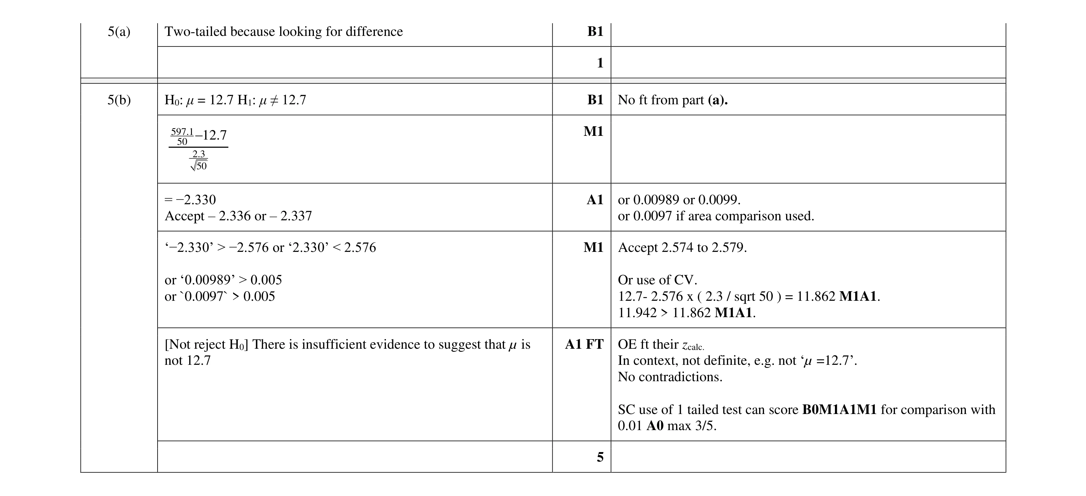 6
6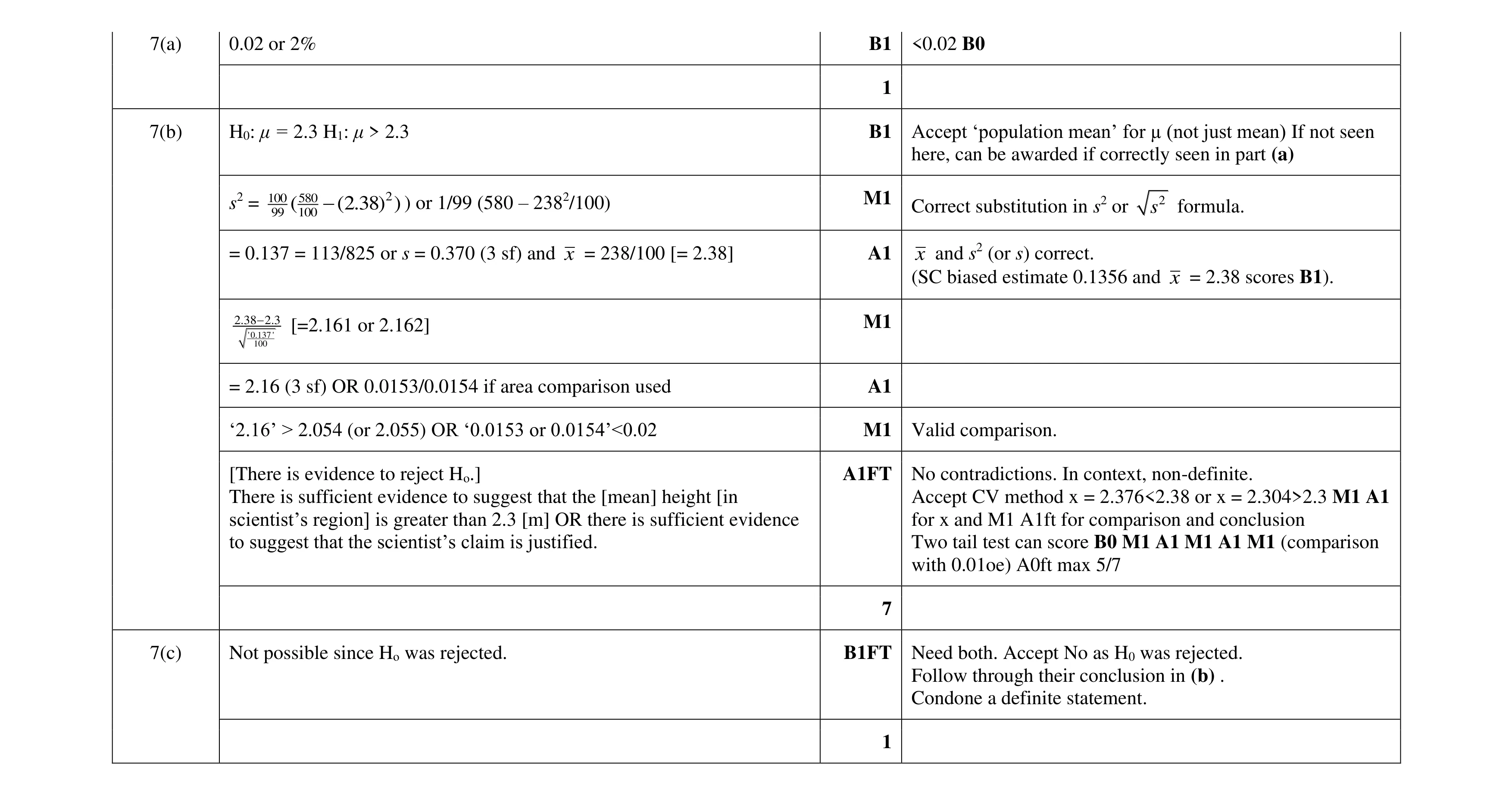 9
9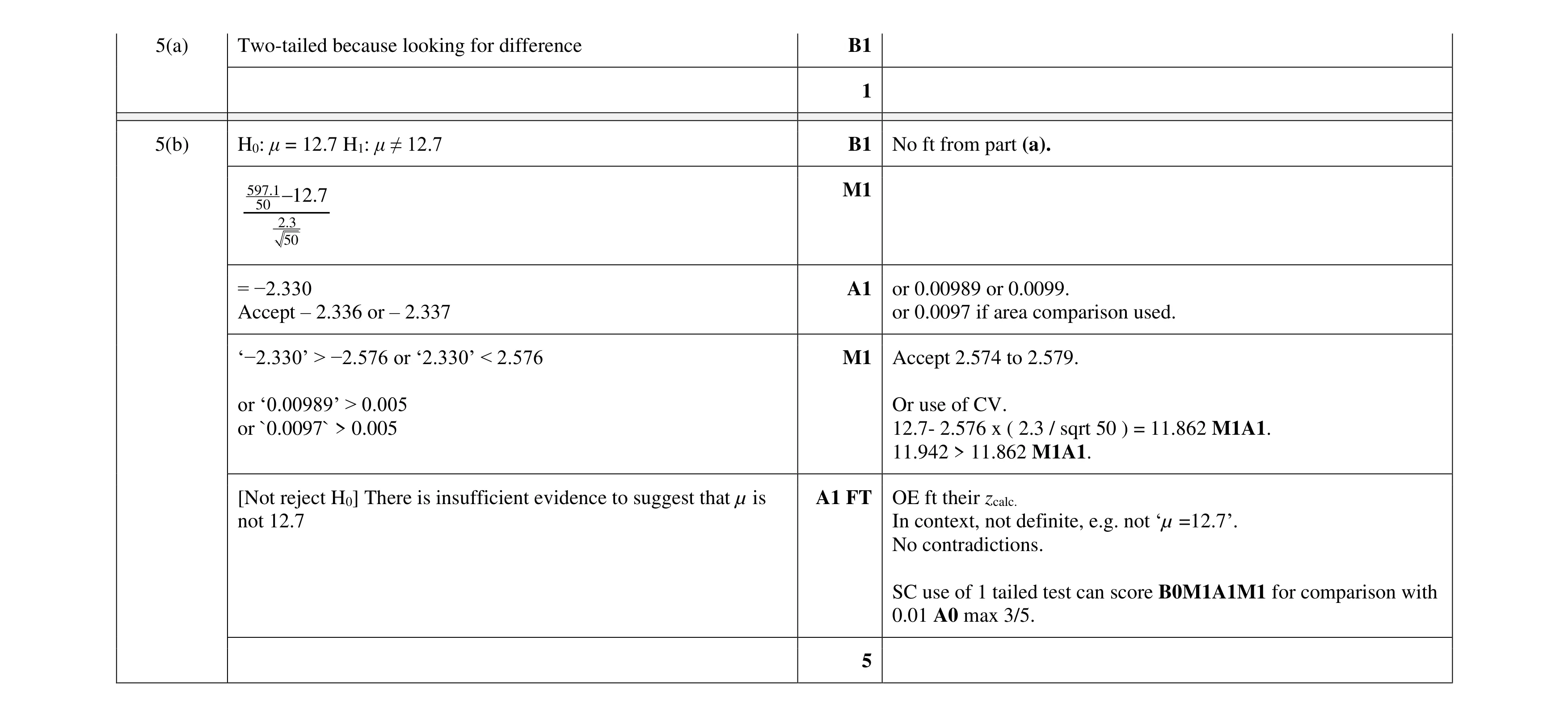 6
6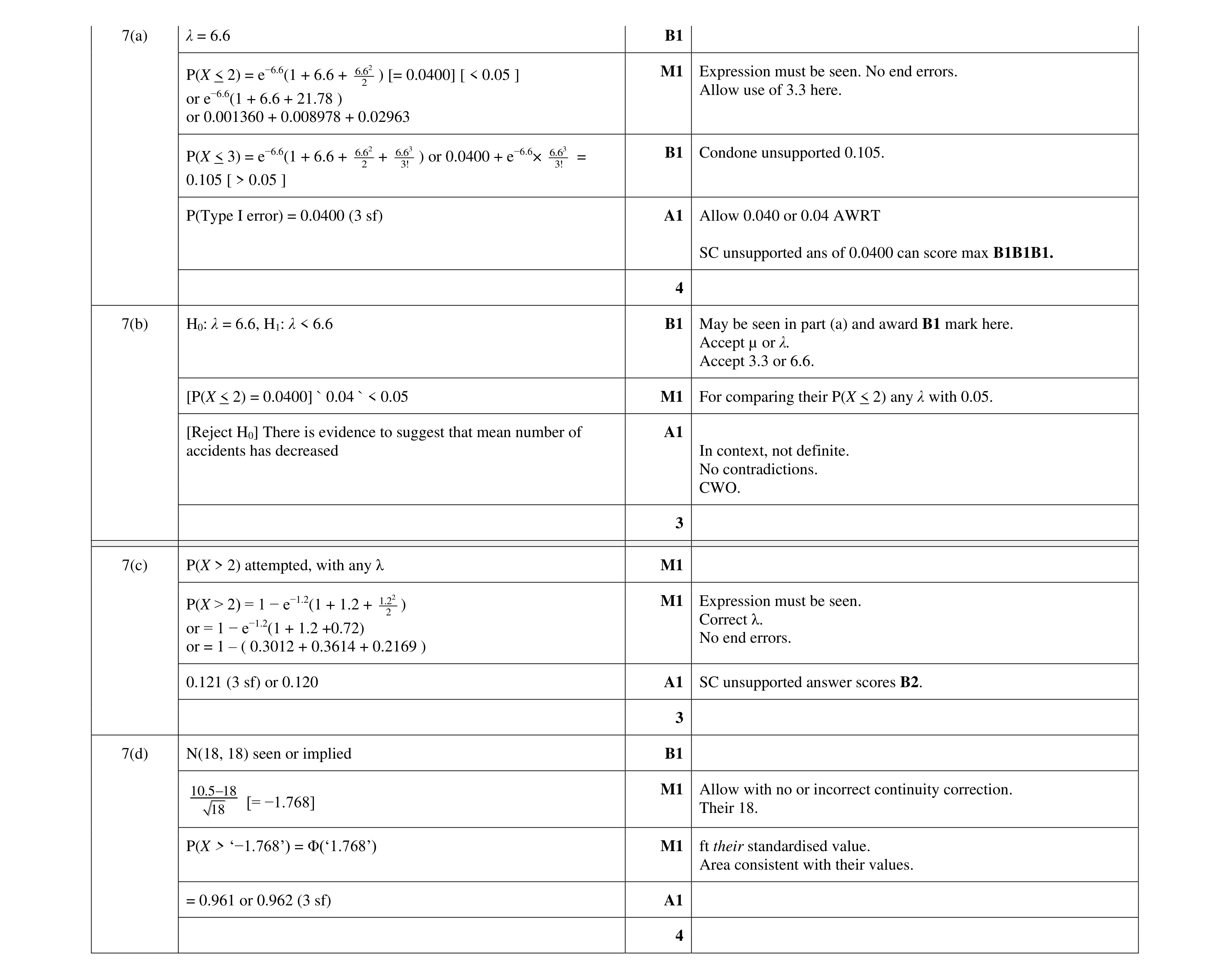 14
14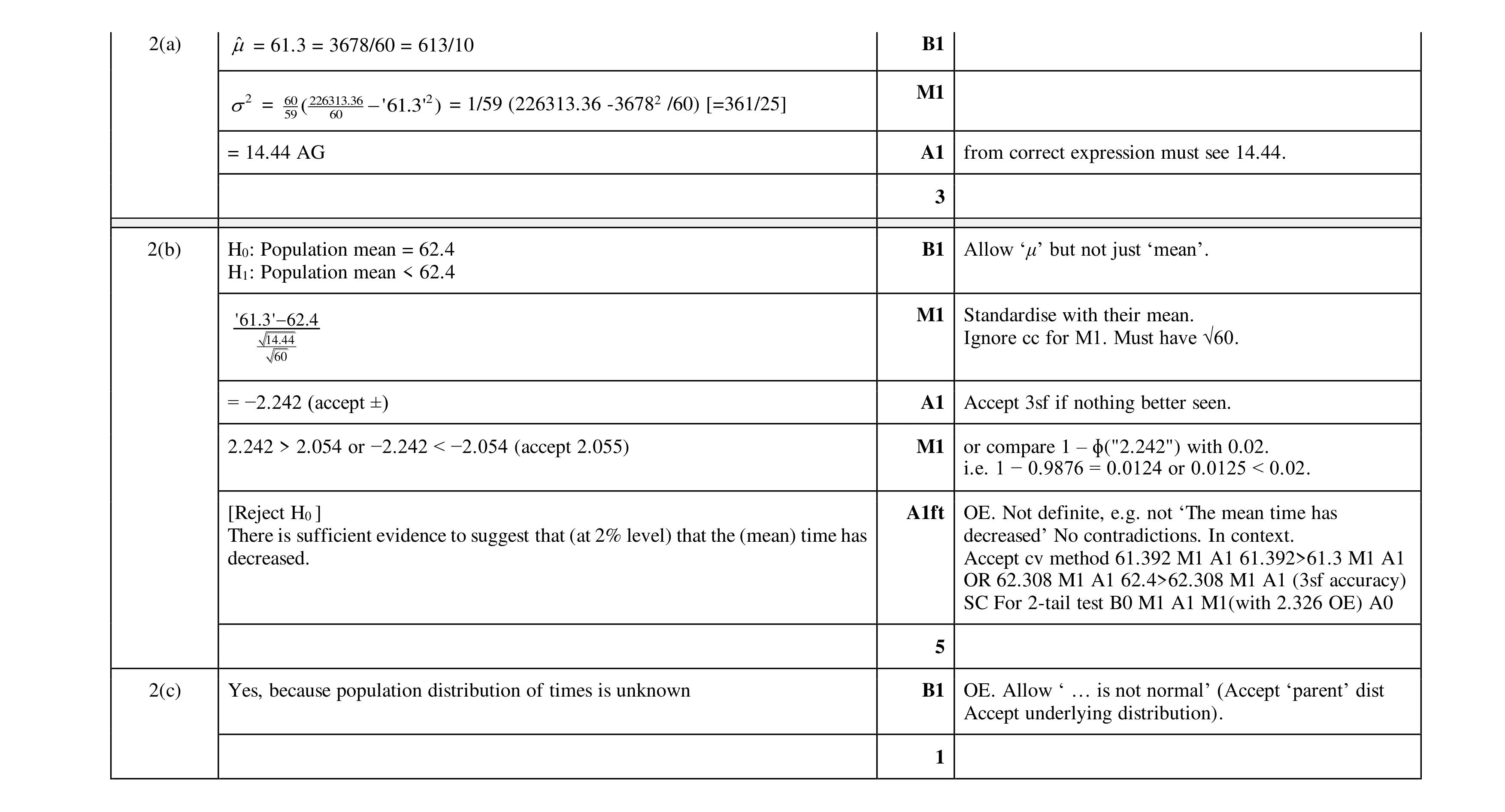 9
9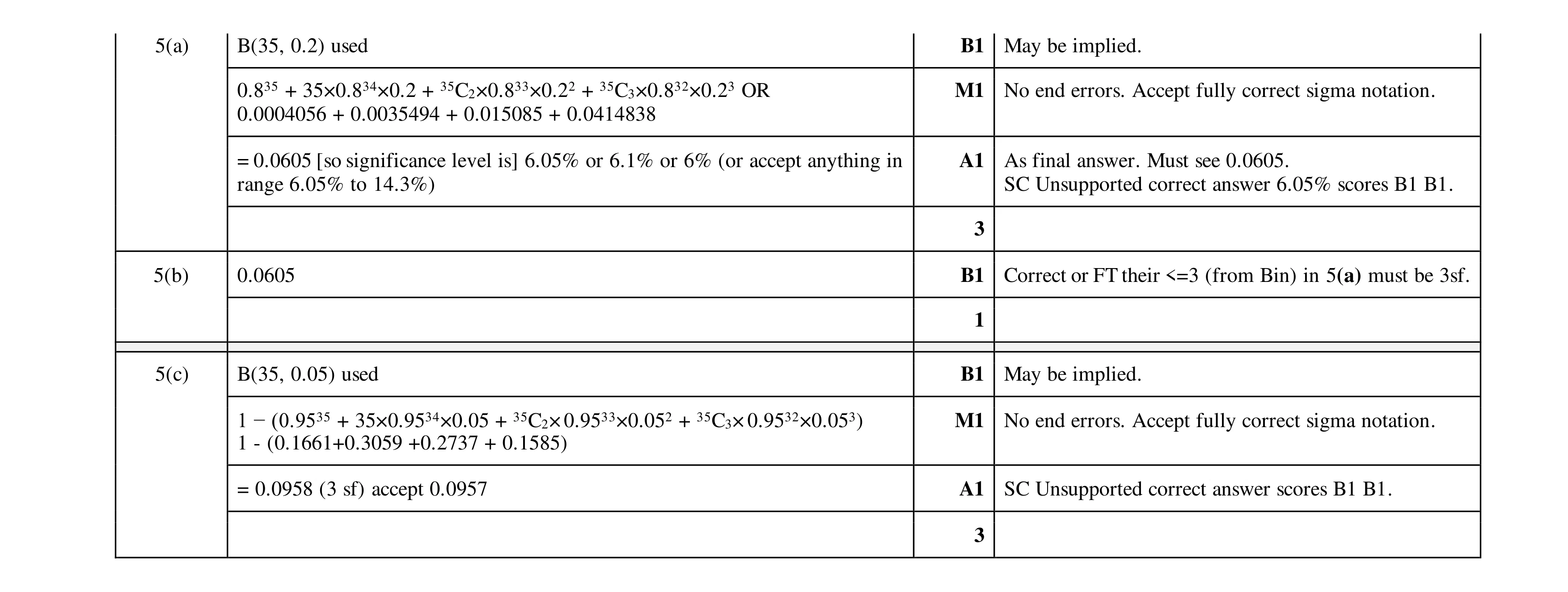 7
7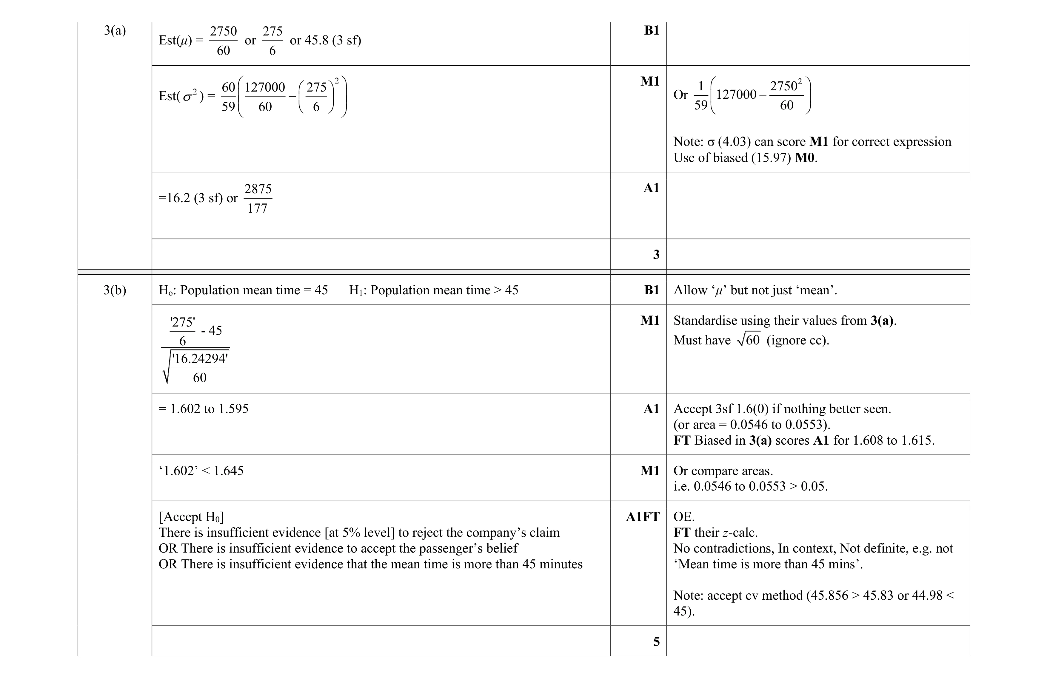 8
8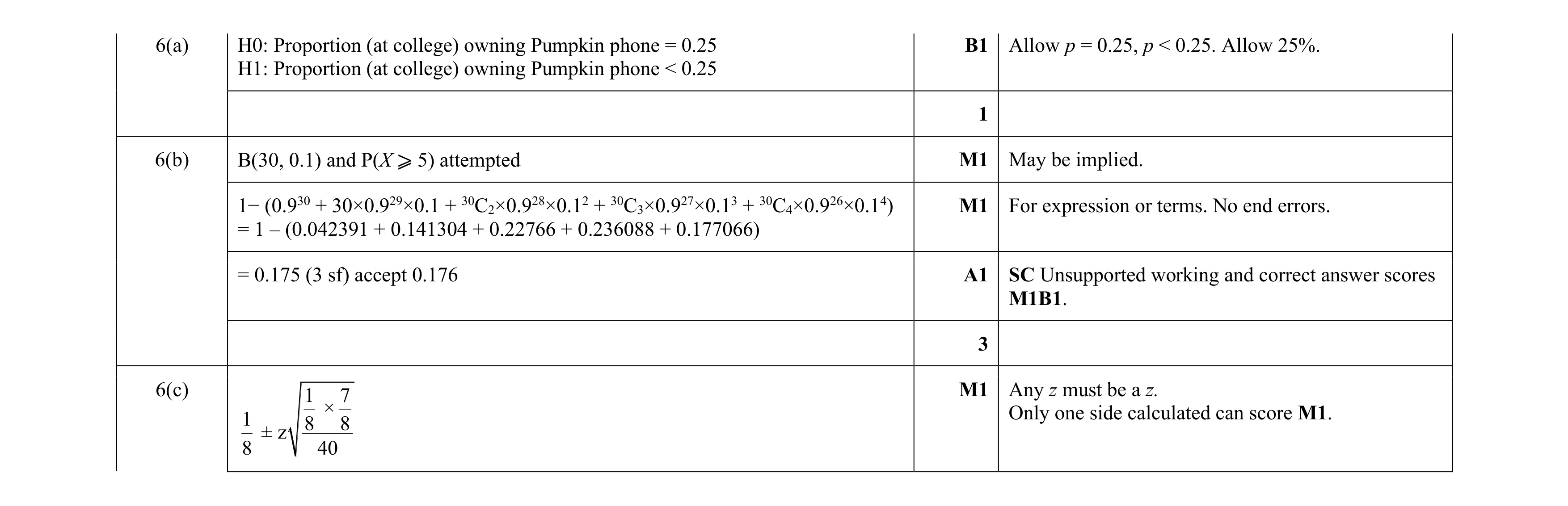 7
7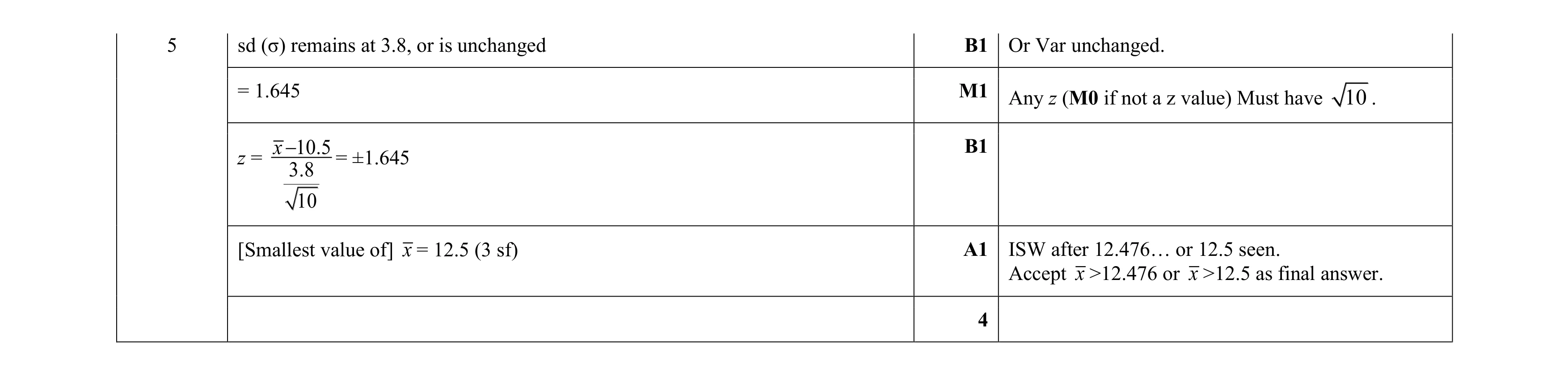 4
4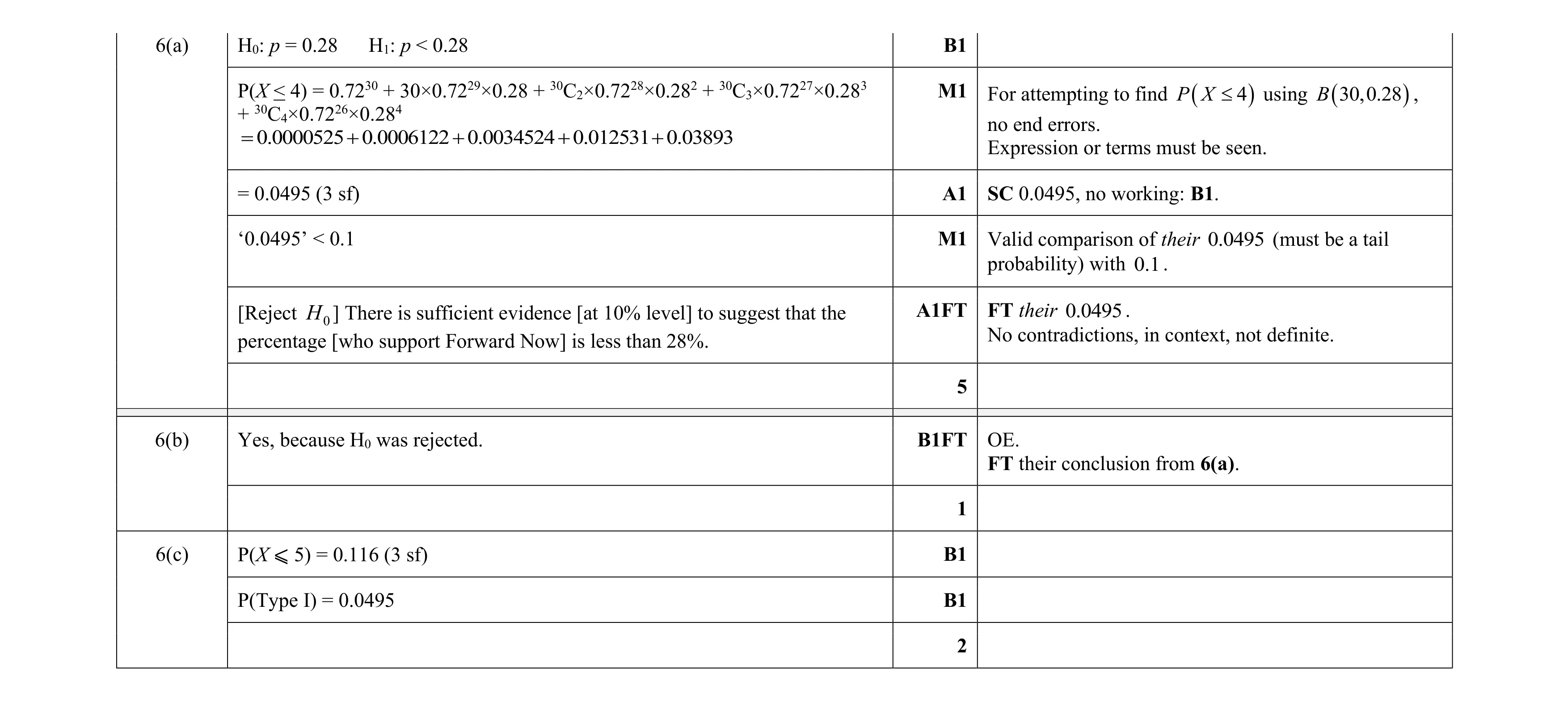 8
8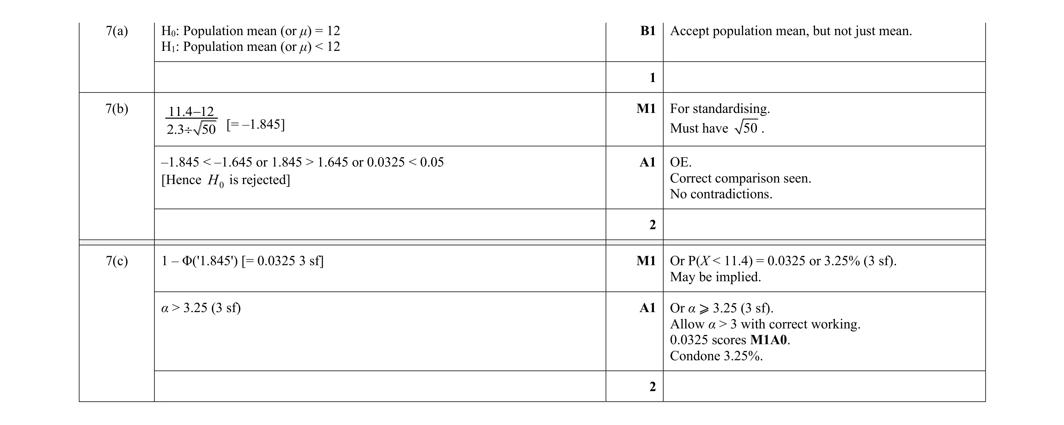 5
5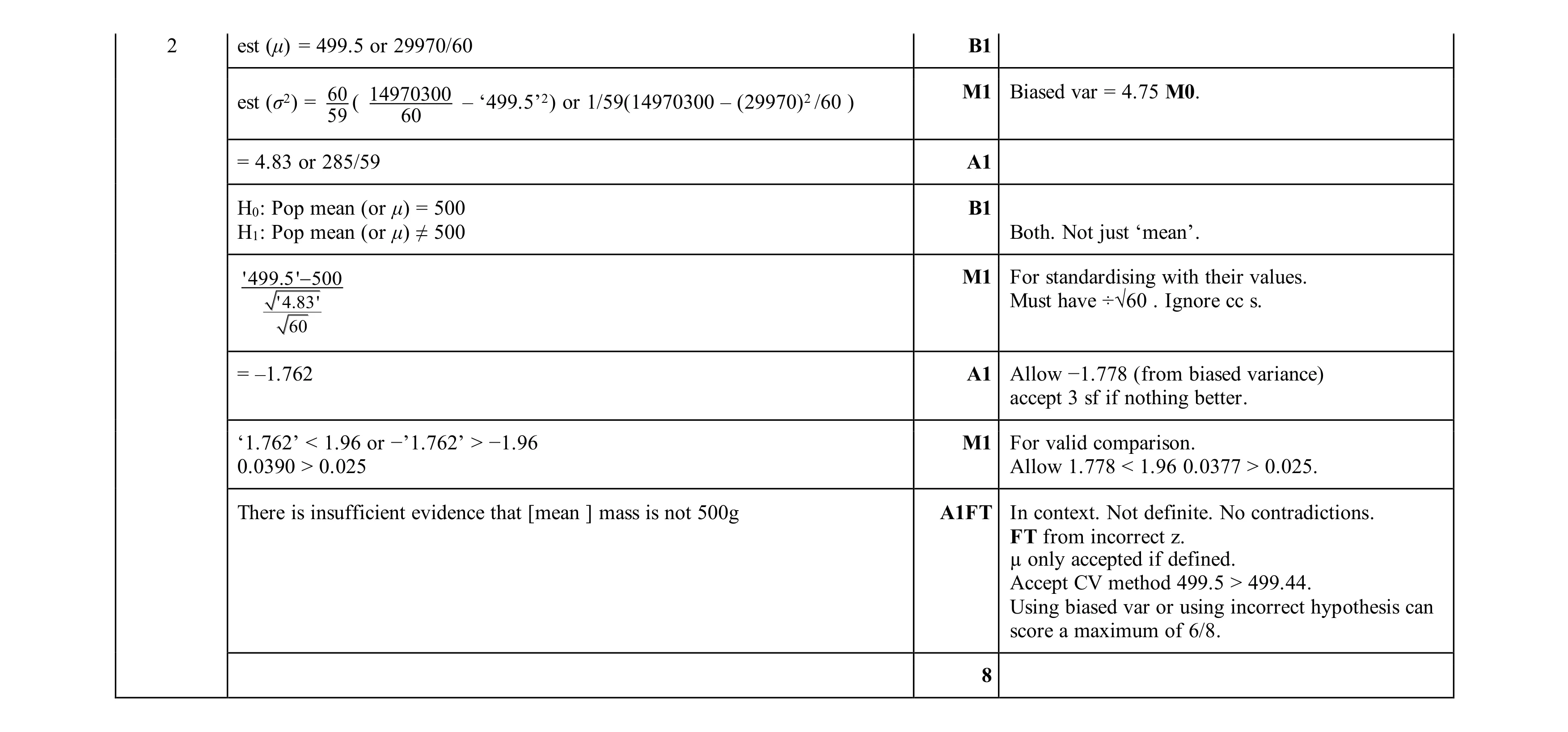 8
8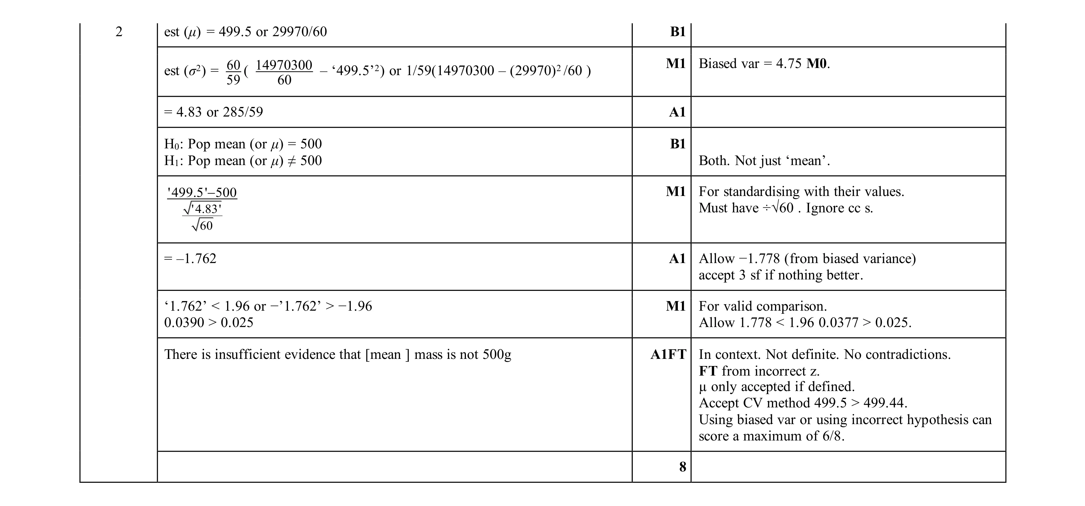 8
8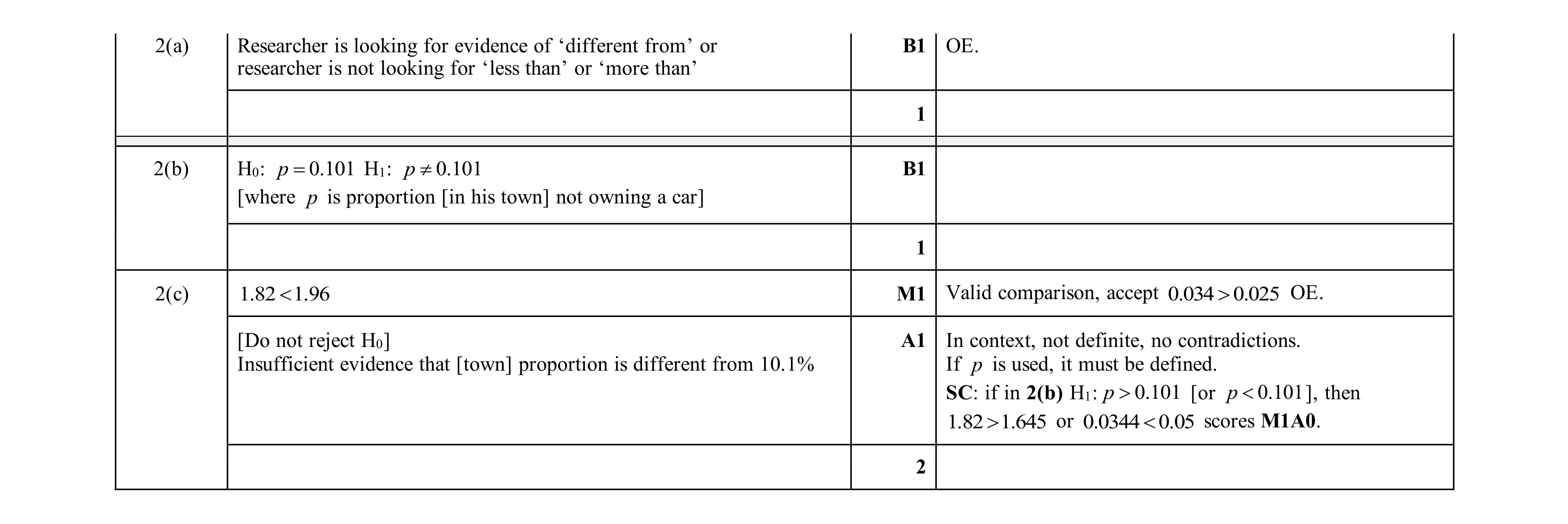 4
4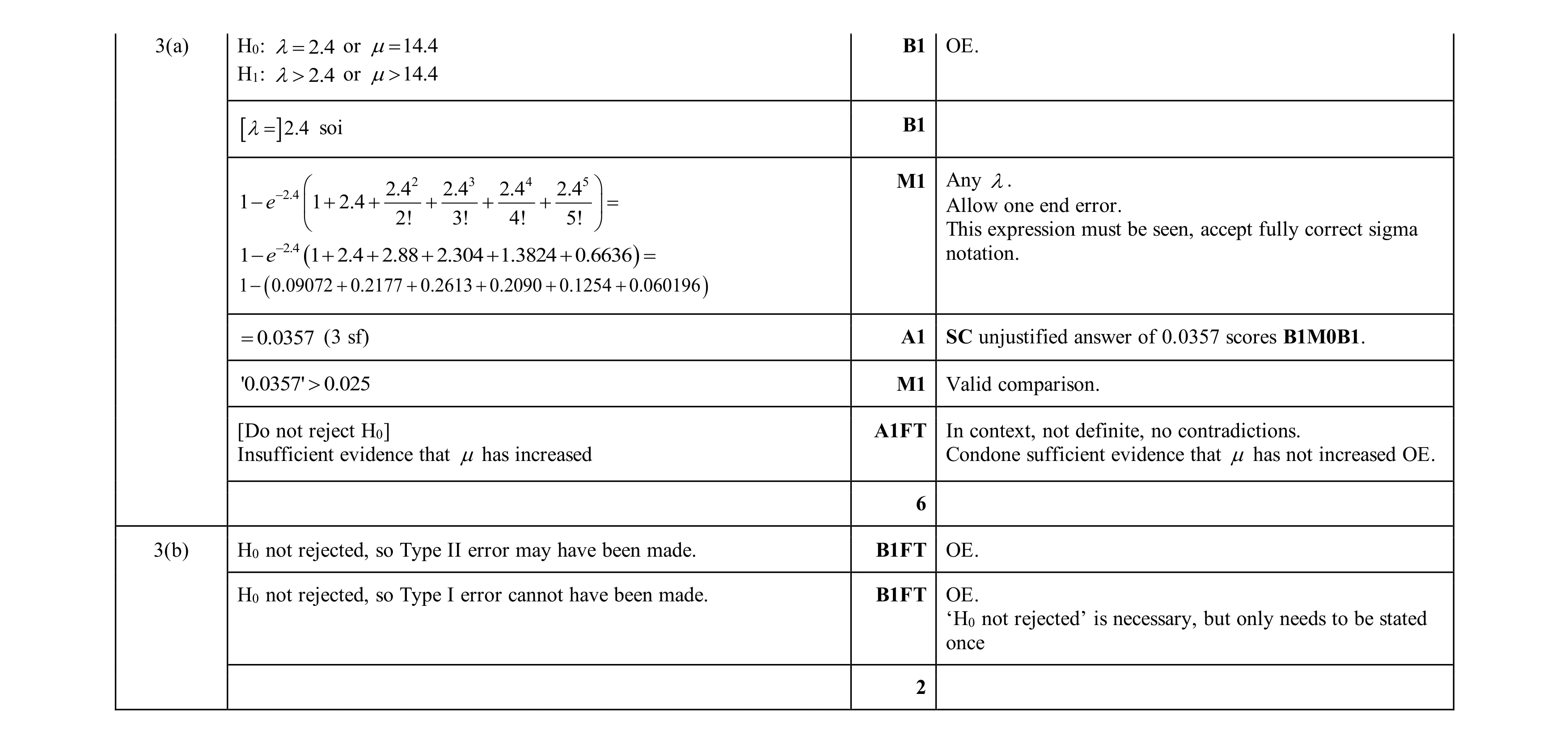 8
8