Questions as text
Q1 · The heights, x cm, of some plants are shown in the table 0607/41 May/June 2017
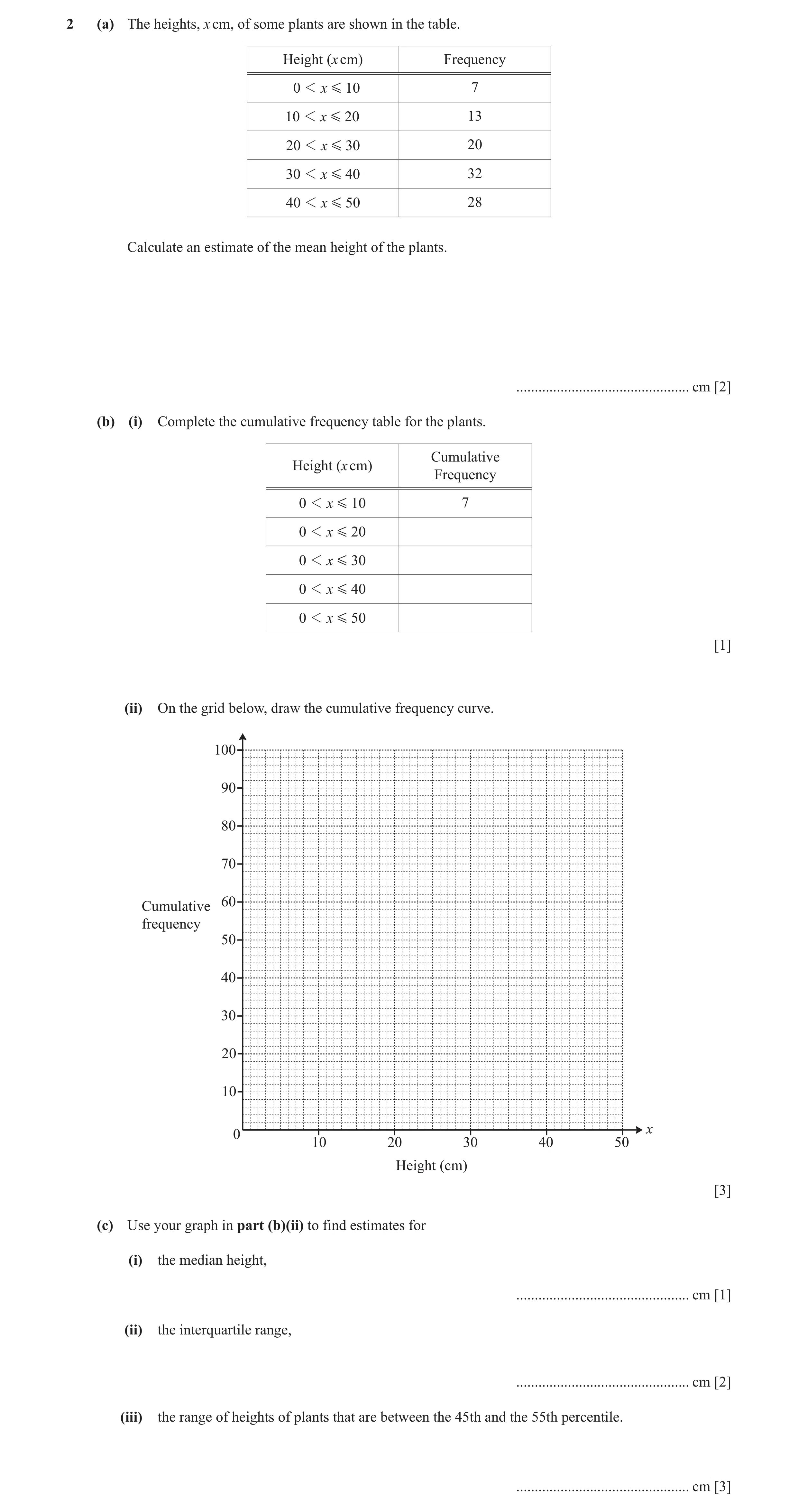
2 (a) The heights, x cm, of some plants are shown in the table. Height (x cm) Frequency 0 1 x G 10 7 10 1 x G 20 13 20 1 x G 30 20 30 1 x G 40 32 40 1 x G 50 28 Calculate an estimate of the mean height of the plants. … cm [2] (b) (i) Complete the cumulative frequency table for the plants. Cumulative Height (x cm) Frequency 0 1 x G 10 7 0 1 x G 20 0 1 x G 30 0 1 x G 40 0 1 x G 50 [1] (ii) On the grid below, draw the cumulative frequency curve. 100 90 80 70 60 Cumulative frequency 50 40 30 20 10 x 0 10 20 30 40 50 Height (cm) [3] (c) Use your graph in part (b)(ii) to find estimates for (i) the median height, … cm [1] (ii) the interquartile range, … cm [2] (iii) the range of heights of plants that are between the 45th and the 55th percentile. … cm [3]
12 marks
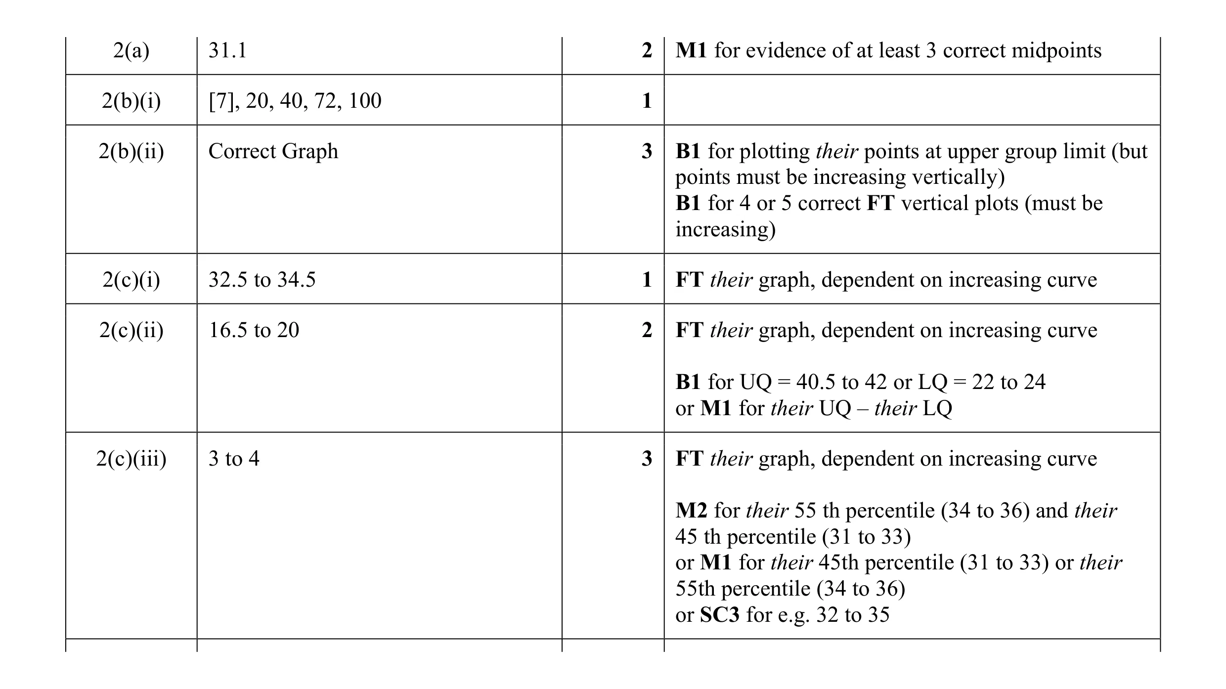
Mark scheme: 2(a) 31.1 2 M1 for evidence of at least 3 correct midpoints 2(b)(i) [7], 20, 40, 72, 100 1 2(b)(ii) Correct Graph 3 B1 for plotting their points at upper group limit (but points must be increasing vertically) B1 for 4 or 5 correct FT vertical plots (must be increasing) 2(c)(i) 32.5 to 34.5 1 FT their graph, dependent on increasing curve 2(c)(ii) 16.5 to 20 2 FT their graph, dependent on increasing curve B1 for UQ = 40.5 to 42 or LQ = 22 to 24 or M1 for their UQ – their LQ 2(c)(iii) 3 to 4 3 FT their graph, dependent on increasing curve M2 for their 55 th percentile (34 to 36) and their 45 th percentile (31 to 33) or M1 for their 45th percentile (31 to 33) or their 55th percentile (34 to 36) or SC3 for e.g. 32 to 35
This question in 0607/41 May/June 2017
Q2 · The list shows the temperature, in degrees Celsius, at noon in Paris on each of 14 days 0607/41 May/June 2018
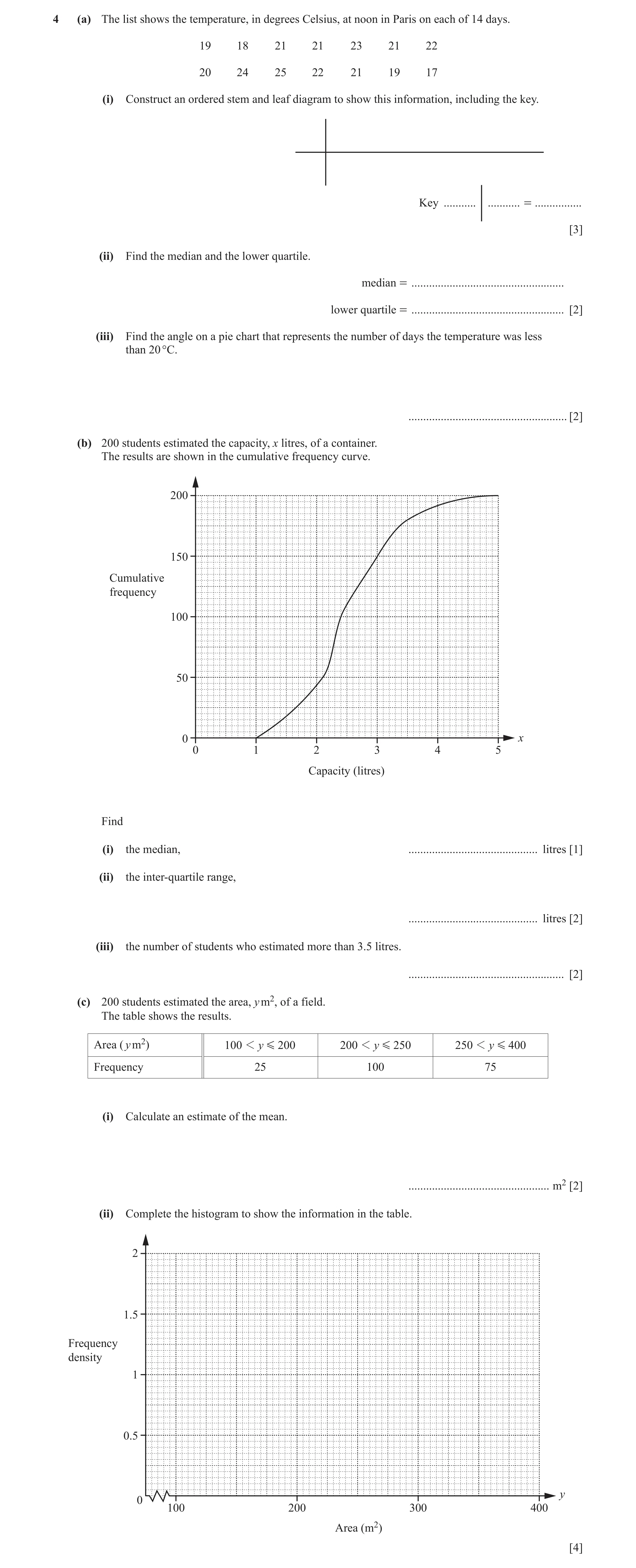
4 (a) The list shows the temperature, in degrees Celsius, at noon in Paris on each of 14 days. 19 18 21 21 23 21 22 20 24 25 22 21 19 17 (i) Construct an ordered stem and leaf diagram to show this information, including the key. Key … … = … [3] (ii) Find the median and the lower quartile. median = … lower quartile = … [2] (iii) Find the angle on a pie chart that represents the number of days the temperature was less than 20 °C. … [2] (b) 200 students estimated the capacity, x litres, of a container. The results are shown in the cumulative frequency curve. 200 150 Cumulative frequency 100 50 0 x 0 1 2 3 4 5 Capacity (litres) Find (i) the median, … litres [1] (ii) the inter-quartile range, … litres [2] (iii) the number of students who estimated more than 3.5 litres. … [2] (c) 200 students estimated the area, y m2, of a field. The table shows the results. Area (y m2) 100 1 y G 200 200 1 y G 250 250 1 y G 400 Frequency 25 100 75 (i) Calculate an estimate of the mean. … m2 [2] (ii) Complete the histogram to show the information in the table. 2 1.5 Frequency density 1 0.5 y 0 100 200 300 400 Area (m2) [4]
18 marks
Mark scheme: 4(a)(i) 1 7 8 9 9 3 B1for each row 2 0 1 1 1 1 2 2 3 4 5 B1 for key e.g. 2|3 = 23 4(a)(ii) 21 2 B1 for each 19 4(a)(iii) 102.8 to 102.9 2 4 360 M1 for oe or oe 14 14 4(b)(i) 2.4 1 4(b)(ii) 0.9 2 B1 for 3 or 2.1 seen 4(b)(iii) 20 2 M1 for 180 seen 4(c)(i) 253.125 2 M1 for evidence of at least two mid-values or 253.13 or 253.1 or 253 150, 225, 325 soi by e.g. 50625 4(c)(ii) Correct histogram 4 B1 for bars with correct widths B1 for first bar with height 0.25 B1 for second bar with height 2 B1 for third bar with height 0.5 If 0 scored SC1 for three correct frequency densities seen
This question in 0607/41 May/June 2018
Q3 · 120 students each took two mathematics examinations, Paper 1 and Paper 2 0607/42 Oct/Nov 2018
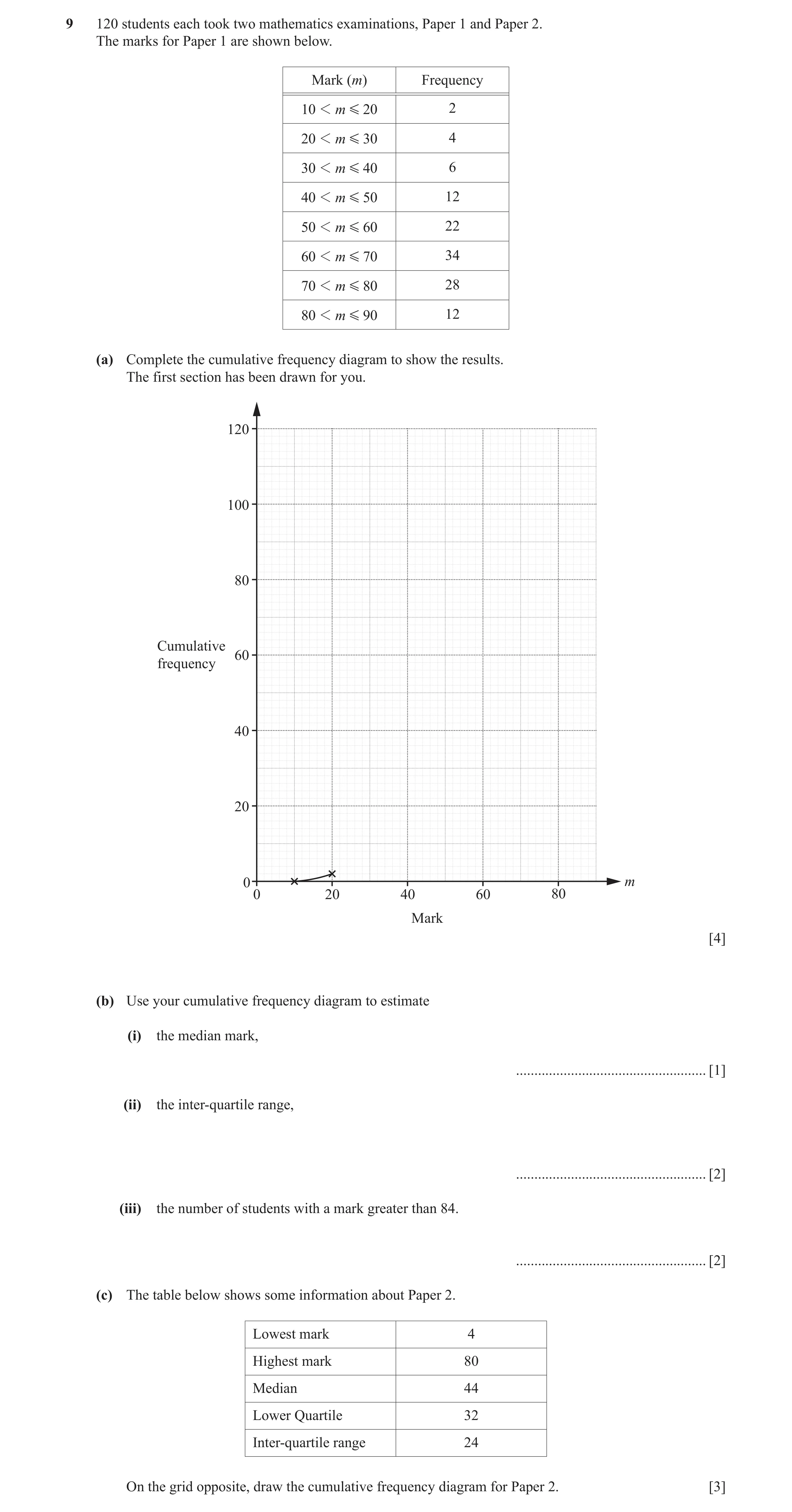
9 120 students each took two mathematics examinations, Paper 1 and Paper 2. The marks for Paper 1 are shown below. Mark (m) Frequency 10 1 m G 20 2 20 1 m G 30 4 30 1 m G 40 6 40 1 m G 50 12 50 1 m G 60 22 60 1 m G 70 34 70 1 m G 80 28 80 1 m G 90 12 (a) Complete the cumulative frequency diagram to show the results. The first section has been drawn for you. 120 100 80 Cumulative 60 frequency 40 20 0 m 0 20 40 60 80 Mark [4] (b) Use your cumulative frequency diagram to estimate (i) the median mark, … [1] (ii) the inter-quartile range, … [2] (iii) the number of students with a mark greater than 84. … [2] (c) The table below shows some information about Paper 2. Lowest mark 4 Highest mark 80 Median 44 Lower Quartile 32 Inter-quartile range 24 On the grid opposite, draw the cumulative frequency diagram for Paper 2. [3]
12 marks
Mark scheme: 9(a) Correct cf curve through 7 more 4 B3 for curve through 5 or more correct points points or B2 for curve through 4 correct points or correct cfs 2, 6, 12, 24, 46, 80, 108, 120 or B1 for curve through 3 correct points or 5,6 or 7 cfs 9(b)(i) 63 to 66 1 Only from increasing diagram 9(b)(ii) 17 to 23 2 B1 for LQ = 52 to 55 or UQ = 72 to 75 Only from increasing diagram 9(b)(iii) 4 to 8 2 B1 for 112 to 116 seen Only from increasing diagram 9(c) Correct cumulative frequency curve 3 B1 for lowest and highest points plotted correctly B1for median and lower quartile plotted correctly B1for upper quartile plotted correctly Maximum 2 marks if points not joined
This question in 0607/42 Oct/Nov 2018
Q4 · Rani planted some seeds in her garden 0607/41 May/June 2019
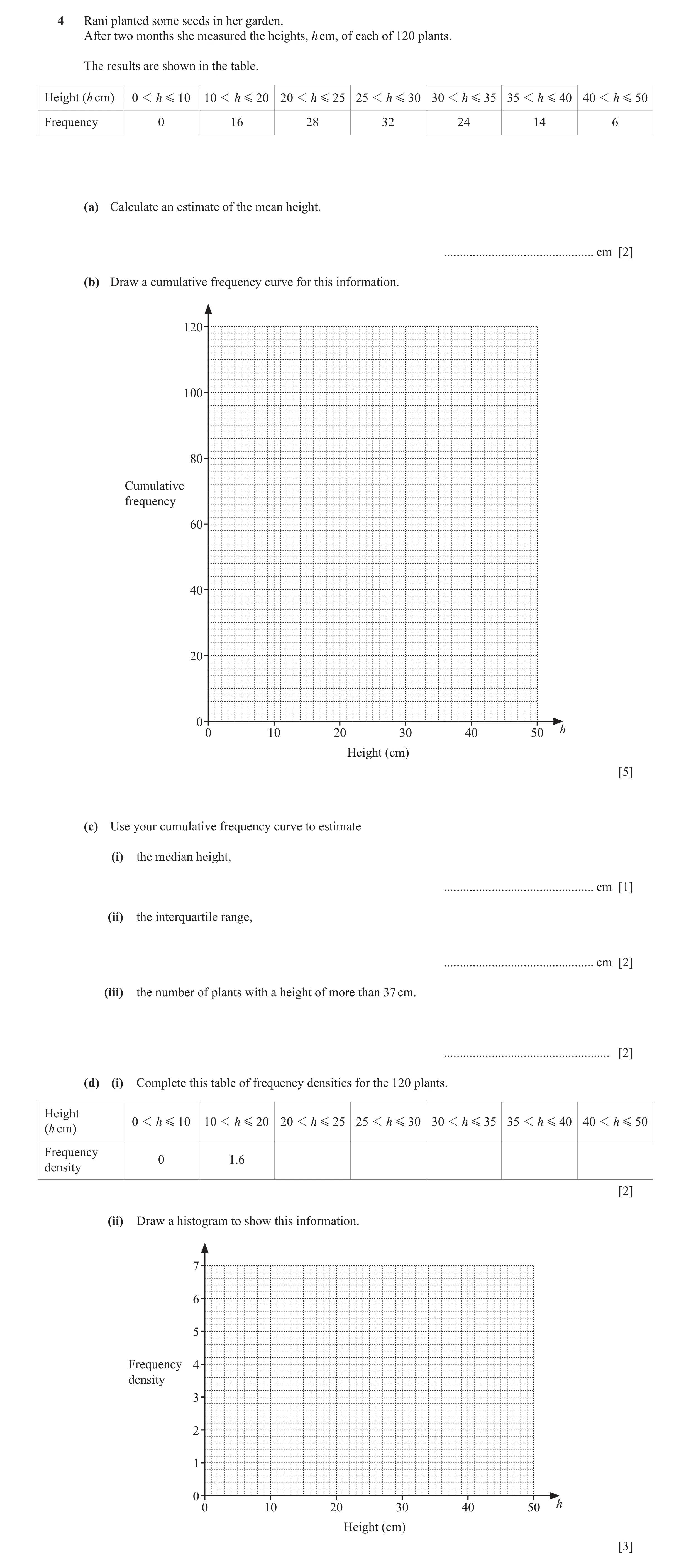
4 Rani planted some seeds in her garden. After two months she measured the heights, h cm, of each of 120 plants. The results are shown in the table. Height (h cm) 0 1 h G 10 10 1 h G 20 20 1 h G 25 25 1 h G 30 30 1 h G 35 35 1 h G 40 40 1 h G 50 Frequency 0 16 28 32 24 14 6 (a) Calculate an estimate of the mean height. … cm [2] (b) Draw a cumulative frequency curve for this information. 120 100 80 Cumulative frequency 60 40 20 0 h 0 10 20 30 40 50 Height (cm) [5] (c) Use your cumulative frequency curve to estimate (i) the median height, … cm [1] (ii) the interquartile range, … cm [2] (iii) the number of plants with a height of more than 37 cm. … [2] (d) (i) Complete this table of frequency densities for the 120 plants. Height 0 1 h G 10 10 1 h G 20 20 1 h G 25 25 1 h G 30 30 1 h G 35 35 1 h G 40 40 1 h G 50(h cm) Frequency 0 1.6density [2] (ii) Draw a histogram to show this information. 7 6 5 Frequency 4 density 3 2 1 0 h 0 10 20 30 40 50 Height (cm) [3]
17 marks
Mark scheme: 4(a) 27.7 or 27.70 to 27.71 2 M1 for at least 3 midpoints soi 4(b) Correct cf curve 5 Curve/polygon through (10, 0), (20, 16), (25, 44), (30, 76), (35, 100), (40, 114), (50, 120) or B4 for curve through 5 or 6 points or 7 points with no curve or B3 for 'correct curve' through all other consistent points in interval or B2 for all correct cfs or B1 for 4 or 5 correct cfs. If 0 scored SC1 for any cumulative frequency diagram. 4(c)(i) 26 to 28 1 Dep on increasing curve FT 4(c)(ii) 9 to 11.5 2 Dep on increasing curve FT B1 for lq = 22 to 23.5 or uq = 32.5 to 33.5 4(c)(iii) 10 to 15 2 Dep on increasing curve FT B1 for 105 to 110 seen 4(d)(i) 5.6, 6.4, 4.8, 2.8, 0.6 2 B1 for 3 or 4 correct 4(d)(ii) Correct histogram 3 B2 FT for bars with their heights or B1FT for 3 or 4 bars with their heights or bars with all correct widths
This question in 0607/41 May/June 2019
Q5 · 200 people took part in a charity walk 0607/41 Oct/Nov 2019
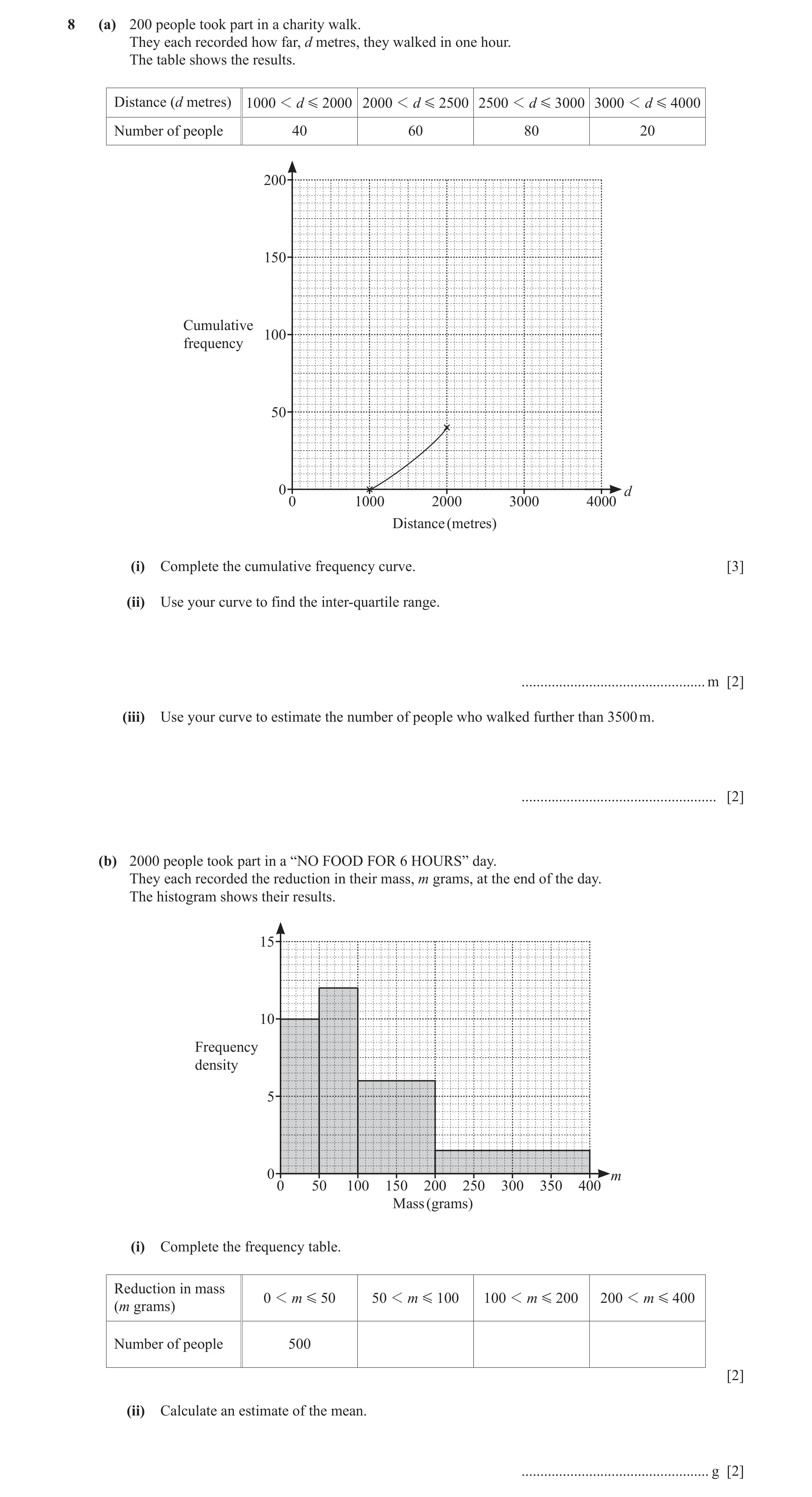
8 (a) 200 people took part in a charity walk. They each recorded how far, d metres, they walked in one hour. The table shows the results. Distance (d metres) 1000 1 d G 2000 2000 1 d G 2500 2500 1 d G 3000 3000 1 d G 4000 Number of people 40 60 80 20 200 150 Cumulative 100 frequency 50 0 d 0 1000 2000 3000 4000 Distance (metres) (i) Complete the cumulative frequency curve. [3] (ii) Use your curve to find the inter-quartile range. … m [2] (iii) Use your curve to estimate the number of people who walked further than 3500 m. … [2] (b) 2000 people took part in a “NO FOOD FOR 6 HOURS” day. They each recorded the reduction in their mass, m grams, at the end of the day. The histogram shows their results. 15 10 Frequency density 5 0 m 0 50 100 150 200 250 300 350 400 Mass (grams) (i) Complete the frequency table. Reduction in mass 0 1 m G 50 50 1 m G 100 100 1 m G 200 200 1 m G 400 (m grams) Number of people 500 [2] (ii) Calculate an estimate of the mean. … g [2]
11 marks
Mark scheme: 8(a)(i) Correct curve 3 B2 for two of (2500, 100), (3000, 180), (4000, 200) plotted or B1 for 100, 180, 200 soi 8(a)(ii) 600 to 700 2 B1 for [u.q.=] 2750 to 2800 or [l.q. = ] 2100 to 2150 not as final answer 8(a)(iii) 5 to 15 2 B1 for 185 to 195 seen 8(b)(i) 600, 600, 300 2 B1 for two correct 8(b)(ii) 118.75 2 M1 for at least two of 25 × 500 + 75 × their 600 + 150 × their 600 + 300 × their 300
This question in 0607/41 Oct/Nov 2019
Q6 · These are Tom’s ten homework marks 0607/41 May/June 2020
2 (a) These are Tom’s ten homework marks. 8 7 10 8 9 5 8 10 6 8 Find (i) the range, … [1] (ii) the mean, … [1] (iii) the median, … [1] (iv) the upper quartile. … [1] (b) The mass, m kg, of each of 120 parcels is recorded. The cumulative frequency curve shows the results. 120 100 80 Cumulative 60 frequency 40 20 0 m 0 0.5 1 1.5 2 2.5 3 3.5 4 Mass (kg) (i) Find the median. … kg [1] (ii) Find the lower quartile. … kg [1] (iii) Find the interquartile range. … kg [1] (iv) Find the number of parcels with a mass of more than 3 kg. … [2] (v) (a) Use the cumulative frequency curve to complete the frequency table. Mass (m kg) 0 1 m G 1 1 1 m G 1. 5 1.5 1 m G 2 2 1 m G 3 3 1 m G 4 Frequency 30 30 [3] (b) Use the frequency table to calculate an estimate of the mean. … kg [2]
14 marks
This question in 0607/41 May/June 2020
Q7 · The cumulative frequency graph shows the heights, in centimetres, of 120 plants in… 0607/43 May/June 2020
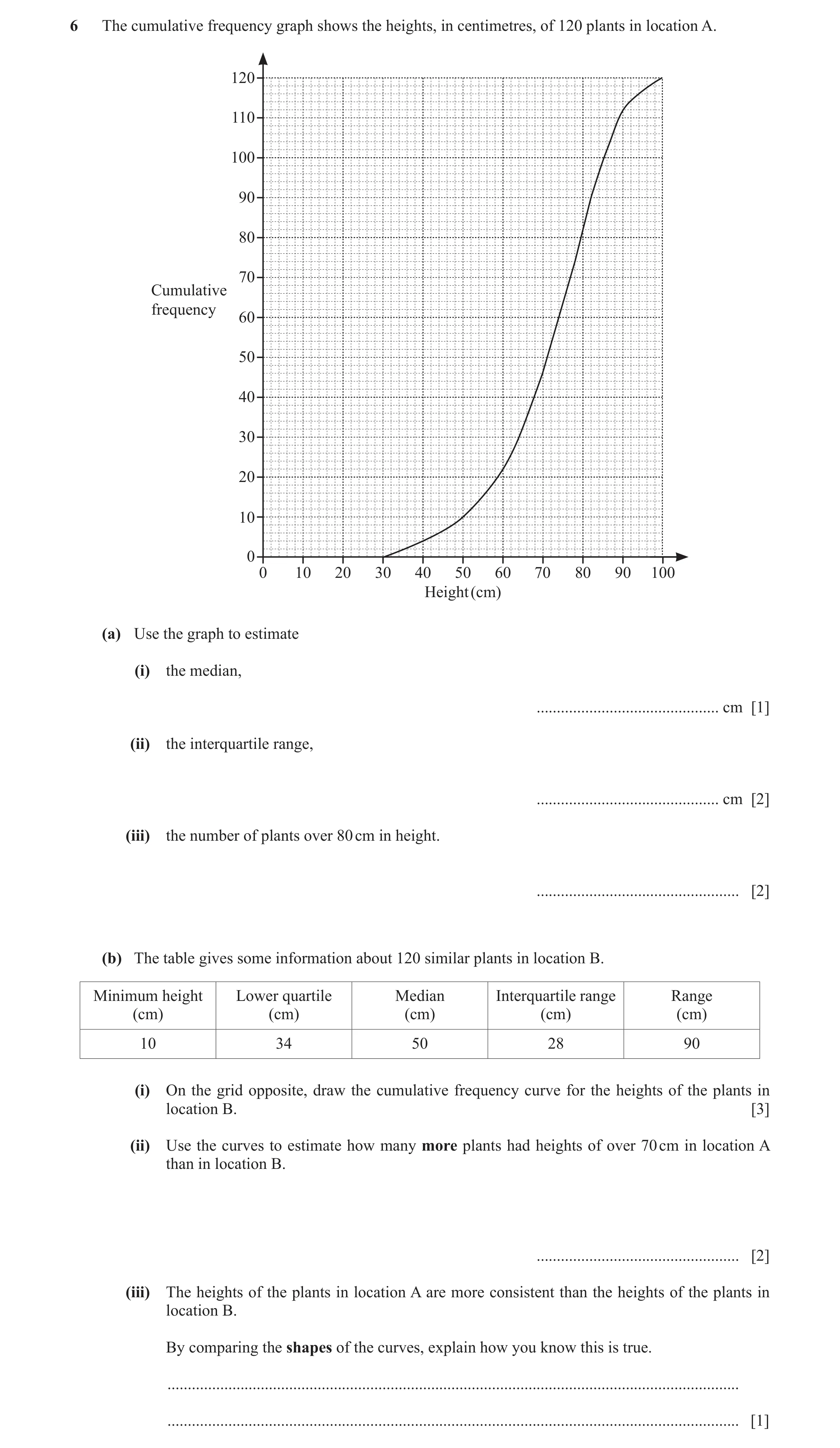
6 The cumulative frequency graph shows the heights, in centimetres, of 120 plants in location A. 120 110 100 90 80 70 Cumulative frequency 60 50 40 30 20 10 0 0 10 20 30 40 50 60 70 80 90 100 Height (cm) (a) Use the graph to estimate (i) the median, … cm [1] (ii) the interquartile range, … cm [2] (iii) the number of plants over 80 cm in height. … [2] (b) The table gives some information about 120 similar plants in location B. Minimum height Lower quartile Median Interquartile range Range (cm) (cm) (cm) (cm) (cm) 10 34 50 28 90 (i) On the grid opposite, draw the cumulative frequency curve for the heights of the plants in location B. [3] (ii) Use the curves to estimate how many more plants had heights of over 70 cm in location A than in location B. … [2] (iii) The heights of the plants in location A are more consistent than the heights of the plants in location B. By comparing the shapes of the curves, explain how you know this is true. … … [1]
11 marks
Mark scheme: 6(a)(ii) 18 2 B1 for 64 or 82 6(a)(iii) 38 2 B1 for 82 6(b)(i) Correct graph 3 B1 for minimum at (10, h) where h < 30, lq and median correct B1 for uq correct B1 for maximum correct 6(b)(ii) Answer in range 50 to 60 2 B1 for 74 or 14 to 24 6(b)(iii) [A is] steeper oe 1
This question in 0607/43 May/June 2020
Q8 · The mass, m grams, of each of 50 apples is found 0607/42 Feb/March 2021
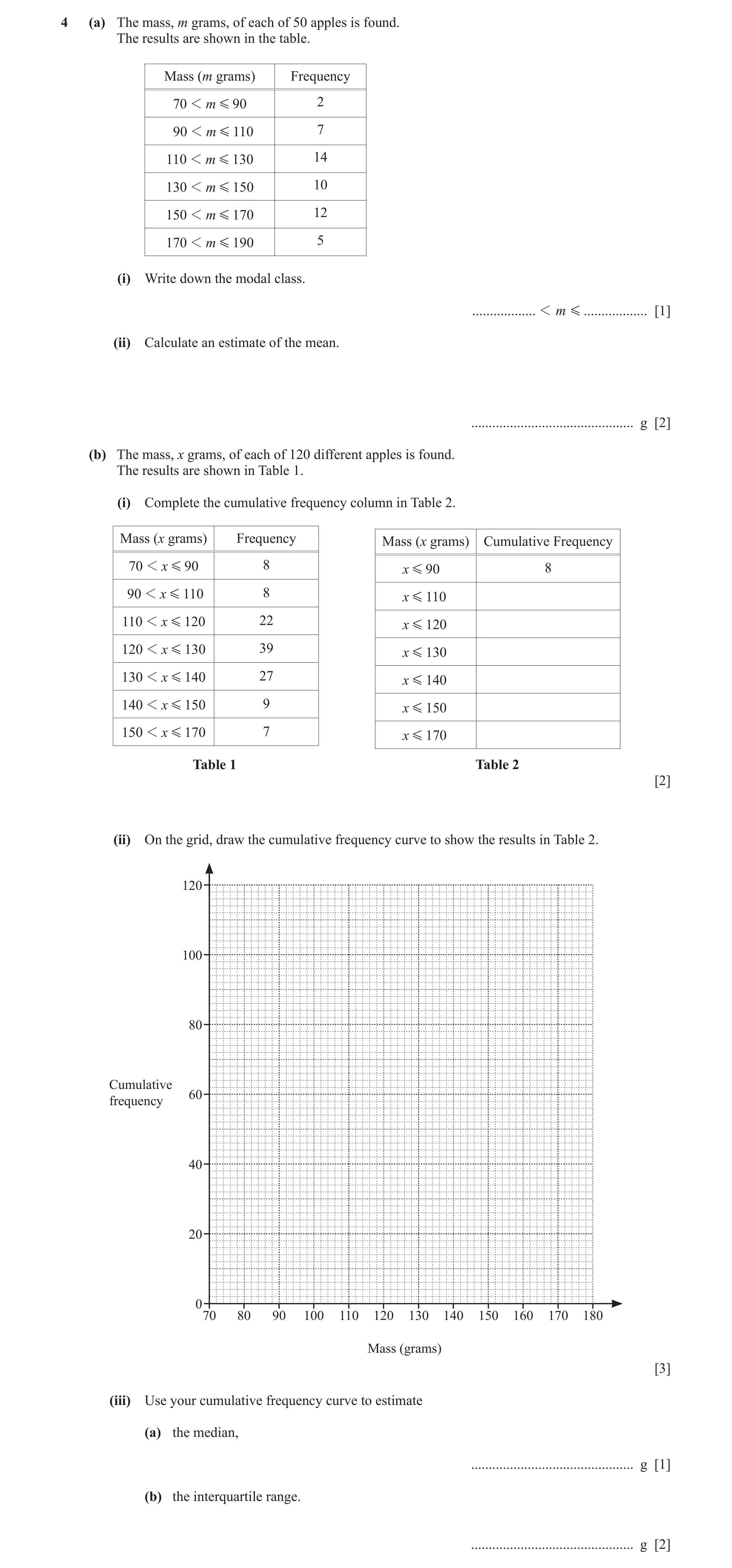
4 (a) The mass, m grams, of each of 50 apples is found. The results are shown in the table. Mass (m grams) Frequency 70 1 m G 90 2 90 1 m G 110 7 110 1 m G 130 14 130 1 m G 150 10 150 1 m G 170 12 170 1 m G 190 5 (i) Write down the modal class. … 1 m G … [1] (ii) Calculate an estimate of the mean. … g [2] (b) The mass, x grams, of each of 120 different apples is found. The results are shown in Table 1. (i) Complete the cumulative frequency column in Table 2. Mass (x grams) Frequency Mass (x grams) Cumulative Frequency 70 1 x G 90 8 x G 90 8 90 1 x G 110 8 x G 110 110 1 x G 120 22 x G 120 120 1 x G 130 39 x G 130 130 1 x G 140 27 x G 140 140 1 x G 150 9 x G 150 150 1 x G 170 7 x G 170 Table 1 Table 2 [2] (ii) On the grid, draw the cumulative frequency curve to show the results in Table 2. 120 100 80 Cumulative 60frequency 40 20 0 70 80 90 100 110 120 130 140 150 160 170 180 Mass (grams) [3] (iii) Use your cumulative frequency curve to estimate (a) the median, … g [1] (b) the interquartile range. … g [2]
11 marks
Mark scheme: 4(a)(i) 110 < m ≤ 130 1 4(a)(ii) 135.2 2 M1 for mid-values seen or implied 4(b)(i) (8) 16 38 77 104 113 120 2 B1 for 4 or 5 correct FT one error 4(b)(ii) Correct cumulative frequency 3 B2 for 6 points correct curve OR B1FT for 7 heights correct B1 for plotting at upper boundary of interval 4(b)(iii)(a) 124 to 127 nfww 1 4(b)(iii)(b) 14 to 21 2 B1 for [LQ =] 115 to 118 or [UQ =] 132 to 136
This question in 0607/42 Feb/March 2021
Q9 · The marks, x, of 300 students in a chemistry test are shown in the table 0607/41 May/June 2021
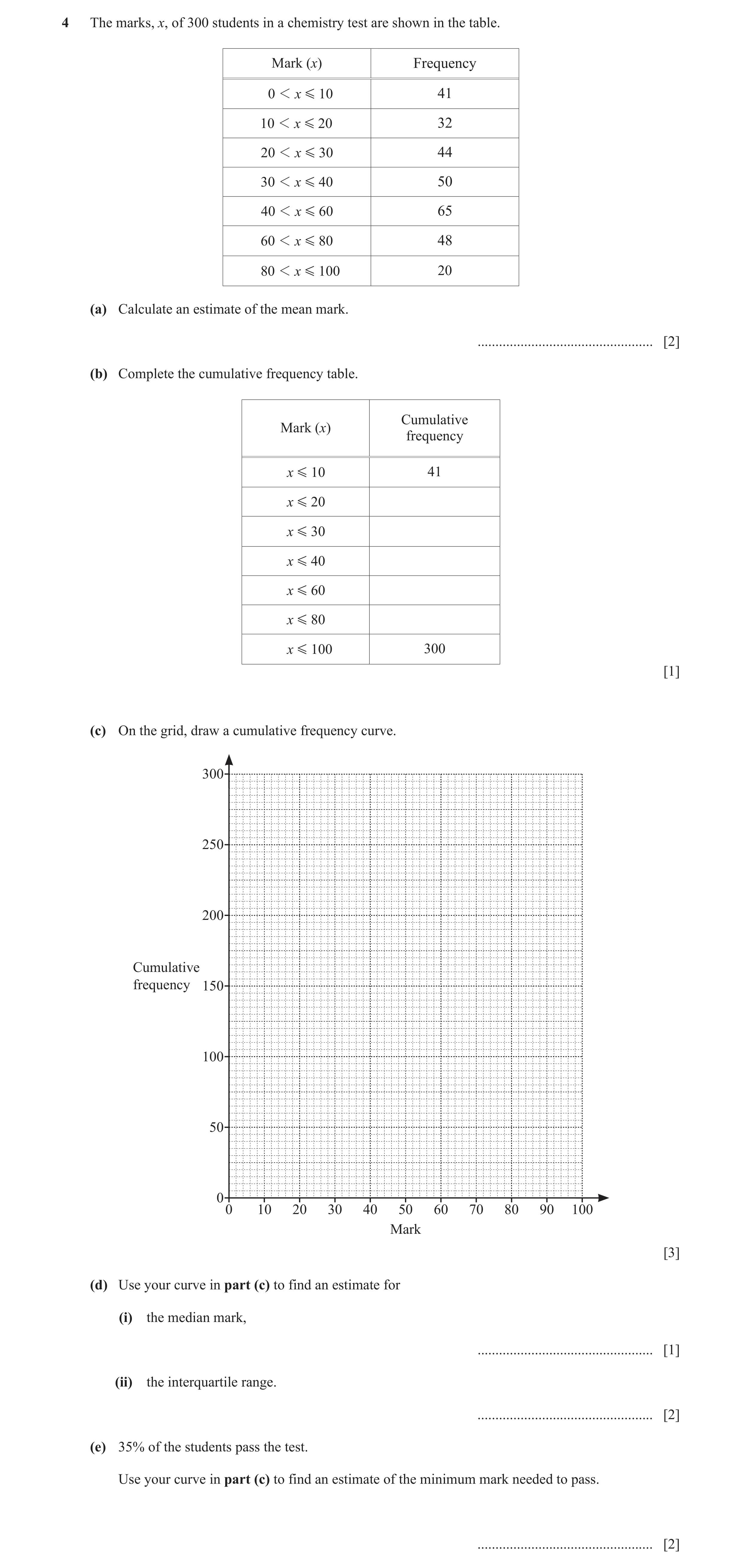
4 The marks, x, of 300 students in a chemistry test are shown in the table. Mark (x) Frequency 0 1 x G 10 41 10 1 x G 20 32 20 1 x G 3 0 44 30 1 x G 40 50 40 1 x G 60 65 60 1 x G 8 0 48 80 1 x G 100 20 (a) Calculate an estimate of the mean mark. … [2] (b) Complete the cumulative frequency table. Cumulative Mark (x) frequency x G 10 41 x G 20 x G 30 x G 40 x G 60 x G 80 x G 100 300 [1] (c) On the grid, draw a cumulative frequency curve. 300 250 200 Cumulative frequency 150 100 50 0 0 10 20 30 40 50 60 70 80 90 100 Mark [3] (d) Use your curve in part (c) to find an estimate for (i) the median mark, … [1] (ii) the interquartile range. … [2] (e) 35% of the students pass the test. Use your curve in part (c) to find an estimate of the minimum mark needed to pass. … [2]
11 marks
Mark scheme: 4(a) 39.8 or 39.81 to 39.82 2 M1 for at least 5 correct mid-points soi 4(b) [41], 73, 117, 167, 232, 280, [300] 1 In parts (c), (d) and (e), marks can only be earned with an increasing curve 4(c) Correct curve 3 M1 for horizontal plot correct (10, 41) (20, 73) (30, 117) (40, 167) M1 for at least 6 vertical plots from their (60, 232) (80, 280) (100, 300) table correct 4(d)(i) 35 to 38 1 4(d)(ii) 35 to 39 2 B1 for [UQ =] 56 to 59 or [LQ =] 20 to 21 4(e) 46 to 50 2 B1 for 195 or 105 seen
This question in 0607/41 May/June 2021
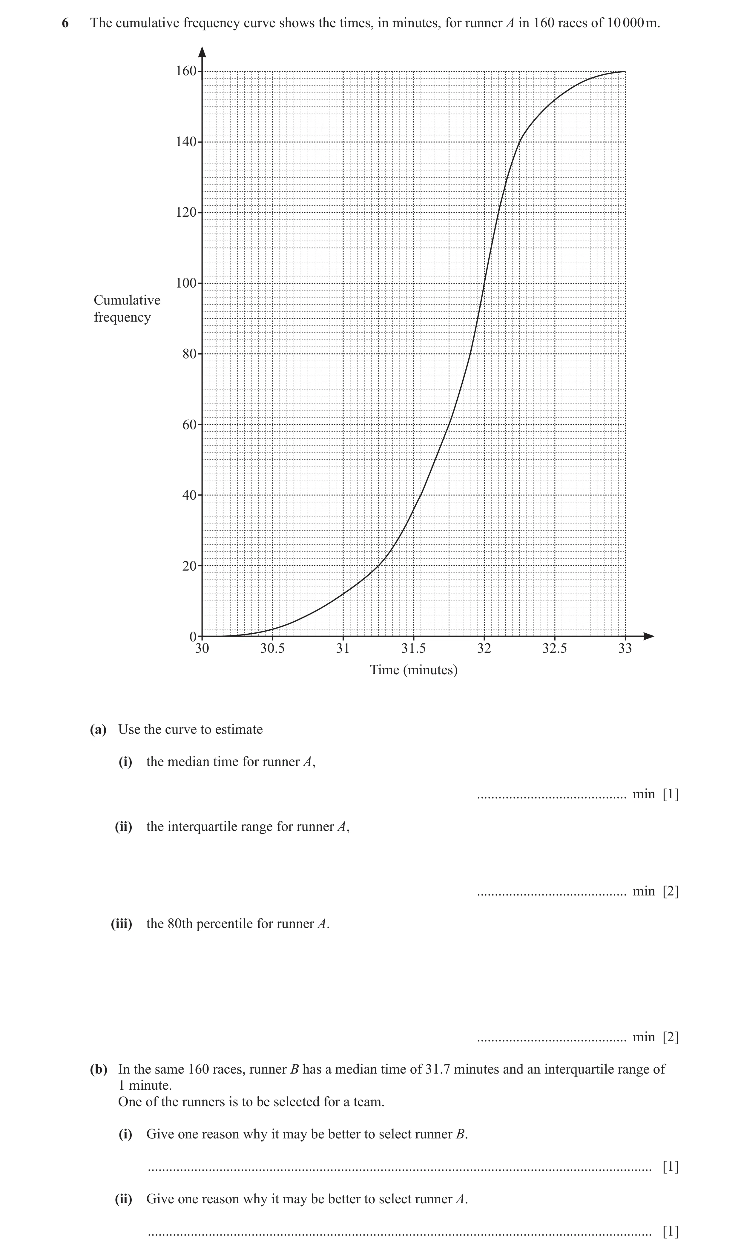
Q10 · The cumulative frequency curve shows the times, in minutes, for runner A in 160 races of… 0607/42 May/June 2021
6 The cumulative frequency curve shows the times, in minutes, for runner A in 160 races of 10 000 m. 160 140 120 100 Cumulative frequency 80 60 40 20 0 30 30.5 31 31.5 32 32.5 33 Time (minutes) (a) Use the curve to estimate (i) the median time for runner A, … min [1] (ii) the interquartile range for runner A, … min [2] (iii) the 80th percentile for runner A. … min [2] (b) In the same 160 races, runner B has a median time of 31.7 minutes and an interquartile range of 1 minute. One of the runners is to be selected for a team. (i) Give one reason why it may be better to select runner B. … [1] (ii) Give one reason why it may be better to select runner A. … [1]
7 marks
Mark scheme: 6(a)(i) 31.9 1 6(a)(ii) 0.55 2 M1 for [UQ =] 32.1 or [LQ =] 31.55 seen 6(a)(iii) 32.15 2 B1 for 128 seen 6(b)(i) Lower median (average) oe 1 6(b)(ii) Smaller IQR oe 1
This question in 0607/42 May/June 2021
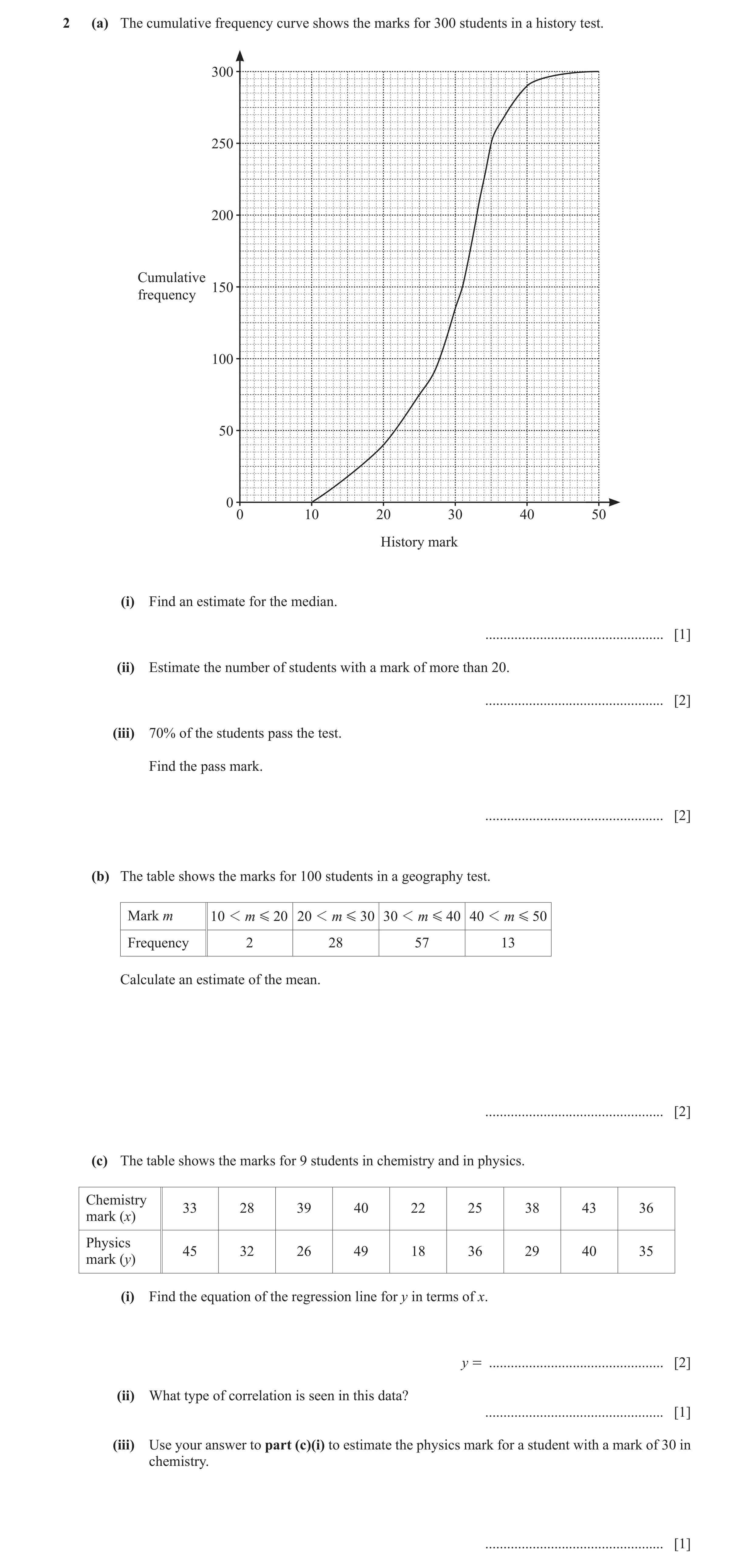
Q11 · The cumulative frequency curve shows the marks for 300 students in a history test 0607/41 May/June 2022
2 (a) The cumulative frequency curve shows the marks for 300 students in a history test. 300 250 200 Cumulative 150 frequency 100 50 0 0 10 20 30 40 50 History mark (i) Find an estimate for the median. … [1] (ii) Estimate the number of students with a mark of more than 20. … [2] (iii) 70% of the students pass the test. Find the pass mark. … [2] (b) The table shows the marks for 100 students in a geography test. Mark m 10 1 m G 20 20 1 m G 30 30 1 m G 40 40 1 m G 50 Frequency 2 28 57 13 Calculate an estimate of the mean. … [2] (c) The table shows the marks for 9 students in chemistry and in physics. Chemistry 33 28 39 40 22 25 38 43 36mark (x) Physics 45 32 26 49 18 36 29 40 35mark (y) (i) Find the equation of the regression line for y in terms of x. y = … [2] (ii) What type of correlation is seen in this data? … [1] (iii) Use your answer to part (c)(i) to estimate the physics mark for a student with a mark of 30 in chemistry. … [1]
11 marks
Mark scheme: 2(a)(i) 31 1 2(a)(ii) 260 2 B1 for 40 seen 2(a)(iii) 27 2 70 30 M1 for 300 soi or 300 100 100 2(b) 33.1 2 M1 for at least three mid-values soi 2(c)(i) y 0.618 x 13.6 2 B1 for 0.618x + k or kx + 13.6 or 0.62x + 14 2(c)(ii) positive 1 2(c)(iii) 32 or 32.0 to 32.6 1 FT their (c)(i) if linear eqn
This question in 0607/41 May/June 2022
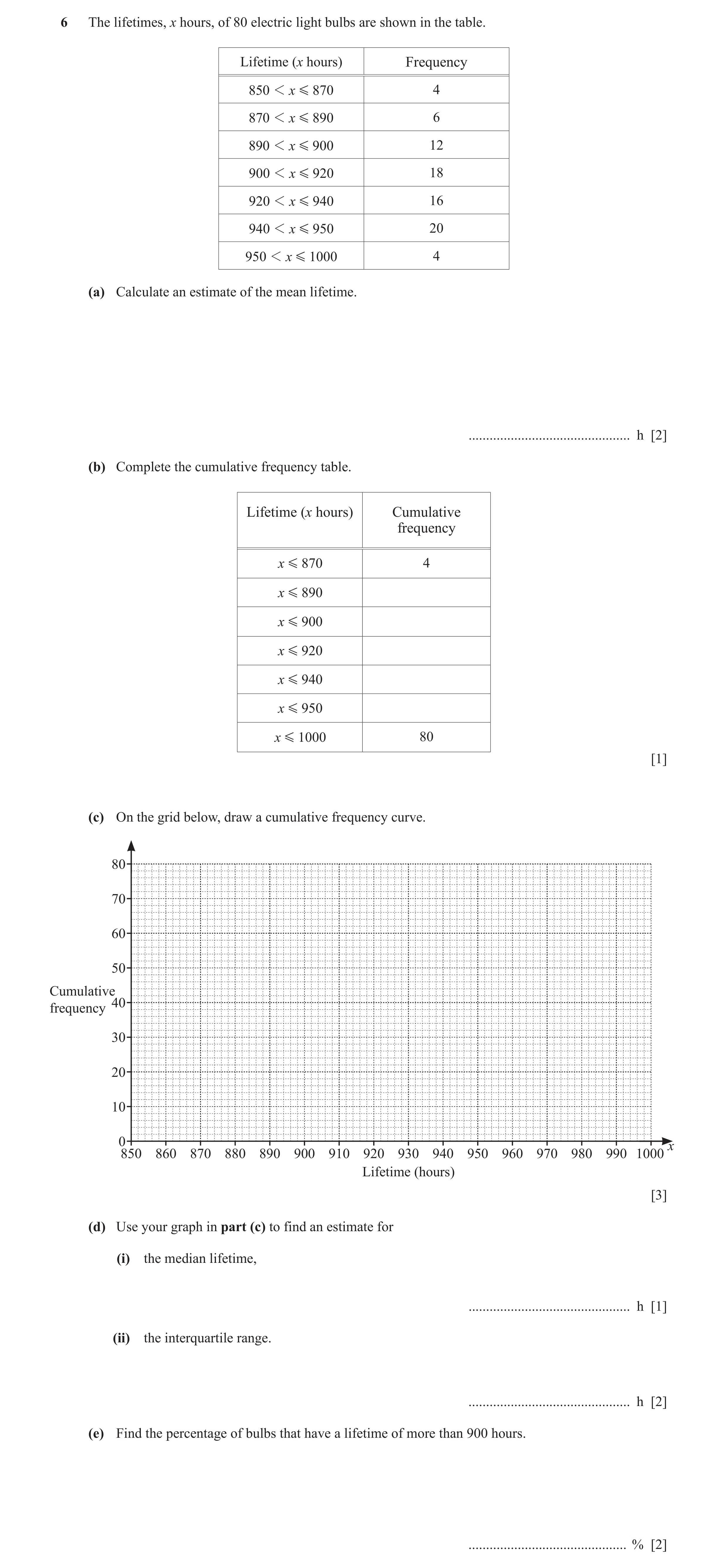
Q12 · The lifetimes, x hours, of 80 electric light bulbs are shown in the table 0607/42 May/June 2022
6 The lifetimes, x hours, of 80 electric light bulbs are shown in the table. Lifetime (x hours) Frequency 850 1 x G 870 4 870 1 x G 890 6 890 1 x G 900 12 900 1 x G 920 18 920 1 x G 940 16 940 1 x G 950 20 950 1 x G 1000 4 (a) Calculate an estimate of the mean lifetime. … h [2] (b) Complete the cumulative frequency table. Lifetime (x hours) Cumulative frequency x G 870 4 x G 890 x G 900 x G 920 x G 940 x G 950 x G 1000 80 [1] (c) On the grid below, draw a cumulative frequency curve. 80 70 60 50 Cumulative 40frequency 30 20 10 0 x 850 860 870 880 890 900 910 920 930 940 950 960 970 980 990 1000 Lifetime (hours) [3] (d) Use your graph in part (c) to find an estimate for (i) the median lifetime, … h [1] (ii) the interquartile range. … h [2] (e) Find the percentage of bulbs that have a lifetime of more than 900 hours. … % [2]
11 marks
Mark scheme: 6(a) 919 2 M1 for at least 5 correct midpoints soi 6(b) [ 4], 10, 22, 40, 56, 76, [80] 1 6(c) Correct curve or polygon and correct points 3 M1 for at least 6 horizontal plots correct plotted M1FT for at least 6 vertical plots correct (870, 4) (890, 10) (900, 22) (920, 40) (940, 56) (950, 76) (1000, 80) 6(d)(i) 920 1 6(d)(ii) 42 to 47 2 M1FT for [UQ =] 941 to 944 or [LQ =] 897 to 899 6(e) 72.5 2 B1 for 18+16+20+4 or 80 – 22 soi (58) or M1 for (80 – their 22)/80 × 100
This question in 0607/42 May/June 2022
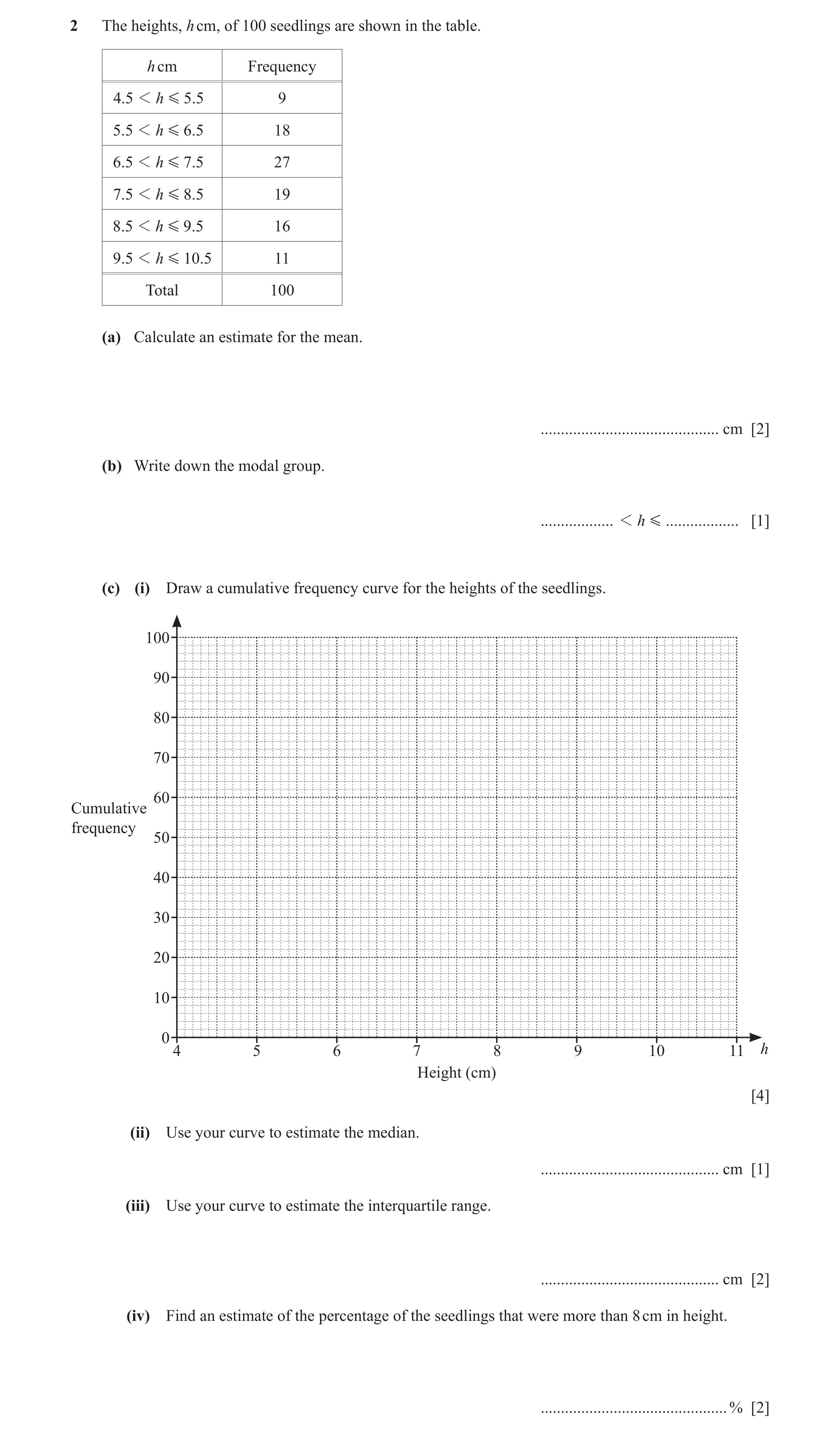
Q13 · The heights, h cm, of 100 seedlings are shown in the table 0607/43 May/June 2022
2 The heights, h cm, of 100 seedlings are shown in the table. h cm Frequency 4.5 1 h G 5.5 9 5.5 1 h G 6.5 18 6.5 1 h G 7 .5 27 7.5 1 h G 8.5 19 8.5 1 h G 9.5 16 9.5 1 h G 10.5 11 Total 100 (a) Calculate an estimate for the mean. … cm [2] (b) Write down the modal group. … 1 h G … [1] (c) (i) Draw a cumulative frequency curve for the heights of the seedlings. 100 90 80 70 60Cumulative frequency 50 40 30 20 10 0 4 5 6 7 8 9 10 11 h Height (cm) [4] (ii) Use your curve to estimate the median. … cm [1] (iii) Use your curve to estimate the interquartile range. … cm [2] (iv) Find an estimate of the percentage of the seedlings that were more than 8 cm in height. … % [2]
12 marks
Mark scheme: 2(a) 7.48 2 M1 for evidence of mid-values 2(b) 6.5 7.5 1 2(c)(i) Correct cf curve through 6 points 4 B3 for curve through 5 correct points or B2 for curve through 4 correct points or correct cfs [9], 27, 54, 73, 89, 100 or B1 for curve through 4 correct points or 3, 4 or 5 cfs 2(c)(ii) 7.2 to 7.4 1 FT Only from increasing diagram 2(c)(iii) 2.0 to 2.4 2 B1FT for lq = 6.3 to 6.5 or uq = 8.5 to 8.7 FT only from increasing diagram 2(c)(iv) 34 to 38 2 B1 FT for 62 to 66 seen
This question in 0607/43 May/June 2022
Q14 · The cumulative frequency table shows the masses, in grams, of 1200 potatoes 0607/41 Oct/Nov 2022
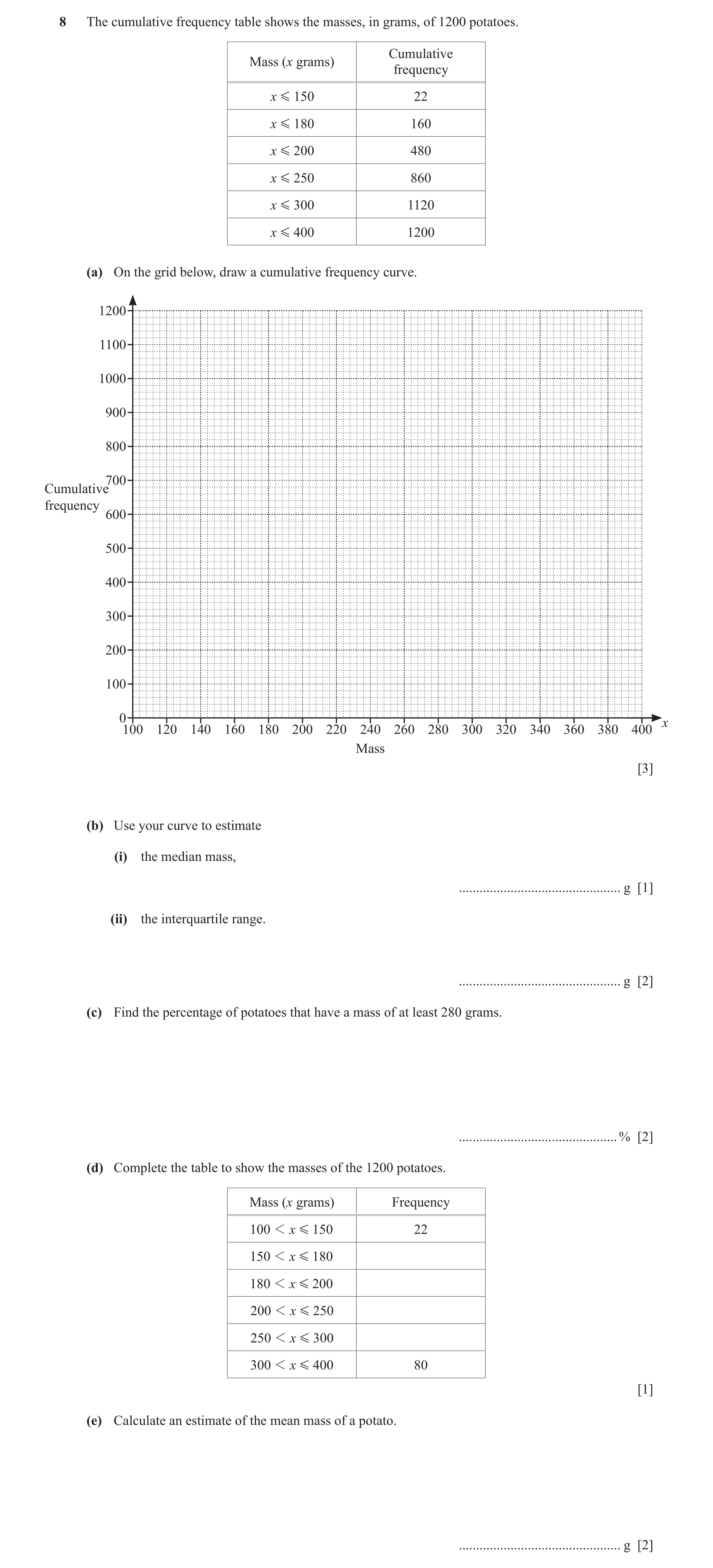
8 The cumulative frequency table shows the masses, in grams, of 1200 potatoes. Cumulative Mass (x grams) frequency x G 150 22 x G 180 160 x G 200 480 x G 250 860 x G 300 1120 x G 400 1200 (a) On the grid below, draw a cumulative frequency curve. 1200 1100 1000 900 800 700Cumulative frequency 600 500 400 300 200 100 0 x 100 120 140 160 180 200 220 240 260 280 300 320 340 360 380 400 Mass [3] (b) Use your curve to estimate (i) the median mass, … g [1] (ii) the interquartile range. … g [2] (c) Find the percentage of potatoes that have a mass of at least 280 grams. … % [2] (d) Complete the table to show the masses of the 1200 potatoes. Mass (x grams) Frequency 100 1 x G 150 22 150 1 x G 180 180 1 x G 200 200 1 x G 250 250 1 x G 300 300 1 x G 400 80 [1] (e) Calculate an estimate of the mean mass of a potato. … g [2]
11 marks
Mark scheme: 8(a) Correct curve 3 M1 for at least 5 horizontal plots correct (150, 22) (180, 160) (200, 480) M1 for at least 5 vertical plots correct (250, 860) (300, 1120) (400, 1200) 8(b)(i) 208 to 218 1 FT their curve 8(b)(ii) 55 to 75 2 M1FT for [UQ =] 250 to 260 or [LQ =] 185 to 195 seen 8(c) 12 to 17 2 1200 − their 1020 M1 for [100] 1200 their 1020 or 100 1200 8(d) [22], 138, 320, 380, 260, [80] 1 8(e) 226.1 or 226 2 M1 for at least four of 125, 165, 190, 225, 275, 350 soi
This question in 0607/41 Oct/Nov 2022
Q15 · The distance, d km, cycled by each of 120 cyclists was recorded 0607/42 Oct/Nov 2022
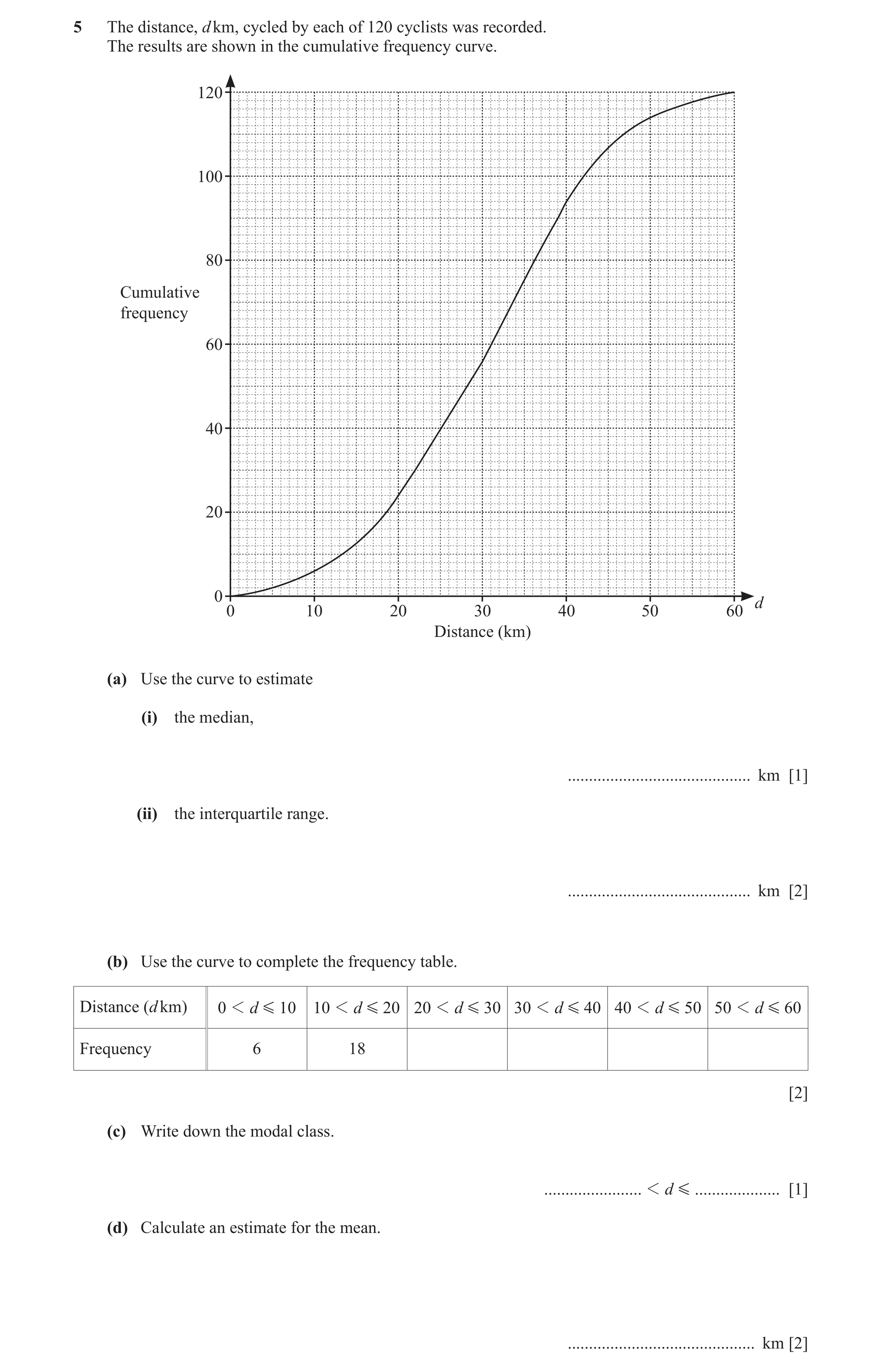
5 The distance, d km, cycled by each of 120 cyclists was recorded. The results are shown in the cumulative frequency curve. 120 100 80 Cumulative frequency 60 40 20 0 d 0 10 20 30 40 50 60 Distance (km) (a) Use the curve to estimate (i) the median, … km [1] (ii) the interquartile range. … km [2] (b) Use the curve to complete the frequency table. Distance (d km) 0 1 d G 10 10 1 d G 20 20 1 d G 30 30 1 d G 40 40 1 d G 50 50 1 d G 60 Frequency 6 18 [2] (c) Write down the modal class. … 1 d G … [1] (d) Calculate an estimate for the mean. … km [2]
8 marks
Mark scheme: 5(a)(i) 31 cao 1 5(a)(ii) 17 cao 2 B1 for [l.q. =] 22 or [u.q. =] 39 seen 5(b) 32, 38, 20, 6 2 B1 for 2 correct 5(c) 30 < d ⩽ 40 1 FT their table 5(d) 30.5 2 M1 for mid-points 5, 15, 25, ... soi
This question in 0607/42 Oct/Nov 2022
Q16 · The heights, x cm, of 500 students in a school are shown in the table 0607/42 Feb/March 2023
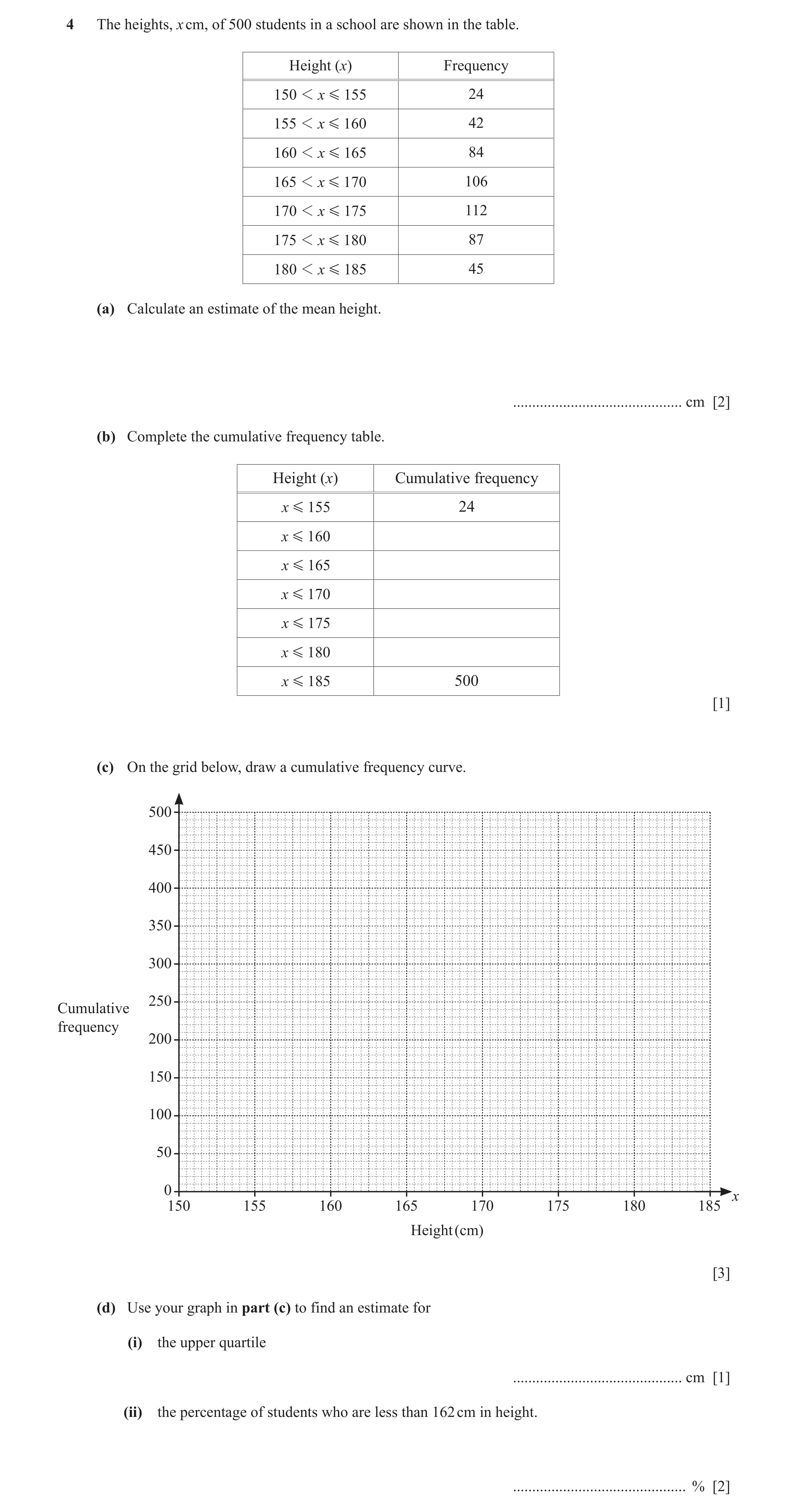
4 The heights, x cm, of 500 students in a school are shown in the table. Height (x) Frequency 150 1 x G 155 24 155 1 x G 160 42 160 1 x G 165 84 165 1 x G 170 106 170 1 x G 1 75 112 175 1 x G 180 87 180 1 x G 185 45 (a) Calculate an estimate of the mean height. … cm [2] (b) Complete the cumulative frequency table. Height (x) Cumulative frequency x G 155 24 x G 160 x G 165 x G 170 x G 175 x G 180 x G 185 500 [1] (c) On the grid below, draw a cumulative frequency curve. 500 450 400 350 300 250Cumulative frequency 200 150 100 50 0 x 150 155 160 165 170 175 180 185 Height (cm) [3] (d) Use your graph in part (c) to find an estimate for (i) the upper quartile … cm [1] (ii) the percentage of students who are less than 162 cm in height. … % [2]
9 marks
Mark scheme: 4(a) 169.31 or 169 or 169.3 2 M1 for use of mid-points e.g. 24 × 152.5 + 42×157.5 + 84 × 162.5 … 4(b) [24], 66, 150, 256, 368, 455, [500] 1 4(c) Correct curve 3 M1 for horizontal plot correct (155, 24) (160, 66) (165, 150) M1 for at least 5 vertical plots correct (170, 256) (175, 368) (180, 455) (185, 500) 4(d)(i) 175 to 176.5 1 FT their curve 4(d)(ii) 18 to 20 2 B1 for 90 to 100 their 90 or M1 for [ 100] soi 500
This question in 0607/42 Feb/March 2023
Q17 · The masses, m kg, of 160 students are recorded in the table 0607/42 May/June 2023
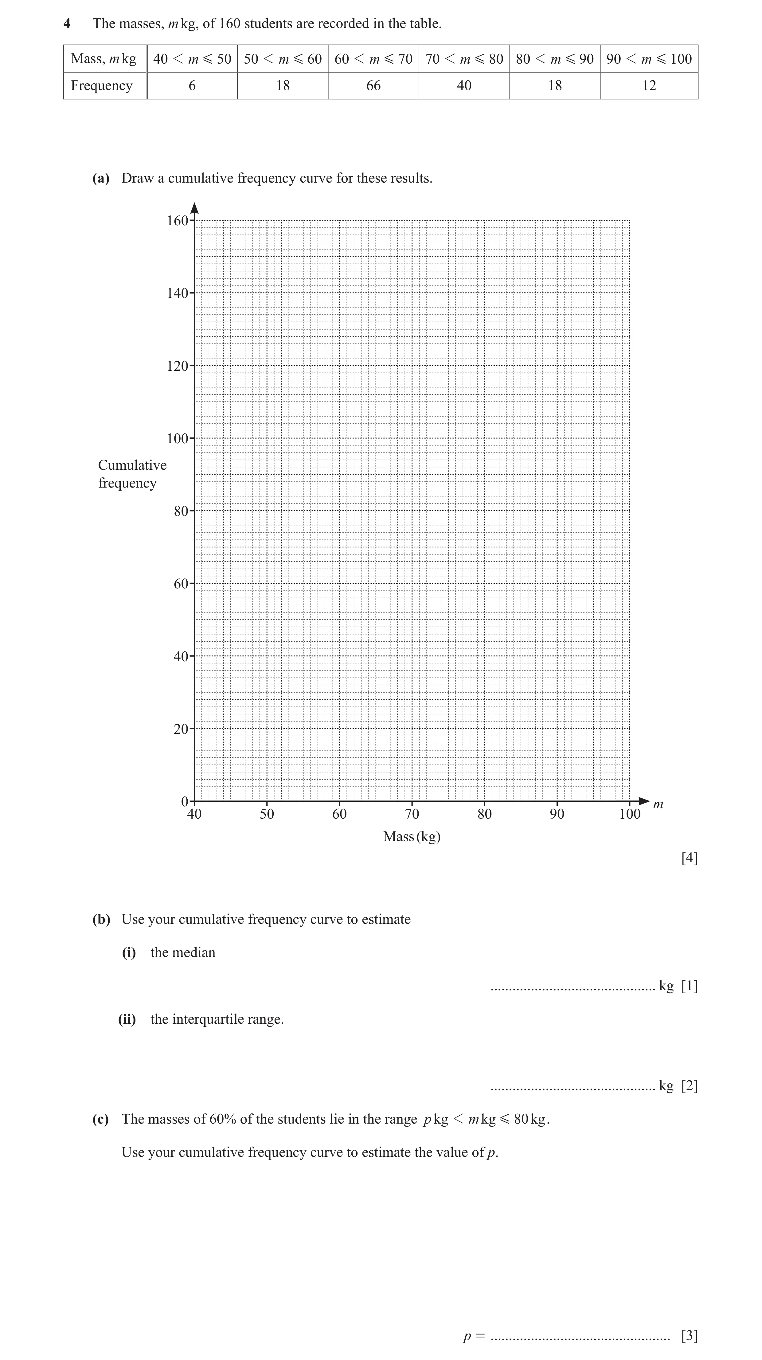
4 The masses, m kg, of 160 students are recorded in the table. Mass, m kg 40 1 m G 50 50 1 m G 60 60 1 m G 70 70 1 m G 80 80 1 m G 90 90 1 m G 100 Frequency 6 18 66 40 18 12 (a) Draw a cumulative frequency curve for these results. 160 140 120 100 Cumulative frequency 80 60 40 20 0 m 40 50 60 70 80 90 100 Mass (kg) [4] (b) Use your cumulative frequency curve to estimate (i) the median … kg [1] (ii) the interquartile range. … kg [2] (c) The masses of 60% of the students lie in the range p kg 1 m kg G 80 kg . Use your cumulative frequency curve to estimate the value of p. p = … [3]
10 marks
Mark scheme: 4(a) Correct cumulative frequency curve 4 B2 for 5 or 6 correct heights or B1 for 6, 24, 90, 130, 148, 160 soi B1 for points plotted at right hand end of interval. 4(b)(i) 66 to 69 1 FT their curve 4(b)(ii) 10 to 15 2 B1 for [lq] = 62 to 64 or [uq] = 74 to 77 FT their curve for B1 4(c) 61 to 63 nfww 3 B2 for 34 soi or M1 for 160 × 0.6 oe soi by 96
This question in 0607/42 May/June 2023
Q18 · Each of 200 students records their height, h cm 0607/41 Oct/Nov 2023
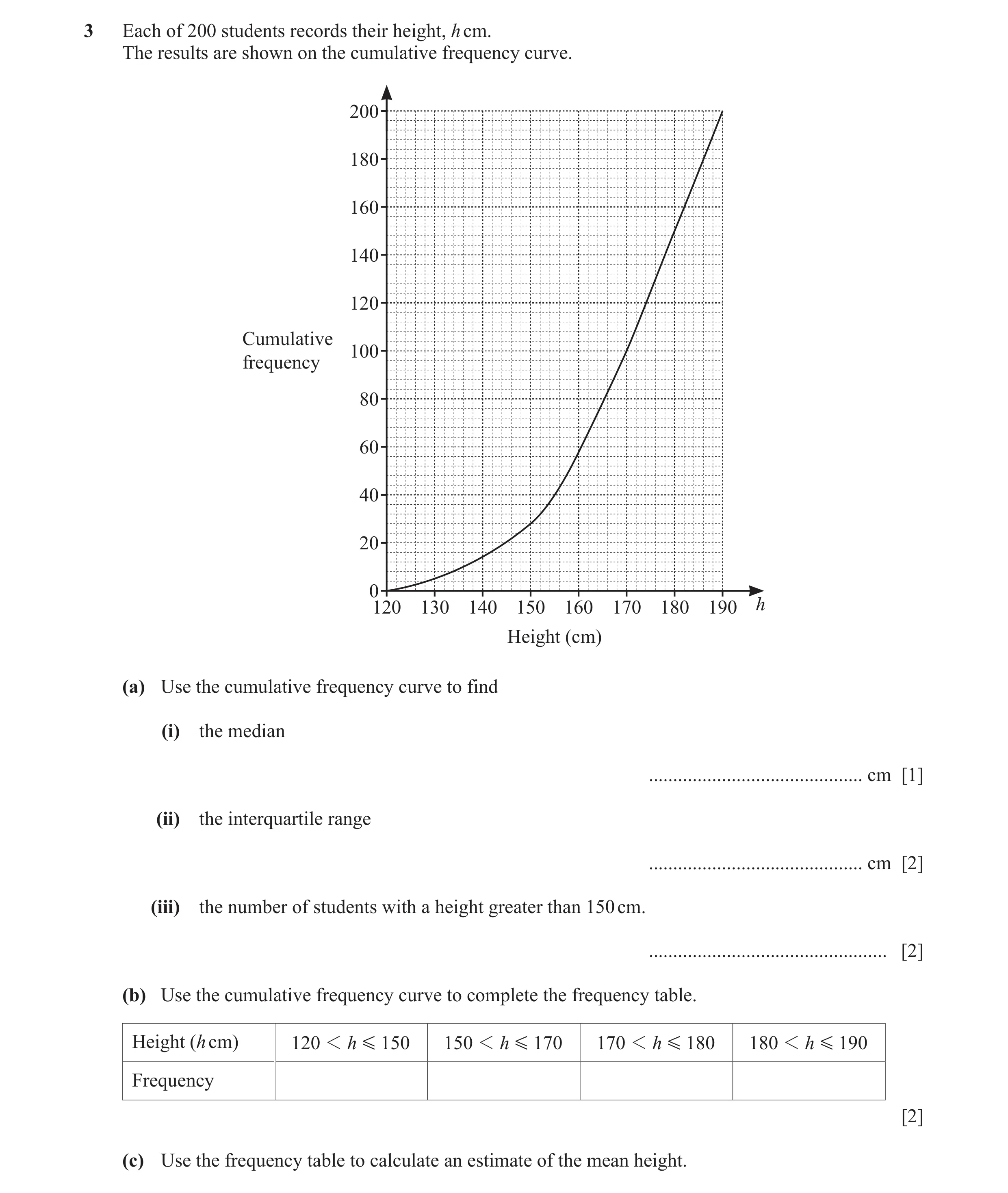
3 Each of 200 students records their height, h cm. The results are shown on the cumulative frequency curve. 200 180 160 140 120 Cumulative 100 frequency 80 60 40 20 0 120 130 140 150 160 170 180 190 h Height (cm) (a) Use the cumulative frequency curve to find (i) the median … cm [1] (ii) the interquartile range … cm [2] (iii) the number of students with a height greater than 150 cm. … [2] (b) Use the cumulative frequency curve to complete the frequency table. Height (h cm) 120 1 h G 150 150 1 h G 170 170 1 h G 180 180 1 h G 190 Frequency [2] (c) Use the frequency table to calculate an estimate of the mean height.
9 marks
Mark scheme: 3(a)(i) 170 1 3(a)(ii) 22 2 B1 for 158 or 180 seen 3(a)(iii) 172 2 B1 for 28 seen 3(b) 28, 72, 48 to 52, 52 to 48 2 B1 for two or three correct [total = 200] 3(c) 166.4 to 166.6 2 M1 for 3 or more mid-values soi
This question in 0607/41 Oct/Nov 2023
Q19 · 240 people take part in a marathon race 0607/43 Oct/Nov 2023
7 240 people take part in a marathon race. The times, t minutes, they took for the race are shown in the cumulative frequency curve. 240 220 200 180 160 140 Cumulative frequency 120 100 80 60 40 20 0 t 150 160 170 180 190 200 210 220 Time in minutes (a) Use the curve to estimate (i) the median time … min [1] (ii) the interquartile range. … min [2] (b) The fastest 20% of the runners are awarded a medal. Use the curve to estimate the longest time taken by a runner who received a medal. … min [2] (c) Use the curve to complete the frequency table. Time, 150 1 t G 160 160 1 t G 170 170 1 t G 180 180 1 t G 190 190 1 t G 200 200 1 t G 210 210 1 t G 220t minutes Frequency 16 32 [2] (d) Use the table in part (c) to calculate an estimate of the mean time. … min [2]
9 marks
Mark scheme: 7(a)(i) 182 1 7(a)(ii) 16 2 B1 for [uq=]189 or [lq=] 173 7(b) 170 2 B1 for 48 seen 7(c) 56, 84, 36, 12, 4 2 B1 for 3 or 4 correct 7(d) 181 2 M1 for at least 4 mid-points soi
This question in 0607/43 Oct/Nov 2023
Q20 · The table shows the money received in a shop for 120 days 0607/42 Feb/March 2024
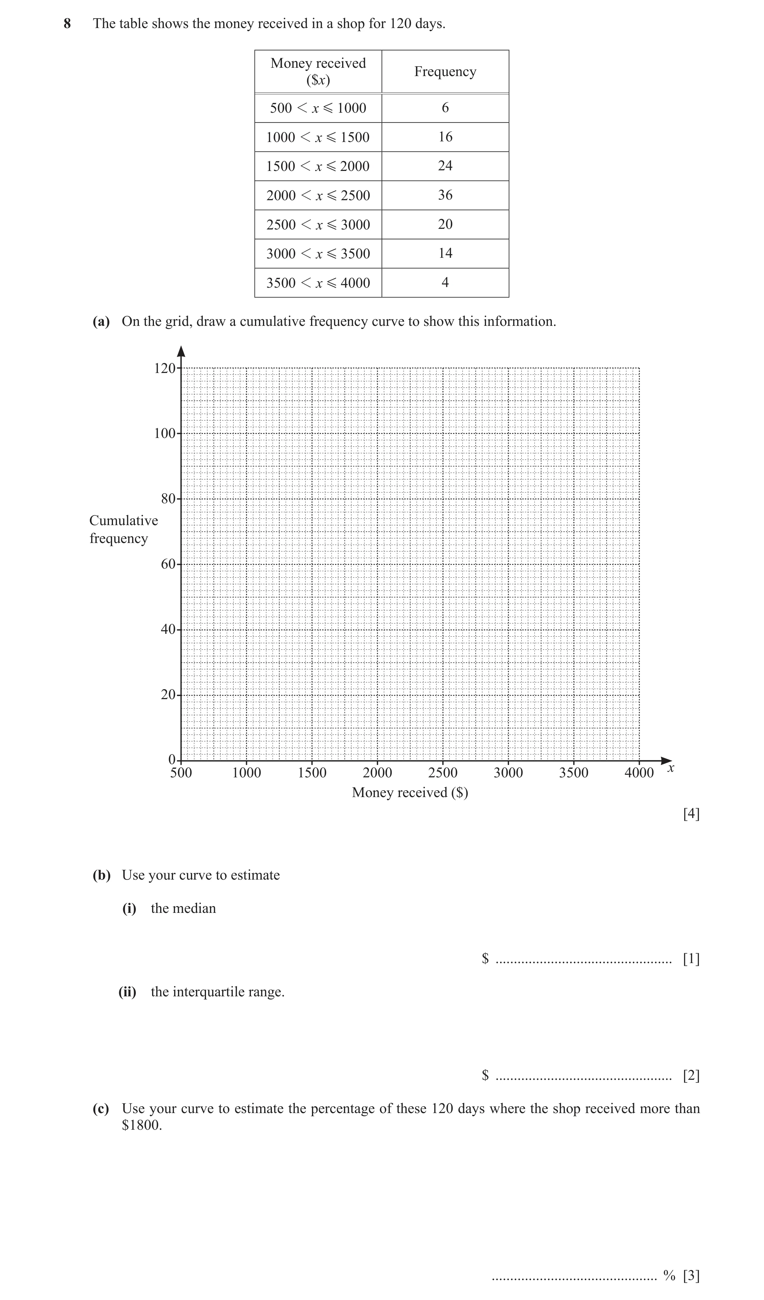
8 The table shows the money received in a shop for 120 days. Money received Frequency ($x) 500 1 x G 1000 6 1000 1 x G 1500 16 1500 1 x G 2000 24 2000 1 x G 2500 36 2500 1 x G 3000 20 3000 1 x G 3500 14 3500 1 x G 4000 4 (a) On the grid, draw a cumulative frequency curve to show this information. 120 100 80 Cumulative frequency 60 40 20 0 x 500 1000 1500 2000 2500 3000 3500 4000 Money received ($) [4] (b) Use your curve to estimate (i) the median $ … [1] (ii) the interquartile range. $ … [2] (c) Use your curve to estimate the percentage of these 120 days where the shop received more than $1800. … % [3]
10 marks
Mark scheme: 8(a) Correct graph through 7 points 4 B3 for graph through 5 correct points or B2 for graph through 3 correct points or for all correct heights translated to other point in interval or for correct points plotted not joined or B1 for 6, 22, 46, 82, 102, 116, 120 8(b)(i) 2100 to 2300 1 FT from increasing curve. 8(b)(ii) 950 to 1150 2 B1 for 1650 ⩽ [LQ] ⩽ 1750 or 2600 ⩽ [UQ] < 2750 8(c) 68.3 to 71.7 3 B1FT for 34 to 38 their M1 for (34to38)[100] 120 120 − their or (34to38)[100] 120
This question in 0607/42 Feb/March 2024
Q21 · The table shows the heights of 100 sunflower plants 0607/43 Oct/Nov 2024
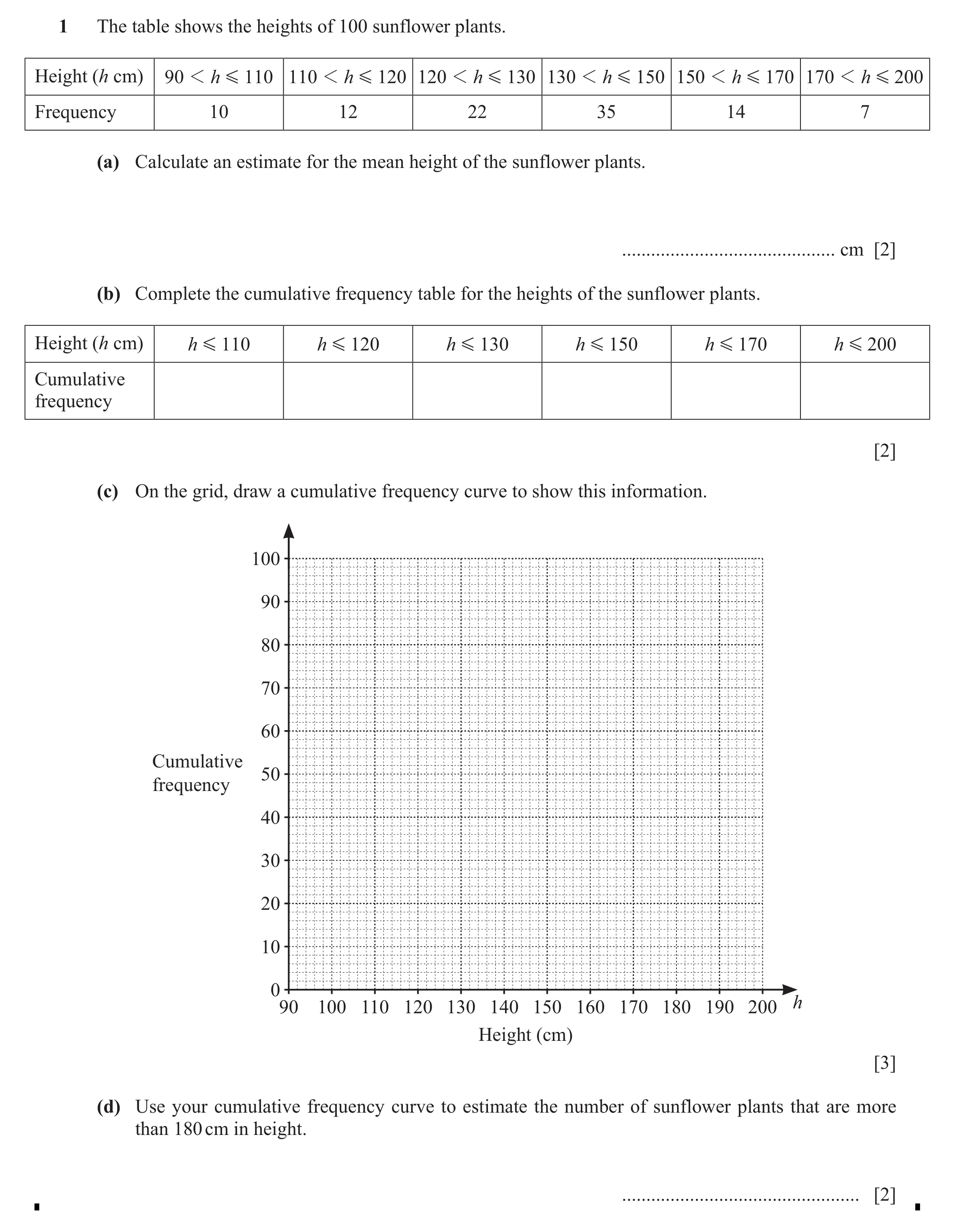
1 The table shows the heights of 100 sunflower plants. Height (h cm) 90 1 h G 11 0 110 1 h G 120 12 0 1 h G 130 130 1 h G 150 150 1 h G 170 170 1 h G 200 Frequency 10 12 22 35 14 7 (a) Calculate an estimate for the mean height of the sunflower plants. … cm [2] (b) Complete the cumulative frequency table for the heights of the sunflower plants. Height (h cm) h G 110 h G 120 h G 130 h G 150 h G 170 h G 200 Cumulative frequency [2] (c) On the grid, draw a cumulative frequency curve to show this information. 100 90 80 70 60 Cumulative 50 frequency 40 30 20 10 0 90 100 110 120 130 140 150 160 170 180 190 200 h Height (cm) [3] (d) Use your cumulative frequency curve to estimate the number of sunflower plants that are more than 180 cm in height. … [2]
9 marks
Mark scheme: Question Answer Marks Partial Marks 1(a) 136 or 135.65 or 135.7 2 M1 for midpoints soi 1(b) 10, 22, 44, 79, 93, 100 2 M1 for 4 correct 1(c) Correct cumulative frequency 3 FT their table with increasing values curve B1 for 6 points with correct heights B1 for 6 points with correct h values 1(d) 2, 3, 4 or 5 2 FT their increasing curve or polygon B1 for reading from their curve at 180 soi by 95 or 96 or 97 or 98
This question in 0607/43 Oct/Nov 2024
Q22 · The table shows some information about the heights, in cm, of 120 plants 0607/41 Oct/Nov 2025
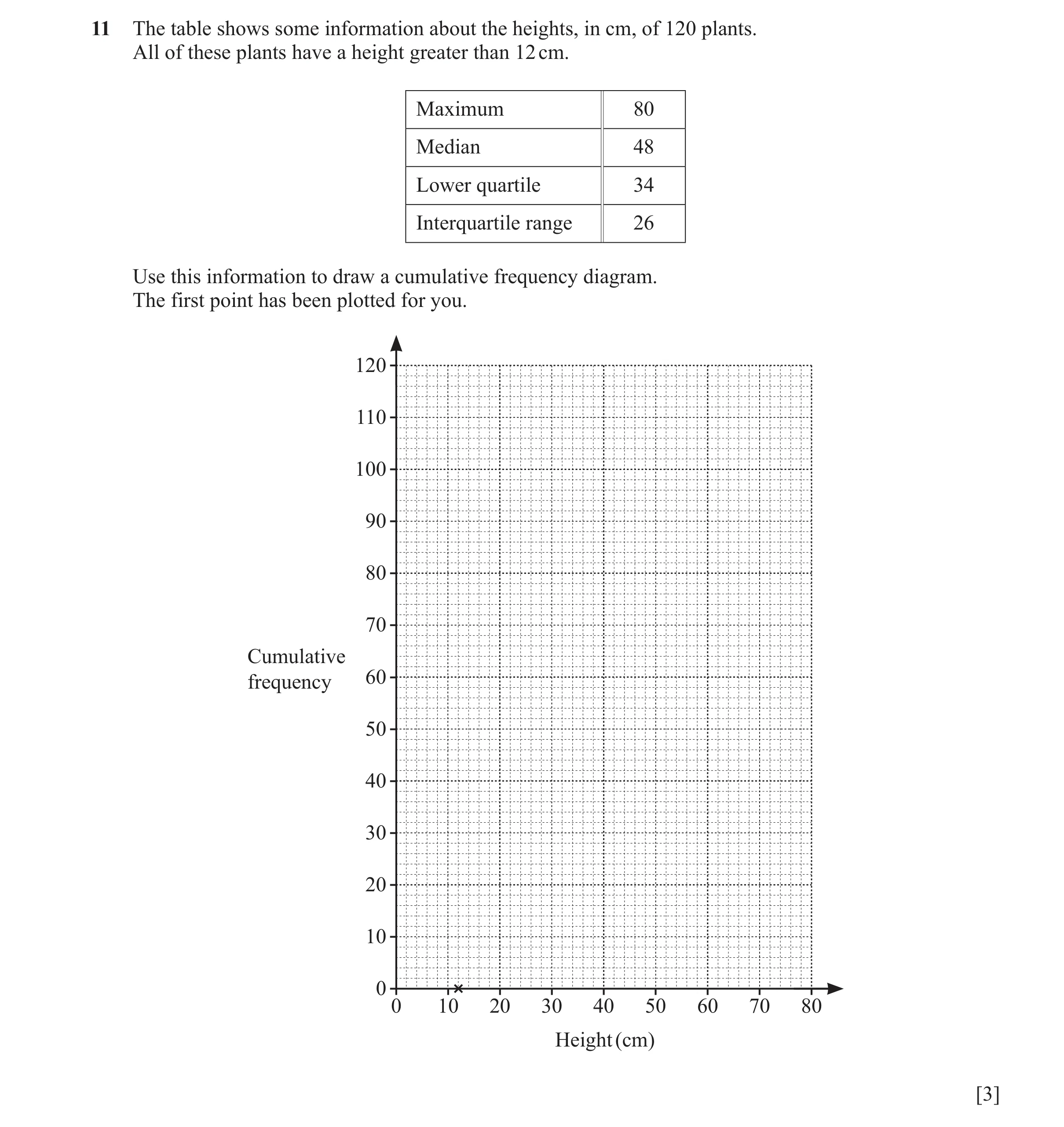
11 The table shows some information about the heights, in cm, of 120 plants. All of these plants have a height greater than 12 cm. Maximum 80 Median 48 Lower quartile 34 Interquartile range 26 Use this information to draw a cumulative frequency diagram. The first point has been plotted for you. 120 110 100 90 80 70 Cumulative frequency 60 50 40 30 20 10 0 0 10 20 30 40 50 60 70 80 Height (cm) [3]
3 marks
Mark scheme: 11 Correct diagram drawn through 5 3 B1 for points (80, 120) and (48, 60) correct points B1 for point (34, 30) B1 for point (60, 90) Maximum of 2 marks if diagram incorrect.
This question in 0607/41 Oct/Nov 2025
![Question 6: (a) These are Tom’s ten homework marks. 8 7 10 8 9 5 8 10 6 8 Find (i) the range, .................................................. [1] (i…](https://img.pastlit.com/crops/d96717a8-51ec-49c1-b3b9-d2d63513fcfe/q2.webp)
 28 / 33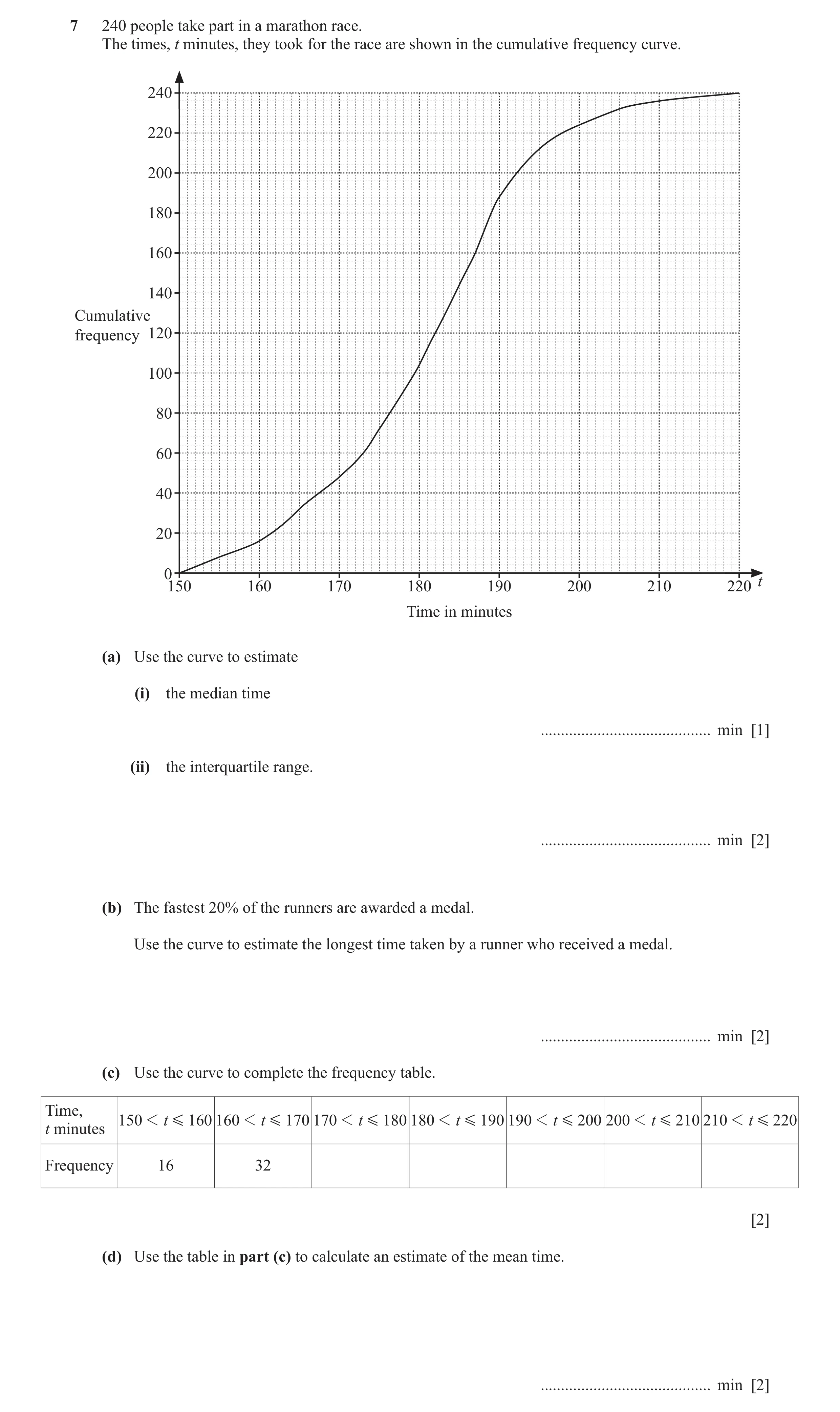
 32 / 33
 33 / 33
 12
12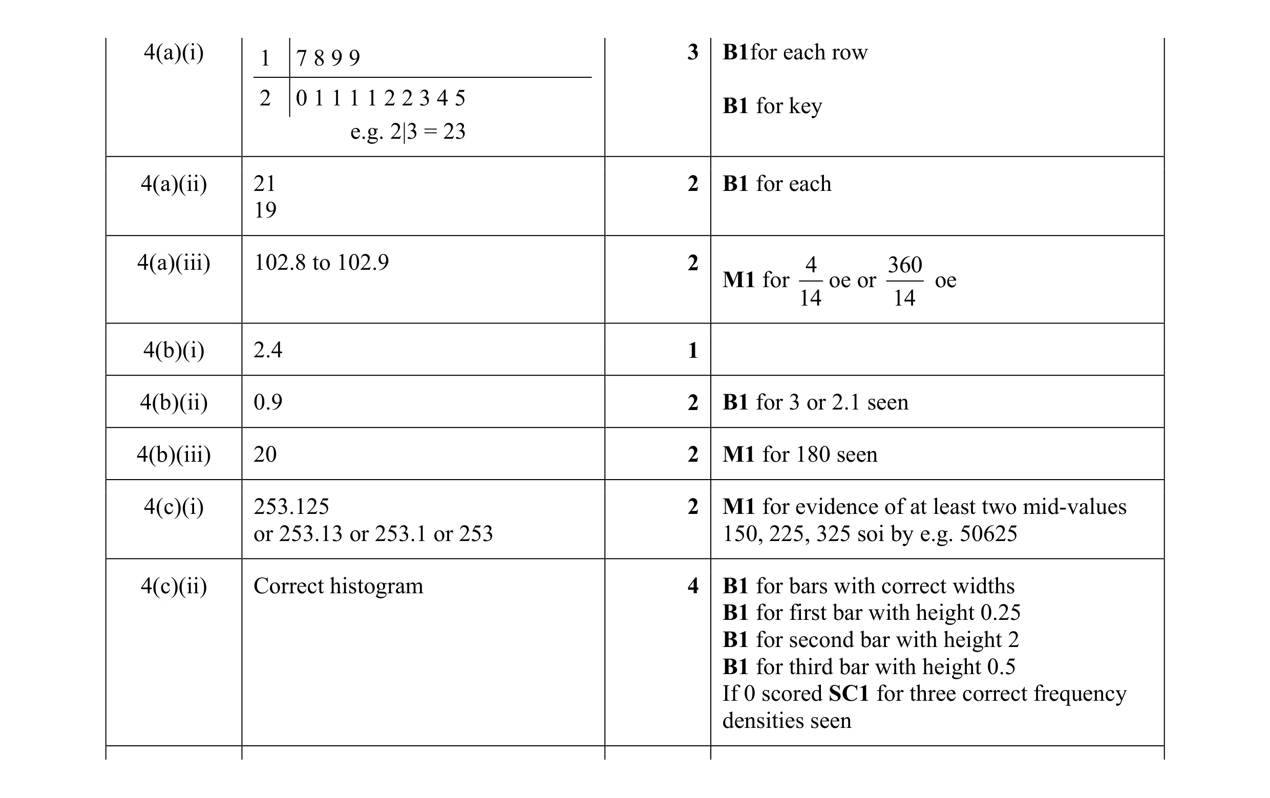 18
18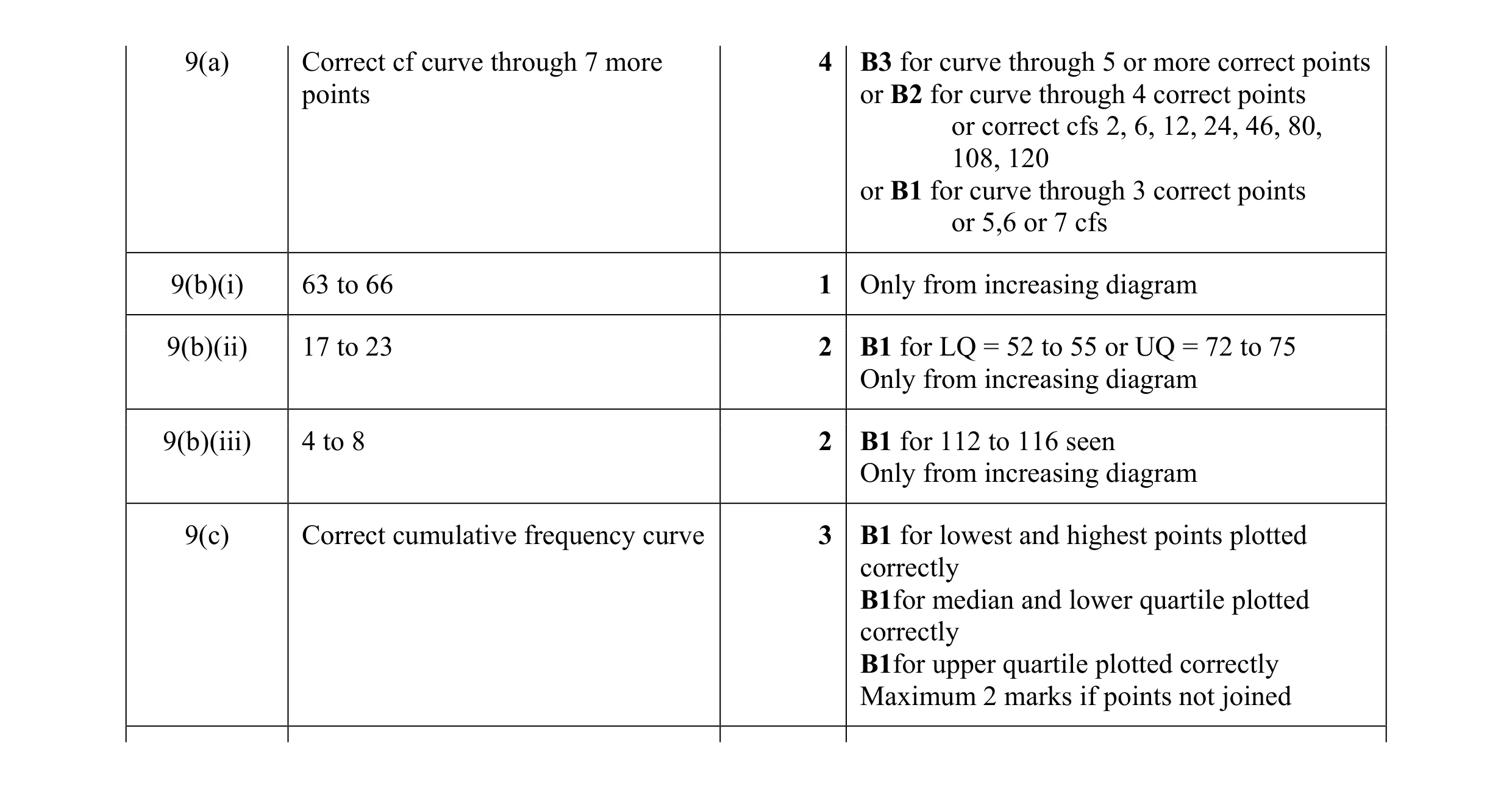 12
12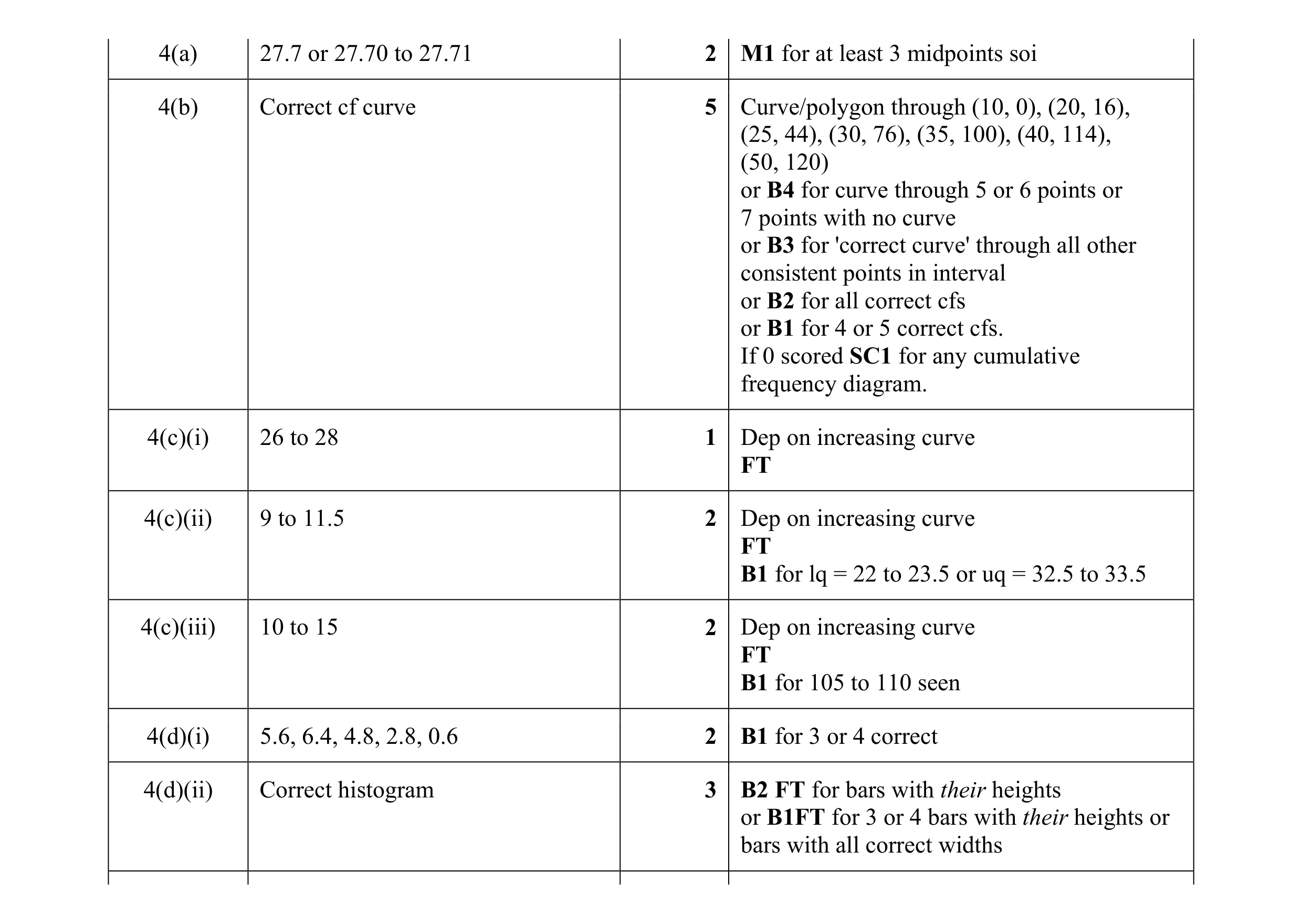 17
17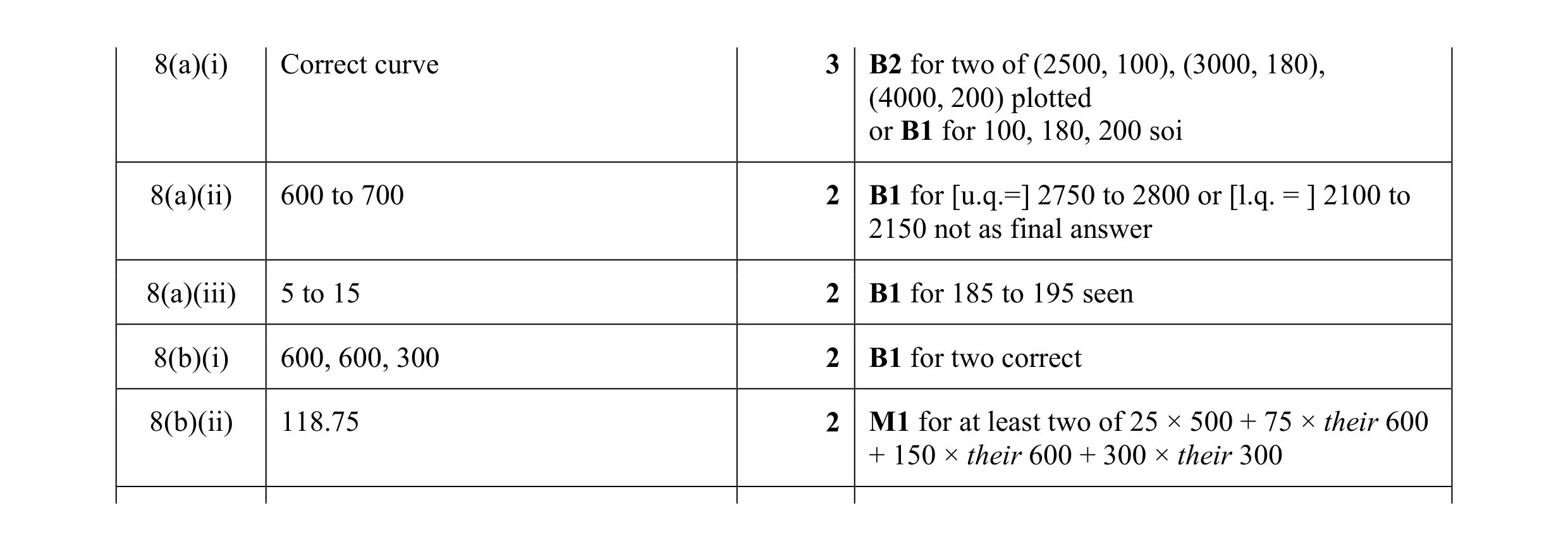 11
11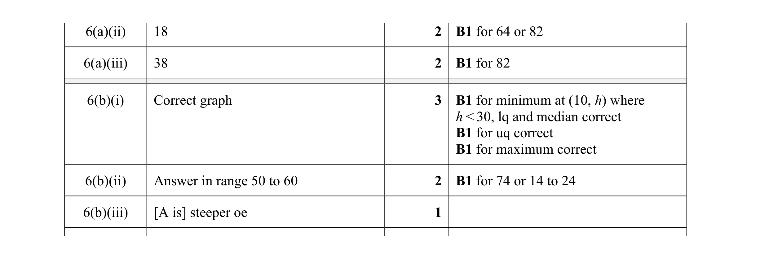 11
11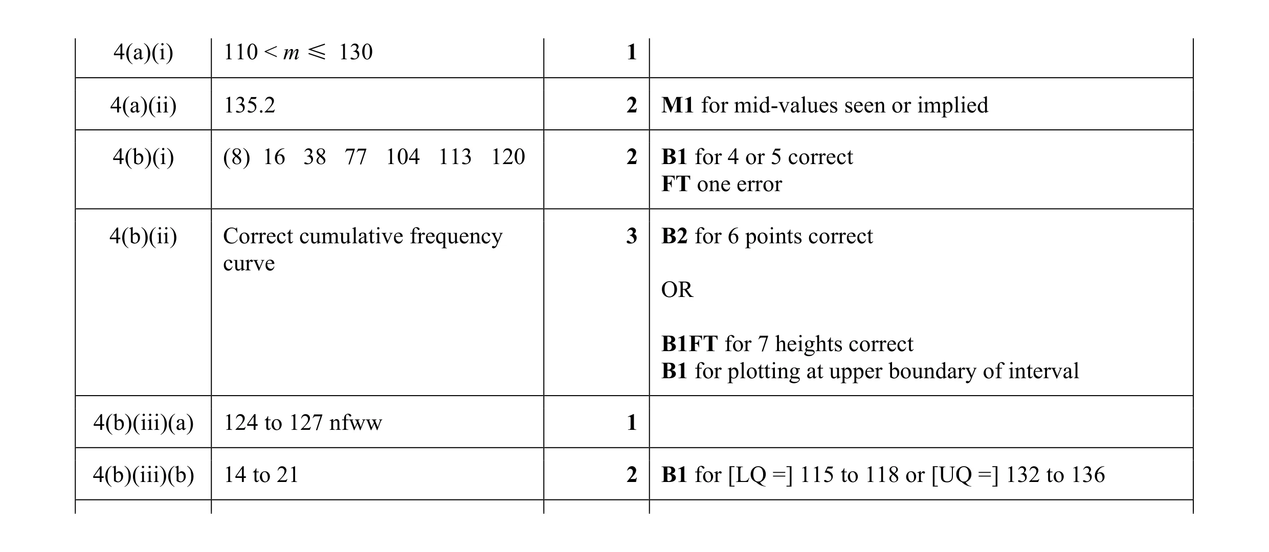 11
11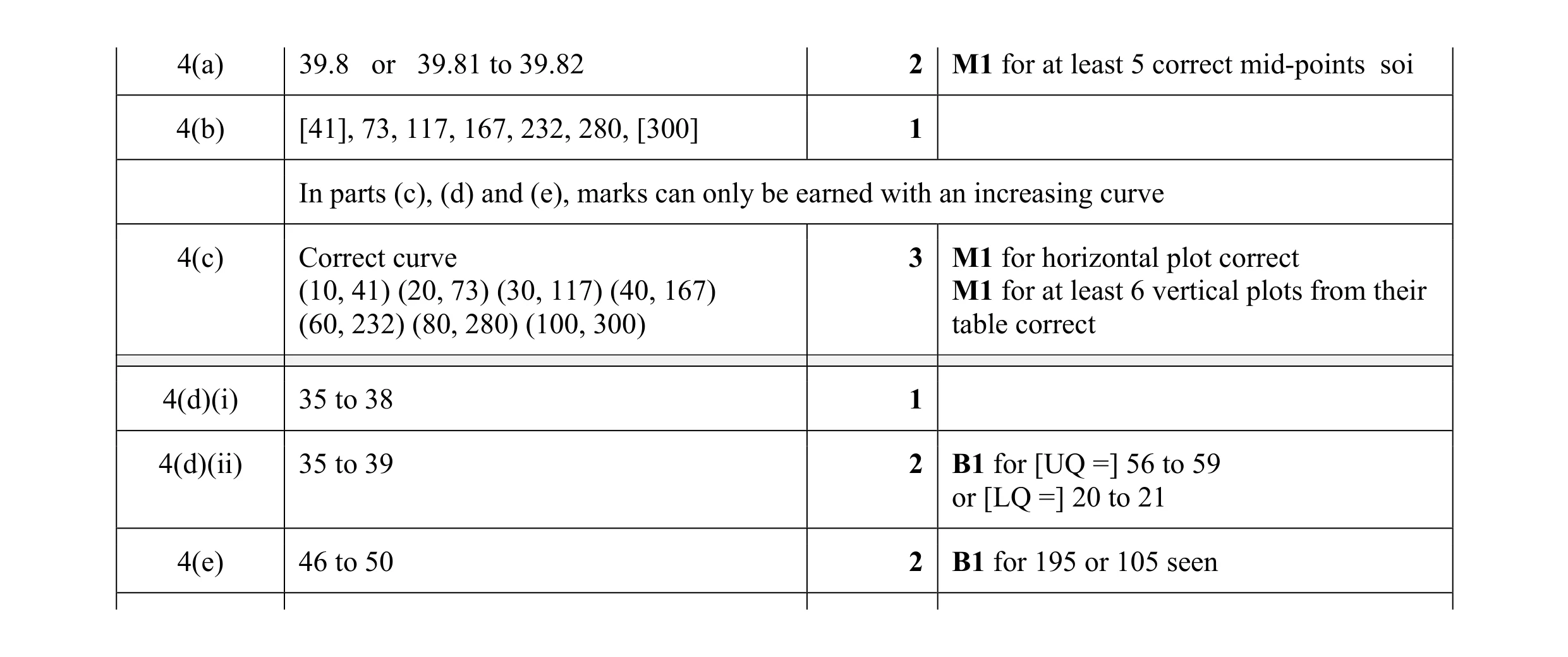 11
11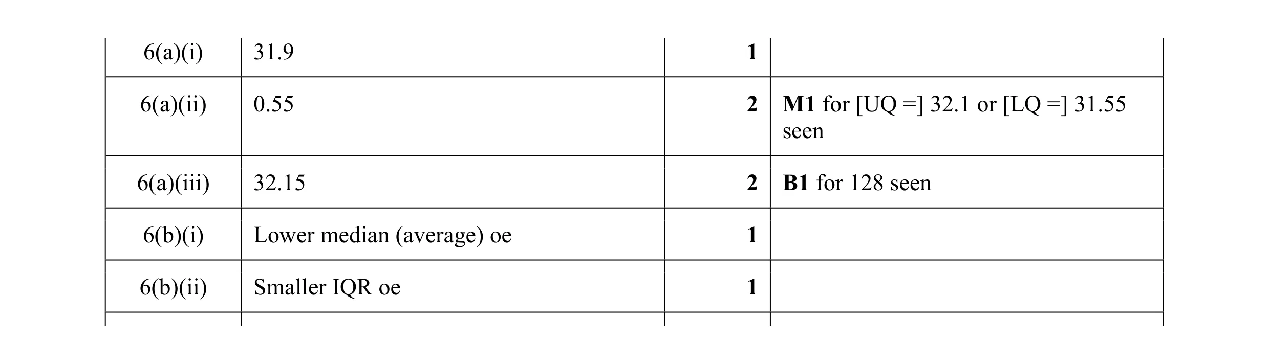 7
7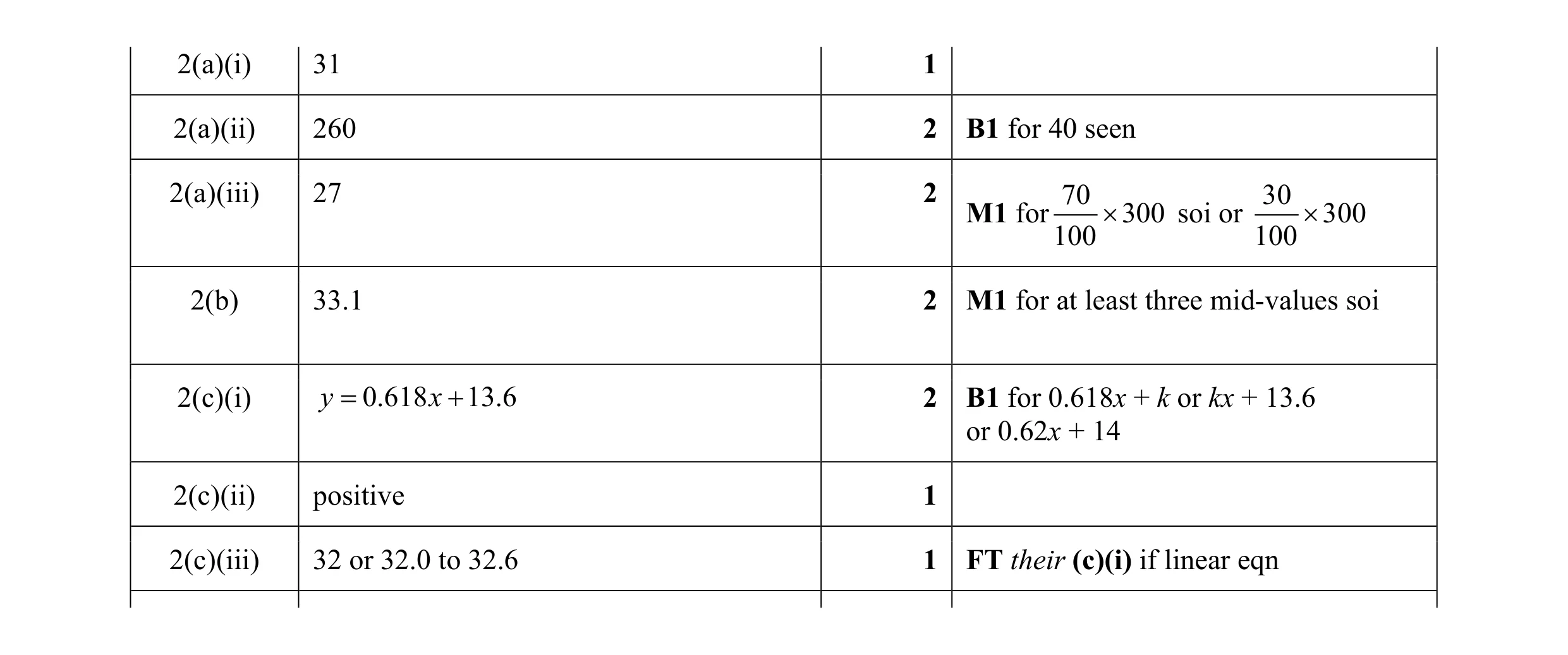 11
11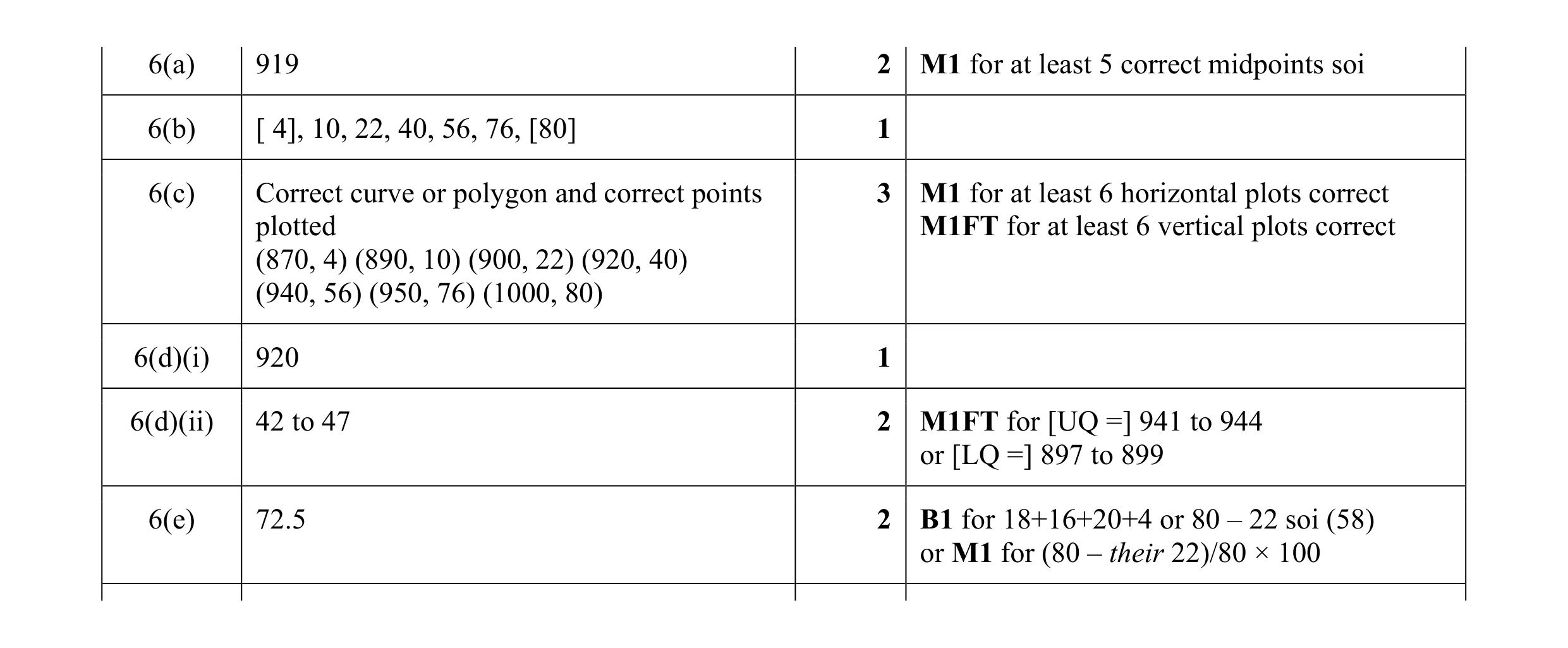 11
11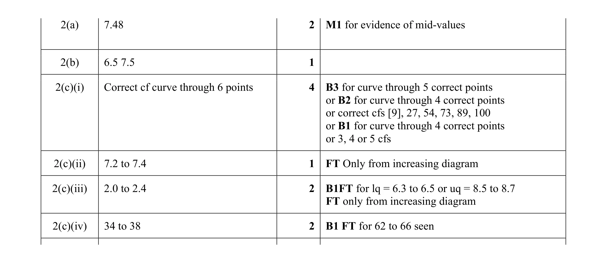 12
12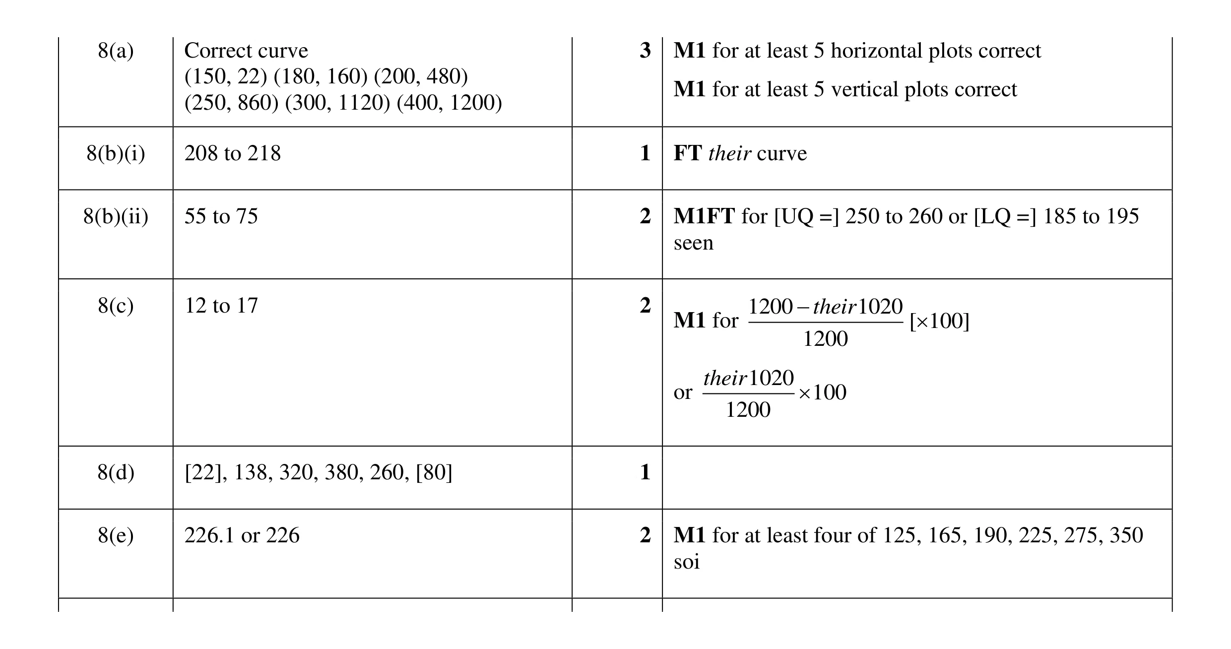 11
11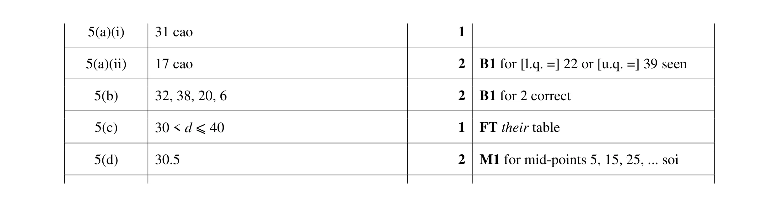 8
8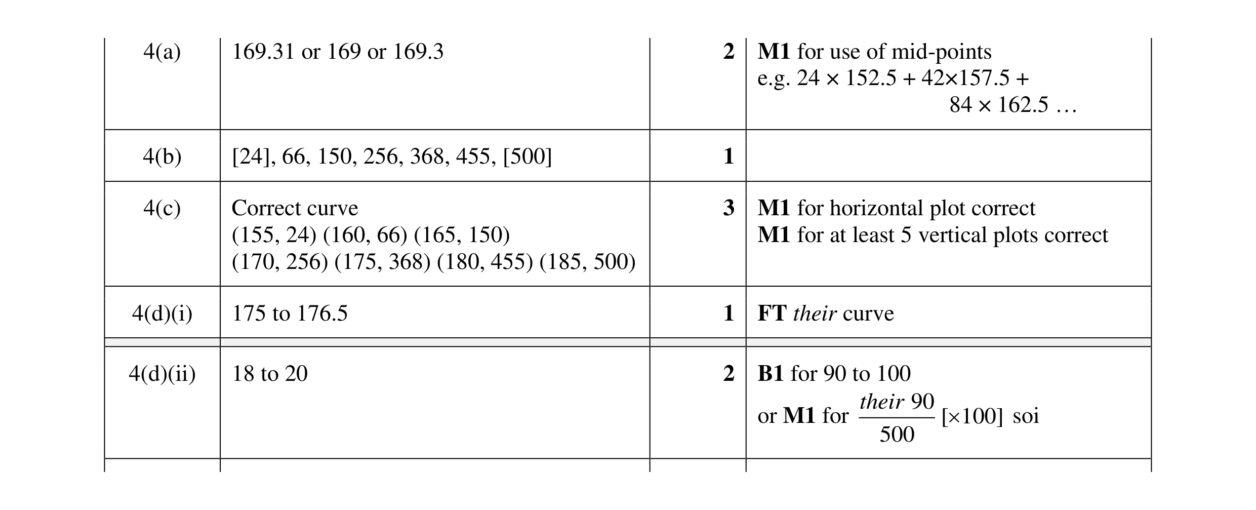 9
9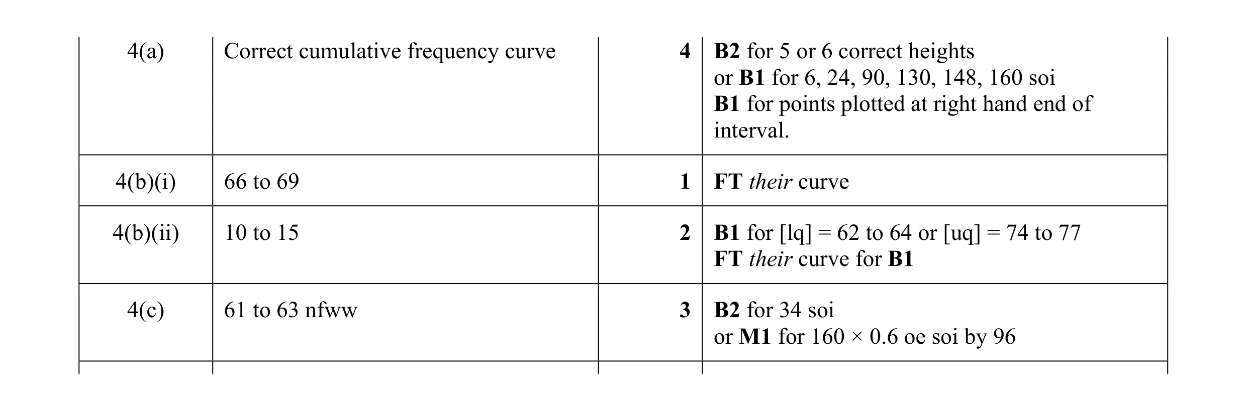 10
10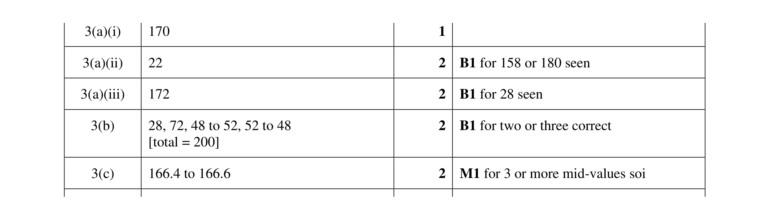 9
9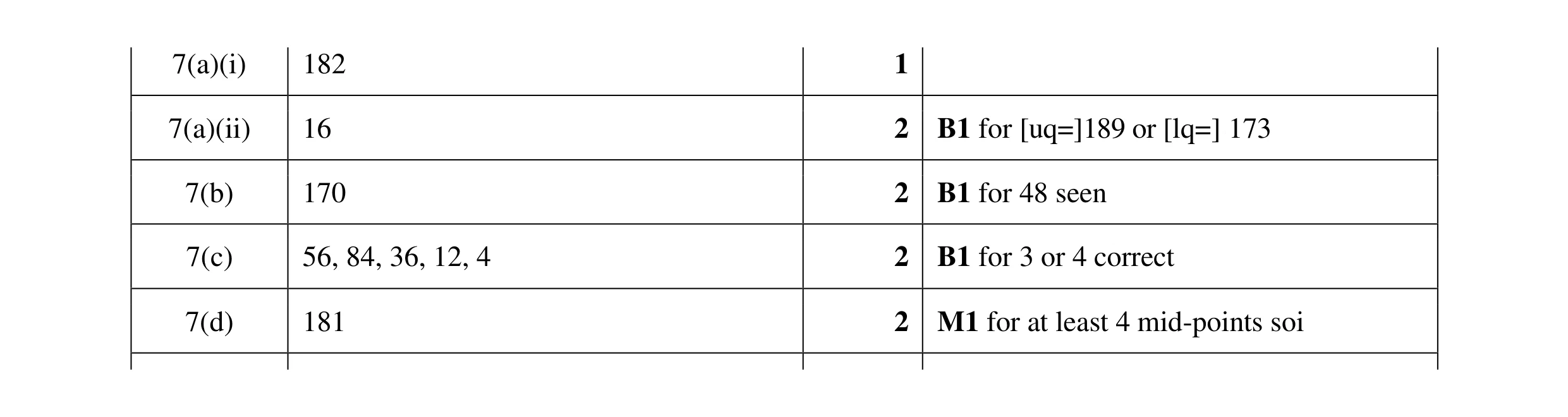 9
9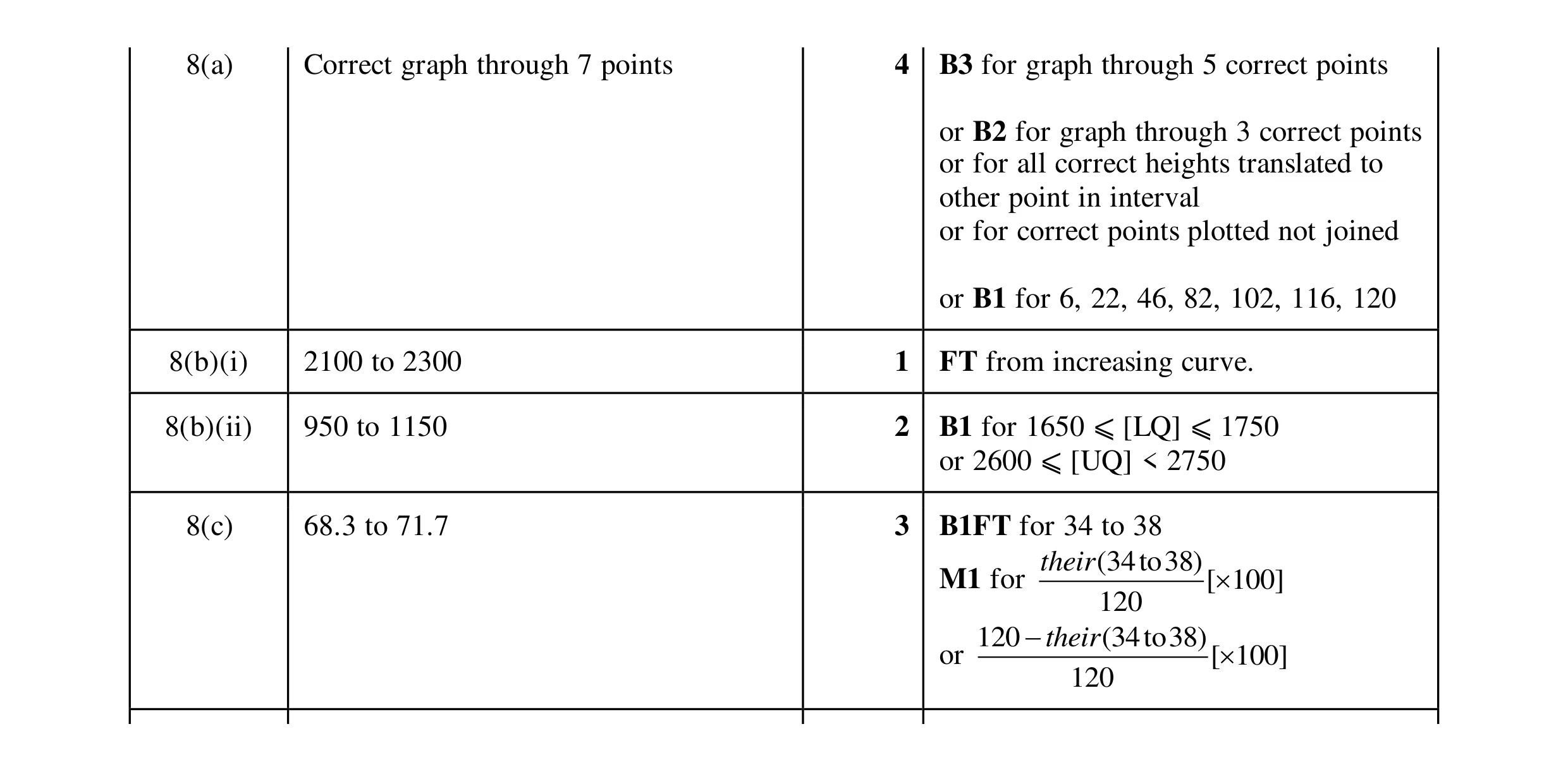 10
10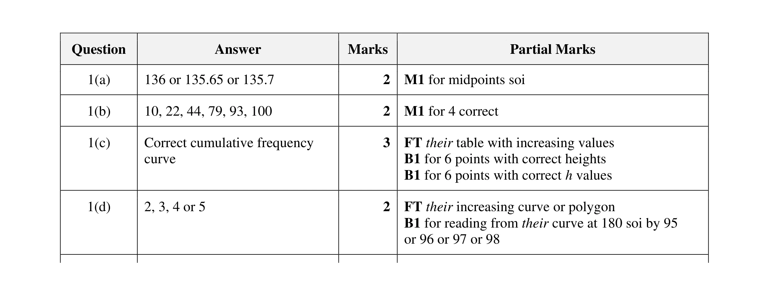 9
9 3
3