Questions as text
Q1 · Major avalanches can be regarded as randomly occurring events 9709/71 May/June 2009
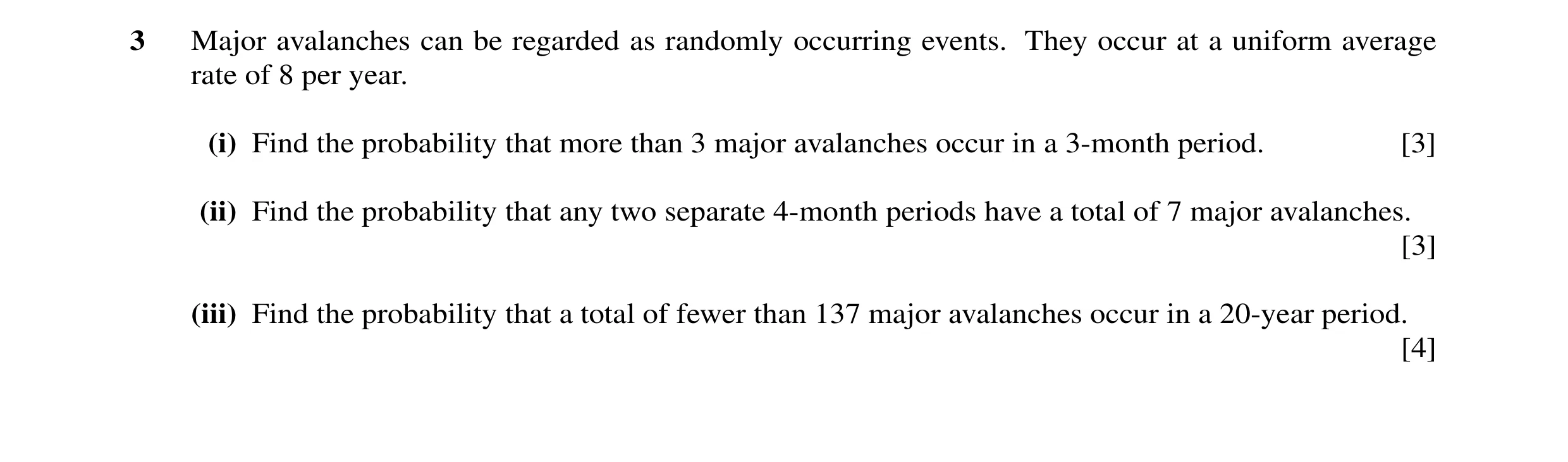
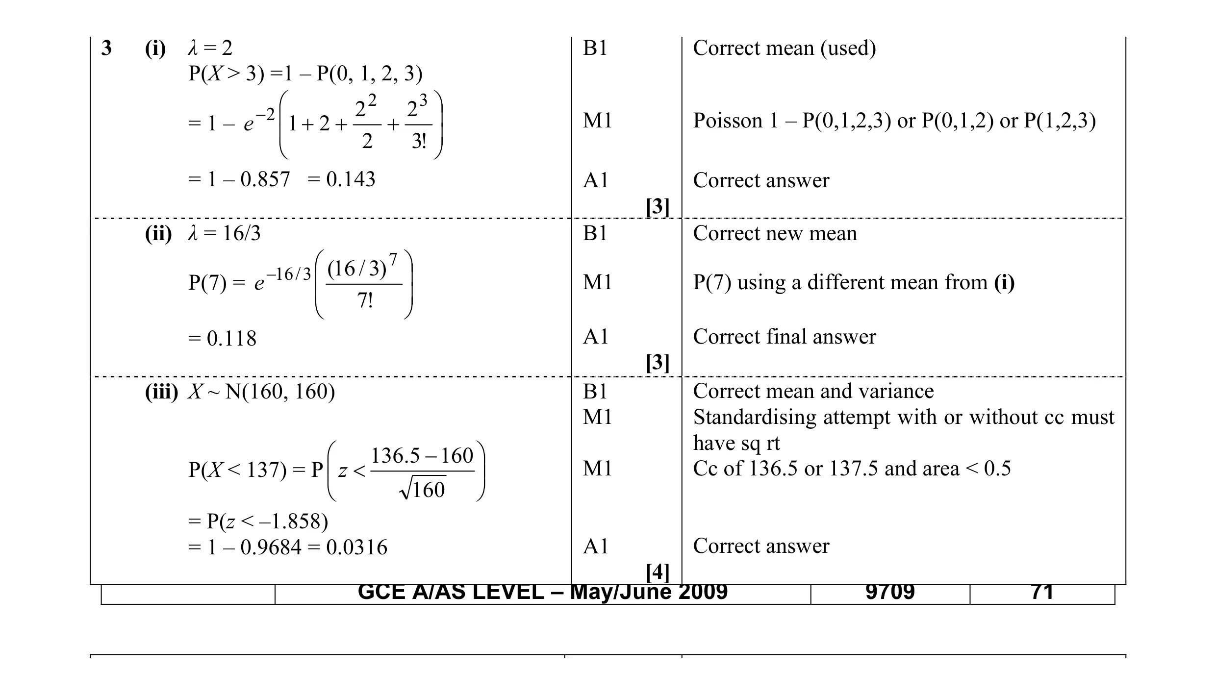
3 Major avalanches can be regarded as randomly occurring events. They occur at a uniform average rate of 8 per year. (i) Find the probability that more than 3 major avalanches occur in a 3-month period. [3] (ii) Find the probability that any two separate 4-month periods have a total of 7 major avalanches. [3] (iii) Find the probability that a total of fewer than 137 major avalanches occur in a 20-year period. [4]
10 marks
Mark scheme: 3 (i) λ = 2 B1 Correct mean (used) P(X > 3) =1 – P(0, 1, 2, 3) 2 3 2 2 − 2 M1 Poisson 1 – P(0,1,2,3) or P(0,1,2) or P(1,2,3) 1 + 2 + + = 1 – e 2 !3 = 1 – 0.857 = 0.143 A1 Correct answer [3] (ii) λ = 16/3 B1 Correct new mean 7 (16 / 3) −16 / 3 M1 P(7) using a different mean from (i) P(7) = e !7 = 0.118 A1 Correct final answer [3] (iii) X ~ N(160, 160) B1 Correct mean and variance M1 Standardising attempt with or without cc must have sq rt 1365. − 160 P(X < 137) = P z < M1 Cc of 136.5 or 137.5 and area < 0.5 160 = P(z < –1.858) = 1 – 0.9684 = 0.0316 A1 Correct answer [4] GCE A/AS LEVEL – May/June 2009 9709 71
This question in 9709/71 May/June 2009
Q2 · A computer user finds that unwanted emails arrive randomly at a uniform average rate of… 9709/72 Oct/Nov 2009
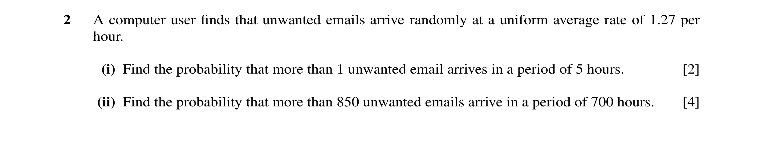
2 A computer user finds that unwanted emails arrive randomly at a uniform average rate of 1.27 per hour. (i) Find the probability that more than 1 unwanted email arrives in a period of 5 hours. [2] (ii) Find the probability that more than 850 unwanted emails arrive in a period of 700 hours. [4]
6 marks
Mark scheme: 2 (i) λ = 6.35 M1 Attempt at Poisson, 1 – (P(0) + P(1)) with P(> 1) = 1 – e–6.35 (1 + 6.35) their λ. Accept 1 – P(0). = 0.987 A1 Correct answer. [2] (ii) λ = 889 B1 Correct mean 8505. − 889 P(> 850) = 1 – Φ M1* Standardising, with or without continuity 889 correction using their N(889, 889). Condone sd/var mixes. = Φ(1.29) or Φ(1.31) with no cc M1*dep Correct area (> 0.5) with or without cc = 0.902 A1 Correct answer [4]
This question in 9709/72 Oct/Nov 2009
Q3 · People arrive randomly and independently at a supermarket checkout at an average rate of… 9709/71 Oct/Nov 2010
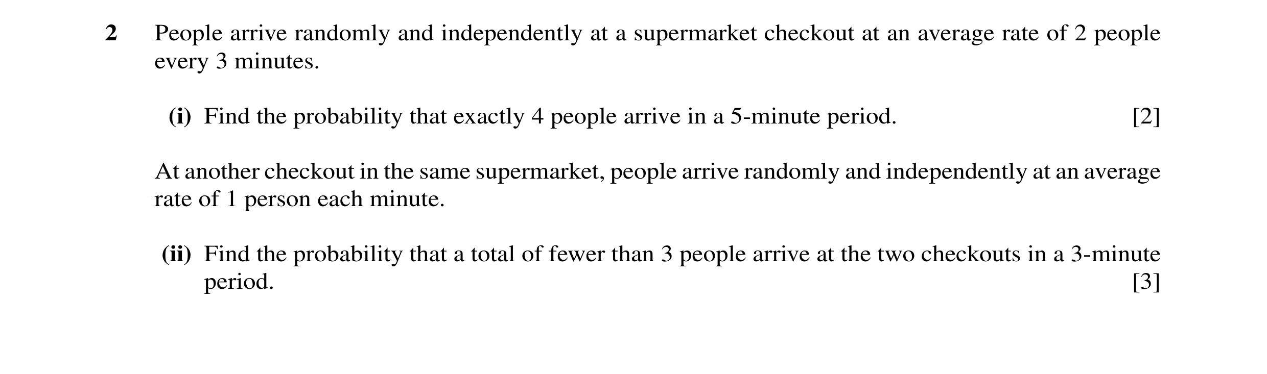
2 People arrive randomly and independently at a supermarket checkout at an average rate of 2 people every 3 minutes. (i) Find the probability that exactly 4 people arrive in a 5-minute period. [2] At another checkout in the same supermarket, people arrive randomly and independently at an average rate of 1 person each minute. (ii) Find the probability that a total of fewer than 3 people arrive at the two checkouts in a 3-minute period. [3]
5 marks
Mark scheme: − 103 ( 103 ) 42 (i) e × 4! M1 Allow incorrect λ = 0.184 or 0.183 A1 [2] (ii) λ = 5 B1 e −5 1( + 5 + 522 ) M1 Allow incorrect λ. Allow one end error = 0.125 (3 sfs) A1 [3] OR Combination method scores B1, identifying all 6 possible combinations M1, multiply each combination and add (must use at least 5 combinations) A1
This question in 9709/71 Oct/Nov 2010
Q4 · People arrive randomly and independently at a supermarket checkout at an average rate of… 9709/72 Oct/Nov 2010
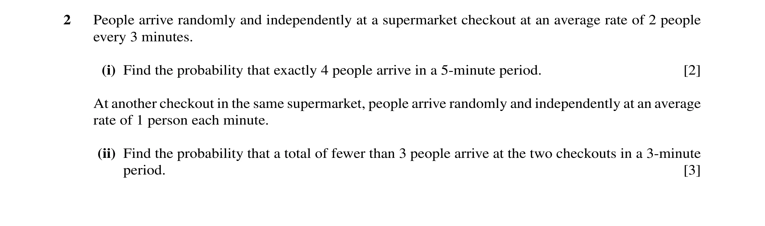
2 People arrive randomly and independently at a supermarket checkout at an average rate of 2 people every 3 minutes. (i) Find the probability that exactly 4 people arrive in a 5-minute period. [2] At another checkout in the same supermarket, people arrive randomly and independently at an average rate of 1 person each minute. (ii) Find the probability that a total of fewer than 3 people arrive at the two checkouts in a 3-minute period. [3]
5 marks
Mark scheme: − 103 ( 103 ) 42 (i) e × 4! M1 Allow incorrect λ = 0.184 or 0.183 A1 [2] (ii) λ = 5 B1 e −5 1( + 5 + 522 ) M1 Allow incorrect λ. Allow one end error = 0.125 (3 sfs) A1 [3] OR Combination method scores B1, identifying all 6 possible combinations M1, multiply each combination and add (must use at least 5 combinations) A1
This question in 9709/72 Oct/Nov 2010
Q5 · In the past, the number of house sales completed per week by a building company has been… 9709/73 Oct/Nov 2010
7 In the past, the number of house sales completed per week by a building company has been modelled by a random variable which has the distribution Po(0.8). Following a publicity campaign, the builders hope that the mean number of sales per week will increase. In order to test at the 5% significance level whether this is the case, the total number of sales during the first 3 weeks after the campaign is noted. It is assumed that a Poisson model is still appropriate. (i) Given that the total number of sales during the 3 weeks is 5, carry out the test. [6] (ii) During the following 3 weeks the same test is carried out again, using the same significance level. Find the probability of a Type I error. [3] (iii) Explain what is meant by a Type I error in this context. [1] (iv) State what further information would be required in order to find the probability of a Type II error. [1]
11 marks
Mark scheme: 7 (i) H0: mean no. sales = 2.4 B1 Or “= 0.8 per week” H1: mean no. sales > 2.4 Accept λ, not µ. P(X > 5) M1* Attempted with or without “1–“. 4.2 2 4.2 3 4.2 4 Allow one end error. = 1 – e-2.4(1 + 2.4 + + + !2 !3 !4 (= 1 – 0.9041) A1 Allow incorrect λ in otherwise correct expression. = 0.0959 A1 Comp with 0.05 M1* Indep M. (Allow recovery of above 3 marks at this point if comparison with 0.95 done.) No evidence to believe mean sales incr A1ft dep [6] Conclusion, no contradictions. 4.2 5 SC: e-2.4 × = 0.0602 > 0.05: !5 max B1M0A0A0M1A0 (ii) Need 1st x such that P(X > x) < 0.05 M1* Attempt sum of at least 3 relevant Poisson terms, with comparison with 0.05 (can be implied). Can be implied, e.g. by P(X < 5) = 0.9643 identified. 4.2 5 P(X > 6) = 1 – e–2.4(1 + 2.4 + . . . + ) M1*dep !5 (= 1 – 0.9643) = 0.0357 A1 [3] (iii) Mean sales still 0.8 per week, but > 6 sales Conclude mean sales have increased in 3 weeks, so reject 0.8. B1 [1] when not true (iv) Value of true (new, changed) mean oe B1 [1]
This question in 9709/73 Oct/Nov 2010
Q6 · The number of injuries per month at a certain factory has a Poisson distribution 9709/71 May/June 2011
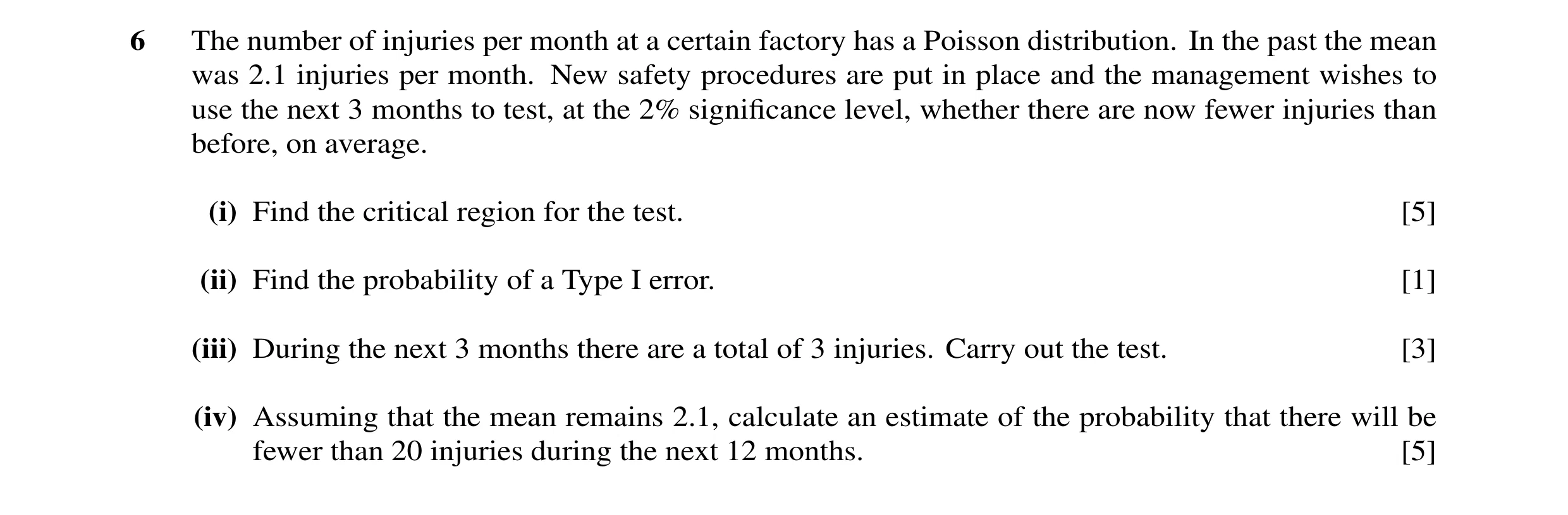
6 The number of injuries per month at a certain factory has a Poisson distribution. In the past the mean was 2.1 injuries per month. New safety procedures are put in place and the management wishes to use the next 3 months to test, at the 2% significance level, whether there are now fewer injuries than before, on average. (i) Find the critical region for the test. [5] (ii) Find the probability of a Type I error. [1] (iii) During the next 3 months there are a total of 3 injuries. Carry out the test. [3] (iv) Assuming that the mean remains 2.1, calculate an estimate of the probability that there will be fewer than 20 injuries during the next 12 months. [5]
14 marks
Mark scheme: 6 (i) mean = 6.3 B1 B1 for 6.3 P(X < 1) = e–6.3(1 + 6.3) = 0.0134 M1 Allow incorrect λ in both probs 3.6 2 P(X < 2) = e–6.3(1 + 6.3 + ) = 0.0498 M1A1 2 CR is X < 1 A1 A1 for both values [5] (ii) P(Type I error) = P(X < 1) = 0.0134 B1 [1] (iii) H0: λ = 6.3 H1: λ < 6.3 B1 Can be scored in (i). Accept λ = 2.1(per month) 3 not in CR M1 or P(X < 3) = 0.126 > 0.02 No evidence mean no. of injuries has decreased A1 Correct conclusion [3] (iv) N(25.2, 25.2) B2 B1 for N & µ = 25.2. B1 for σ2 = 25.2 May be implied 195. − 252. (= –1.135) M1 Allow with wrong or no cc or no √ 252. Φ(“–1.135”) = 1 – Φ(“1.135”) M1 Correct area = 0.128 (3 sfs) A1 [5]
This question in 9709/71 May/June 2011
Q7 · The random variable X has the distribution Po(1.3) 9709/71 Oct/Nov 2011
1 The random variable X has the distribution Po(1.3). The random variable Y is defined by Y = 2X. (i) Find the mean and variance of Y. [3] (ii) Give a reason why the variable Y does not have a Poisson distribution. [1]
4 marks
Mark scheme: 1 (i) Mean = 2.6 B1 Var = 4 × 1.3 M1 M1 for either 4 ×, or for Var(X ) = 1.3 implied = 5.2 A1 [3] (ii) Var ≠ mean B1 X and X are not independent oe or 2X does not take all integer values [1] 1
This question in 9709/71 Oct/Nov 2011
Q8 · Customers arrive at an enquiry desk at a constant average rate of 1 every 5 minutes 9709/71 Oct/Nov 2011
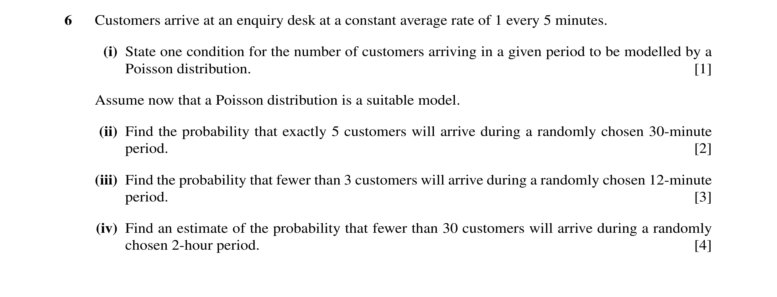
6 Customers arrive at an enquiry desk at a constant average rate of 1 every 5 minutes. (i) State one condition for the number of customers arriving in a given period to be modelled by a Poisson distribution. [1] Assume now that a Poisson distribution is a suitable model. (ii) Find the probability that exactly 5 customers will arrive during a randomly chosen 30-minute period. [2] (iii) Find the probability that fewer than 3 customers will arrive during a randomly chosen 12-minute period. [3] (iv) Find an estimate of the probability that fewer than 30 customers will arrive during a randomly chosen 2-hour period. [4]
10 marks
Mark scheme: 6 (i) Customers arrive independently or randomly B1 [1] In context. Allow “singly” − 6 65 (ii) e × M1 Poisson P(5), allow any mean !5 = 0.161 (3 sfs) A1 [2] (iii) λ = 2.4 B1 − 2 4.2 2 e 1 + 4.2 + M1 Poisson P(0, 1, 2), allow their mean !2 allow one end error = 0.570 (3 sfs) A1 [3] (iv) N(24, 24) B1 Stated or implied 295 − 24 (= 1.123) M1 Allow with wrong or no cc and/or no √ 24 Correct area Φ (“1.123”) M1 = 0.869 (3 sfs) A1 [4] GCE AS/A LEVEL – October/November 2011 9709 71
This question in 9709/71 Oct/Nov 2011
Q9 · The random variable X has the distribution Po(1.3) 9709/72 Oct/Nov 2011
1 The random variable X has the distribution Po(1.3). The random variable Y is defined by Y = 2X. (i) Find the mean and variance of Y. [3] (ii) Give a reason why the variable Y does not have a Poisson distribution. [1]
4 marks
Mark scheme: 1 (i) Mean = 2.6 B1 Var = 4 × 1.3 M1 M1 for either 4 ×, or for Var(X ) = 1.3 implied = 5.2 A1 [3] (ii) Var ≠ mean B1 X and X are not independent oe or 2X does not take all integer values [1] 1
This question in 9709/72 Oct/Nov 2011
Q10 · Customers arrive at an enquiry desk at a constant average rate of 1 every 5 minutes 9709/72 Oct/Nov 2011
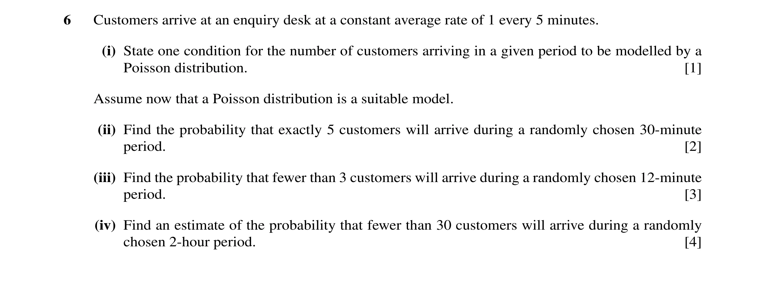
6 Customers arrive at an enquiry desk at a constant average rate of 1 every 5 minutes. (i) State one condition for the number of customers arriving in a given period to be modelled by a Poisson distribution. [1] Assume now that a Poisson distribution is a suitable model. (ii) Find the probability that exactly 5 customers will arrive during a randomly chosen 30-minute period. [2] (iii) Find the probability that fewer than 3 customers will arrive during a randomly chosen 12-minute period. [3] (iv) Find an estimate of the probability that fewer than 30 customers will arrive during a randomly chosen 2-hour period. [4]
10 marks
Mark scheme: 6 (i) Customers arrive independently or randomly B1 [1] In context. Allow “singly” − 6 65 (ii) e × M1 Poisson P(5), allow any mean !5 = 0.161 (3 sfs) A1 [2] (iii) λ = 2.4 B1 − 2 4.2 2 e 1 + 4.2 + M1 Poisson P(0, 1, 2), allow their mean !2 allow one end error = 0.570 (3 sfs) A1 [3] (iv) N(24, 24) B1 Stated or implied 295 − 24 (= 1.123) M1 Allow with wrong or no cc and/or no √ 24 Correct area Φ (“1.123”) M1 = 0.869 (3 sfs) A1 [4] GCE AS/A LEVEL – October/November 2011 9709 72
This question in 9709/72 Oct/Nov 2011
Q11 · The numbers of men and women who visit a clinic each hour are independent Poisson… 9709/73 Oct/Nov 2011
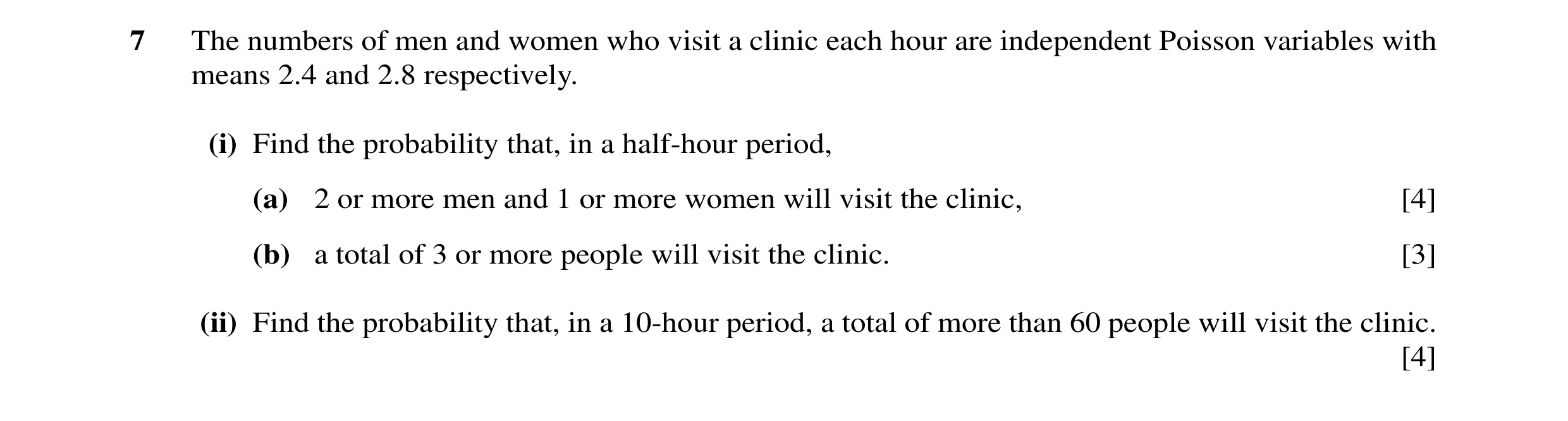
7 The numbers of men and women who visit a clinic each hour are independent Poisson variables with means 2.4 and 2.8 respectively. (i) Find the probability that, in a half-hour period, (a) 2 or more men and 1 or more women will visit the clinic, [4] (b) a total of 3 or more people will visit the clinic. [3] (ii) Find the probability that, in a 10-hour period, a total of more than 60 people will visit the clinic. [4]
11 marks
Mark scheme: 7 (i) (a) 1 – e–1.2(1 + 1.2) (= 0.3374) M1 M1 for Poisson either P(0 or 1) or P(0) 1 – e–1.4 (= 0.7534) A1 with λ = 1.2 or 2.4 or 1.4 or 2.8, accept one end error Both expressions fully correct (1 – e–1.2(1 + 1.2)) × (1 – e–1.4) M1 Their Poisson P(0 or 1) × P(0) = 0.254 (3 sfs) A1 [4] (i) (b) λ = 2.6 seen B1 1 – e–2.6(1 + 2.6 + 2.62 ÷ 2) M1 Poisson 1 – P(0, 1, 2), allow 1 – P(0, 1, 2, 3), with attempt at combined λ for M and W. Accept combination method: at least 4 correct terms and “1 –” M1; all terms correct B1 = 0.482 (3 sfs) A1 [3] GCE AS/A LEVEL – October/November 2011 9709 73 (ii) N(52, 52) B1 Seen or implied 605. − 52 M1 Standardising with N(λ, λ) with (= 1.179) 52 λ = 10 × 5.2 or 10 × 2.6 Allow with wrong or no cc or no √ 1 – Φ(“1.179”) M1 Their correct area (= 1 – 0.8808) = 0.119 (3 sfs) A1 [4]
This question in 9709/73 Oct/Nov 2011
Q12 · A random variable X has the distribution Po(3.2) 9709/71 May/June 2012
5 A random variable X has the distribution Po(3.2). (i) A random value of X is found. (a) Find P(X ≥3). [2] (b) Find the probability that X = 3 given that X ≥3. [3] (ii) Random samples of 120 values of X are taken. (a) Describe fully the distribution of the sample mean. [2] (b) Find the probability that the mean of a random sample of size 120 is less than 3.3. [3]
10 marks
Mark scheme: 5 (i) (a) 2.3 2 M1 Allow one end error P(X > 3) = 1 – e–3.2 (1 + 3.2 + 2! ) = 0.62(0) (3 sf) A1 [2] 3 2.3 (b) P(X = 3) = e −2.3 (= 0.22262) M1 May be implied 3 P ( X = 3∩ X ≥ 3) P ( X = 3) = P ( X ≥ 3) P ( X ≥ 3) .0'22262 ' = .0'62010 ' M1 Their P ( X = 3) Their P ( X ≥ 3) = 0.359 (3 sf) A1 [3] (ii) (a) (Approx) normal with mean 3.2 B1 2.3 or variance = 120 75 2 or 0.0267 B1 or sd = 1202.3 or 0.163 (3 sfs) oe (3 sfs) oe [2] (b) 3.3 − 2.3 (= 0.612) M1 Allow with cc attempted 2.3 120 Φ (“0.612”) M1 = 0.730 (3 sfs) A1 Accept 0.73 [3]
This question in 9709/71 May/June 2012
Q13 · At work Jerry receives emails randomly at a constant average rate of 15 emails per hour 9709/71 May/June 2012
7 At work Jerry receives emails randomly at a constant average rate of 15 emails per hour. (i) Find the probability that Jerry receives more than 2 emails during a 20-minute period at work. [3] (ii) Jerry’s working day is 8 hours long. Find the probability that Jerry receives fewer than 110 emails per day on each of 2 working days. [4] (iii) At work Jerry also receives texts randomly and independently at a constant average rate of 1 text every 10 minutes. Find the probability that the total number of emails and texts that Jerry receives during a 5-minute period at work is more than 2 and less than 6. [4]
11 marks
Mark scheme: 7 (i) λ = 5 B1 52 1 – e–5(1 + 5 + !2 ) M1 Any λ. Allow one end error = 0.875 A1 [3] (ii) X ~ N(120, 120) B1 May be implied 1095. −120 (= –0.9585) M1 Allow with wrong or no cc or no √ 120 1 – Φ(“0.9585”) M1 (= 1 – 0.8312) “0.1688”2 = 0.0285 to 0.0286 A1 [4] (iii) λ = 15 × 5 + 0.5 M1 60 = 1.75 A1 Any λ. Allow one end error M1 + + e–1.75( .175!3 3 .175 4 .175 5 !4 !5 ) = 0.247 (3 sfs) A1 [4]
This question in 9709/71 May/June 2012
Q14 · The number of workers, X, absent from a factory on a particular day has the distribution… 9709/73 Oct/Nov 2012
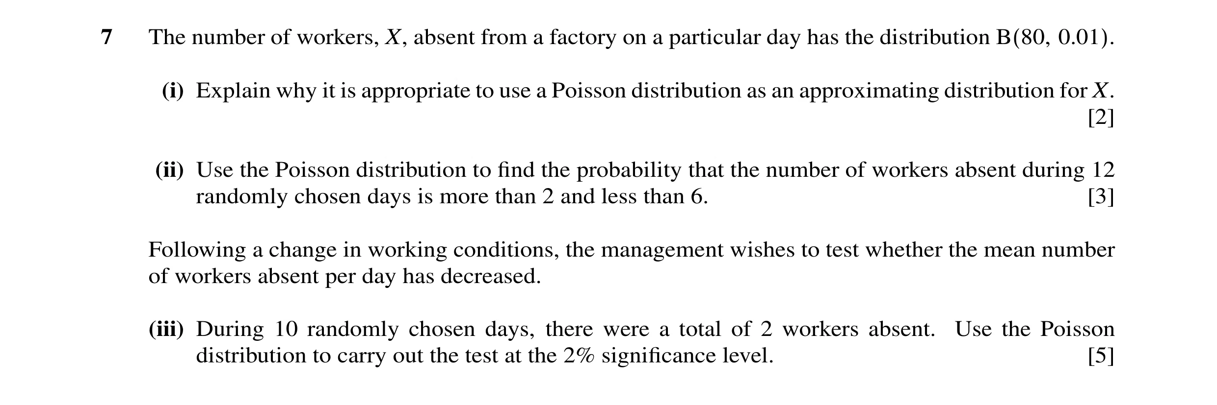
7 The number of workers, X, absent from a factory on a particular day has the distribution B(80, 0.01). (i) Explain why it is appropriate to use a Poisson distribution as an approximating distribution for X. [2] (ii) Use the Poisson distribution to find the probability that the number of workers absent during 12 randomly chosen days is more than 2 and less than 6. [3] Following a change in working conditions, the management wishes to test whether the mean number of workers absent per day has decreased. (iii) During 10 randomly chosen days, there were a total of 2 workers absent. Use the Poisson distribution to carry out the test at the 2% significance level. [5]
10 marks
Mark scheme: 7 (i) n > 50 B1 Accept n large np = 0.8, which is < 5 B1 [2] Accept p small (ii) λ = 9.6 B1 6.9 3 6.9 4 6.9 5 e–9.6( + + ) M1 Any λ Accept end errors. !3 !4 !5 = 0.0800 (3 sfs) A1 [3] Allow 0.08 (iii) H0: Pop mean for 10 days = 8 or Pop mean for 1 day = 0.8 H1: Pop mean for 10 days < 8 B1 Pop mean for 1 day < 0.8 Allow λ or µ but not just ‘mean’ 82 e–8(1 + 8 + ) M1 Any λ. Accept end errors. !2 NB P(2) only used scores M0M0 Accept CR method = 0.0138 or 0.0137 A1 CR = 0, 1, 2 all working must be shown Compare 0.02 M1 Valid comparison with 0.02 or CR Evidence that mean number of A1ft No contradictions absentees has decreased Reject H0 / accept H1 only if H0 / H1 correctly [5] defined Total [10] Total for paper [50]
This question in 9709/73 Oct/Nov 2012
Q15 · Calls arrive at a helpdesk randomly and at a constant average rate of 1.4 calls per hour 9709/73 May/June 2013
6 Calls arrive at a helpdesk randomly and at a constant average rate of 1.4 calls per hour. Calculate the probability that there will be (i) more than 3 calls in 212 hours, [3] (ii) fewer than 1000 calls in four weeks (672 hours). [4]
7 marks
Mark scheme: 6 (i) λ (= 1.4 × 2.5) = 3.5 B1 5.3 2 5.3 3 1 – e-3.5(1 + 3.5 + + ) 2 !3 M1 Any λ allow one end error = 0.463 (3 sf) A1 3 (ii) (λ = 672 × 1.4 = 940.8) N(940.8, 940.8) B1 Seen or implied 9995. − 9408. (= 1.914) 9408. M1 Allow with wrong or no cc . no sd/var Φ(‘1.914’) M1 mixes = 0.972 (3 sf) A1 4 [Total: 7]
This question in 9709/73 May/June 2013
Q16 · On average 1 in 25 000 people have a rare blood condition 9709/73 May/June 2014
1 On average 1 in 25 000 people have a rare blood condition. Use a suitable approximating distribution to find the probability that fewer than 2 people in a random sample of 100 000 have the condition. [3]
3 marks
Mark scheme: 1 e–4(1 + 4) M1 M1 for P (0 or 1) using Poisson, any λ M1 Expression of correct form correct λ (allow 1 end error) = 0.0916 (3 s.f.) A1 [3] SR Use of Bin(100000, 1/25000) scores M1 for P(0,1) allow one end error. A1 0.0916
This question in 9709/73 May/June 2014
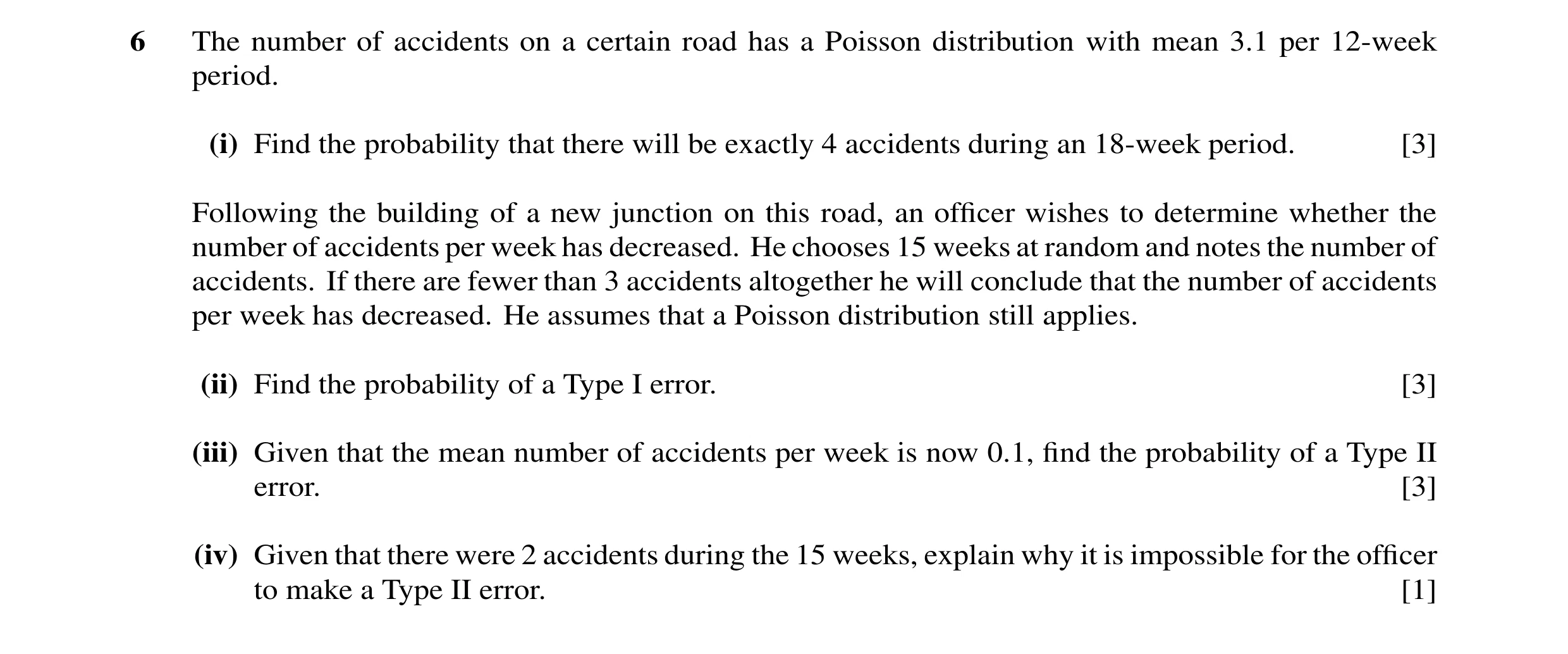
Q17 · The number of accidents on a certain road has a Poisson distribution with mean 3.1 per… 9709/71 Oct/Nov 2014
6 The number of accidents on a certain road has a Poisson distribution with mean 3.1 per 12-week period. (i) Find the probability that there will be exactly 4 accidents during an 18-week period. [3] Following the building of a new junction on this road, an officer wishes to determine whether the number of accidents per week has decreased. He chooses 15 weeks at random and notes the number of accidents. If there are fewer than 3 accidents altogether he will conclude that the number of accidents per week has decreased. He assumes that a Poisson distribution still applies. (ii) Find the probability of a Type I error. [3] (iii) Given that the mean number of accidents per week is now 0.1, find the probability of a Type II error. [3] (iv) Given that there were 2 accidents during the 15 weeks, explain why it is impossible for the officer to make a Type II error. [1]
10 marks
Mark scheme: 6 (i) λ = 4.65 B1 − .4 65 .4 65 4 e × M1 Poisson P(X = 4) with any λ !4 = 0.186 (3 sf) A1 3 (ii) λ = 3.875 B1 − .3 875 .3875 2 P(X = 0, 1, 2) = e 1 + .3875 + = 0.257 (3 sf) M1 Attempted, any λ !2 A1 3 As final answer (iii) λ = 1.5 B1 −5.1 5.1 2 1 – e 1 + 5.1 + M1 1 – P(X = 0, 1, 2) !2 Attempted, any λ = 0.191 (3 sf) A1 3 As final answer (iv) He will reject H0. B1 1 Total: 10
This question in 9709/71 Oct/Nov 2014
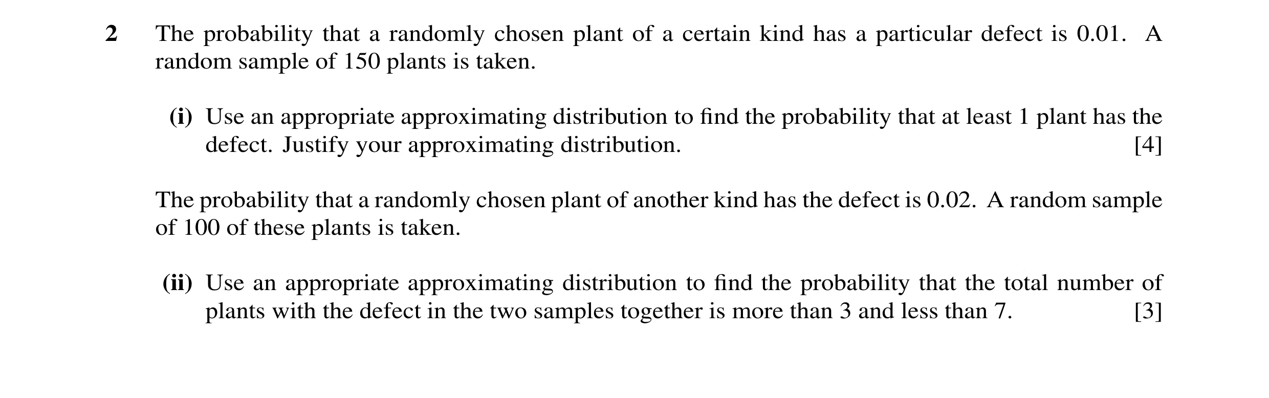
Q18 · The probability that a randomly chosen plant of a certain kind has a particular defect is… 9709/72 Oct/Nov 2014
2 The probability that a randomly chosen plant of a certain kind has a particular defect is 0.01. A random sample of 150 plants is taken. (i) Use an appropriate approximating distribution to find the probability that at least 1 plant has the defect. Justify your approximating distribution. [4] The probability that a randomly chosen plant of another kind has the defect is 0.02. A random sample of 100 of these plants is taken. (ii) Use an appropriate approximating distribution to find the probability that the total number of plants with the defect in the two samples together is more than 3 and less than 7. [3]
7 marks
Mark scheme: 2 (i) (Bin) with n > 50 and mean (or np) < 5 B1 Accept n ‘large’, p ‘small’ Po(1.5) B1 Poisson with correct mean stated or implied 1 – e–1.5 M1 Poisson 1 – P(X = 0); allow incorrect λ; allow 1 end error = 0.777 (3 sf) A1 4 SR If zero scored use of Bin leading to 0.778 / 0.779 scores B1 (ii) 3.5 B1 Correct mean stated or implied − 5.3 5.3 4 5.3 5 5.3 6 M1 Poisson P(X = 4, 5, 6); allow incorrect λ; e + + allow 1 end error !4 !5 !6 = 0.398 (3 sf) A1 3 Total: 7 5.0 2 ( ) ∫
This question in 9709/72 Oct/Nov 2014
Q19 · The number of accidents on a certain road has a Poisson distribution with mean 3.1 per… 9709/72 Oct/Nov 2014
6 The number of accidents on a certain road has a Poisson distribution with mean 3.1 per 12-week period. (i) Find the probability that there will be exactly 4 accidents during an 18-week period. [3] Following the building of a new junction on this road, an officer wishes to determine whether the number of accidents per week has decreased. He chooses 15 weeks at random and notes the number of accidents. If there are fewer than 3 accidents altogether he will conclude that the number of accidents per week has decreased. He assumes that a Poisson distribution still applies. (ii) Find the probability of a Type I error. [3] (iii) Given that the mean number of accidents per week is now 0.1, find the probability of a Type II error. [3] (iv) Given that there were 2 accidents during the 15 weeks, explain why it is impossible for the officer to make a Type II error. [1]
10 marks
Mark scheme: 6 (i) λ = 4.65 B1 − .4 65 .4 65 4 e × M1 Poisson P(X = 4) with any λ !4 = 0.186 (3 sf) A1 3 (ii) λ = 3.875 B1 − .3 875 .3875 2 P(X = 0, 1, 2) = e 1 + .3875 + = 0.257 (3 sf) M1 Attempted, any λ !2 A1 3 As final answer (iii) λ = 1.5 B1 −5.1 5.1 2 1 – e 1 + 5.1 + M1 1 – P(X = 0, 1, 2) !2 Attempted, any λ = 0.191 (3 sf) A1 3 As final answer (iv) He will reject H0. B1 1 Total: 10
This question in 9709/72 Oct/Nov 2014
Q20 · A publishing firm has found that errors in the first draft of a new book occur at random… 9709/71 May/June 2015
6 A publishing firm has found that errors in the first draft of a new book occur at random and that, on average, there is 1 error in every 3 pages of a first draft. Find the probability that in a particular first draft there are (i) exactly 2 errors in 10 pages, [2] (ii) at least 3 errors in 6 pages, [3] (iii) fewer than 50 errors in 200 pages. [4]
9 marks
Mark scheme: 6 (i) 10 2 3 ( 103 ) e −× M1 P(2), allow any λ 2 = 0.198 (3 sf) A1 [2] (ii) − 2 2 2 1 − e 1 + 2 + M1 M1 allow any λ and/or 1end error 2 M1 Correct expression , correct λ = 0.323 (3 sf) A1 [3] (iii) 200 200 N , M1 seen or implied 3 3 495. − 2003 (= –2.102) M1 For standardising allow either wrong or no 200 3 cc No sd/var mix Φ('–2.102') = 1 – Φ('2.102') M1 For finding area consistent with their = 0.0178 (3 sf) A1 [4] working [Total: 9]
This question in 9709/71 May/June 2015
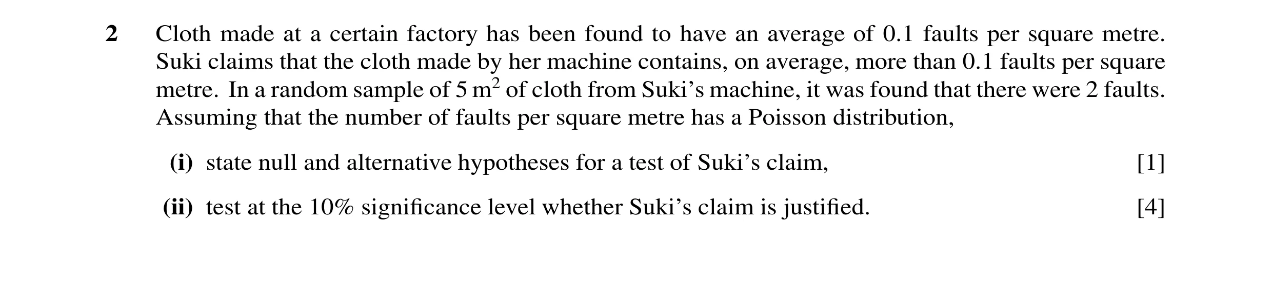
Q21 · Cloth made at a certain factory has been found to have an average of 0.1 faults per… 9709/72 May/June 2015
2 Cloth made at a certain factory has been found to have an average of 0.1 faults per square metre. Suki claims that the cloth made by her machine contains, on average, more than 0.1 faults per square metre. In a random sample of 5 m2 of cloth from Suki’s machine, it was found that there were 2 faults. Assuming that the number of faults per square metre has a Poisson distribution, (i) state null and alternative hypotheses for a test of Suki’s claim, [1] (ii) test at the 10% significance level whether Suki’s claim is justified. [4]
5 marks
Mark scheme: 2 (i) H0: λ = 0.5 or Pop mean = 0.5, not just Mean = 0.5 or Pop mean (per m2 )= 0.1 H1: λ >0.5 B1 1 Accept µ instead of λ (ii) 1 – e–0.5(1 + 0.5) M1 1 – P(X = 0,1) attempted, any λ. Allow 1 end error = 0.0902 (3 sf) A1 Allow 0.09 comp 0.1 M1 Valid comparison NB 0.9098>0.9 recovers M1A1 M1 Claim justified or there is evidence to oe Accept ‘Reject H0’ if correctly defined support claim A1 4 No contradictions. Total 5
This question in 9709/72 May/June 2015
Q22 · In a golf tournament, the number of times in a day that a ‘hole-in-one’ is scored is… 9709/72 May/June 2015
3 In a golf tournament, the number of times in a day that a ‘hole-in-one’ is scored is denoted by the variable X, which has a Poisson distribution with mean 0.15. Mr Crump offers to pay $200 each time that a hole-in-one is scored during 5 days of play. Find the expectation and variance of the amount that Mr Crump pays. [5]
5 marks
Mark scheme: 3 λ = 5×0.15 (= 0.75) M1 E(amount) = 200×0.75 = 150 A1 Var(weekly no of hole–in–ones) = 0.75 B1 Var(amount) = 2002 × 0.75 M1 Allow 2002 × their variance (with nothing = 30,000 A1 5 added/subtracted at any stage) (SR probability table can score M1A0 srB1 if var rounds to 30,000 (2sf) ) Total 5
This question in 9709/72 May/June 2015
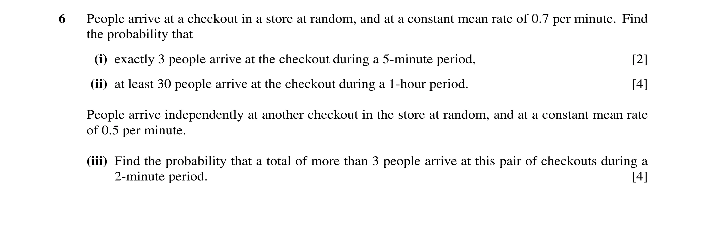
Q23 · People arrive at a checkout in a store at random, and at a constant mean rate of 0.7 per… 9709/73 May/June 2015
6 People arrive at a checkout in a store at random, and at a constant mean rate of 0.7 per minute. Find the probability that (i) exactly 3 people arrive at the checkout during a 5-minute period, [2] (ii) at least 30 people arrive at the checkout during a 1-hour period. [4] People arrive independently at another checkout in the store at random, and at a constant mean rate of 0.5 per minute. (iii) Find the probability that a total of more than 3 people arrive at this pair of checkouts during a 2-minute period. [4]
10 marks
Mark scheme: − 5.3 5.3 6 (i) e × M1 P(X = 3) any λ !3 = 0.216 (3 sf) A1 [2] (ii) N(42, 42) stated or implied B1 29 5. − 42 (= –1.929) M1 Allow with wrong or no cc OR without √ 42 P(z > ‘–1.929’) = Φ(‘1.929’) M1 For correct area consistent with their working = 0.973 (3 sf) A1 [4] (iii) (λ) = 2.4 B1 − 4.2 4.2 2 4.2 3 1 − e 1 + 4.2 + + M1 for 1 – P(X Y 3), any λ allow one end error 2 !3 M1 Correct expression any λ = 0.221 (3 sf) A1 4 NB For combination method B1 attempting 10 combinations with λ=1, λ=1.4 M1 6 expressions M1 10 expressions 0.221 A1 Total 10
This question in 9709/73 May/June 2015
Q24 · Failures of two computers occur at random and independently 9709/71 Oct/Nov 2015
1 Failures of two computers occur at random and independently. On average the first computer fails 1.2 times per year and the second computer fails 2.3 times per year. Find the probability that the total number of failures by the two computers in a 6-month period is more than 1 and less than 4. [4]
4 marks
Mark scheme: 1 λ= (1.2 + 2.3) ÷ 2 M1 Attempt combined mean, allow 1.2 + 2.3 A1 Correct mean = 1.75 .1 75 2 .175 3 M1 Allow incorrect mean. + e–1.75 2 !3 Allow end errors (1 and/or 4) = 0.421 (3 sf) A1 [4] Total: 4 6
This question in 9709/71 Oct/Nov 2015
Q25 · Failures of two computers occur at random and independently 9709/72 Oct/Nov 2015
1 Failures of two computers occur at random and independently. On average the first computer fails 1.2 times per year and the second computer fails 2.3 times per year. Find the probability that the total number of failures by the two computers in a 6-month period is more than 1 and less than 4. [4]
4 marks
Mark scheme: 1 λ= (1.2 + 2.3) ÷ 2 M1 Attempt combined mean, allow 1.2 + 2.3 A1 Correct mean = 1.75 .1 75 2 .175 3 M1 Allow incorrect mean. + e–1.75 2 !3 Allow end errors (1 and/or 4) = 0.421 (3 sf) A1 [4] Total: 4 6
This question in 9709/72 Oct/Nov 2015
Q26 · On average, 1 in 2500 adults has a certain medical condition 9709/72 Oct/Nov 2015
5 On average, 1 in 2500 adults has a certain medical condition. (i) Use a suitable approximation to find the probability that, in a random sample of 4000 people, more than 3 have this condition. [3] (ii) In a random sample of n people, where n is large, the probability that none has the condition is less than 0.05. Find the smallest possible value of n. [4]
7 marks
Mark scheme: 5 (i) Po(1.6) stated or implied M1 6.1 2 6.1 3 M1 + P ( X > 3) = 1 − e −6.1 1 + 6.1 + Allow M1 for 1 – P(X ⩽3), incorrect λ 2 !3 and allow one end error A1 [3] SR Use of Bin scores B1 only for 0.0788 = 0.0788 (3 sf) n or or (ii) B1 µ λ = -e 2500 < 0.05 M1 2499 B1 n 2500 − e 2500 < .005 Allow = M1 n 2499 Allow incorrect λ < .005 2500 M1 2499 n M1 –µ < ln 0.05 M1 nln < ln .005 − < ln .005 Attempt ln bs 2500 (µ > 2.9957) 2500 n > 7489.3 (1 dp) M1 Smallest n = 7490 A1 [4] n = µ × 2500 B1 Smallest n = 7488 Smallest n = 7490 A1 A1 Total: 7
This question in 9709/72 Oct/Nov 2015
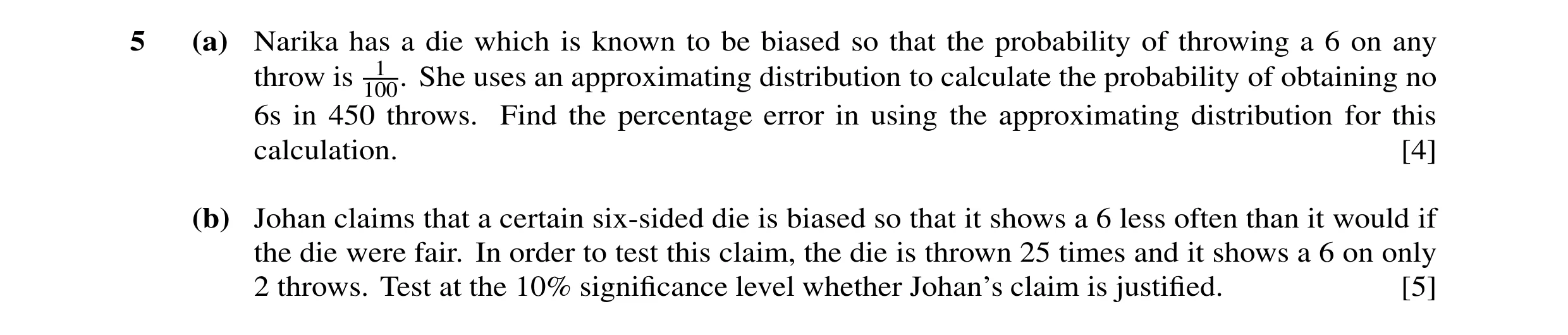
Q27 · Narika has a die which is known to be biased so that the probability of throwing a 6 on… 9709/73 Oct/Nov 2015
5 (a) Narika has a die which is known to be biased so that the probability of throwing a 6 on any throw is 100.1 She uses an approximating distribution to calculate the probability of obtaining no 6s in 450 throws. Find the percentage error in using the approximating distribution for this calculation. [4] (b) Johan claims that a certain six-sided die is biased so that it shows a 6 less often than it would if the die were fair. In order to test this claim, the die is thrown 25 times and it shows a 6 on only 2 throws. Test at the 10% significance level whether Johan’s claim is justified. [5]
9 marks
Mark scheme: 25 24 23 2 25 5 5 1 5 1
This question in 9709/73 Oct/Nov 2015
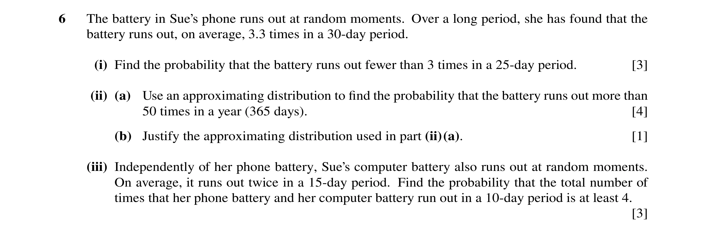
Q28 · The battery in Sue’s phone runs out at random moments 9709/72 Feb/March 2016
6 The battery in Sue’s phone runs out at random moments. Over a long period, she has found that the battery runs out, on average, 3.3 times in a 30-day period. (i) Find the probability that the battery runs out fewer than 3 times in a 25-day period. [3] (ii) (a) Use an approximating distribution to find the probability that the battery runs out more than 50 times in a year (365 days). [4] (b) Justify the approximating distribution used in part (ii)(a). [1] (iii) Independently of her phone battery, Sue’s computer battery also runs out at random moments. On average, it runs out twice in a 15-day period. Find the probability that the total number of times that her phone battery and her computer battery run out in a 10-day period is at least 4. [3]
11 marks
Mark scheme: 6 (i) λ = 3.3 × 3025 = 2.75 B1 e–2.75(1 + 2.75 + 2.752 2 ) M1 Allow any λ Allow one end error = 0.481 (3 sf) A1 [3] As final answer. Accept 0.482 (ii) (a) λ (= 3.3 × 36530 ) = 40.15 B1 Accept 40.1 or 40.2 (X ~ Po(40.15) ⇒X ~ N(40.15, 40.15)) 50.5 −"40.15" (= 1.633) M1 Allow with incorrect or no cc OR no √ sign "40.15" 1 – Φ("1.633") M1 For correct area consistent with their working = 0.0513 (3 sf) A1 [4] Accept 0.0512 (b) λ > 15 B1 [1] or similar (iii) λ = 3073 oe or 1.1+1.33= 2.43 (3 sf) B1 1 – e–2.43(1 + 2.43 + 2.432 2 + 2.433! 3 ) M1 Allow any λ. Allow one end error = 0.228 (3 sf) A1 [3]
This question in 9709/72 Feb/March 2016
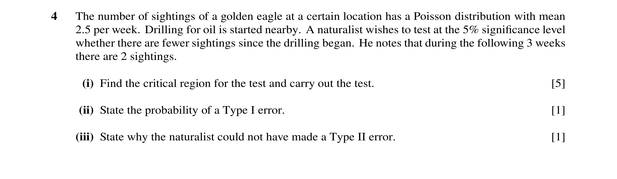
Q29 · The number of sightings of a golden eagle at a certain location has a Poisson… 9709/73 May/June 2016
4 The number of sightings of a golden eagle at a certain location has a Poisson distribution with mean 2.5 per week. Drilling for oil is started nearby. A naturalist wishes to test at the 5% significance level whether there are fewer sightings since the drilling began. He notes that during the following 3 weeks there are 2 sightings. (i) Find the critical region for the test and carry out the test. [5] (ii) State the probability of a Type I error. [1] (iii) State why the naturalist could not have made a Type II error. [1]
7 marks
Mark scheme: 4 (i) H0: Pop mean = 2.5 (or 7.5) or λ = 2.5(Not just “mean”) Allow µ H0: Pop mean < 2.5 (or 7.5) B1 or λ < 2.5 λ = 7.5 P(X ⩽ 2) = e–7.5(1+7.5+ 7.52 2 ) = 0.0203 3 M1 Either P(X⩽2) or P(X⩽3) , allow any λ P(X⩽3)=0.0203 + e–7.5× 7.53! = 0.0591 A1 Both Correct CR is X ⩽ 2 A1 Clear statement Reject H0 A1 [5] Follow through their CR/their P(X⩽2) Evidence that no of sightings fewer (ii) P(Type I) = 0.0203 (3 sf) B1 [1] ft their P(X ⩽ 2) (iii) H0 was rejected oe B1 [1] or Type II is P(not reject H0)oe
This question in 9709/73 May/June 2016
Q30 · Particles are emitted randomly from a radioactive substance at a constant average rate of… 9709/71 Oct/Nov 2016
3 Particles are emitted randomly from a radioactive substance at a constant average rate of 3.6 per minute. Find the probability that (i) more than 3 particles are emitted during a 20-second period, [3] (ii) more than 240 particles are emitted during a 1-hour period. [4]
7 marks
Mark scheme: 3 (i) (λ) = 3.6 ÷ 3 = 1.2 B1 1.2 seen M1 Allow any λ 1 − e −1.2 ( 1 + 1.2 + 1.22 2 + 1.23!3 ) = 0.0338 (3 sf) A1 [3] As final answer (ii) N(60 × 3.6, 60 × 3.6) M1 Stated or implied 240.5 − '216' (= 1.667) M1 Allow with no or wrong cc (no sd/var mixes) '216' 1– Φ(‘1.667’) M1 Area consistent with their working = 0.0478 (3 sf) A1 [4] SR use of Poisson 0.0497 scores 4/4
This question in 9709/71 Oct/Nov 2016
Q31 · Particles are emitted randomly from a radioactive substance at a constant average rate of… 9709/72 Oct/Nov 2016
3 Particles are emitted randomly from a radioactive substance at a constant average rate of 3.6 per minute. Find the probability that (i) more than 3 particles are emitted during a 20-second period, [3] (ii) more than 240 particles are emitted during a 1-hour period. [4]
7 marks
Mark scheme: 3 (i) (λ) = 3.6 ÷ 3 = 1.2 B1 1.2 seen M1 Allow any λ 1 − e −1.2 ( 1 + 1.2 + 1.22 2 + 1.23!3 ) = 0.0338 (3 sf) A1 [3] As final answer (ii) N(60 × 3.6, 60 × 3.6) M1 Stated or implied 240.5 − '216' (= 1.667) M1 Allow with no or wrong cc (no sd/var mixes) '216' 1– Φ(‘1.667’) M1 Area consistent with their working = 0.0478 (3 sf) A1 [4] SR use of Poisson 0.0497 scores 4/4
This question in 9709/72 Oct/Nov 2016
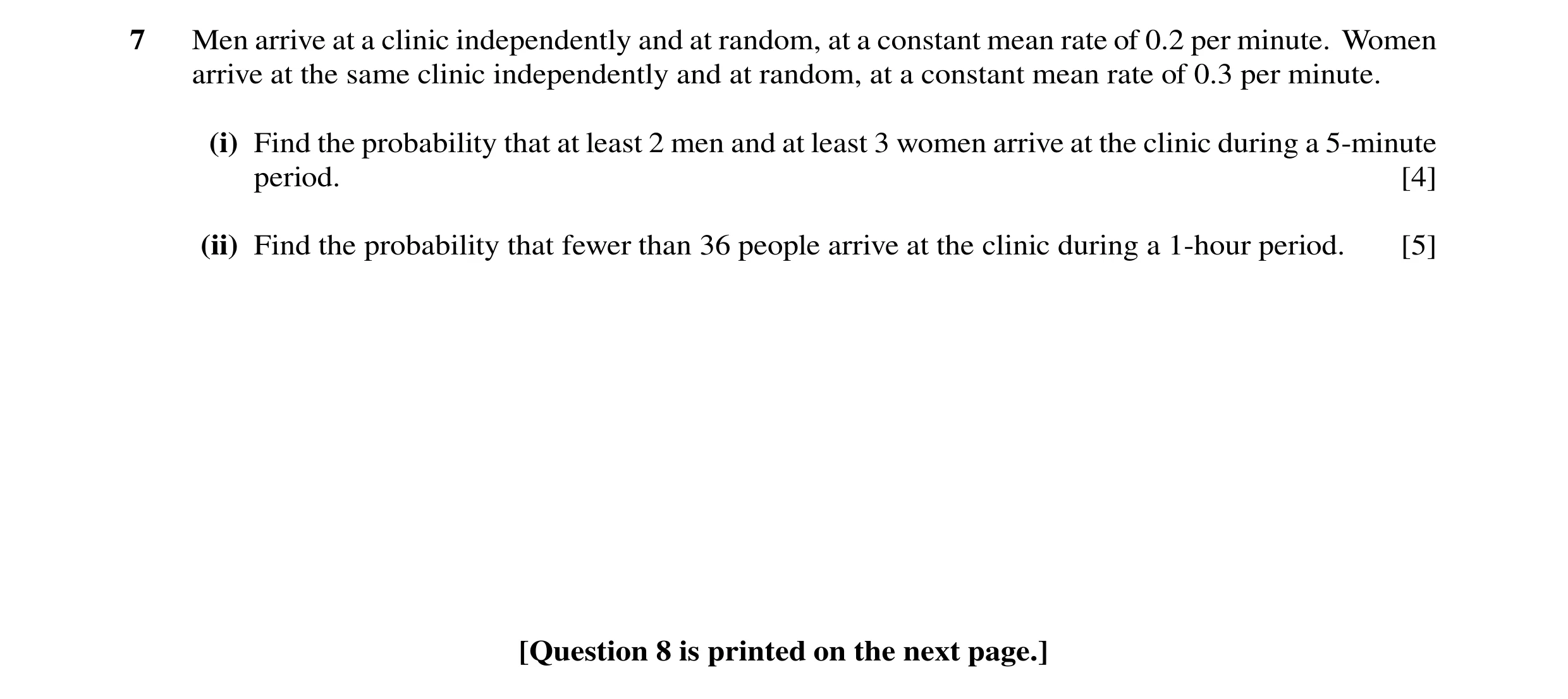
Q32 · Men arrive at a clinic independently and at random, at a constant mean rate of 0.2 per… 9709/73 Oct/Nov 2016
7 Men arrive at a clinic independently and at random, at a constant mean rate of 0.2 per minute. Women arrive at the same clinic independently and at random, at a constant mean rate of 0.3 per minute. (i) Find the probability that at least 2 men and at least 3 women arrive at the clinic during a 5-minute period. [4] (ii) Find the probability that fewer than 36 people arrive at the clinic during a 1-hour period. [5] [Question 8 is printed on the next page.]
9 marks
Mark scheme: 7 (i) 1 – e–1 (1 + 1) (= 0.26424) B1 B1 for either λ correct. 1 – e–1.5 (1 + 1.5 + 1.52!2 ) (= 0.19115) B1 B1 for either correct expression with correct λ ‘0.26424’ × ‘0.19115’ M1 product of their values for ⩽ 2 and ⩽ 3 from Poisson, need correct form “ 1 - .. “ , but allow incorrect λ values and end errors = 0.0505 (3 sf) A1 accept 0.0504 [4] (ii) λ = 30 B1 N(30, 30) B1 seen or implied, need N(λ,λ) 35.5 − 30 (= 1.004) M1 allow with wrong or no cc or no √ 30 Φ (‘1.004’) M1 consistent with their working = 0.842 (3 sf) A1 [5]
This question in 9709/73 Oct/Nov 2016
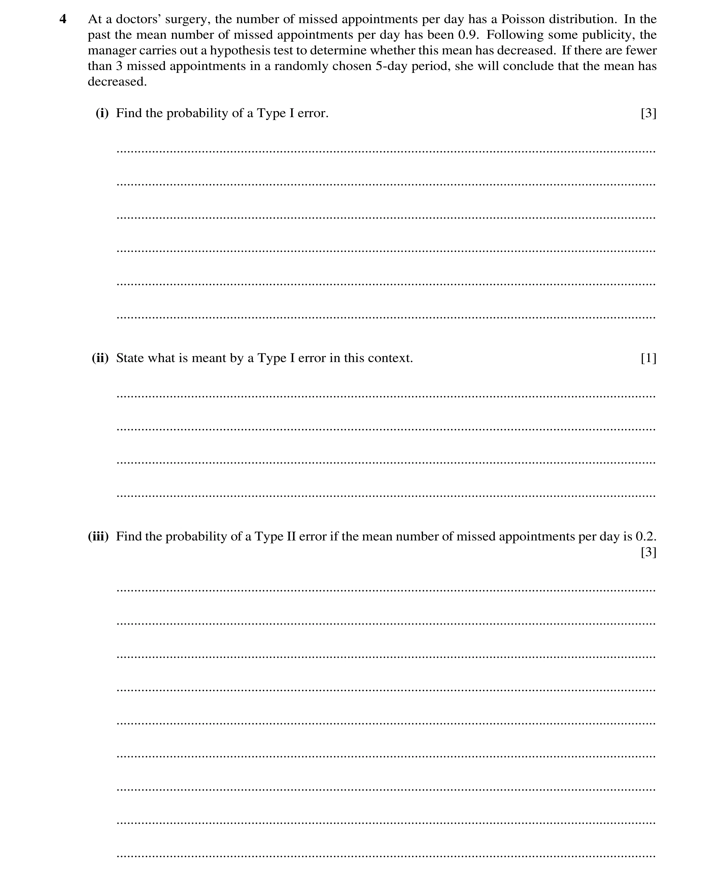
Q33 · At a doctors’ surgery, the number of missed appointments per day has a Poisson… 9709/72 Feb/March 2017
4 At a doctors’ surgery, the number of missed appointments per day has a Poisson distribution. In the past the mean number of missed appointments per day has been 0.9. Following some publicity, the manager carries out a hypothesis test to determine whether this mean has decreased. If there are fewer than 3 missed appointments in a randomly chosen 5-day period, she will conclude that the mean has decreased. (i) Find the probability of a Type I error. [3] … … … … … … (ii) State what is meant by a Type I error in this context. [1] … … … … (iii) Find the probability of a Type II error if the mean number of missed appointments per day is 0.2. [3] … … … … … … … … …
7 marks
Mark scheme: 4(i) (λ =) 4.5 B1 e–4.5(1 + 4.5 + 4.52!2 ) M1 Allow any λ. Allow one end error = 0.174 A1 Total: 3 4(ii) Accept reduction in mean no. of B1 or Mean is 0.9 (or 4.5) but < 3 missed missed appts although untrue appts. In context Total: 1 4(iii) P(X ⩾ 3) M1 Attempted = 1 – e–1(1 + 1 + 212! ) M1 Allow any λ except 4.5 or 0.9, Allow one end error = 0.0803 (3 sfs) A1 Total: 3
This question in 9709/72 Feb/March 2017
Q34 · The number of planes arriving at an airport every hour during daytime is modelled by the… 9709/72 Feb/March 2017
7 The number of planes arriving at an airport every hour during daytime is modelled by the random variable X with distribution Po 5.2 . (i) State two assumptions required for the Poisson model to be valid in this context. [2] … … … … (ii) (a) Find the probability that the number of planes arriving in a 15-minute period is greater than 1 and less than 4, [3] … … … … … … … … … (b) Find the probability that more than 3 planes will arrive in a 40-minute period. [2] … … … … … … … … (iii) The airport has enough staffto deal with a maximum of 60 planes landing during a 10-hour day. Use a suitable approximation to find the probability that, on a randomly chosen 10-hour day, staffwill be able to deal with all the planes that land. [4] … … … … … … … … … … … … … … … … … … … … … … … …
11 marks
Mark scheme: 7(i) Planes arrive at constant mean rate B1 Planes arrive at random B1 or Planes arrive independently Must be in context Total: 2 7(ii)(a) (λ =) 5.2 ÷ 4 M1 e–1.3( 1.32 2 + 1.33!3 ) M1 Allow any λ , allow one end error = 0.330 (3 sfs) A1 Accept 0.33 Total: 3 7(ii)(b) 1– e–3.467×(1+3.467 + 3.4672! 2 + 3.4673! 3 ) M1 Allow any λ except 5.2 or 1.3, allow one end error = 0.456 (3 sfs) A1 Total: 2 7(iii) N(52, 52) stated or implied B1 60.5 − 52 (= 1.179) M1 ft their mean and var. 52 Allow wrong or no cc or no √ Φ(“1.179”) M1 = 0.881 (3 sf) A1 Total: 4
This question in 9709/72 Feb/March 2017
Q35 · On average, 1 clover plant in 10 000 has four leaves instead of three 9709/71 May/June 2017
1 On average, 1 clover plant in 10 000 has four leaves instead of three. (i) Use an approximating distribution to calculate the probability that, in a random sample of 2000 clover plants, more than 2 will have four leaves. [3] … … … … … … … … … … … … … … … … (ii) Justify your approximating distribution. [2] … … … … … …
5 marks
Mark scheme: 1(i) B1 1−e−0.2 (1 + 0.2 + 2 0.2 2 ) M1 1 – Poisson P(0, 1, 2, 3) attempted, any λ, allow one end error = 0.00115 (3 sf) A1 SR: using Bin, ans 0.00115: B1 Total: 3 1(ii) n large (n > 50) B1 np = 0.2 < 5 or p small B1 Total: 2
This question in 9709/71 May/June 2017
Q36 · The number of sports injuries per month at a certain college has a Poisson distribution 9709/71 May/June 2017
6 The number of sports injuries per month at a certain college has a Poisson distribution. In the past the mean has been 1.1 injuries per month. The principal recently introduced new safety guidelines and she decides to test, at the 2% significance level, whether the mean number of sports injuries has been reduced. She notes the number of sports injuries during a 6-month period. (i) Find the critical region for the test and state the probability of a Type I error. [6] … … … … … … … … … … … … … … … (ii) State what is meant by a Type I error in this context. [1] … … … … … … (iii) During the 6-month period there are a total of 2 sports injuries. Carry out the test. [3] … … … … … … … … … (iv) Assuming that the mean remains 1.1, calculate the probability that there will be fewer than 30 sports injuries during a 36-month period. [4] … … … … … … … … … … … … … …
14 marks
Mark scheme: 6(i) mean = 6.6 B1 B1 for 6.6 (could be scored in iii) P(X ⩽ 1) = e–6.6 (1 + 6.6) = 0.0103 M1 Allow incorrect λ in both probs P(X ⩽ 2) = e–6.6(1 + 6.6 + 2 6.6 2 )= 0.0400 M1A1 A1 for both values CR is X ⩽ 1 DA1 Dep on at least one M P(Type I error) = P(X ⩽ 1) = 0.0103 B1FT FT their P(X ⩽ 1) Total: 6 6(ii) Wrongly concluding that (mean) no of (sports) injuries has decreased B1 Must be in context Total: 1 Question Answer Marks Guidance 6(iii) H0: λ = 6.6 H1: λ < 6.6 B1 Can be scored in (i). Allow µ or λ / 1.1 or 6.6 or P(X ⩽ 2) = 0.0400 > 0.02 2 not in CR M1 No evidence mean no. of injuries has decreased A1FT Total: 3 6(iv) N(39.6, 39.6) B1 May be implied 29.5 39.6 39.6 − (= −1.605) M1 Allow with wrong or no cc Φ(“–1.605”) = 1 – Φ(“1.605”) M1 For area consistent with their mean = 0.0543 (3 sfs) A1 Total: 4
This question in 9709/71 May/June 2017
Q37 · Old televisions arrive randomly and independently at a recycling centre at an average… 9709/72 May/June 2017
6 Old televisions arrive randomly and independently at a recycling centre at an average rate of 1.2 per day. (i) Find the probability that exactly 2 televisions arrive in a 2-day period. [2] … … … … … … … … (ii) Use an appropriate approximating distribution to find the probability that at least 55 televisions arrive in a 50-day period. [4] … … … … … … … … … … … … … … Independently of televisions, old computers arrive randomly and independently at the same recycling centre at an average rate of 4 per 7-day week. (iii) Find the probability that the total number of televisions and computers that arrive at the recycling centre in a 3-day period is less than 4. [3] … … … … … … … … … … … … … … … … … … … … … … …
9 marks
Mark scheme: 6(i) 2 2.4 2.4 2! e− × M1 = 0.261 (3 sfs) A1 Total: 2 6(ii) N(60, 60) B1 seen or implied 54.5 60 60 − (= ̶ 0.710) M1 allow with wrong or missing cc 1 ̶ φ(" ̶ 0.710") = φ("0.710") M1 For area consistent with their working = 0.761 (3 sf) A1 Total: 4 6(iii) λ = 3.6 + 12 ÷ 7 (= 186/35) (= 5.314) M1 ( ) 2 3 5.314 5.314 5.314 2 3! 1 5.314 e− + + + M1 Allow incorrect λ. Allow one end error. = 0.224 (3 sfs) A1 Total: 3
This question in 9709/72 May/June 2017
Q38 · In the past the number of accidents per month on a certain road was modelled by a random… 9709/73 May/June 2017
7 In the past the number of accidents per month on a certain road was modelled by a random variable with distribution Po 0.47 . After the introduction of speed restrictions, the government wished to test, at the 5% significance level, whether the mean number of accidents had decreased. They noted the number of accidents during the next 12 months. It is assumed that accidents occur randomly and that a Poisson model is still appropriate. (i) Given that the total number of accidents during the 12 months was 2, carry out the test. [6] … … … … … … … … … … … … … … … … … … … … … … (ii) Explain what is meant by a Type II error in this context. [1] … … … … It is given that the mean number of accidents per month is now in fact 0.05. (iii) Using another random sample of 12 months the same test is carried out again, with the same significance level. Find the probability of a Type II error. [4] … … … … … … … … … … … … … … … … … …
11 marks
Mark scheme: 7(i) H0: Pop mean no. accidents = 5.64 H1: Pop mean no. accidents < 5.64 B1 not just "mean", but allow just "λ" or “µ” Use of λ = 5.64 B1 used in a Poisson calculation = e−5.64 (1 + 5.64 + 2 5.64 2 ) M1 Allow incorrect λ in otherwise correct = 0.08(0) A1 Comp with 0.05 M1 Valid comparison (Poisson only), no contradictions. No evidence to believe mean no. of accidents has decreased; accept H0 (if correctly defined) A1FT Normal distribution: M0M0 Total: 6 7(ii) Mean < 0.47 but conclude that this is not so B1 (Mean) no. of accidents reduced, but conclude not reduced. Must be in context. Total: 1 7(iii) (Need greatest x such that P(X ⩽ x) < 0.05 ) P(X ⩽ 1) = e−5.64 (1 + 5.64) = 0.024 P(X ⩽ 2) = 0.08 B1 Both, could be seen in (i) Hence rejection region is X ⩽ 1 B1 Can be implied With λ = 12× 0.05 = 0.6, 1 ̶ P(X ⩽ 1) = 1 ̶ e−0.6(1+ 0.6) M1 λ=0.6 and 1 ̶ P(X ⩽ 1) = 0.122 (3 sf) A1 Normal scores 0 Total: 4
This question in 9709/73 May/June 2017
Q39 · In a certain factory the number of items per day found to be defective has had the… 9709/72 Oct/Nov 2017
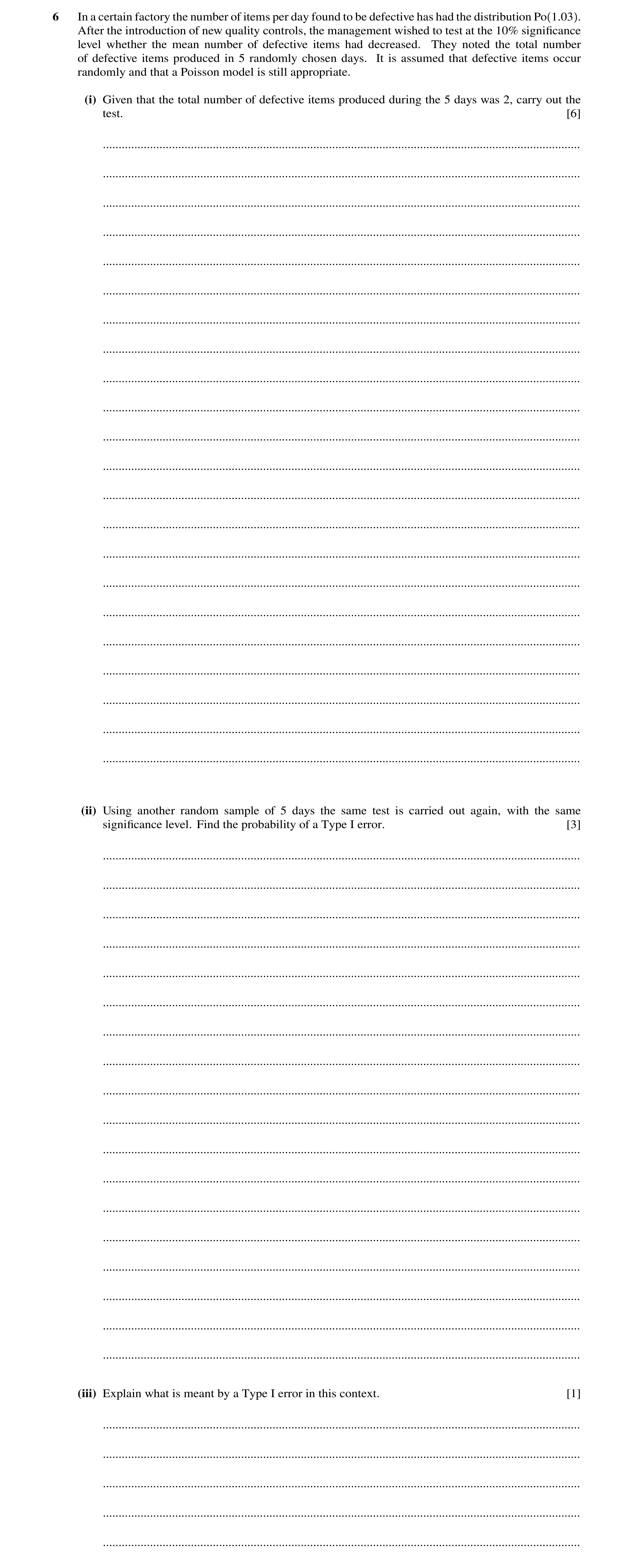
6 In a certain factory the number of items per day found to be defective has had the distribution Po 1.03 . After the introduction of new quality controls, the management wished to test at the 10% significance level whether the mean number of defective items had decreased. They noted the total number of defective items produced in 5 randomly chosen days. It is assumed that defective items occur randomly and that a Poisson model is still appropriate. (i) Given that the total number of defective items produced during the 5 days was 2, carry out the test. [6] … … … … … … … … … … … … … … … … … … … … … … (ii) Using another random sample of 5 days the same test is carried out again, with the same significance level. Find the probability of a Type I error. [3] … … … … … … … … … … … … … … … … … … (iii) Explain what is meant by a Type I error in this context. [1] … … … … …
10 marks
Mark scheme: 6(i) H0: Pop mean no. defectives = 5.15 H1: Pop mean no. defectives < 5.15 B1 or ‘= 1.03 (per day)’ not just ‘mean’, but allow just ‘λ’ or ‘µ’ P(X ⩽ 2) M1 Attempted. Any one term error/end error/incorrect λ/expression 1–… = e−5.15 (1 + 5.15 + 2 15 .5 2 ) M1 Correct expression attempted = 0.113 A1 Comp with 0.1 M1 Valid comparison No evidence to believe mean no. of defectives has decreased A1 FT Correct conclusion (FT their value) No contradictions 6 Question Answer Marks Guidance 6(ii) BOTH P(X ⩽ 1) = e−5.15 (1 + 5.15) (= 0.0357) AND P(X ⩽ 2) = = e−5.15 (1 + 5.15 + 2 15 .5 2 )= (0.113) B1* (Could be seen in (i)) Comp either with 0.1 DB1 One comparison with 0.01 (could be seen in (i)) P(Type I error) = 0.0357 (3 sf) B1 3 6(iii) Actually mean = 1.03 but conclude that mean < 1.03 B1 Mean no. of defectives not reduced, but conclude that it is reduced. 1
This question in 9709/72 Oct/Nov 2017
Q40 · The number of absences by girls from a certain class on any day is modelled by a random… 9709/71 May/June 2018
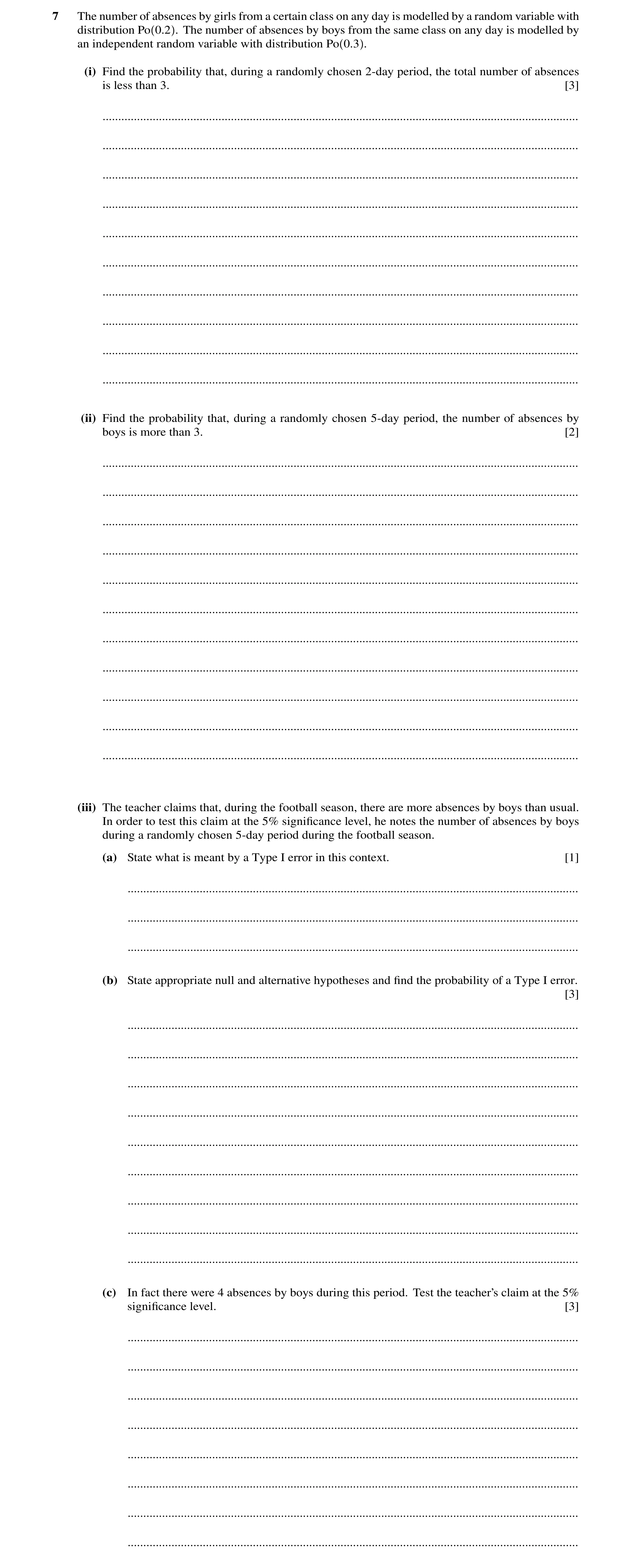
7 The number of absences by girls from a certain class on any day is modelled by a random variable with distribution Po 0.2 . The number of absences by boys from the same class on any day is modelled by an independent random variable with distribution Po 0.3 . (i) Find the probability that, during a randomly chosen 2-day period, the total number of absences is less than 3. [3] … … … … … … … … … … (ii) Find the probability that, during a randomly chosen 5-day period, the number of absences by boys is more than 3. [2] … … … … … … … … … … … (iii) The teacher claims that, during the football season, there are more absences by boys than usual. In order to test this claim at the 5% significance level, he notes the number of absences by boys during a randomly chosen 5-day period during the football season. (a) State what is meant by a Type I error in this context. [1] … … … (b) State appropriate null and alternative hypotheses and find the probability of a Type I error. [3] … … … … … … … … … (c) In fact there were 4 absences by boys during this period. Test the teacher’s claim at the 5% significance level. [3] … … … … … … … …
12 marks
Mark scheme: 7(i) Po(1.0) B1 Seen or implied e–1 (1 + 1 + 122 ) M1 Allow any λ. Allow one end error. = 0.920 (3 sfs) A1 3 7(ii) P(X > 3) = 1 – e–1.5(1+1.5+ 1.52 2 + 1.53!3 ) M1 Allow any λ. Allow one end error = 0.0656 A1 2 7(iii)(a) Incorrectly concluding that more absences B1 In context than usual when there are not oe 1 7(iii)(b) H0: λ = 1.5 (or 0.3) B1 Or µ H1: λ > 1.5 (or 0.3) Both P(X > 4) = “0.0656” – e–1.5 × 1.54!4 M1 or 1 – e–1.5(1+1.5+ 1.52 2 + 1.53!3 + 1.54!4 ) = 0.0186 (3 sf) P(Type I) = 0.0186 or 0.0185 A1ft Ft their P(X > 4) if less than 0.05 3 7(iii)(c) P(X > 3) = "0.0656" B1ft Ft their (ii) 0.0656 > 0.05 M1 No evidence of more than usual male A1ft Ft their P(X>3). Correct conclusion. absences No contradictions. 3
This question in 9709/71 May/June 2018
Q41 · Accidents on a particular road occur at a constant average rate of 1 every 4.8 weeks 9709/72 May/June 2018
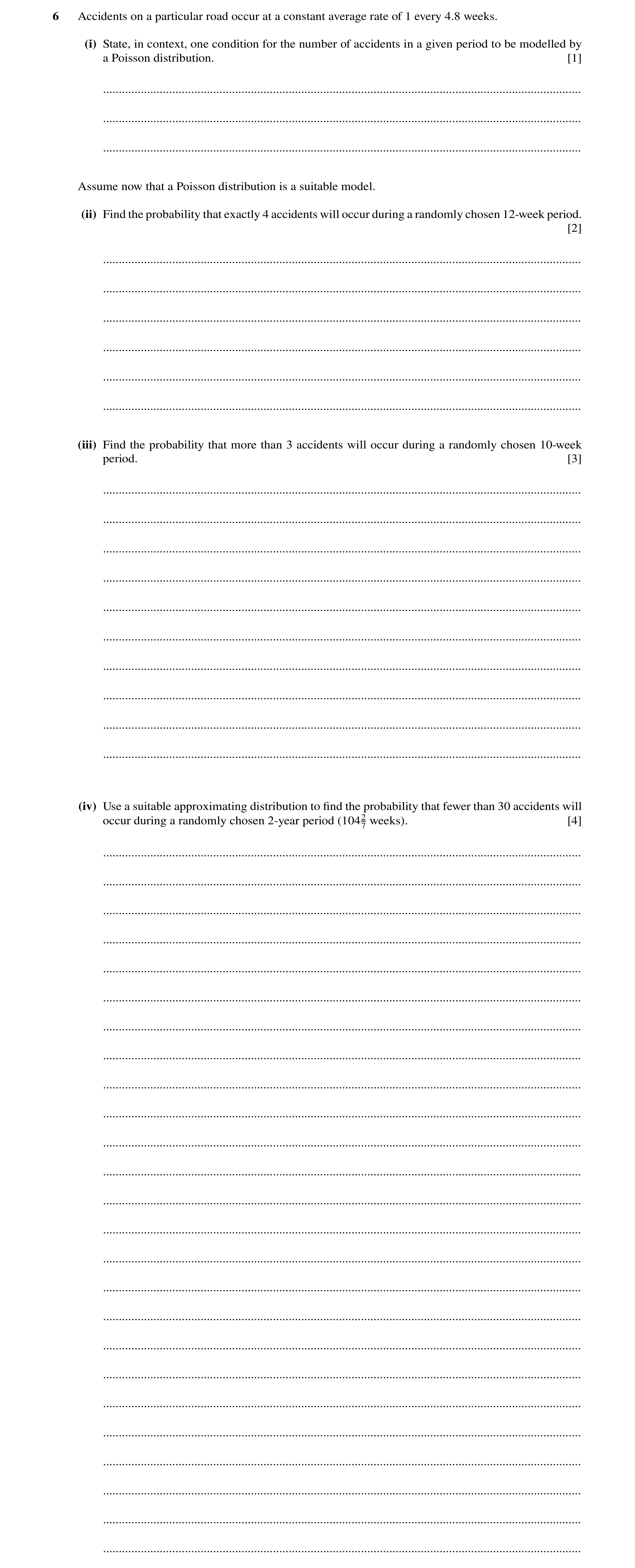
6 Accidents on a particular road occur at a constant average rate of 1 every 4.8 weeks. (i) State, in context, one condition for the number of accidents in a given period to be modelled by a Poisson distribution. [1] … … … Assume now that a Poisson distribution is a suitable model. (ii) Find the probability that exactly 4 accidents will occur during a randomly chosen 12-week period. [2] … … … … … … (iii) Find the probability that more than 3 accidents will occur during a randomly chosen 10-week period. [3] … … … … … … … … … … (iv) Use a suitable approximating distribution to find the probability that fewer than 30 accidents will occur during a randomly chosen 2-year period (1042 weeks). [4] 7 … … … … … … … … … … … … … … … … … … … … … … … … …
10 marks
Mark scheme: 6(i) Accidents occur independently or randomly B1 In context. Allow ‘singly’. 1 6(ii) e–2.5 × 4 2.5 4! M1 Poisson P(4), allow any λ = 0.134 (3 sfs) A1 2 Question Answer Marks Guidance 6(iii) λ = 25 12 or 2.08(333) B1 1 – 25 12 e − (1 + 25 12 + 2 25 12 2! + 3 25 12 3! ) M1 1 – Poisson P(0, 1, 2, 3), allow any λ allow one end error = 0.158 (3 sfs) A1 As final answer 3 6(iv) N(1825 84 ,1825 84 ) or N(21.7(26), 21.7(26)) B1 Stated or implied 1825 29.5 84 1825 84 − M1 Allow with wrong or no cc with their mean/sd Φ(“1.668”) M1 Correct area consistent with their working = 0.952 ( 3 sfs) A1 4
This question in 9709/72 May/June 2018
Q42 · The numbers, M and F, of male and female students who leave a particular school each year… 9709/73 May/June 2018
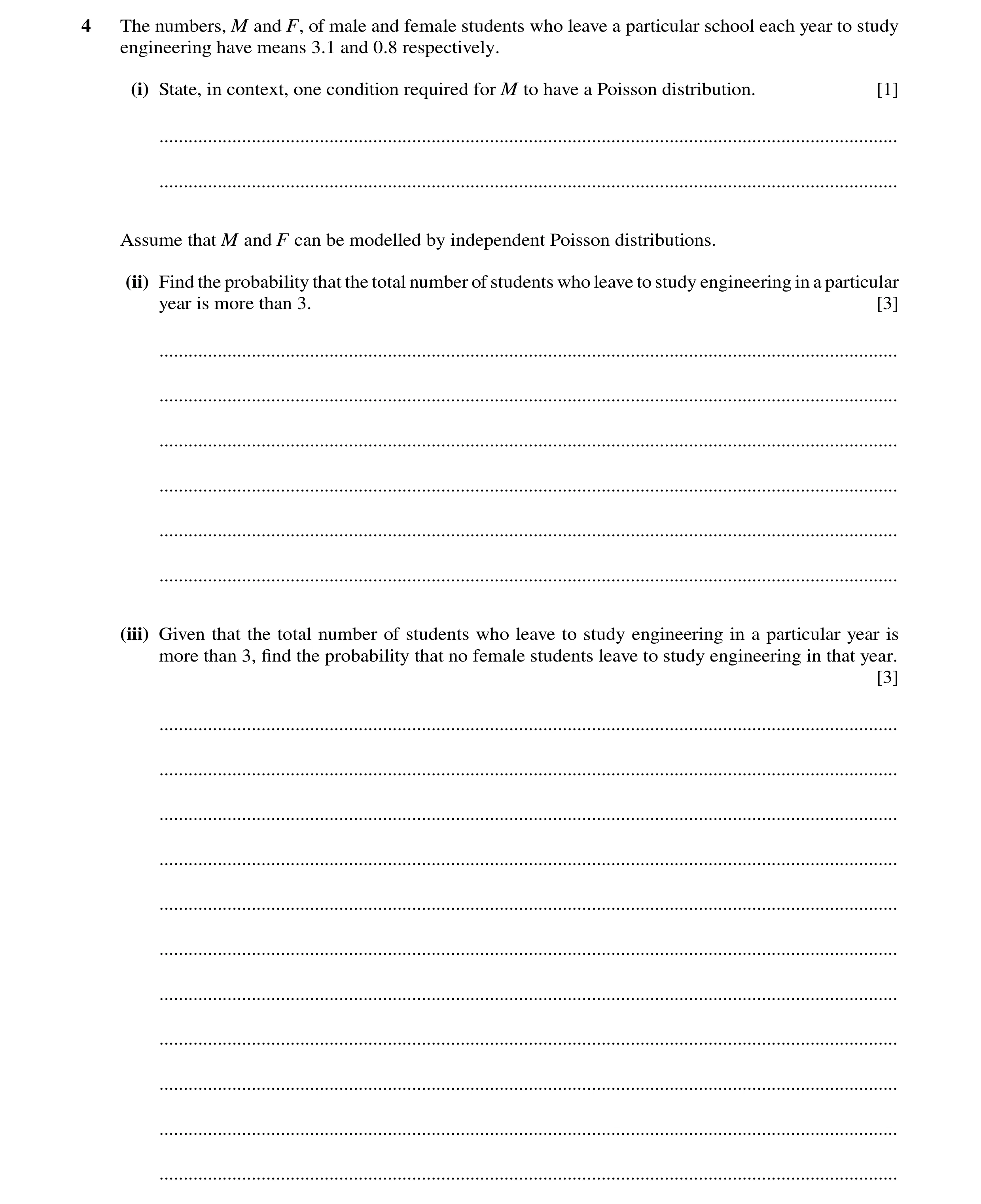
4 The numbers, M and F, of male and female students who leave a particular school each year to study engineering have means 3.1 and 0.8 respectively. (i) State, in context, one condition required for M to have a Poisson distribution. [1] … … Assume that M and F can be modelled by independent Poisson distributions. (ii) Find the probability that the total number of students who leave to study engineering in a particular year is more than 3. [3] … … … … … … (iii) Given that the total number of students who leave to study engineering in a particular year is more than 3, find the probability that no female students leave to study engineering in that year. [3] … … … … … … … … … … …
7 marks
Mark scheme: 4(i) No of males leaving (to do eng) each yr has const mean or Males leave (to do eng) indep of other males leaving (to do eng) or Males leave (to do eng) at random B1 1 4(ii) λ = 3.9 B1 1 – e–3.9(1 + 3.9 + 2 3 3.9 3.9 2! 3! + ) M1 Any λ. Allow one end error or extra term. 0.546753 or 0.547 (3 sf) A1 3 4(iii) P(F = 0 and M > 3) = 2 3 3.1 3.1 0.8 3.1 e 1 1 3.1 2! 3! e − − × − + + + (= 0.16857) M1 Attempt P(F = 0) × P(M > 3) allow one end error for P(M > 3) provided λ = 3.1 P(F=0 and M>3) P(M+F>3) "0.16857" "0.54675" M1 Attempted, allow any probability/their (ii) provided the answer is <1 = 0.308 (3 sf) A1 3
This question in 9709/73 May/June 2018
Q43 · Small drops of two liquids, A and B, are randomly and independently distributed in the air 9709/73 Oct/Nov 2018
4 Small drops of two liquids, A and B, are randomly and independently distributed in the air. The average numbers of drops of A and B per cubic centimetre of air are 0.25 and 0.36 respectively. (i) A sample of 10 cm3 of air is taken at random. Find the probability that the total number of drops of A and B in this sample is at least 4. [3] … … … … … … … … … … … … … … … … … … … … … … … (ii) A sample of 100 cm3 of air is taken at random. Use an approximating distribution to find the probability that the total number of drops of A and B in this sample is less than 60. [5] … … … … … … … … … … … … … … … … … … … … … … … … …
8 marks
Mark scheme: 4(i) λ = 10×0.25 + 10×0.36 ( = 6.1 ) B1 1 – e-6.1 (1 + 6.1 + 6.12 2 + 6.13!3 ) M1 1 – P(X ⩽ 3), any λ Allow one end error = 0.857 A1 Allow 0.858 3 4(ii) λ = 61 B1 ft Ft from (i) N(‘61’, ‘61’) M1 N with µ = λ, any λ. May be implied 59.5 − 61 (= –0.192) M1 Standardise with their mean and variance '61' Allow no or wrong cc. not 61/100 Φ(‘–0.192’) = 1 – Φ(‘0.192’) M1 Correct area consistent with their working = 0.424 A1 5
This question in 9709/73 Oct/Nov 2018
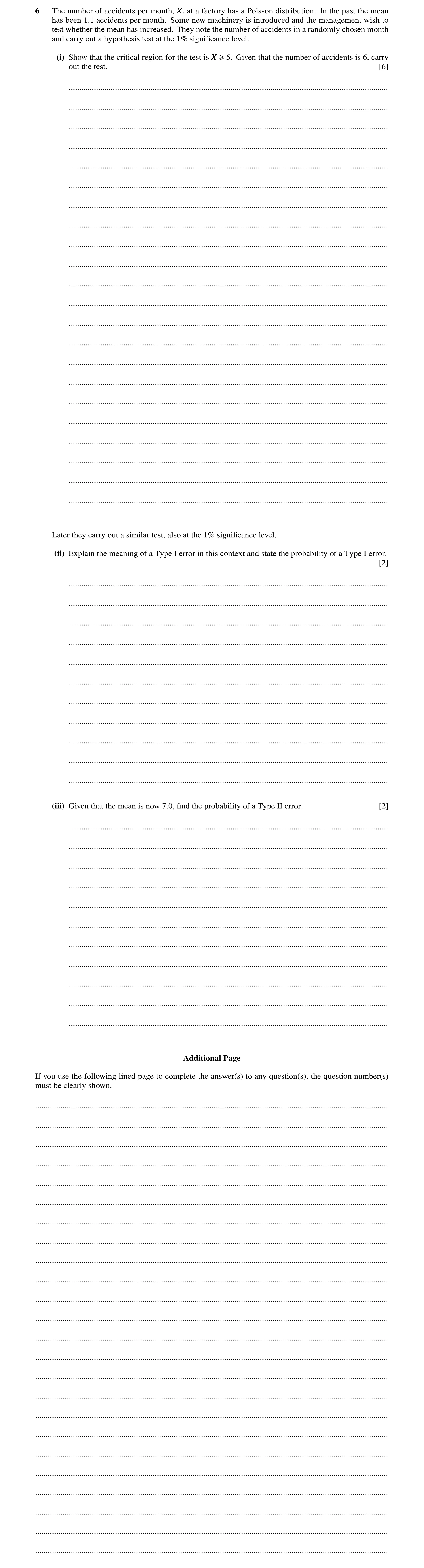
Q44 · The number of accidents per month, X, at a factory has a Poisson distribution 9709/72 Oct/Nov 2019
6 The number of accidents per month, X, at a factory has a Poisson distribution. In the past the mean has been 1.1 accidents per month. Some new machinery is introduced and the management wish to test whether the mean has increased. They note the number of accidents in a randomly chosen month and carry out a hypothesis test at the 1% significance level. (i) Show that the critical region for the test is X ≥5. Given that the number of accidents is 6, carry out the test. [6] … … … … … … … … … … … … … … … … … … … … … … Later they carry out a similar test, also at the 1% significance level. (ii) Explain the meaning of a Type I error in this context and state the probability of a Type I error. [2] … … … … … … … … … … … (iii) Given that the mean is now 7.0, find the probability of a Type II error. [2] … … … … … … … … … … … Additional Page If you use the following lined page to complete the answer(s) to any question(s), the question number(s) must be clearly shown. … … … … … … … … … … … … … … … … … … … … … … … …
10 marks
Mark scheme: 6(i) H0: Pop mean (or λ or µ) is 1.1 H1: Pop mean (or λ or µ) is more than 1.1 P(X ⩾ 4) = 1 −e–1.1 2 3 1.1 1.1 1 1.1 2 3! + + + M1 Correct expression for either P(X ⩾ 4) or P(X ⩾ 5) 0.0257 A1 Correct value of either P(X ⩾ 4) or P(X ⩾ 5) ( ) 4 1.1 1.1 P 0.0257 e 0.00544 4! 5 X − = − × = . B1 B1 for the other value (Note use of P(X < 4) = 0.9743 and P(X < 5) = 0.99456 can score only if comparison with 0.99 seen) 0.00544 < 0.01 < 0.0257 M1 OE stated (valid comparison) There is evidence mean has increased B1 SC P(X ⩾ 6) = 0.000968 M1A1 Conclusion B1 6 6(ii) Concluding mean has increased when it has not B1 In context ‘0.00544’ B1FT FT their P(X ⩾ 5), dep < 0.01 2 6(iii) 2 3 4 7.0 7 7 7 e 1 7 2 3! 4! − + + + + M1 Correct expression for P(X ⩽ 4 | λ = 7.0) 0.173 (3 sf) A1 2
This question in 9709/72 Oct/Nov 2019
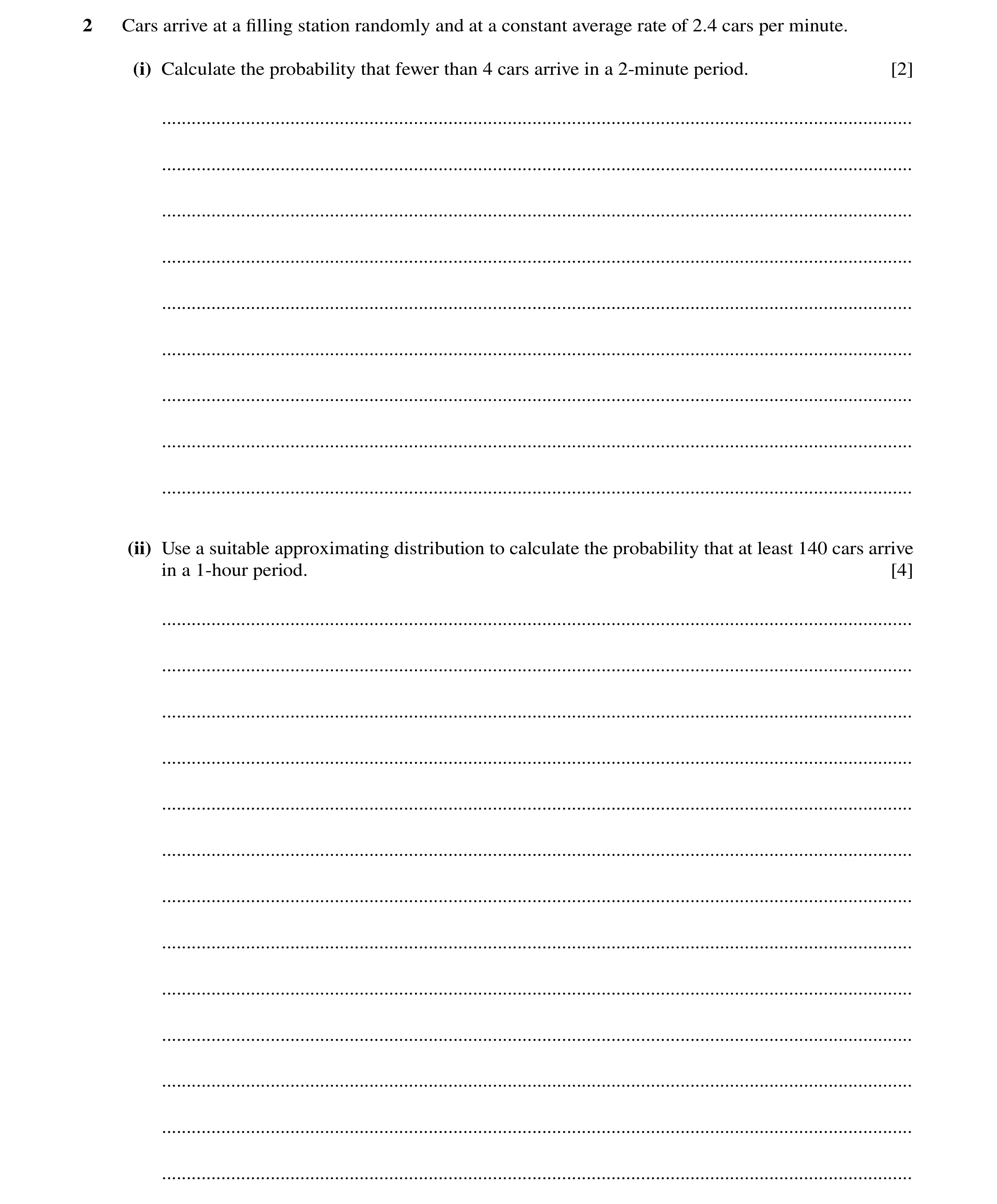
Q45 · Cars arrive at a filling station randomly and at a constant average rate of 2.4 cars per… 9709/73 Oct/Nov 2019
2 Cars arrive at a filling station randomly and at a constant average rate of 2.4 cars per minute. (i) Calculate the probability that fewer than 4 cars arrive in a 2-minute period. [2] … … … … … … … … … (ii) Use a suitable approximating distribution to calculate the probability that at least 140 cars arrive in a 1-hour period. [4] … … … … … … … … … … … … …
6 marks
Mark scheme: 2(i) 2 2.4 4.8 λ = × = 2 3 4.8 4.8 4.8 e 1 4 2 3! − + + + M1 Any λ 0.294 (3 sf) A1 2 2(ii) ( ) ( ) 60 2.4 144 λ = × = N(‘144’, ‘144’) M1 N and σ2=µ SOI ( ) 139.5 '144' 0.375 '144' − = − M1 Allow with no continuity correction φ(‘0.375’) M1 Correct area consistent with their working 0.646 (3 sf) A1 4
This question in 9709/73 Oct/Nov 2019
 1 / 30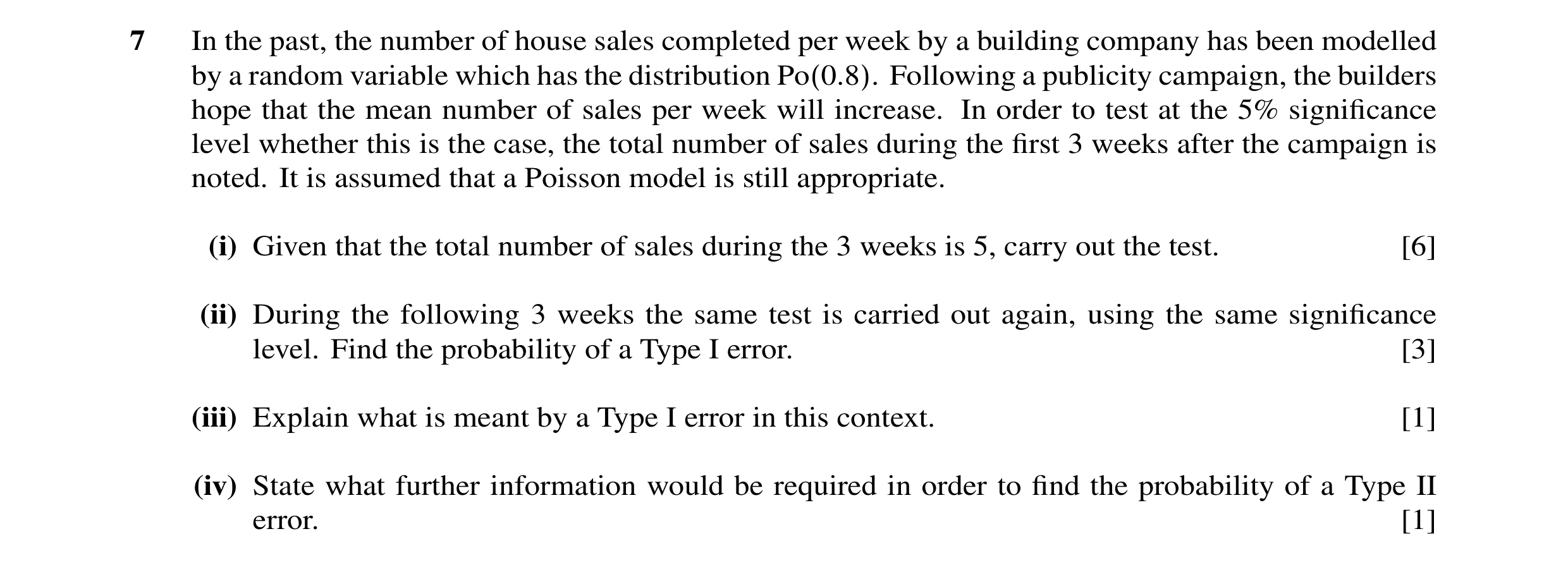
![Question 7: The random variable X has the distribution Po(1.3). The random variable Y is defined by Y = 2X. (i) Find the mean and variance of Y. [3] (ii…](https://img.pastlit.com/crops/c4bb05bb-805a-4cb5-917a-c4fb134efbc8/q1.webp)
 2 / 30
![Question 9: The random variable X has the distribution Po(1.3). The random variable Y is defined by Y = 2X. (i) Find the mean and variance of Y. [3] (ii…](https://img.pastlit.com/crops/1ef811a5-7ce8-4f88-a2f6-b11082bea171/q1.webp)
![Question 12: A random variable X has the distribution Po(3.2). (i) A random value of X is found. (a) Find P(X ≥3). [2] (b) Find the probability that X =…](https://img.pastlit.com/crops/9914268f-74de-4386-a000-2961578bb88e/q5.webp) 3 / 30
3 / 30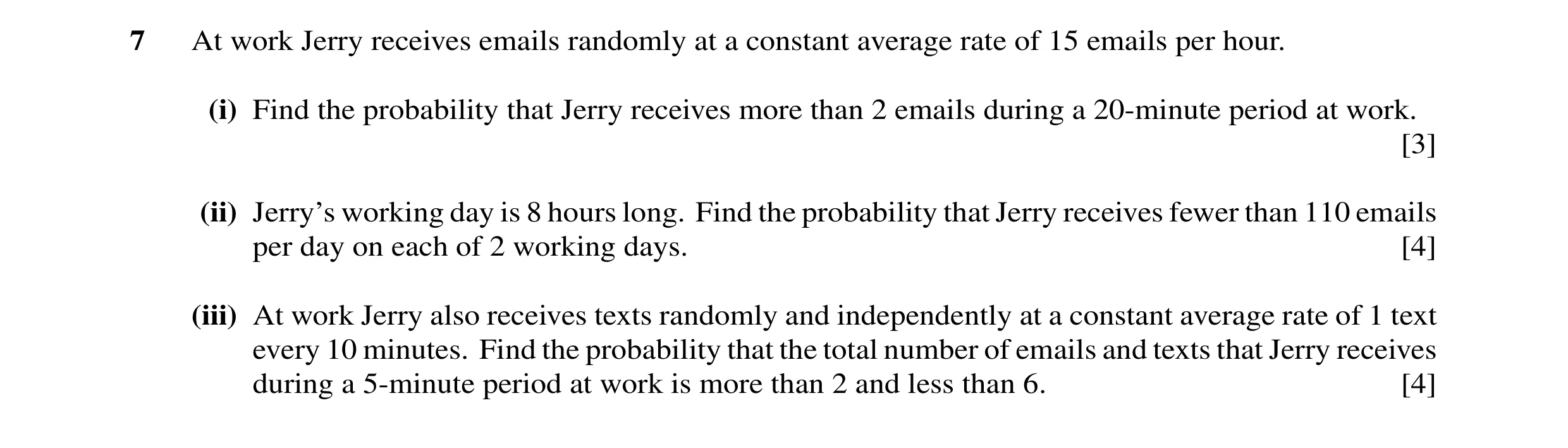

 4 / 30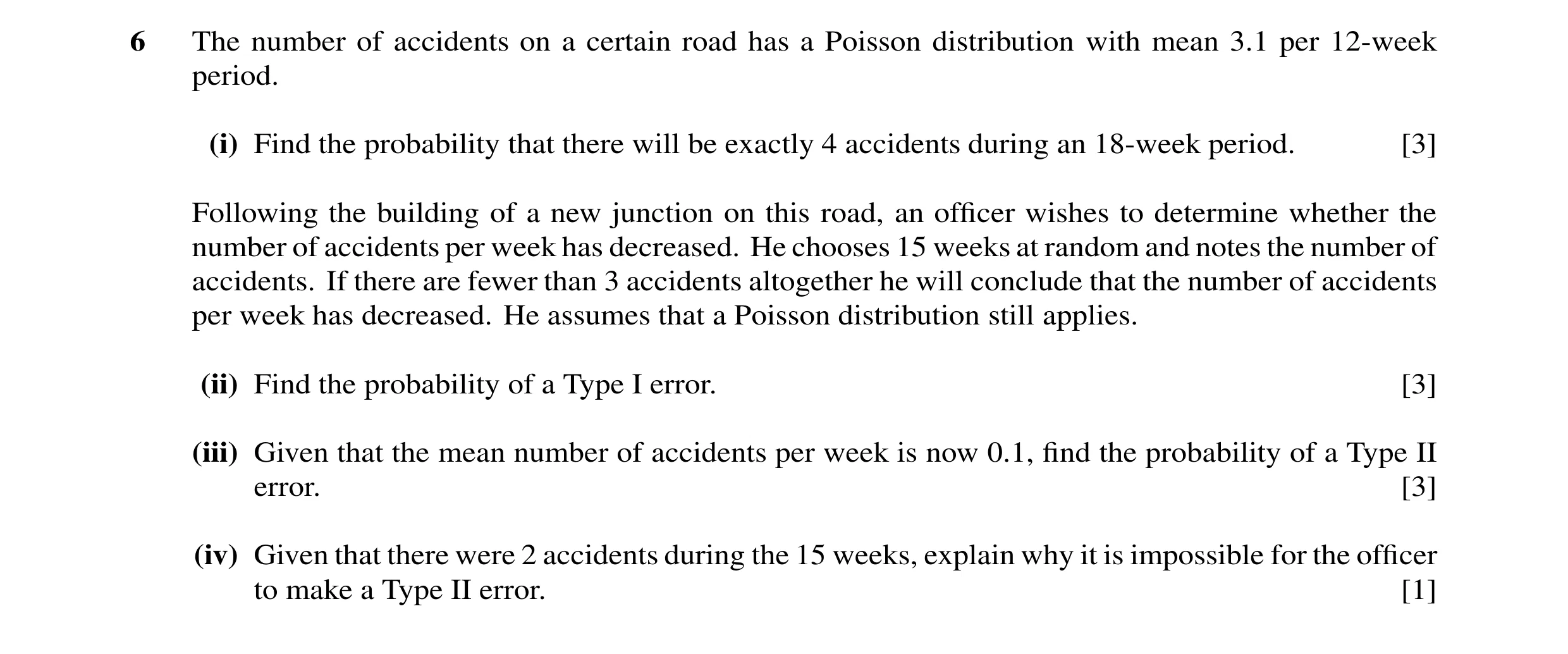
 5 / 30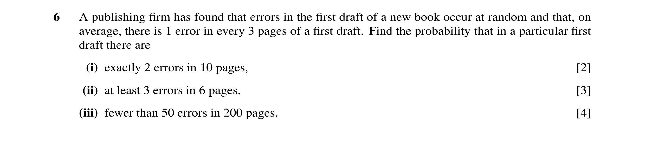


 6 / 30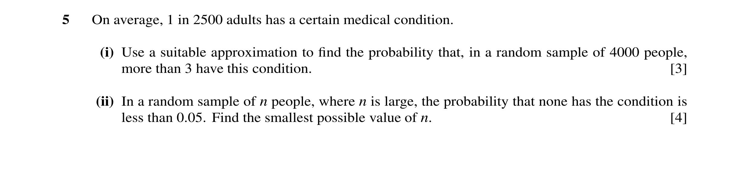
 7 / 30
 8 / 30
 9 / 30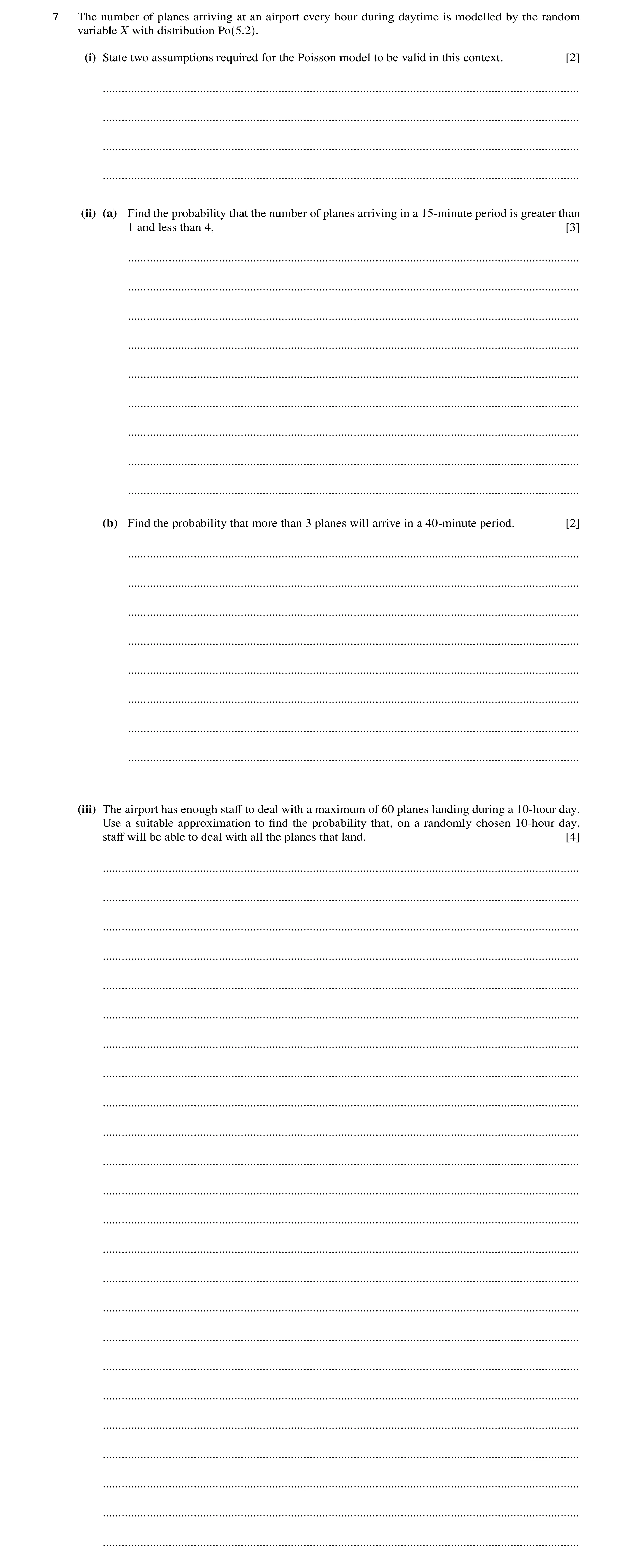
 12 / 30
 24 / 30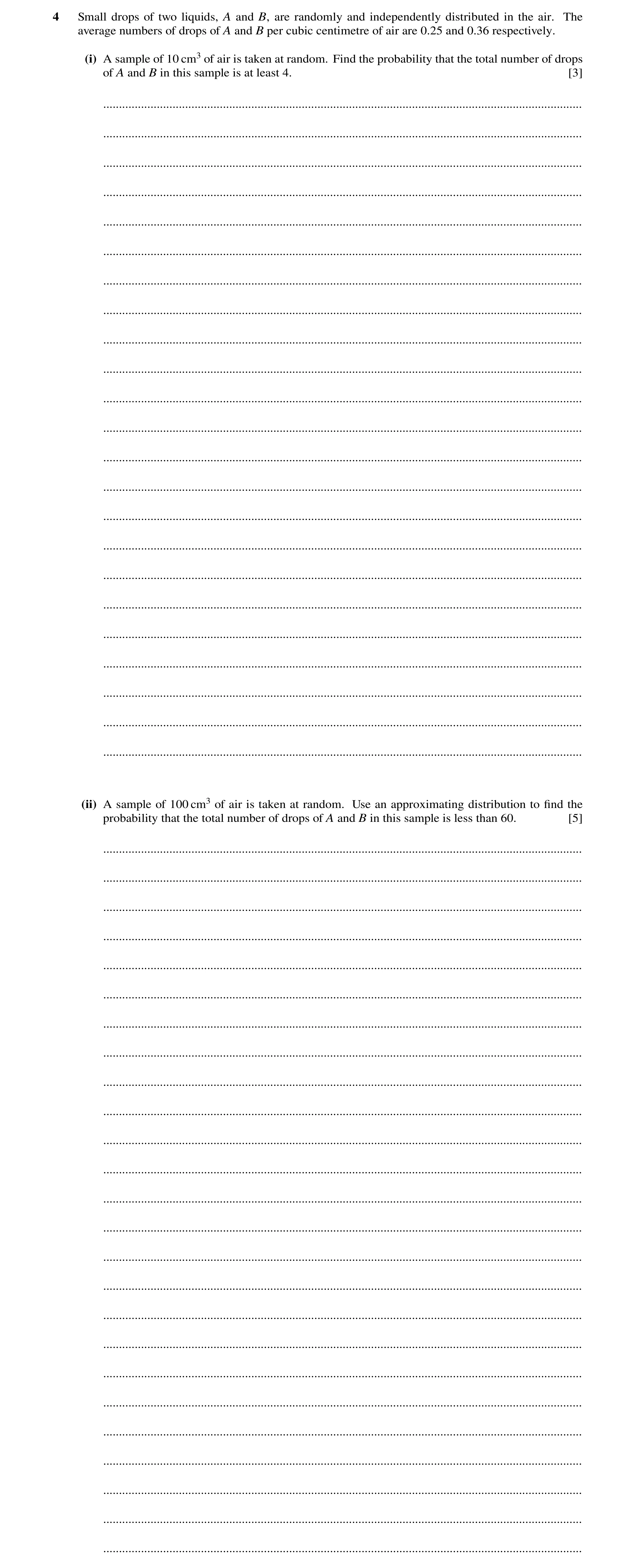
 30 / 30
 10
10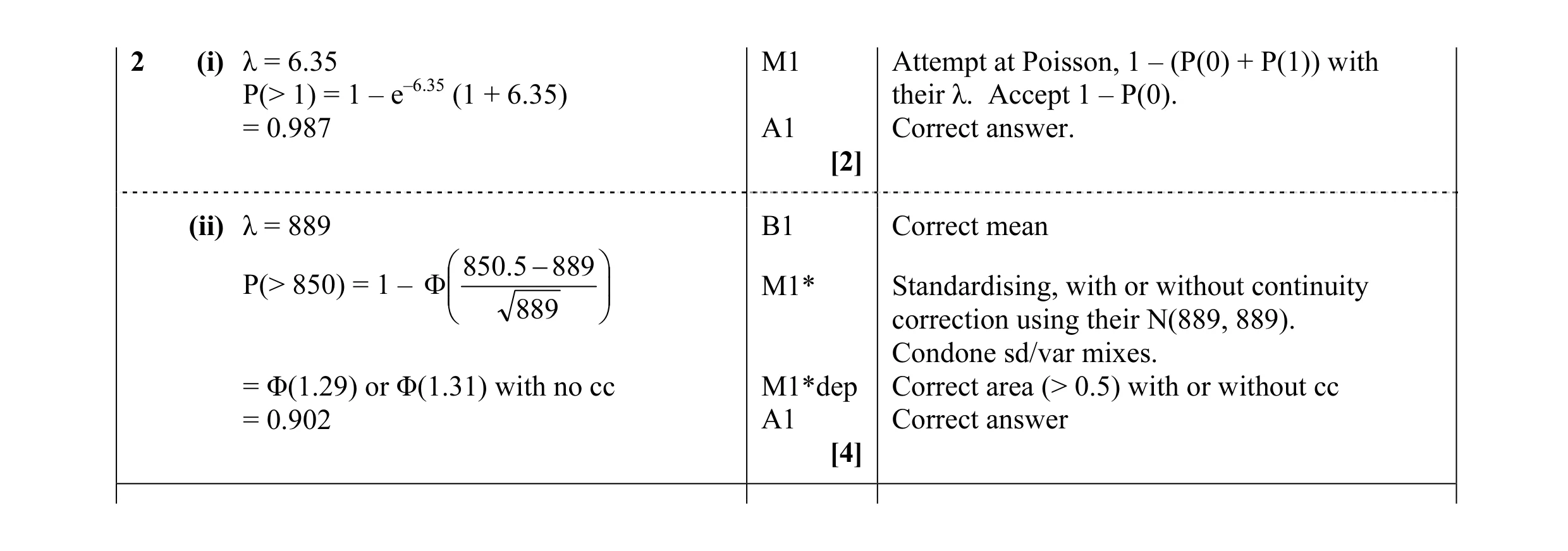 6
6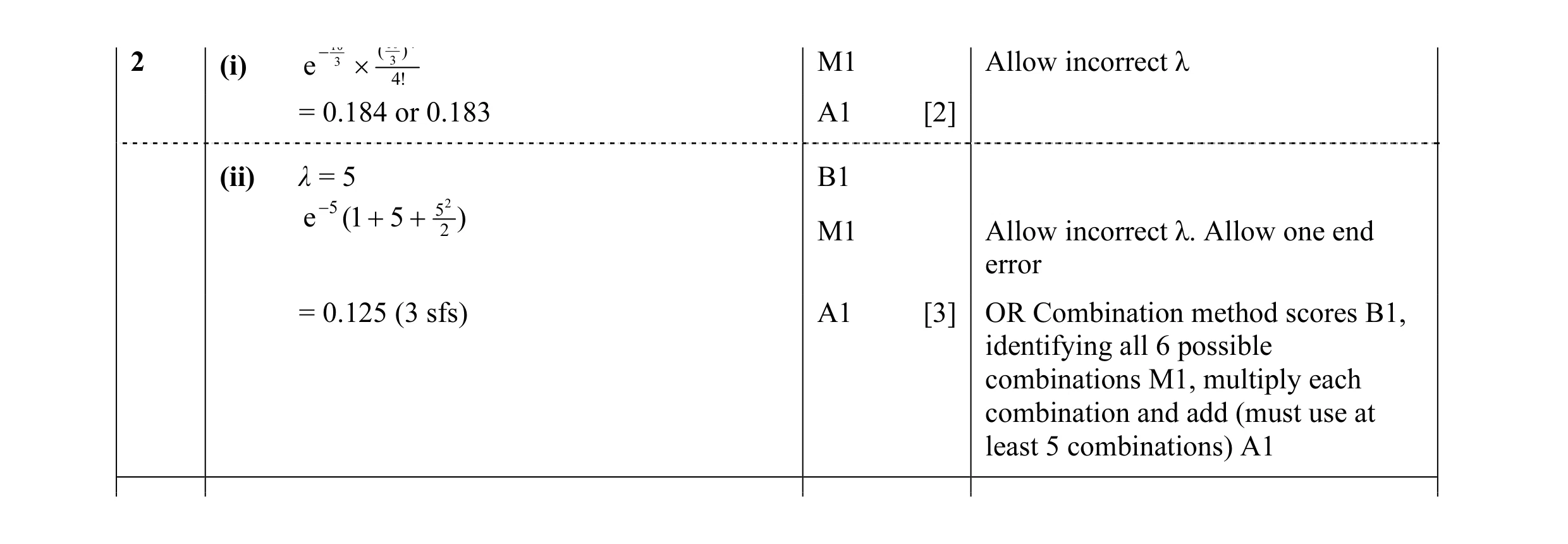 5
5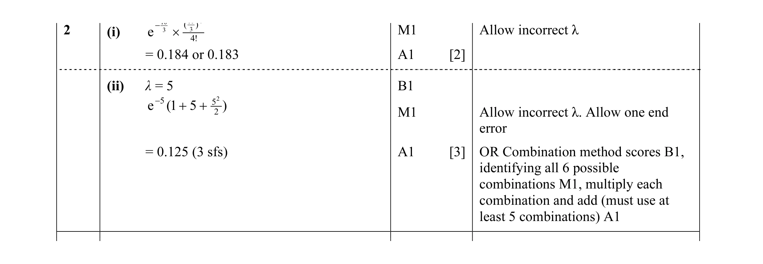 5
5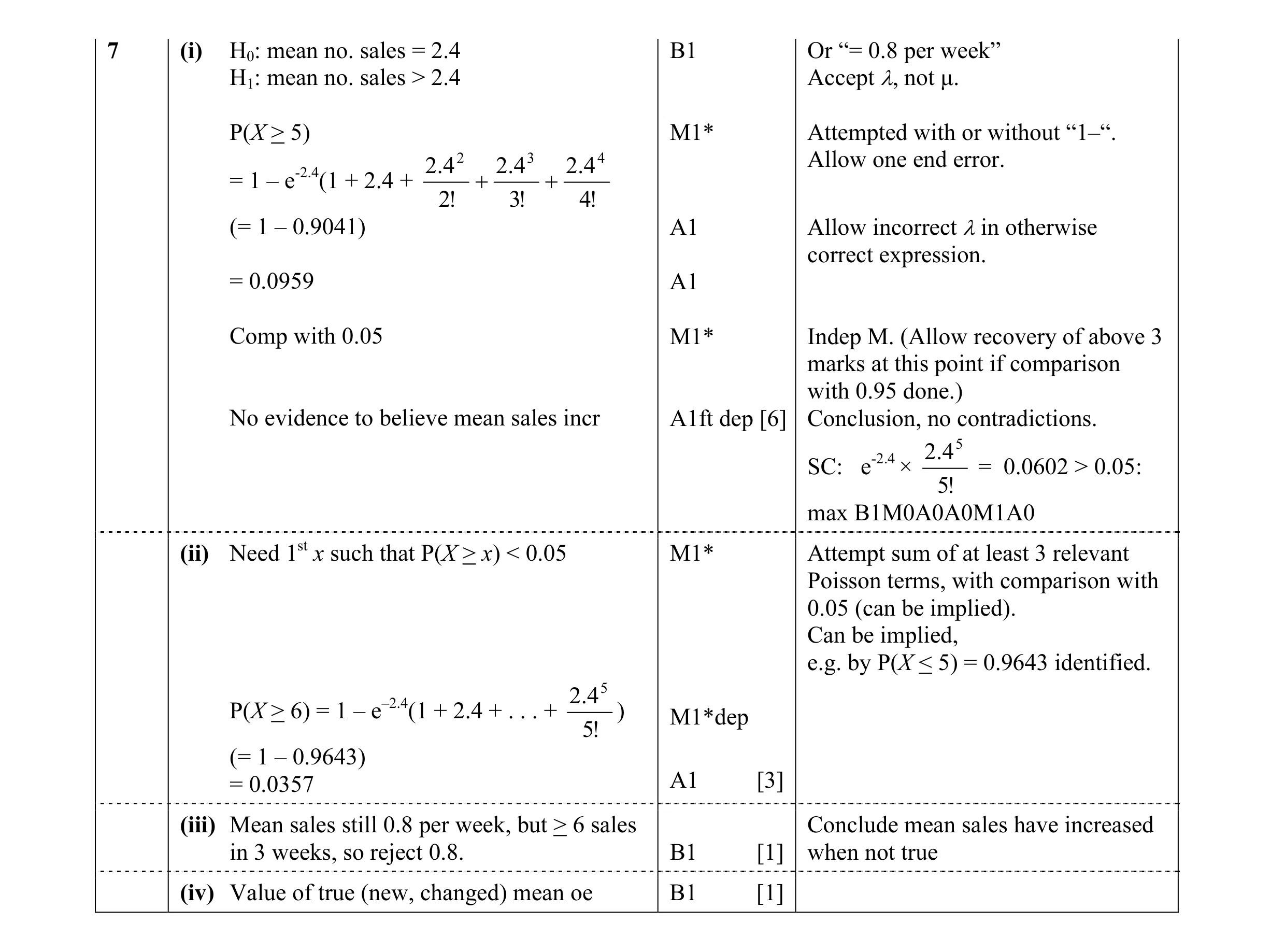 11
11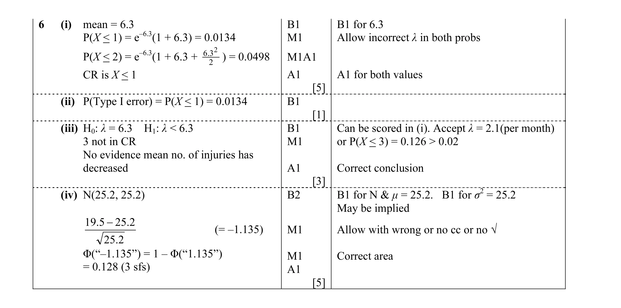 14
14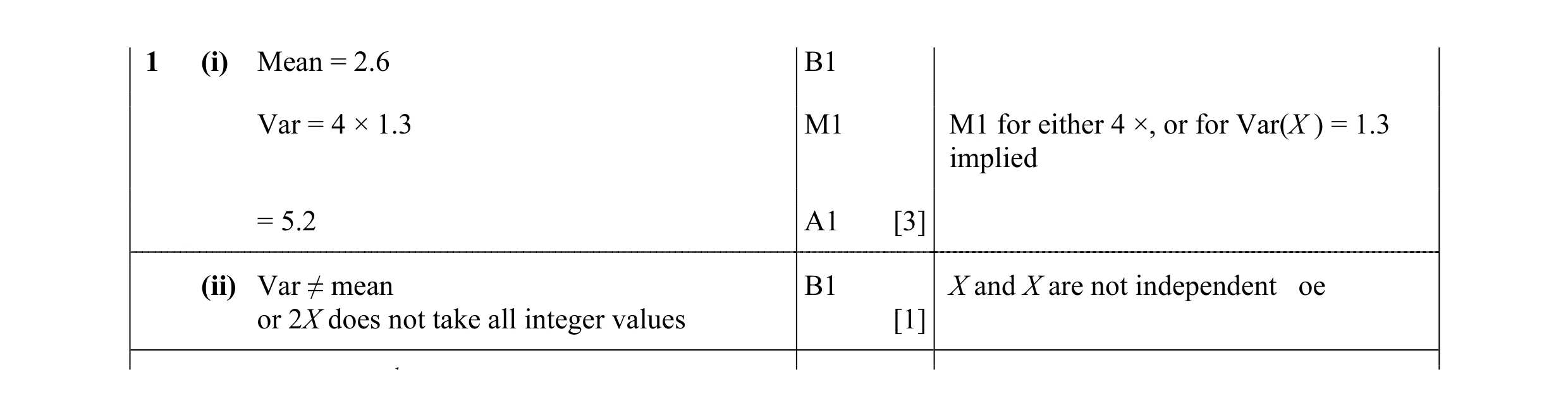 4
4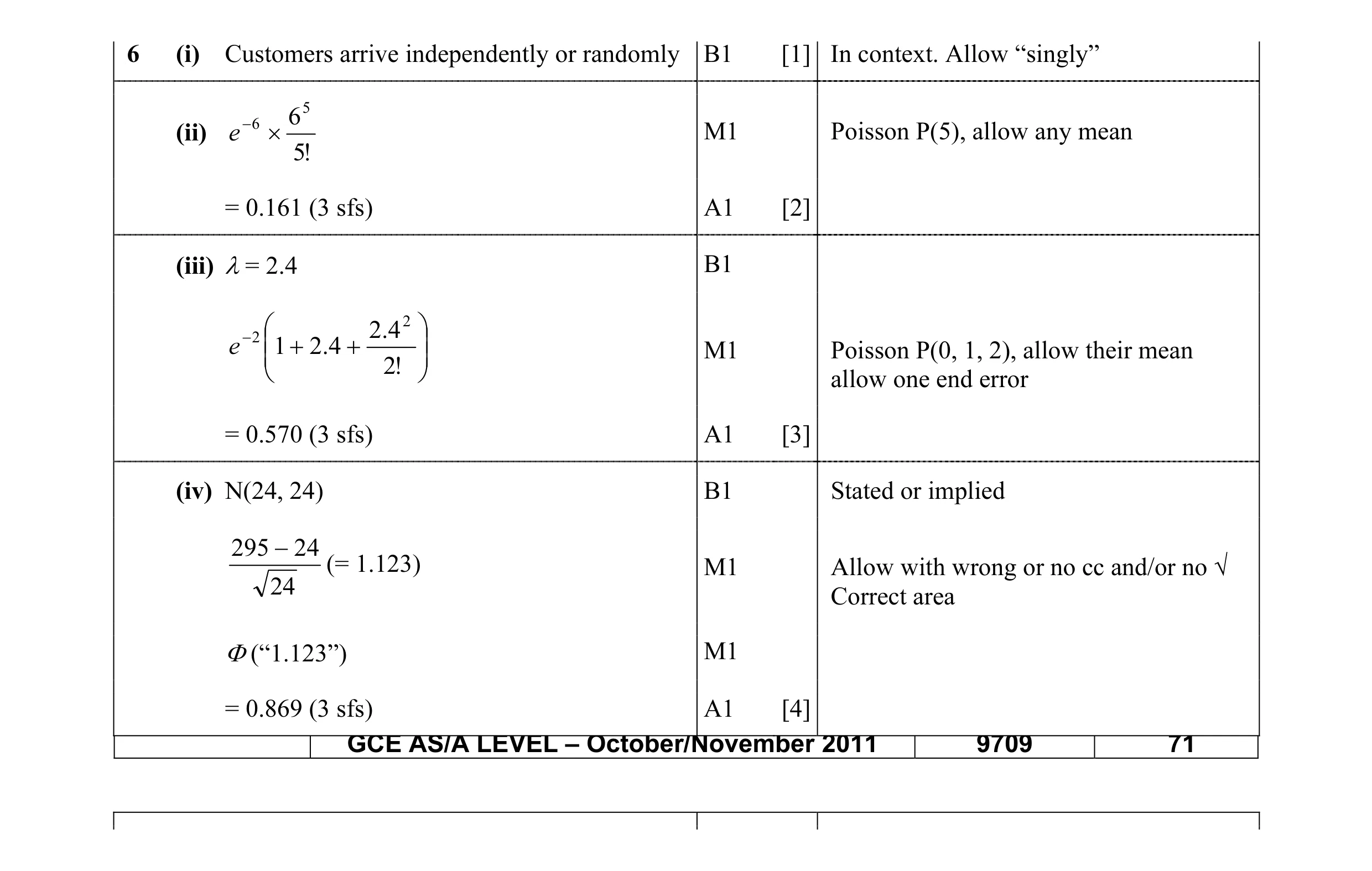 10
10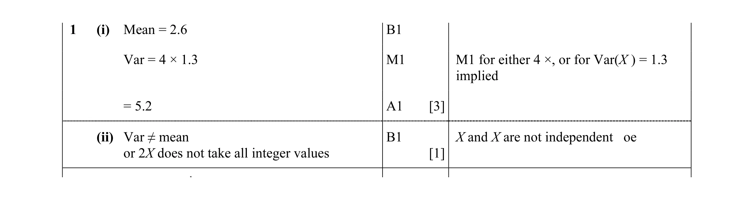 4
4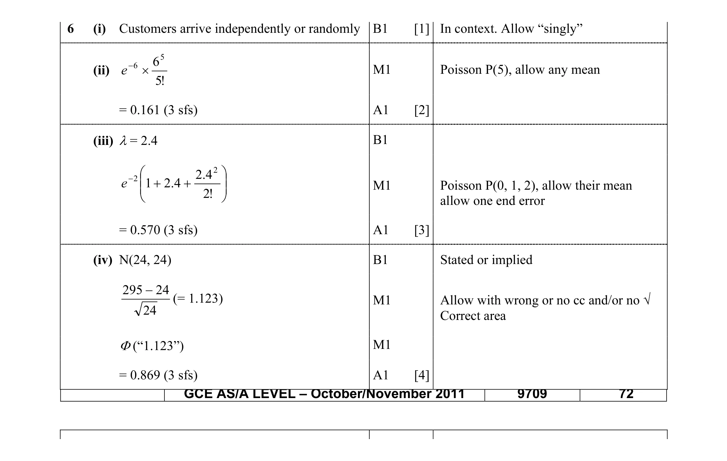 10
10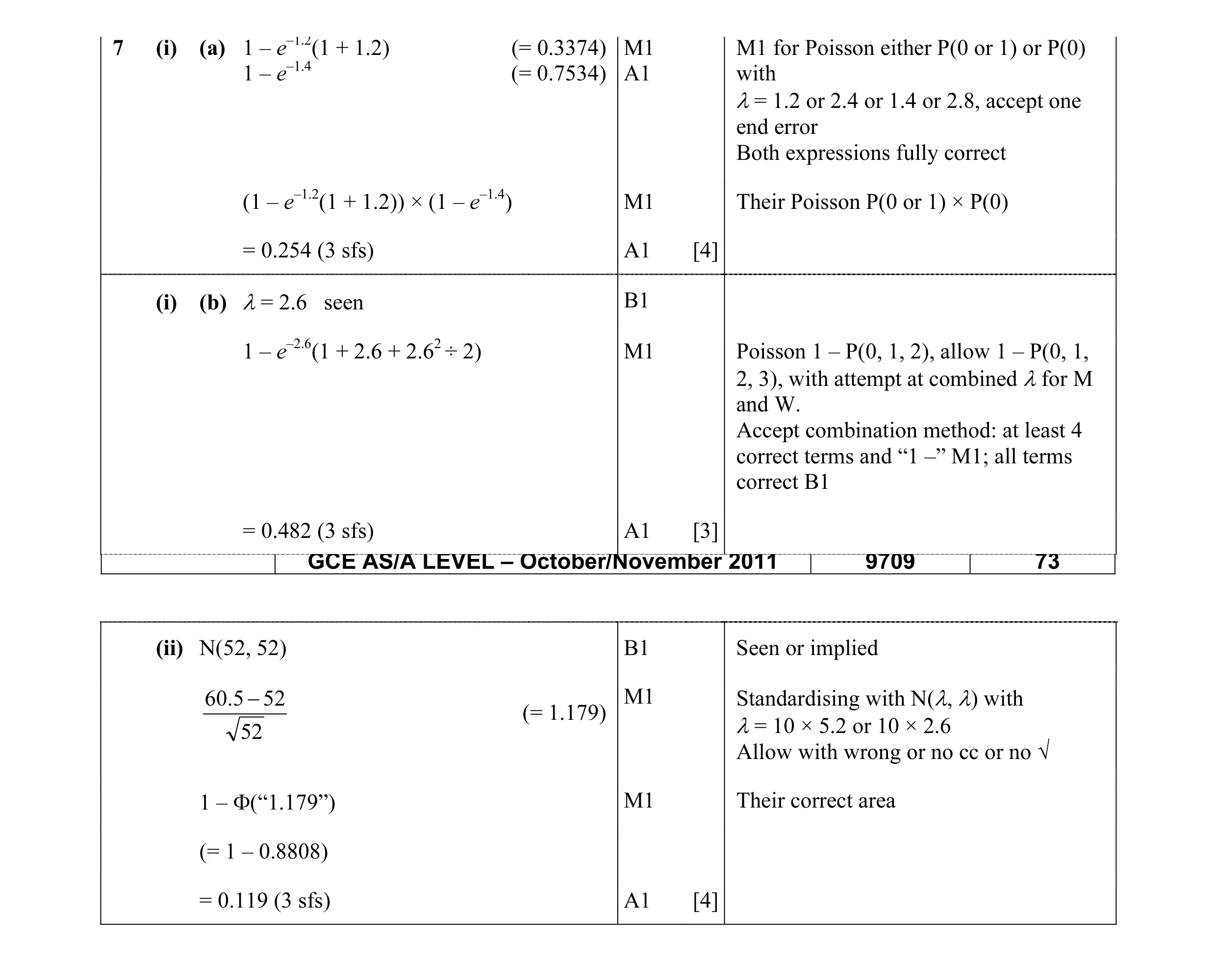 11
11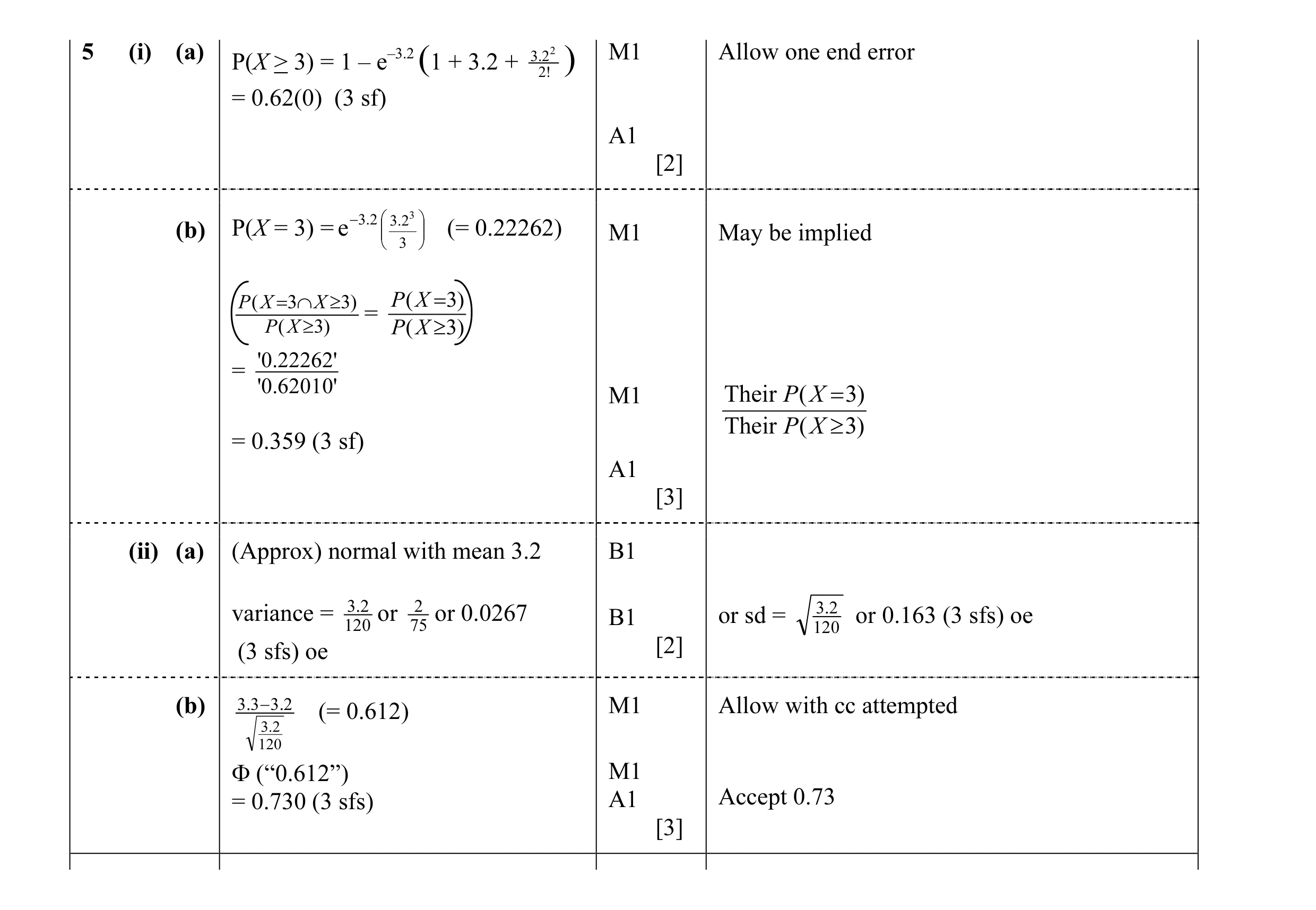 10
10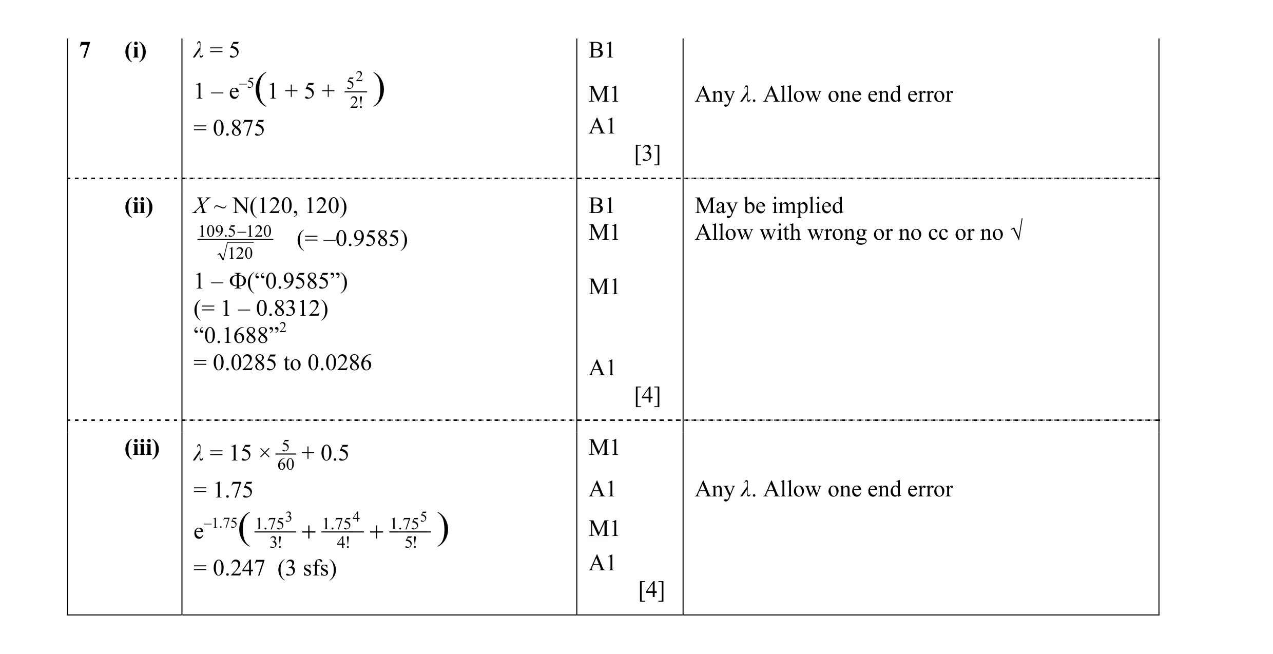 11
11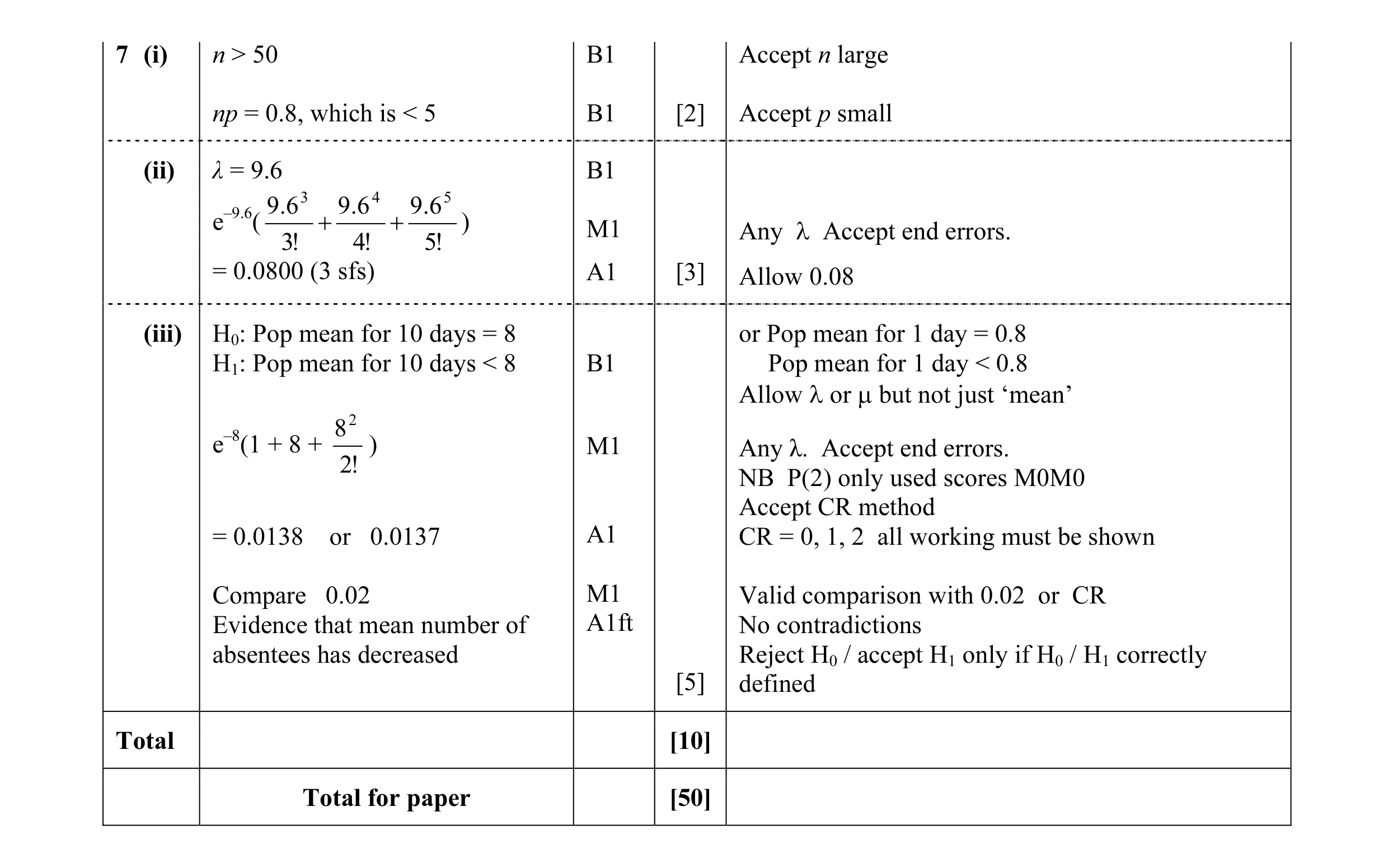 10
10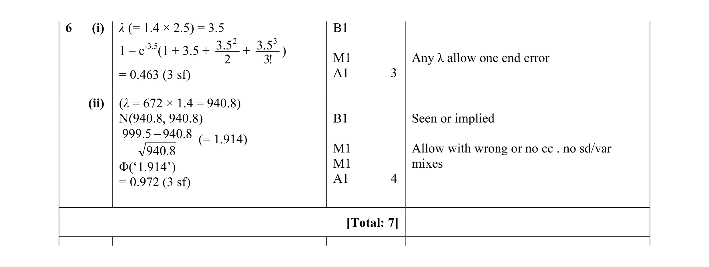 7
7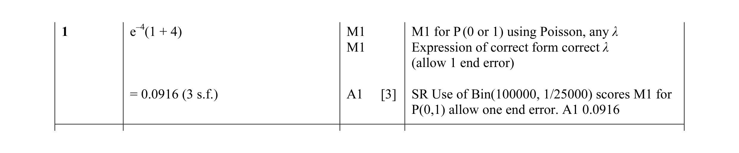 3
3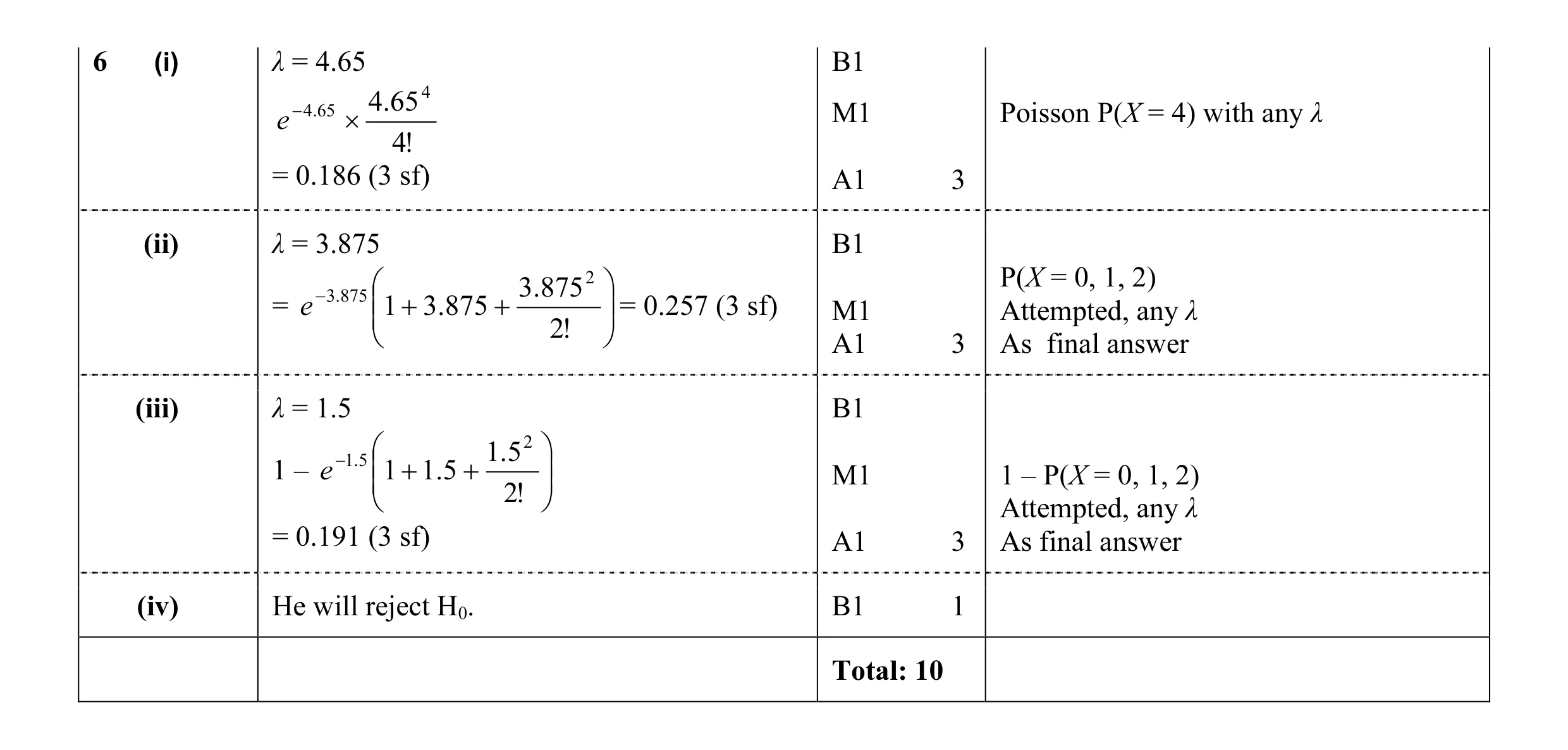 10
10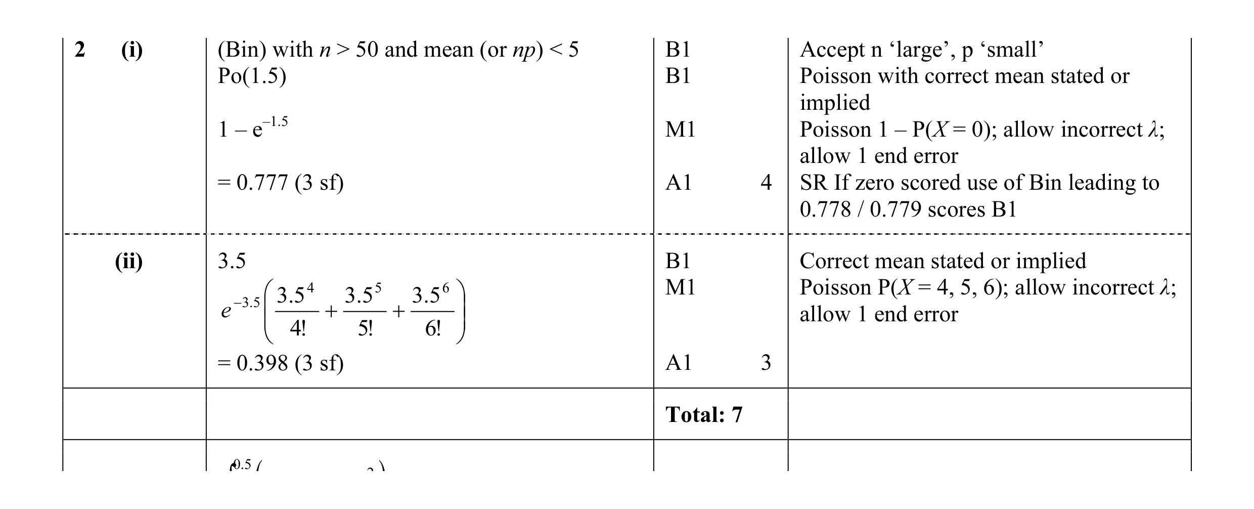 7
7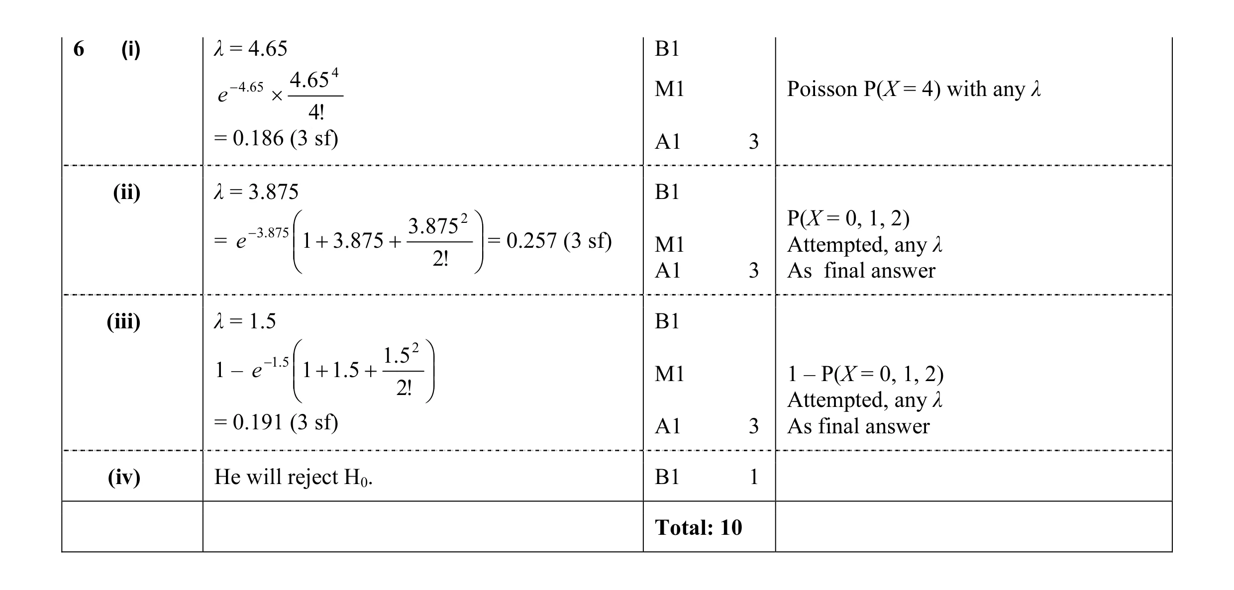 10
10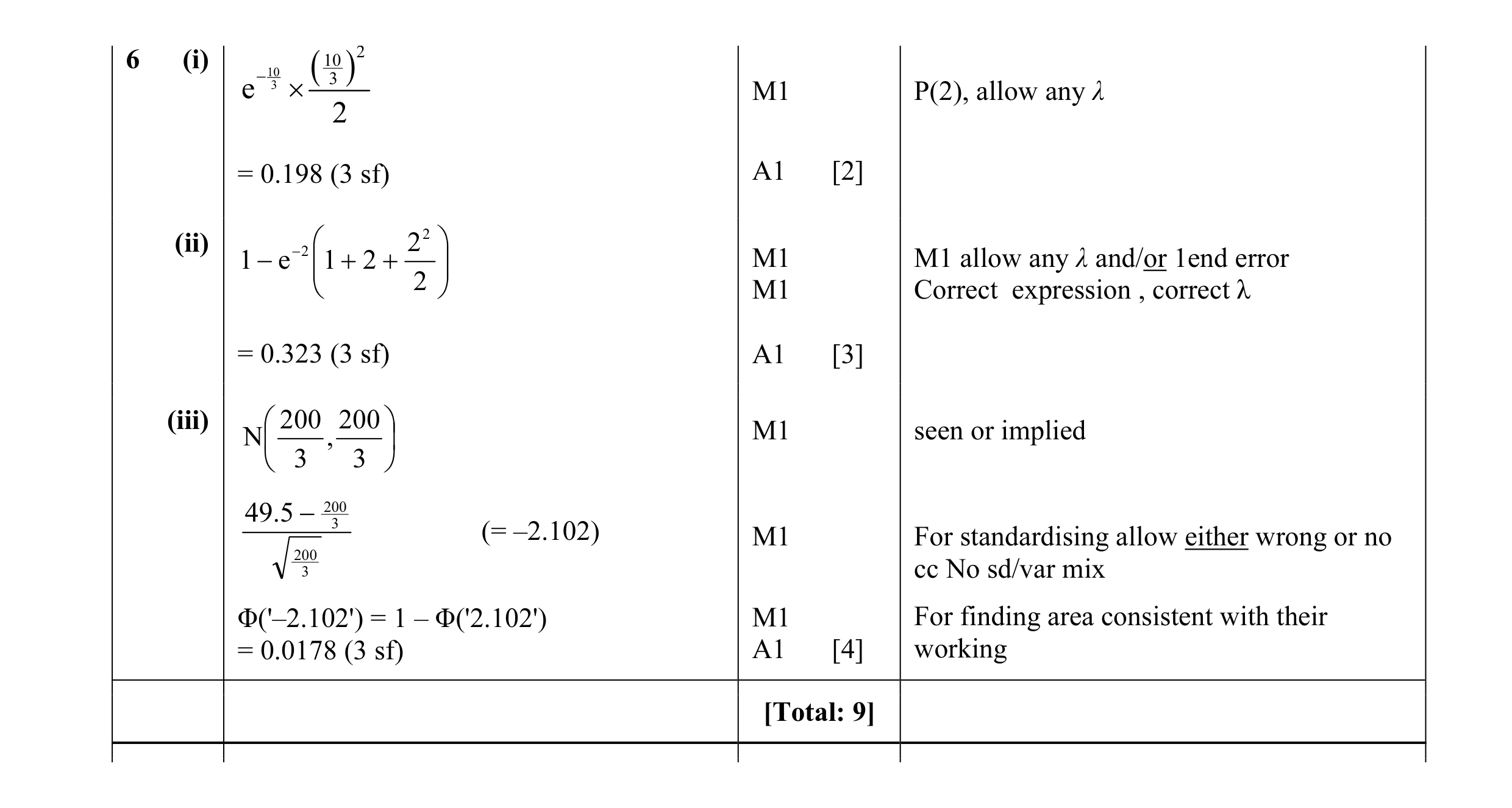 9
9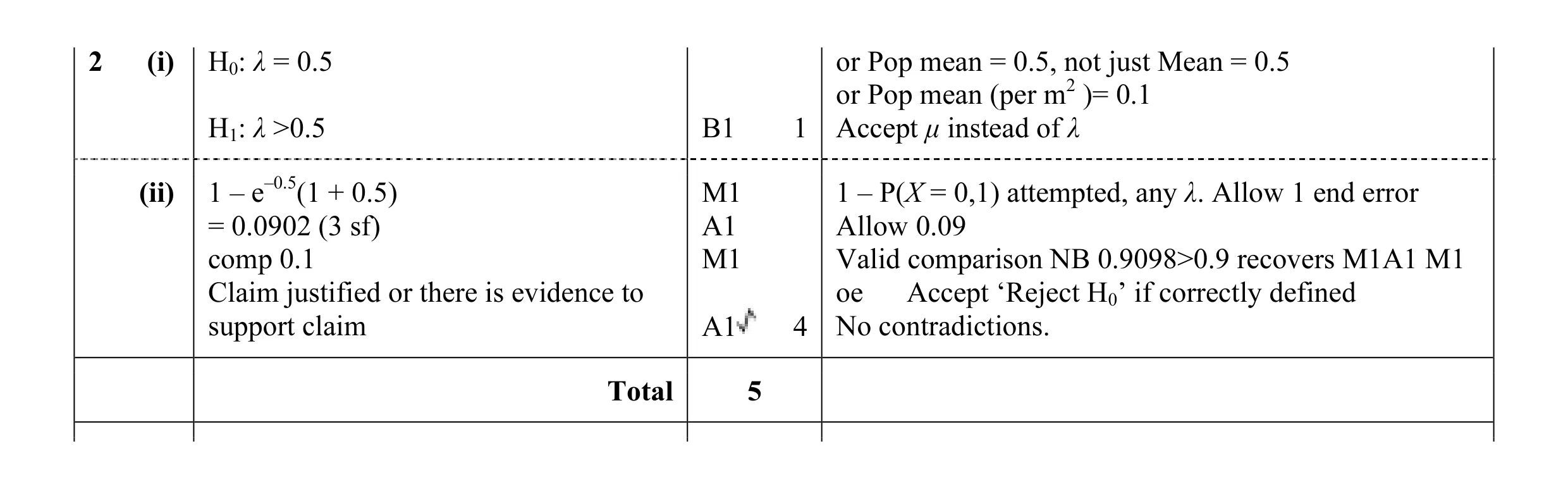 5
5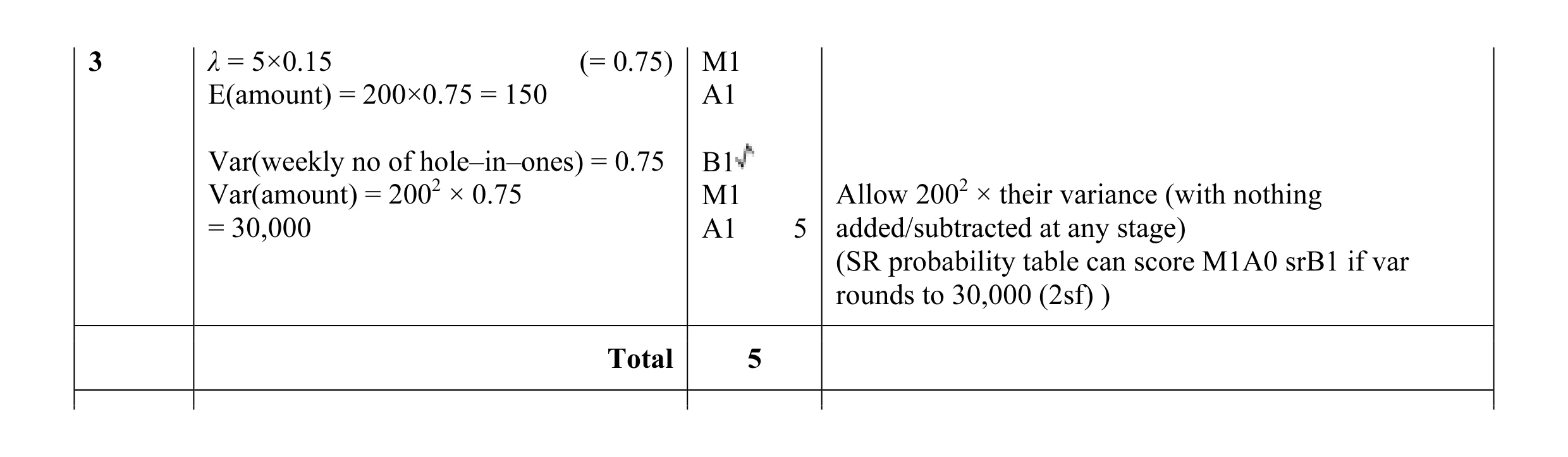 5
5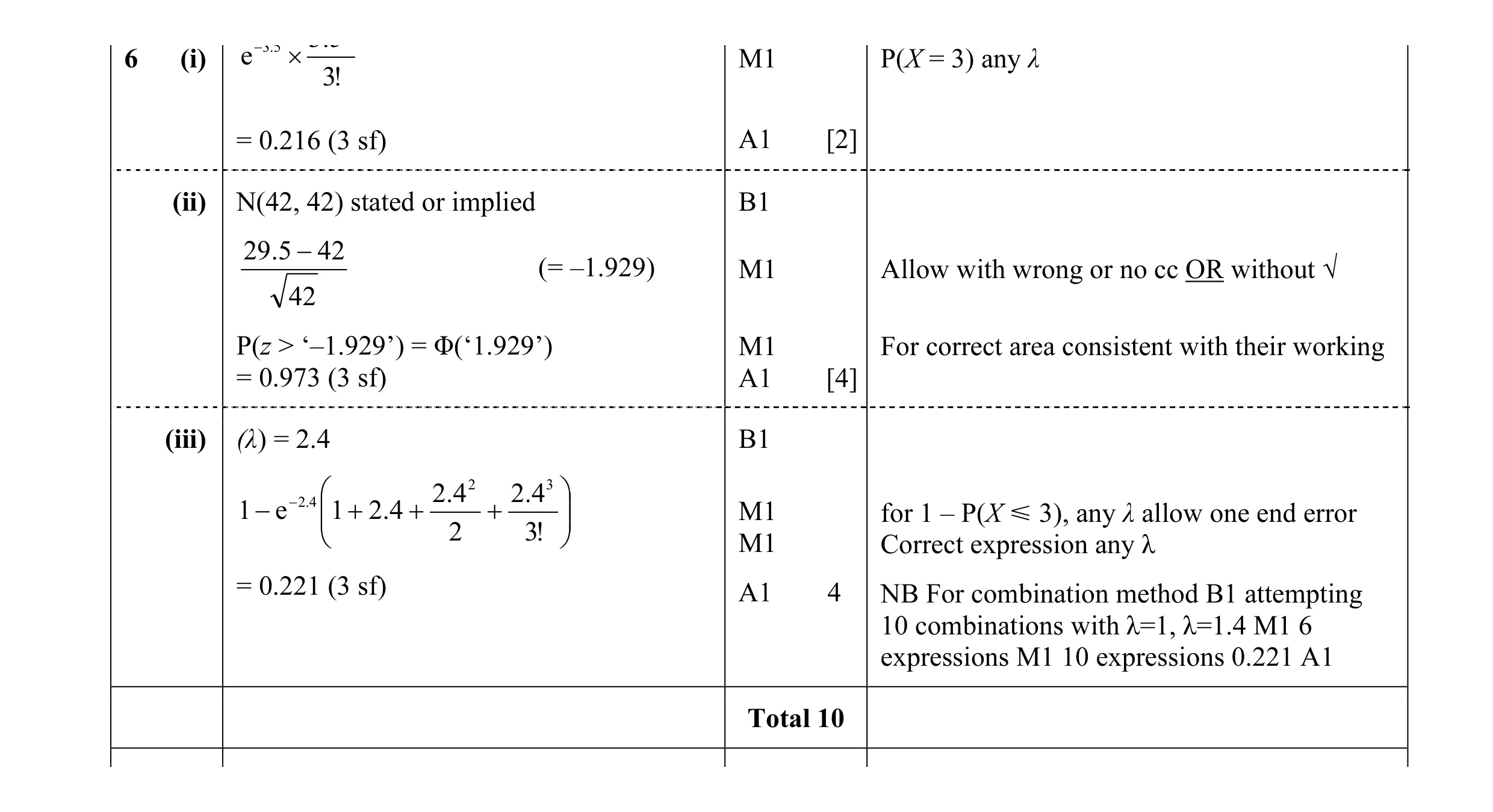 10
10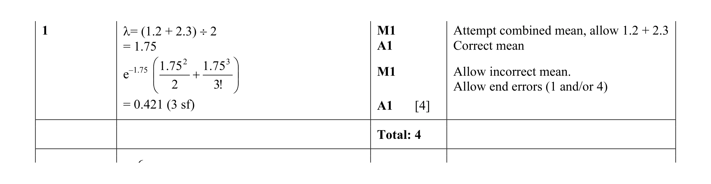 4
4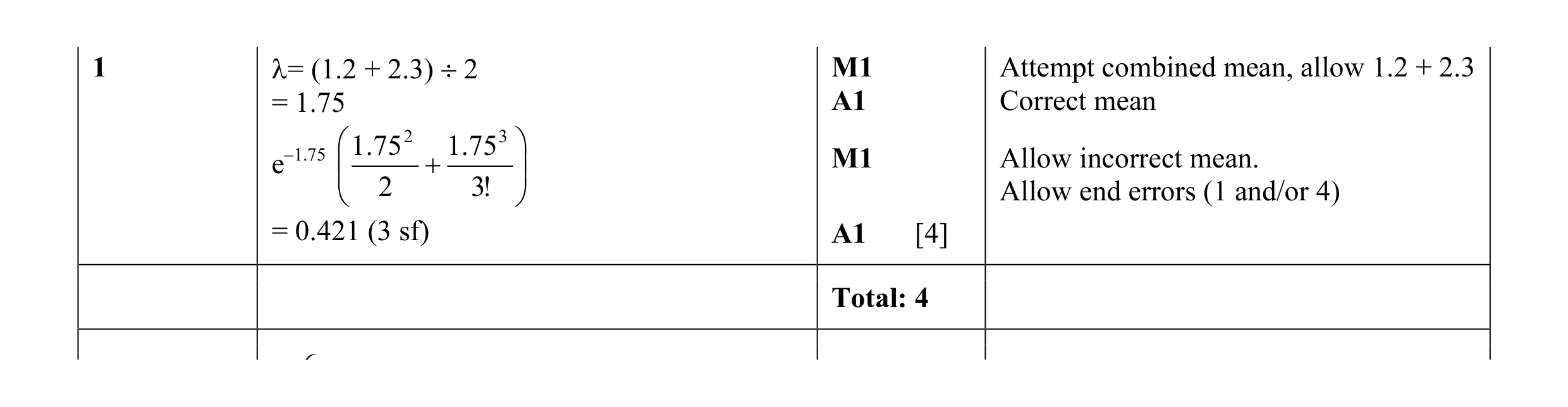 4
4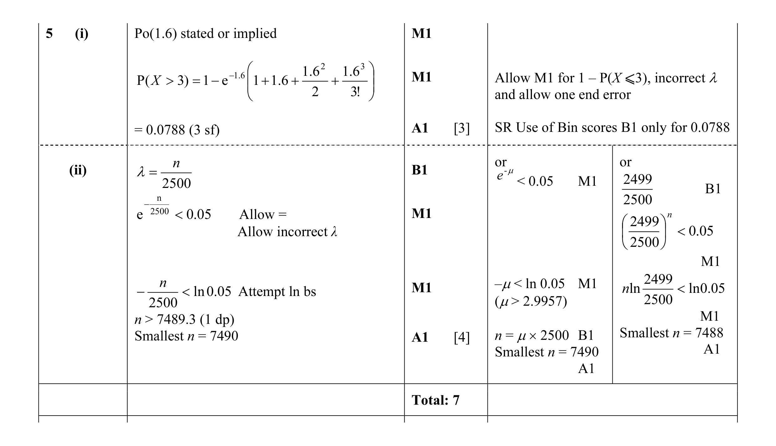 7
7 9
9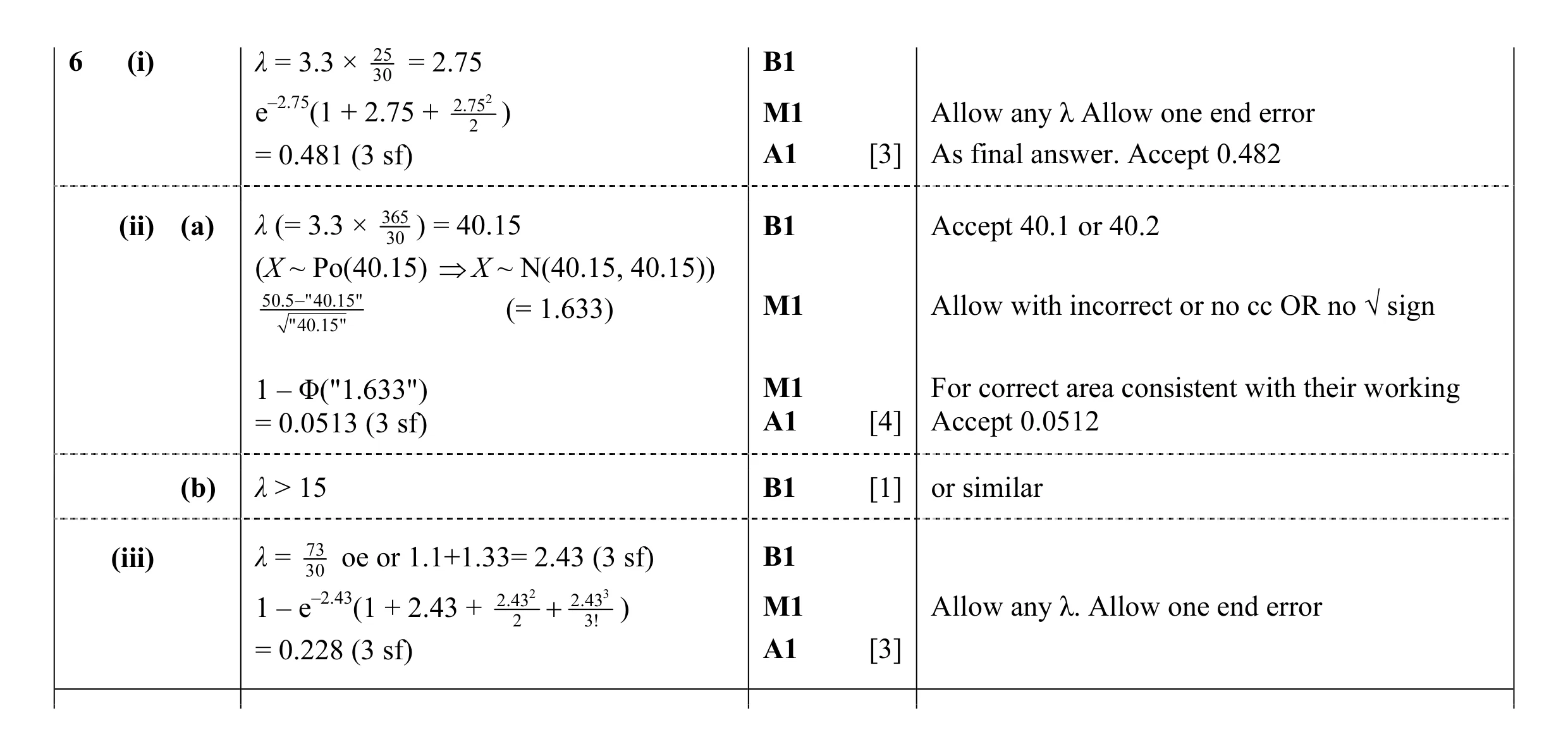 11
11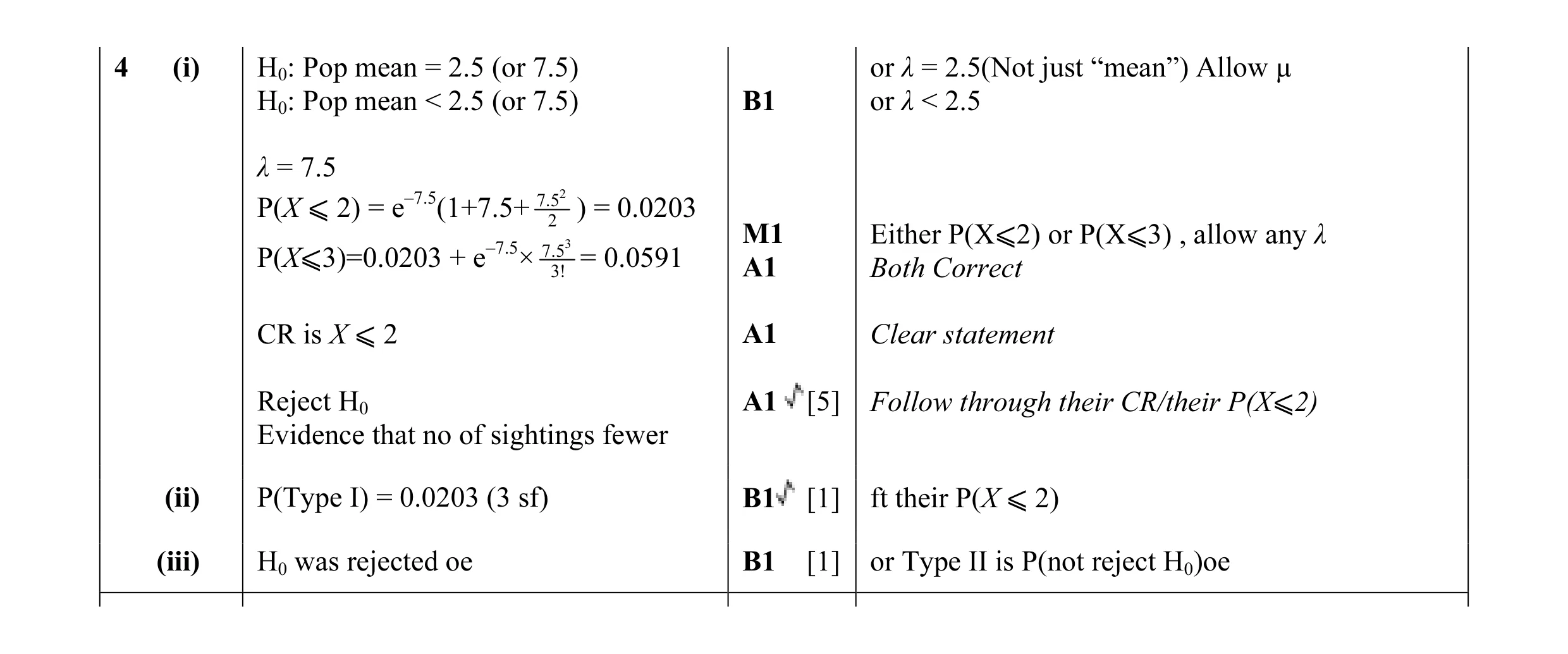 7
7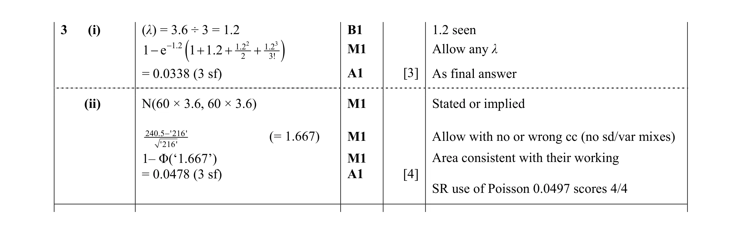 7
7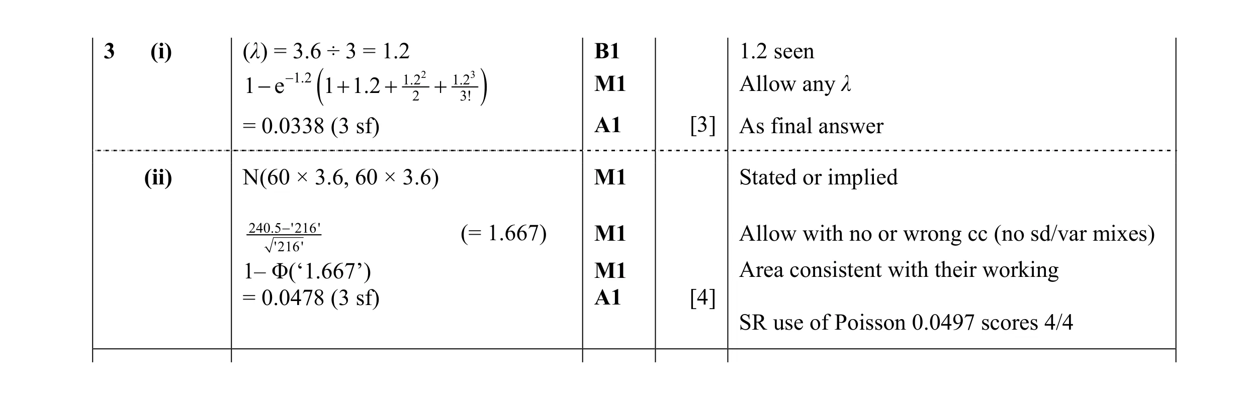 7
7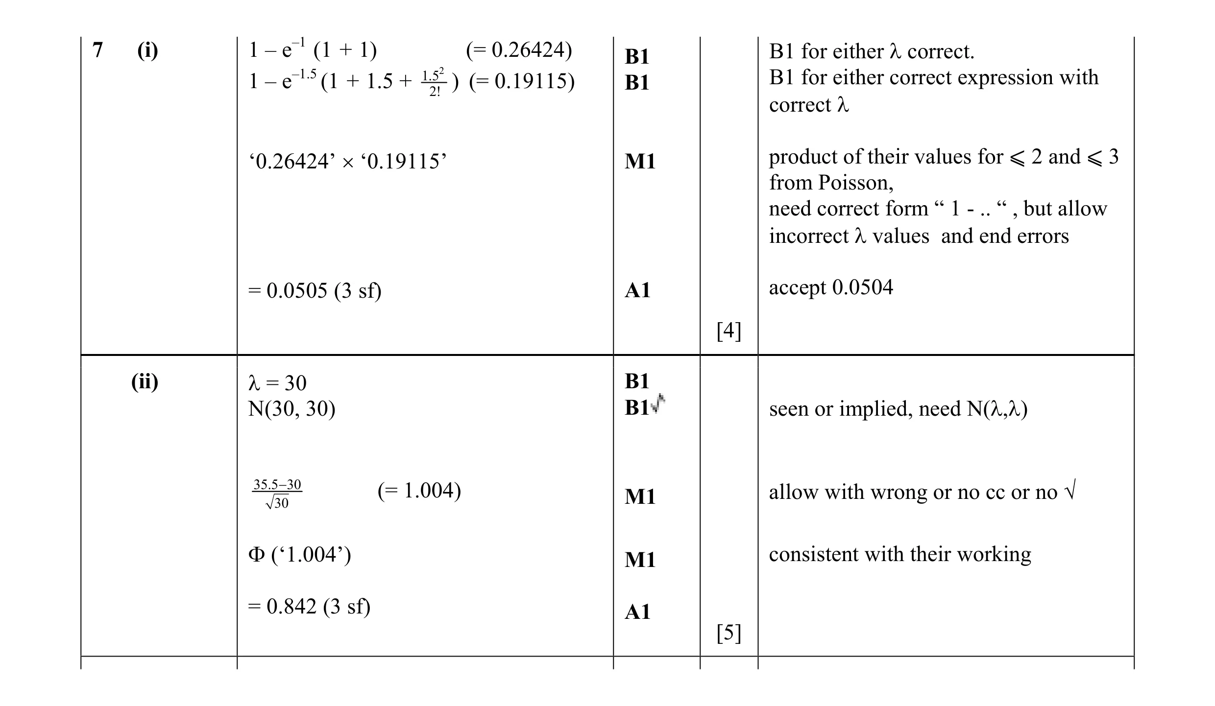 9
9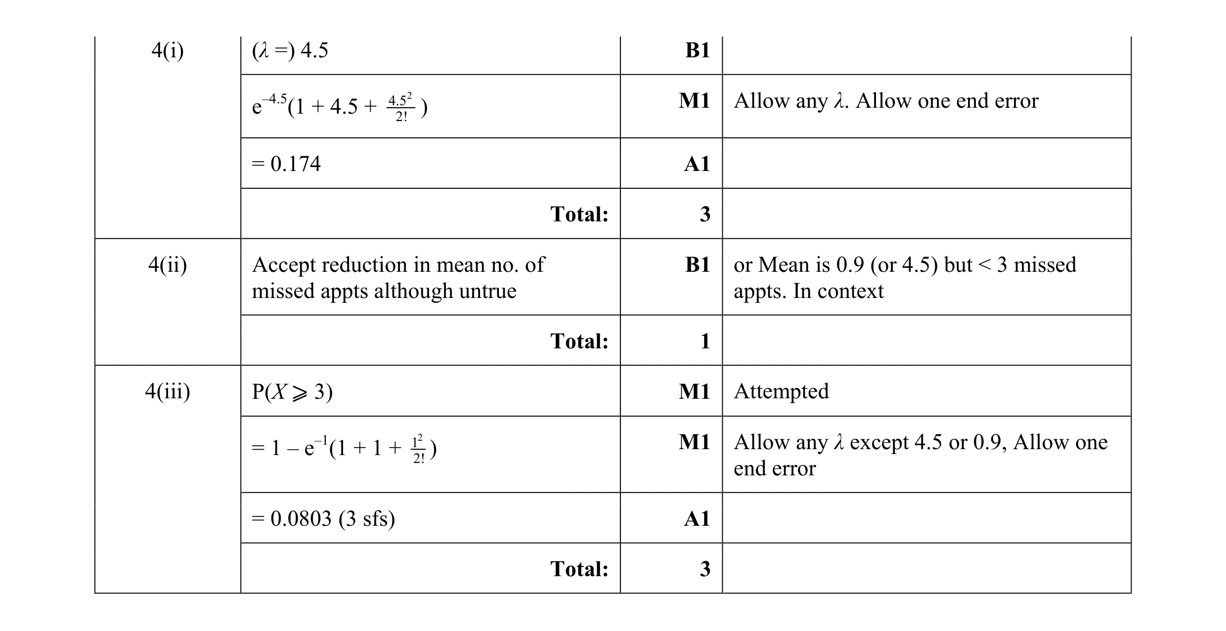 7
7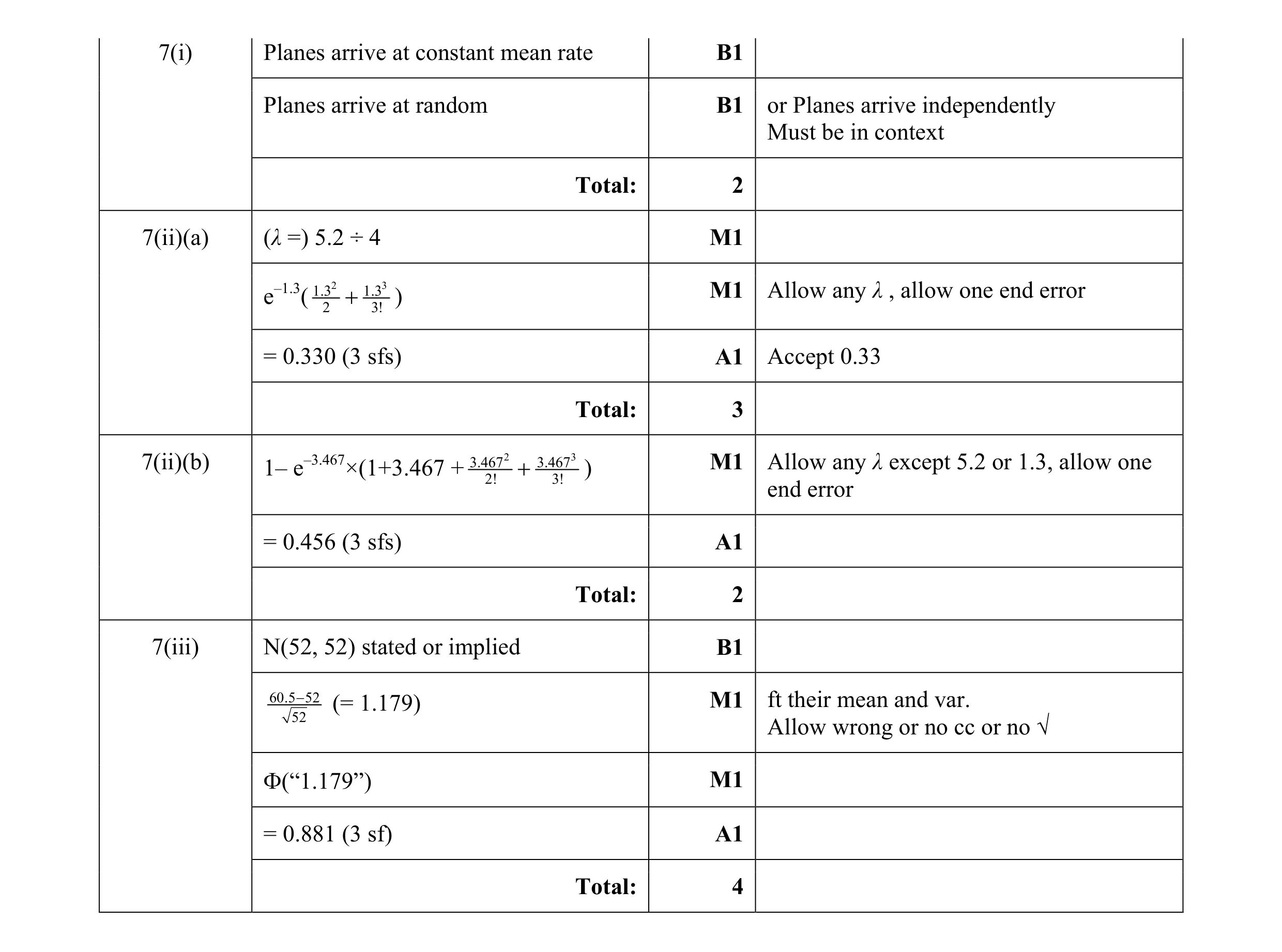 11
11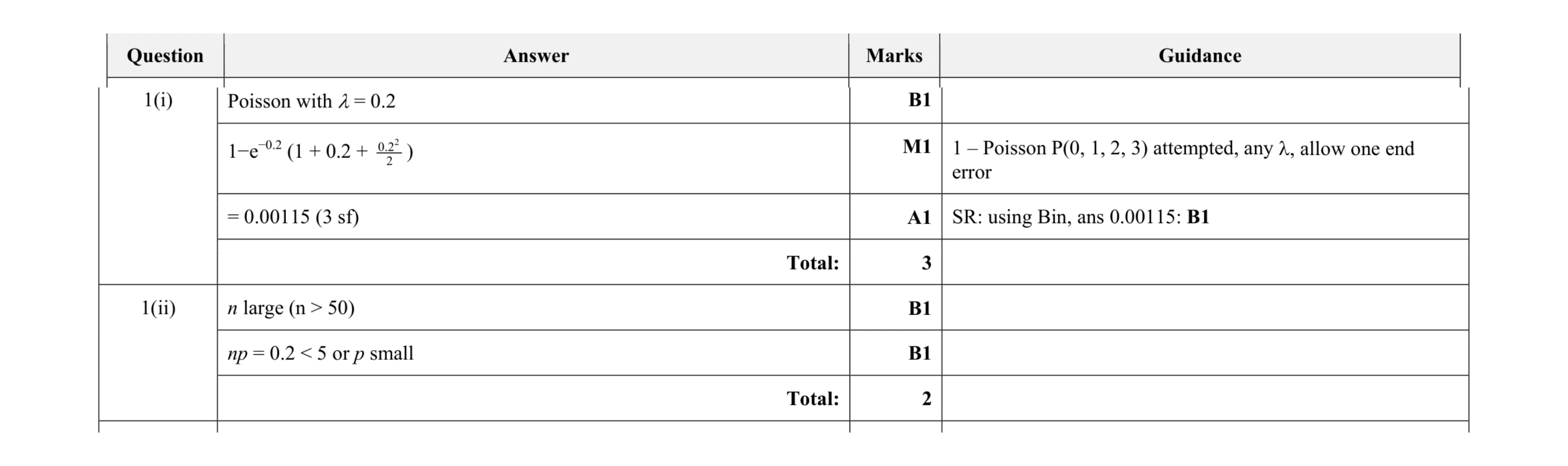 5
5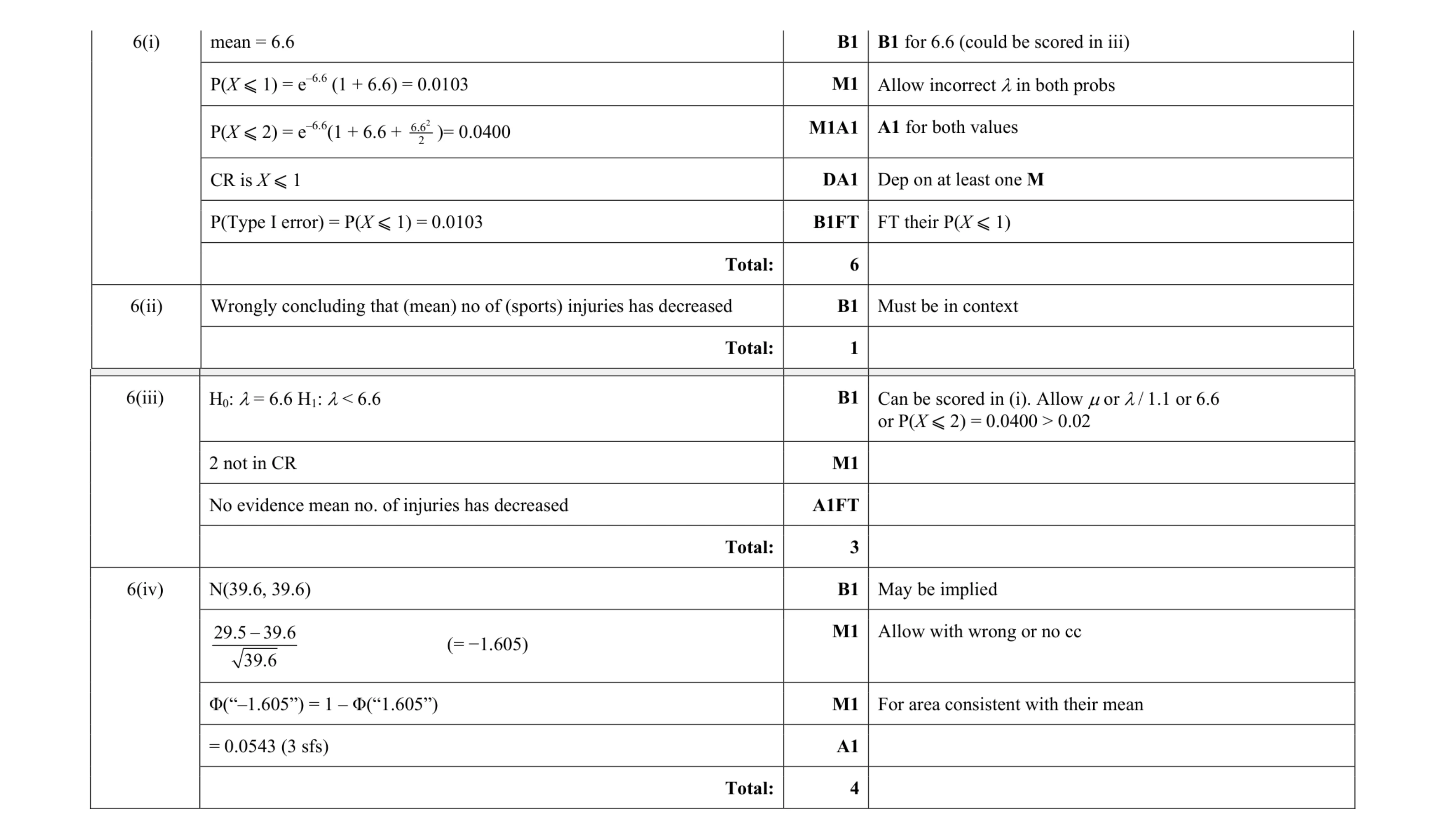 14
14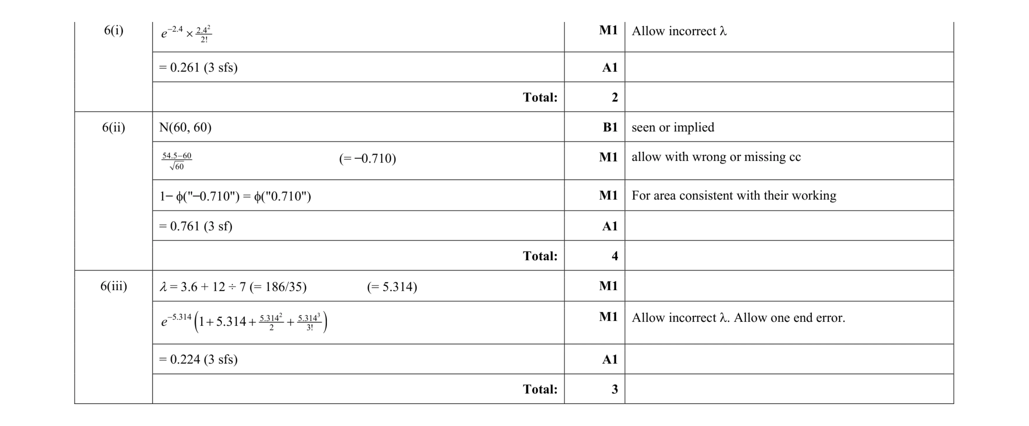 9
9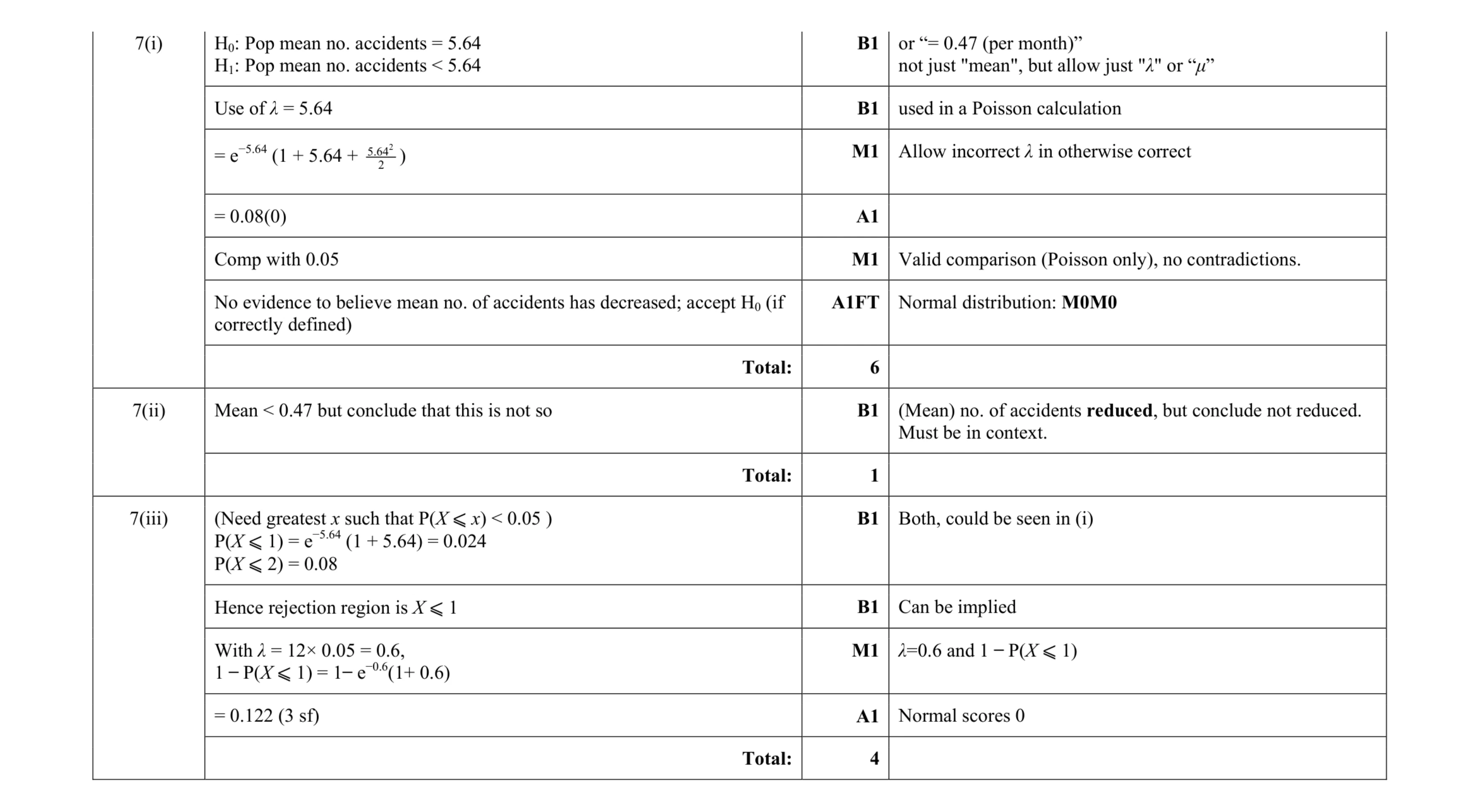 11
11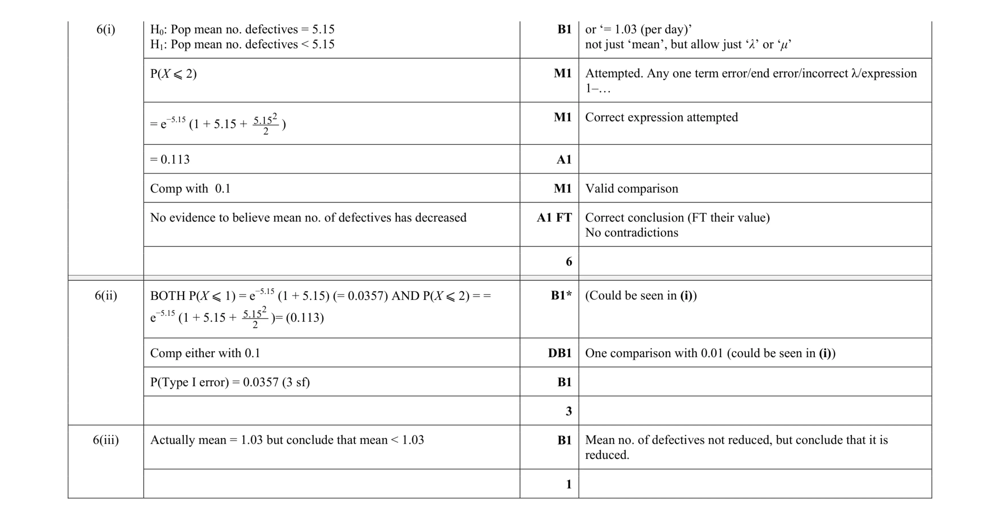 10
10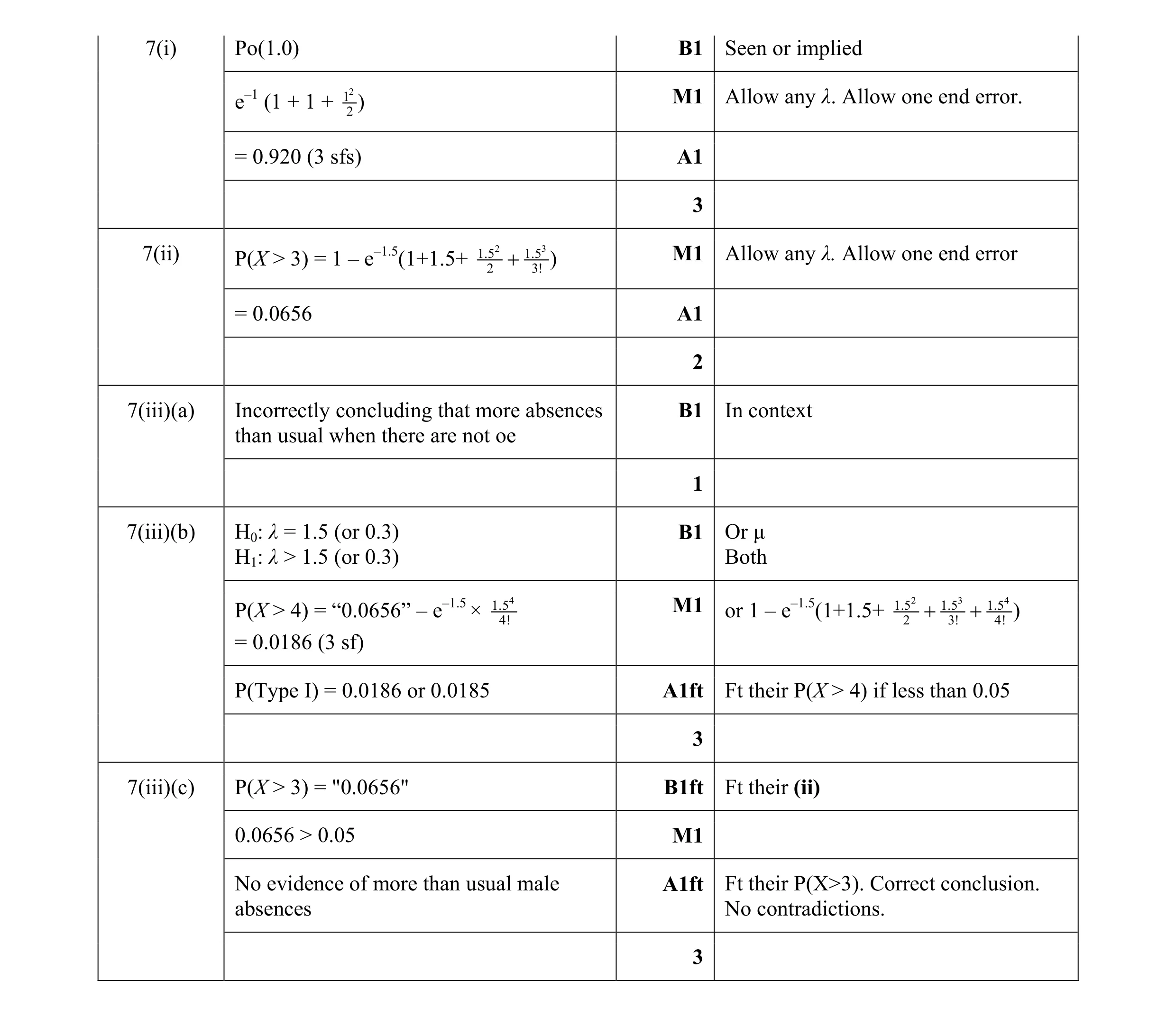 12
12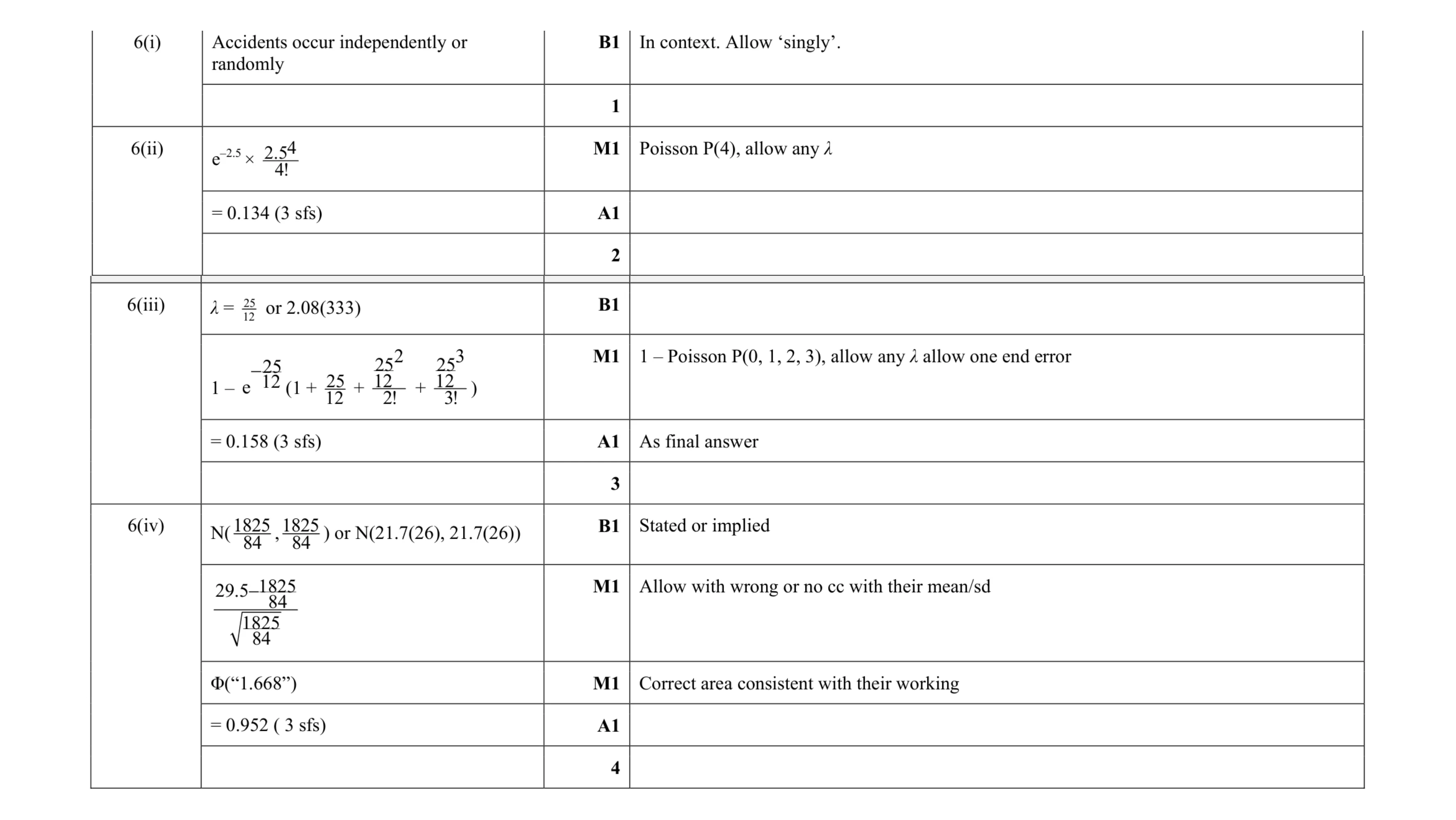 10
10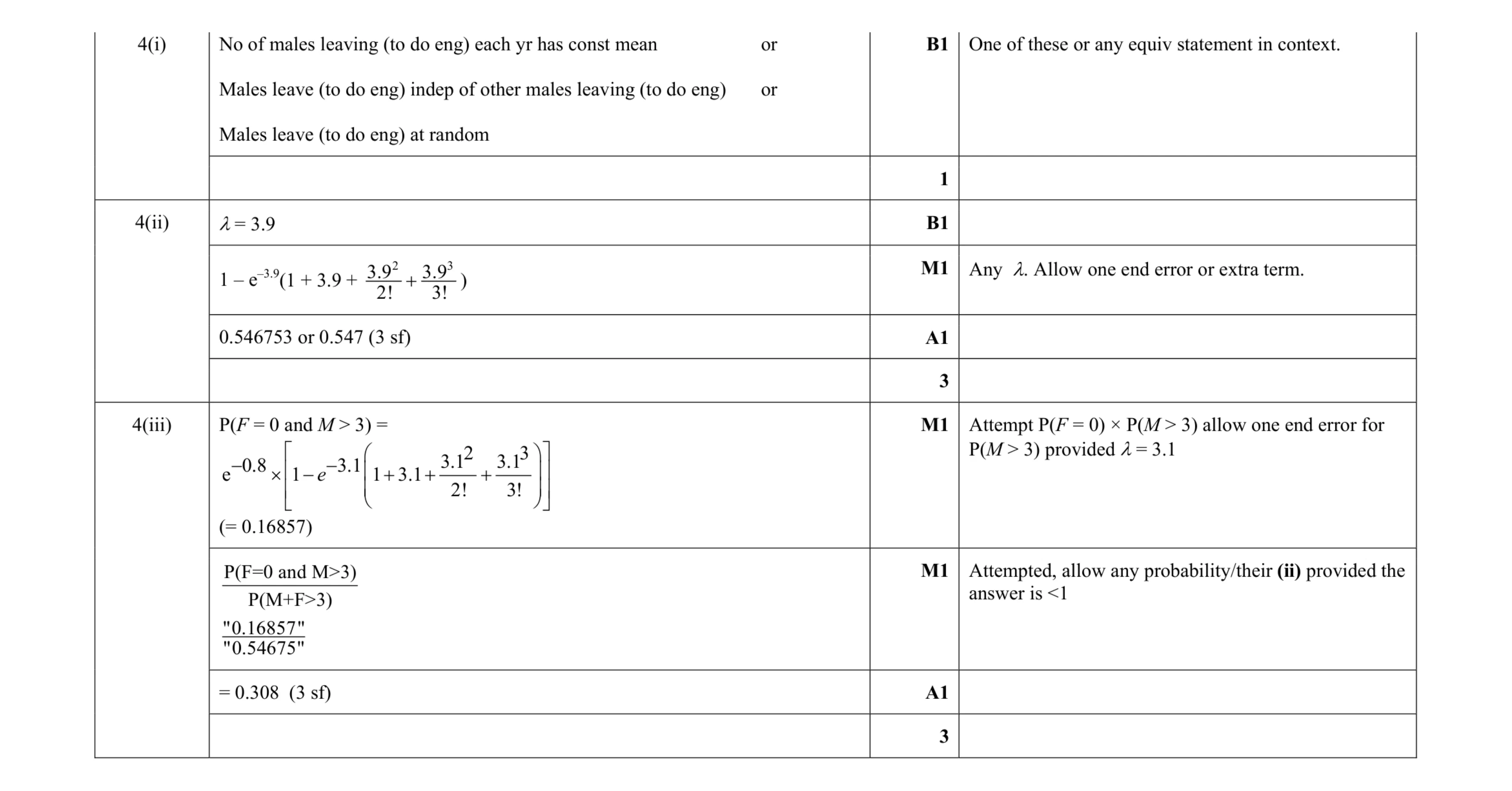 7
7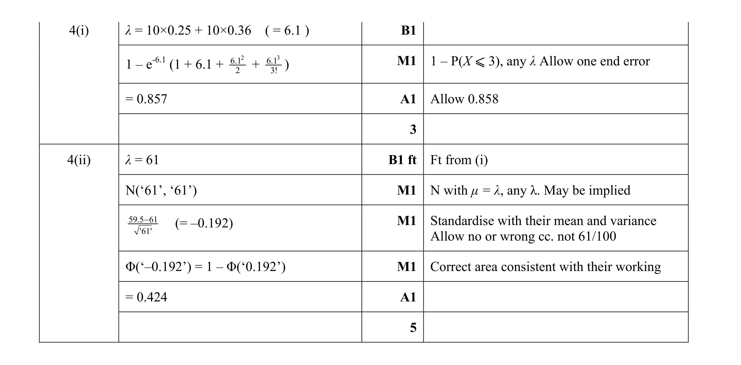 8
8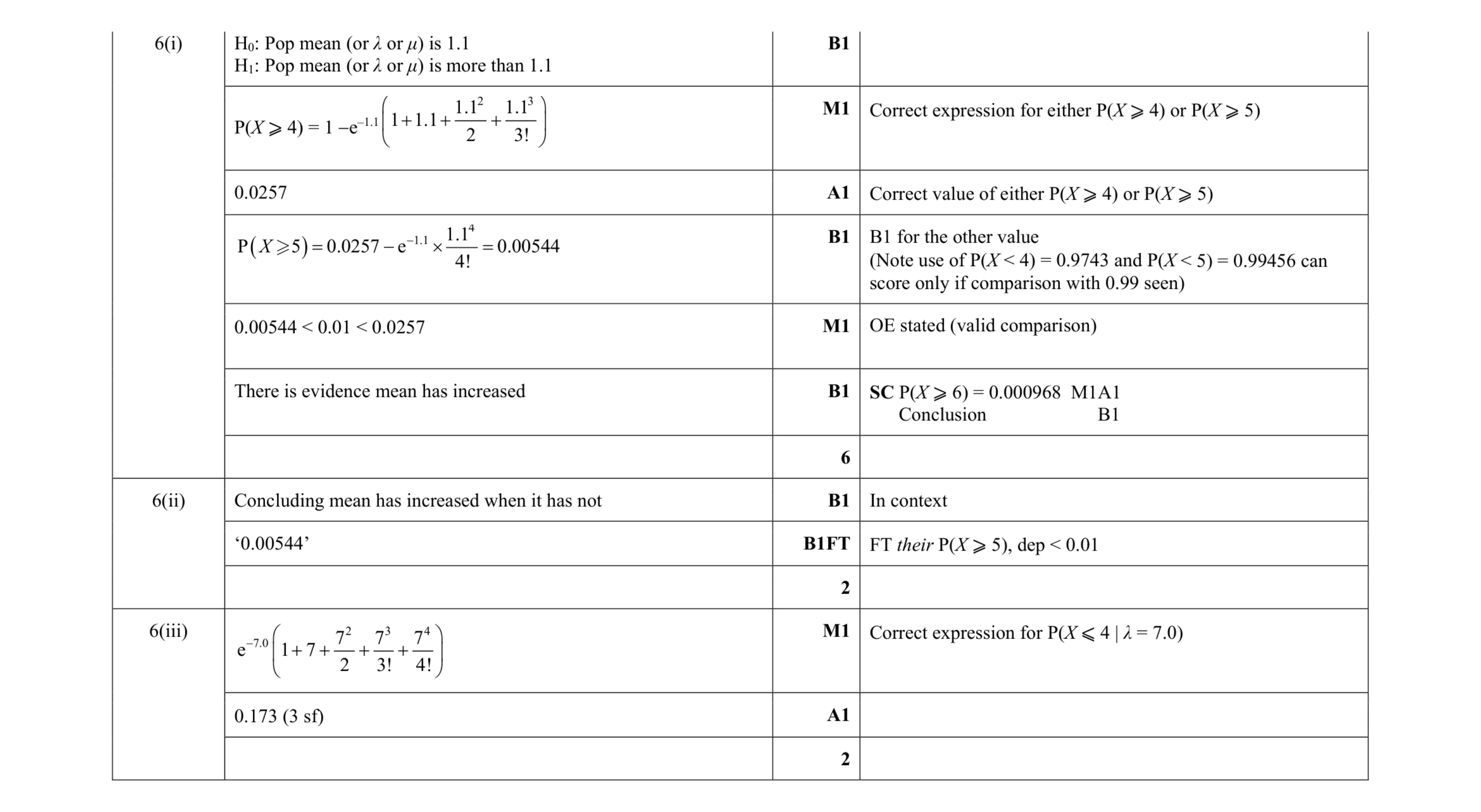 10
10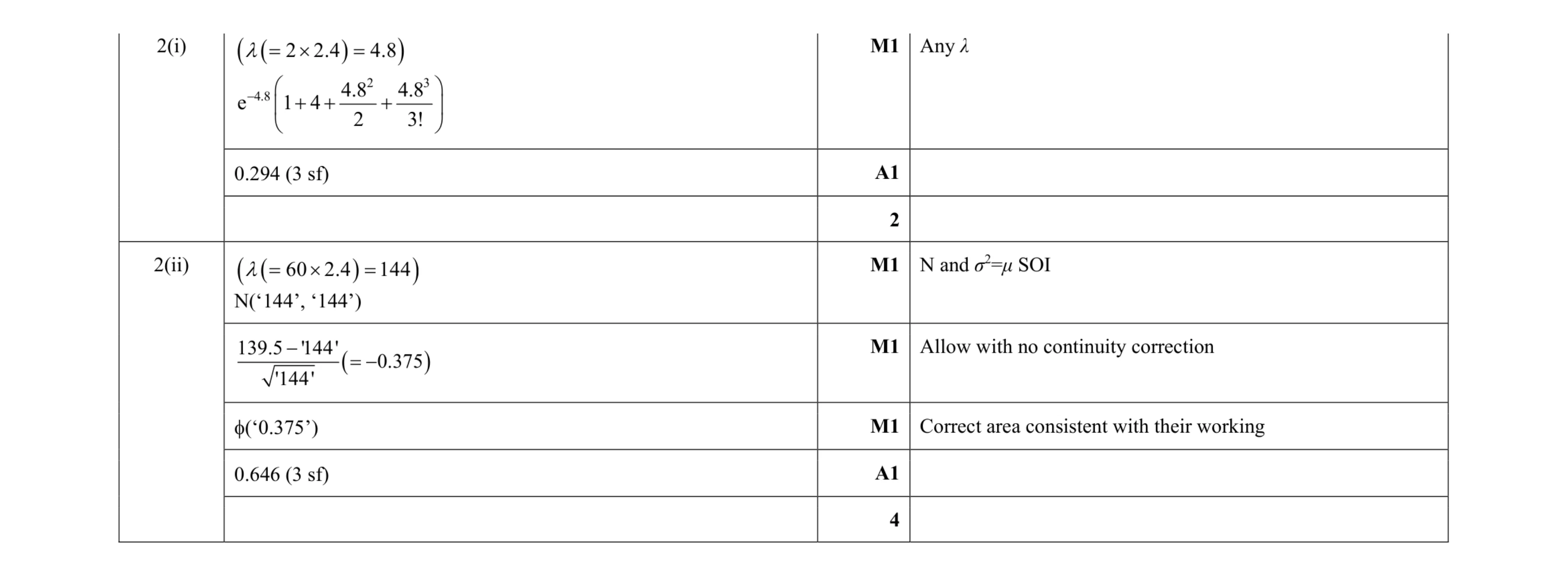 6
6