Questions as text
Q1 · Haroon has 200 letters to post 0580/43 May/June 2017
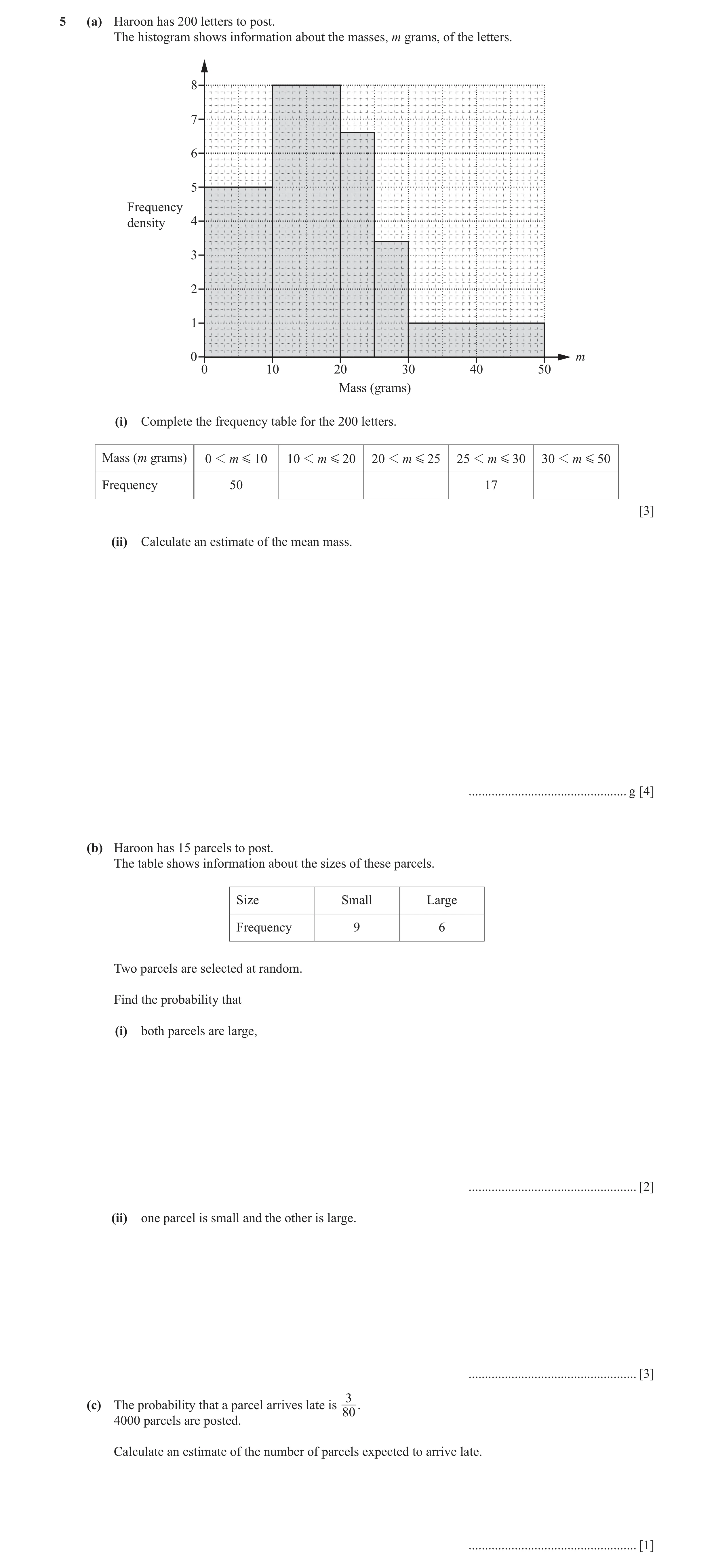
5 (a) Haroon has 200 letters to post. The histogram shows information about the masses, m grams, of the letters. 8 7 6 5 Frequency density 4 3 2 1 0 m 0 10 20 30 40 50 Mass (grams) (i) Complete the frequency table for the 200 letters. Mass (m grams) 0 1 m G 10 10 1 m G 20 20 1 m G 25 25 1 m G 30 30 1 m G 50 Frequency 50 17 [3] (ii) Calculate an estimate of the mean mass. … g [4] (b) Haroon has 15 parcels to post. The table shows information about the sizes of these parcels. Size Small Large Frequency 9 6 Two parcels are selected at random. Find the probability that (i) both parcels are large, … [2] (ii) one parcel is small and the other is large. … [3] 3(c) The probability that a parcel arrives late is . 80 4000 parcels are posted. Calculate an estimate of the number of parcels expected to arrive late. … [1]
13 marks
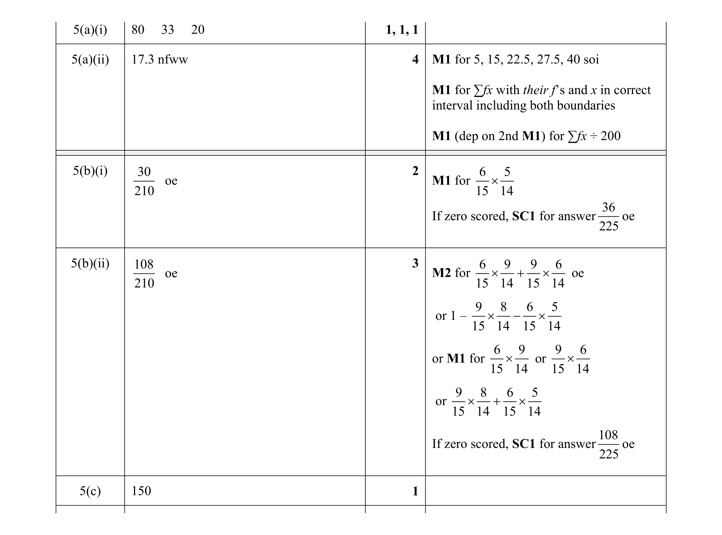
Mark scheme: 5(a)(i) 80 33 20 1, 1, 1 5(a)(ii) 17.3 nfww 4 M1 for 5, 15, 22.5, 27.5, 40 soi M1 for ∑fx with their f’s and x in correct interval including both boundaries M1 (dep on 2nd M1) for ∑fx ÷ 200 5(b)(i) 30 2 6 5 oe M1 for × 210 15 14 36 If zero scored, SC1 for answer oe 225 5(b)(ii) 108 3 6 9 9 6 oe M2 for × + × oe 210 15 14 15 14 9 8 6 5 or 1 – × − × 15 14 15 14 6 9 9 6 or M1 for × or × 15 14 15 14 9 8 6 5 or × + × 15 14 15 14 108 If zero scored, SC1 for answer oe 225 5(c) 150 1
This question in 0580/43 May/June 2017
Q2 · The histogram shows the distribution of the masses, m grams, of 360 apples 0580/41 Oct/Nov 2017
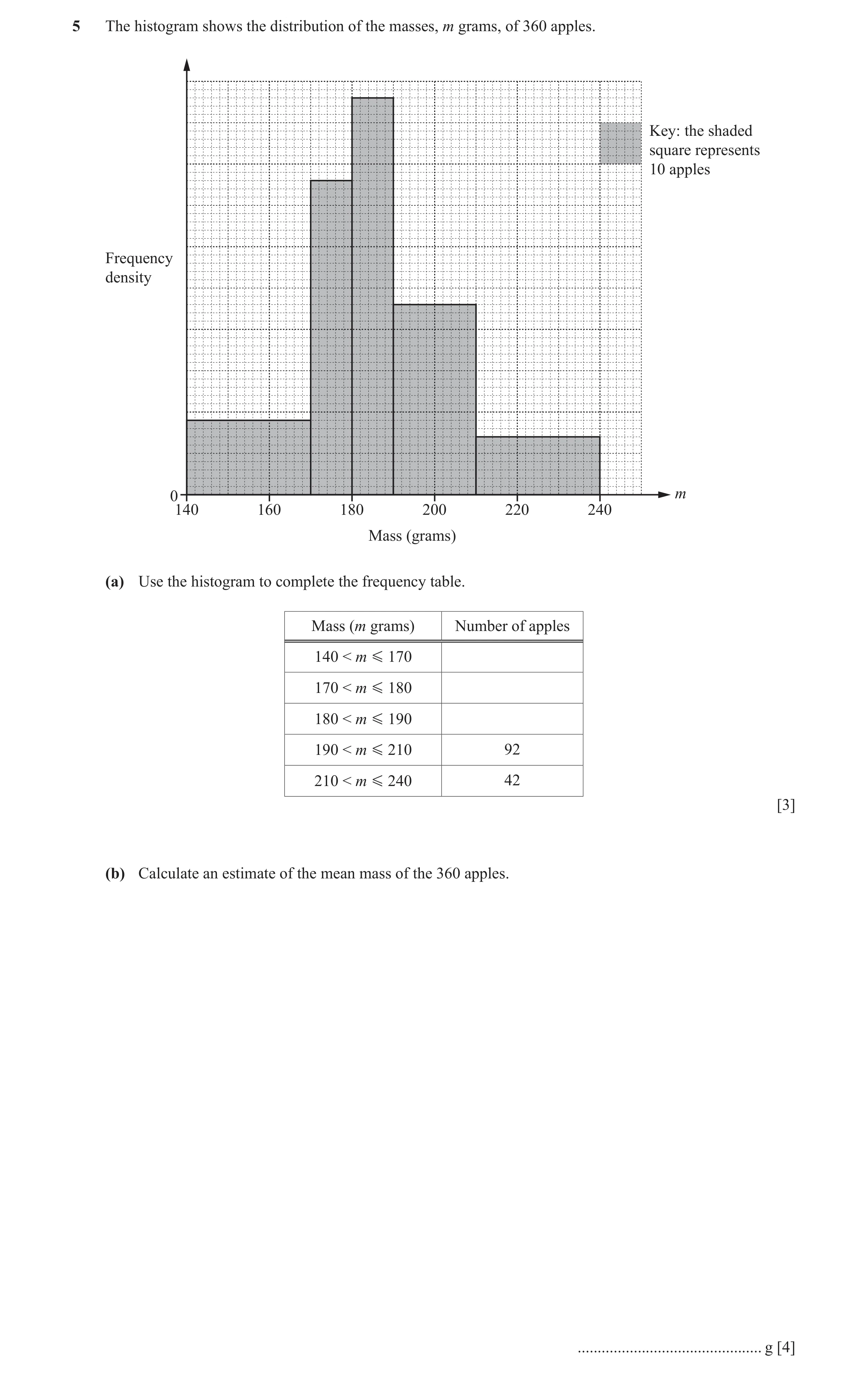
5 The histogram shows the distribution of the masses, m grams, of 360 apples. Key: the shaded square represents 10 apples Frequency density 0 m 140 160 180 200 220 240 Mass (grams) (a) Use the histogram to complete the frequency table. Mass (m grams) Number of apples 140 < m G 170 170 < m G 180 180 < m G 190 190 < m G 210 92 210 < m G 240 42 [3] (b) Calculate an estimate of the mean mass of the 360 apples. … g [4]
7 marks
Mark scheme: 5(a) 54, 76, 96 3 B1 for each 5(b) 187 or 186.8 to 186.9 nfww 4 M1 for 155, 175, 185, 200, 225 soi M1 for Σfm with their frequencies from (a) 155 × their 54 + 175 × their 76 + 185 × their 96 + 200 × 92 + 225 × 42 M1 (dep on second M1) for their Σfm ÷ 360
This question in 0580/41 Oct/Nov 2017
Q3 · The table shows information about the time, t minutes, taken for each of 150 girls to… 0580/43 Oct/Nov 2017
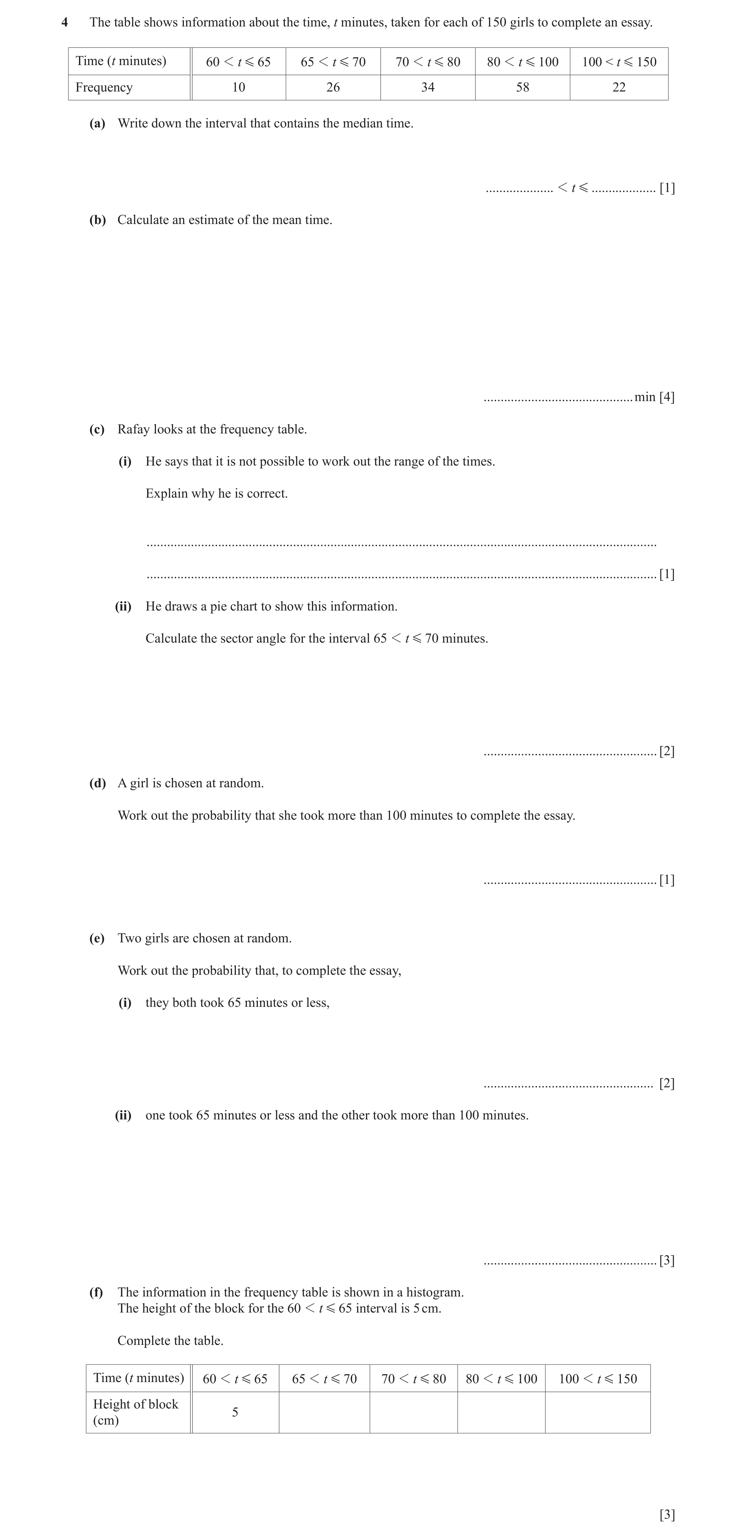
4 The table shows information about the time, t minutes, taken for each of 150 girls to complete an essay. Time (t minutes) 60 1 t G 65 65 1 t G 70 70 1 t G 80 80 1 t G 100 100 < t G 150 Frequency 10 26 34 58 22 (a) Write down the interval that contains the median time. … 1 t G … [1] (b) Calculate an estimate of the mean time. … min [4] (c) Rafay looks at the frequency table. (i) He says that it is not possible to work out the range of the times. Explain why he is correct. … … [1] (ii) He draws a pie chart to show this information. Calculate the sector angle for the interval 65 1 t G 70 minutes. … [2] (d) A girl is chosen at random. Work out the probability that she took more than 100 minutes to complete the essay. … [1] (e) Two girls are chosen at random. Work out the probability that, to complete the essay, (i) they both took 65 minutes or less, … [2] (ii) one took 65 minutes or less and the other took more than 100 minutes. … [3] (f) The information in the frequency table is shown in a histogram. The height of the block for the 60 1 t G 65 interval is 5 cm. Complete the table. Time (t minutes) 60 1 t G 65 65 1 t G 70 70 1 t G 80 80 1 t G 100 100 1 t G 150 Height of block 5 (cm) [3]
17 marks
Mark scheme: 4(a) 80 < t ⩽100 1 4(b) 86 nfww 4 M1 for midpoints soi M1 for use of Σfx with x in correct interval including both boundaries M1 (dep on 2nd M1) for Σfx ÷ 150 4(c)(i) Reference to not knowing the 1 individual values so we do not know the highest or the lowest values 4(c)(ii) 62.4 2 M1 for 26 ÷ 150 or 360 ÷ 150 soi 4(d) 22 1 oe 150 4(e)(i) 90 2 10 9 oe M1 for × 22350 150 149 100 After zero scored, SC1 for answer oe 22500 4(e)(ii) 440 3 10 22 22 10 oe M2 for × + × oe 22350 150 149 150 149 or 10 22 22 10 M1 for × or × oe 150 149 150 149 440 After zero scored, SC1 for answer oe 22500 4(f) 13, 8.5, 7.25, 1.1 3 B2 for 3 correct or B1 for 1 correct or for 3 correct FD.s 5.2, 3.4, 2.9, 0.44 oe
This question in 0580/43 Oct/Nov 2017
Q4 · The scatter diagram shows the physics mark and the chemistry mark for each of 12 students 0580/43 May/June 2018
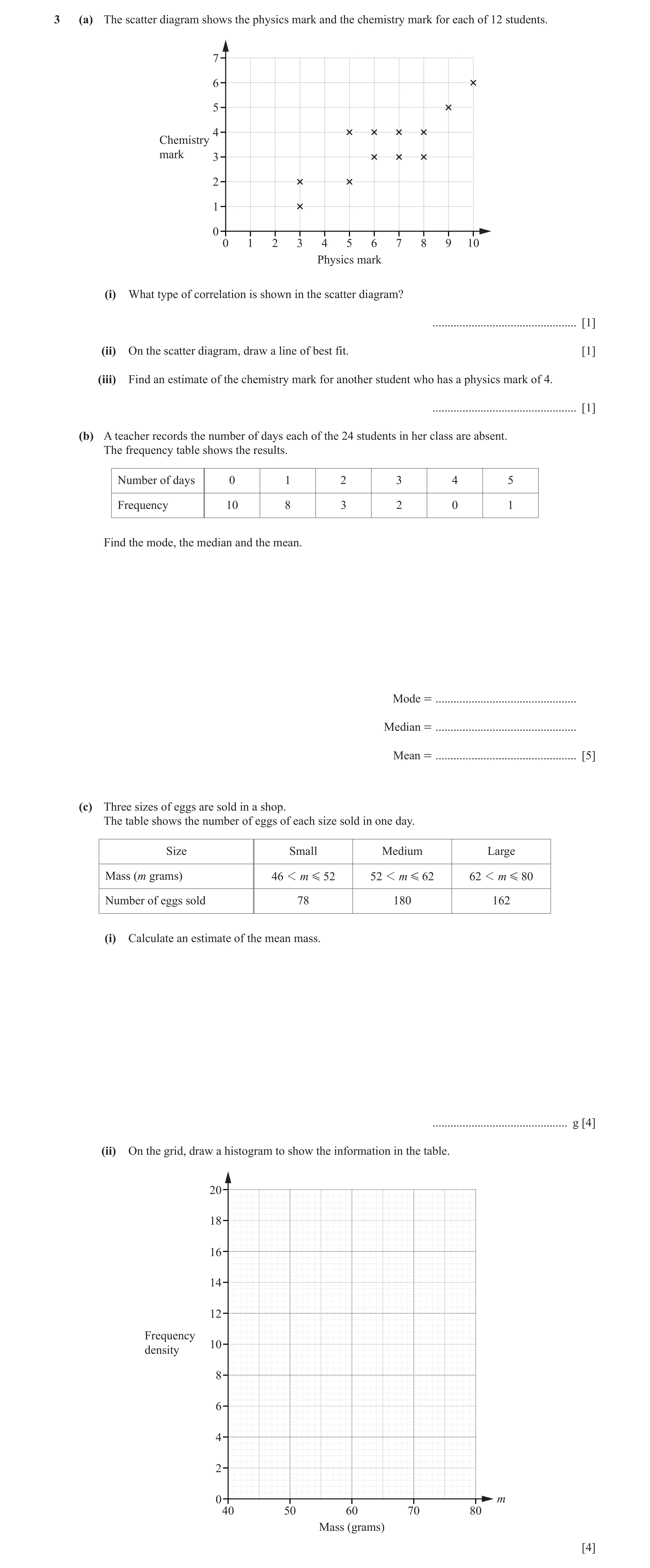
3 (a) The scatter diagram shows the physics mark and the chemistry mark for each of 12 students. 7 6 5 4 Chemistry mark 3 2 1 0 0 1 2 3 4 5 6 7 8 9 10 Physics mark (i) What type of correlation is shown in the scatter diagram? … [1] (ii) On the scatter diagram, draw a line of best fit. [1] (iii) Find an estimate of the chemistry mark for another student who has a physics mark of 4. … [1] (b) A teacher records the number of days each of the 24 students in her class are absent. The frequency table shows the results. Number of days 0 1 2 3 4 5 Frequency 10 8 3 2 0 1 Find the mode, the median and the mean. Mode = … Median = … Mean = … [5] (c) Three sizes of eggs are sold in a shop. The table shows the number of eggs of each size sold in one day. Size Small Medium Large Mass (m grams) 46 1 m G 52 52 1 m G 62 62 1 m G 80 Number of eggs sold 78 180 162 (i) Calculate an estimate of the mean mass. … g [4] (ii) On the grid, draw a histogram to show the information in the table. 20 18 16 14 12 Frequency 10 density 8 6 4 2 0 m 40 50 60 70 80 Mass (grams) [4]
16 marks
Mark scheme: 3(a)(i) Positive 1 Ignore strong, weak, etc. 3(a)(ii) Correct ruled line 1 3(a)(iii) 2 1 3(b) [mode = ] 0 5 B1 [median = ] 1 B1 [mean = ] 1.04 or 1.041 to 1.042 B3 or M2 for ([10 × 0] + 8 × 1 + 3 × 2 + 2 × 3 + [0 × 4] + 1 × 5) ÷ 24 oe or M1 for [10 × 0] + 8 × 1 + 3 × 2 + 2 × 3 + [0 × 4] + 1 × 5 oe 3(c)(i) 60.9 or 60.91... nfww 4 M1 for 49, 57, 71 correct M1 for use of Σfx with x in the correct interval including both boundaries M1 (dep on 2nd M1) for their (78 × 49 + 180 × 57 + 162 × 71) ÷ (78 + 180 + 162) 3(c)(ii) Correct histogram 4 B1 for correct widths in correct position B1 height 13 B1 height 18 B1 height 9 If 0 scored B1 for 13, 18 and 9 seen
This question in 0580/43 May/June 2018
Q5 · A school nurse records the height, h cm, of each of 180 children 0580/41 Oct/Nov 2018
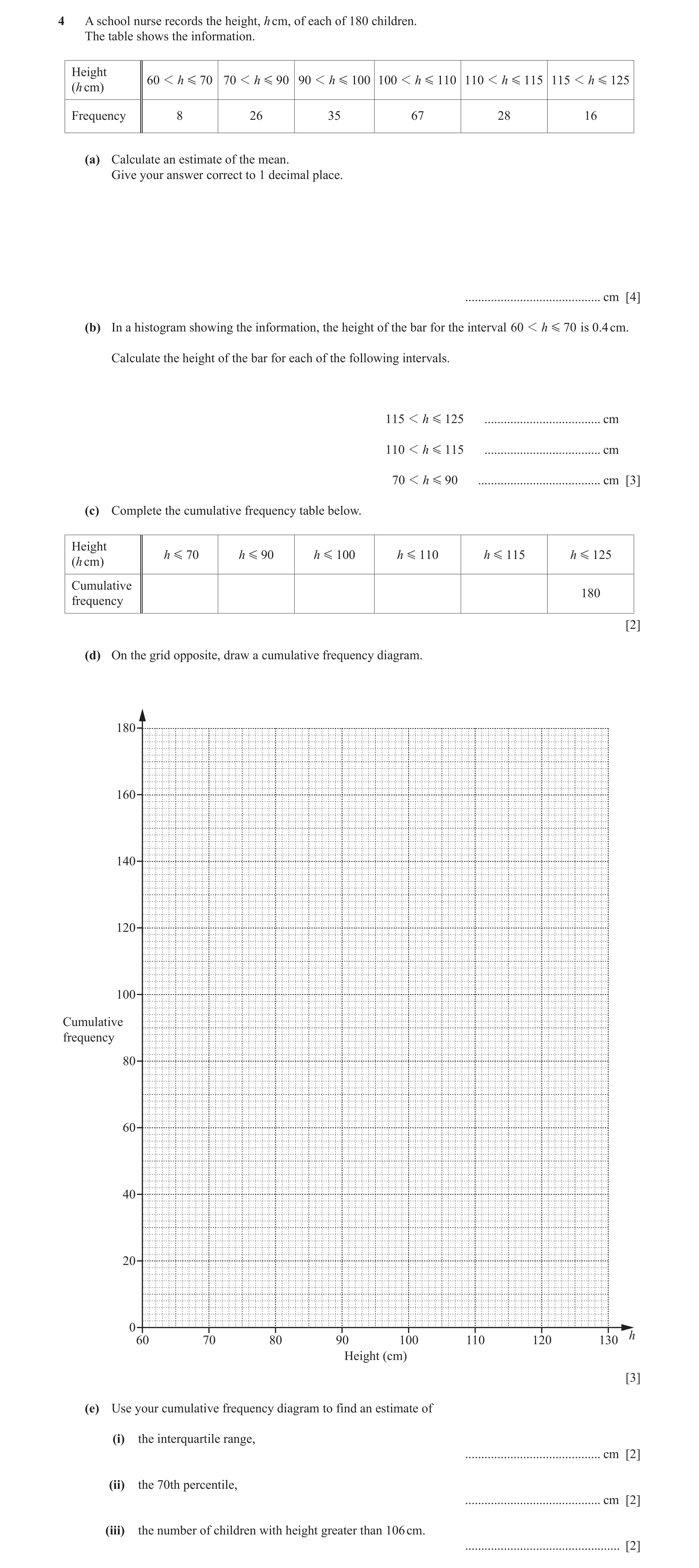
4 A school nurse records the height, h cm, of each of 180 children. The table shows the information. Height 60 1 h G 70 70 1 h G 90 90 1 h G 100 100 1 h G 110 110 1 h G 115 115 1 h G 125 (h cm) Frequency 8 26 35 67 28 16 (a) Calculate an estimate of the mean. Give your answer correct to 1 decimal place. … cm [4] (b) In a histogram showing the information, the height of the bar for the interval 60 1 h G 70 is 0.4 cm. Calculate the height of the bar for each of the following intervals. 115 1 h G 125 … cm 110 1 h G 115 … cm 70 1 h G 90 … cm [3] (c) Complete the cumulative frequency table below. Height h G 70 h G 90 h G 100 h G 110 h G 115 h G 125 (h cm) Cumulative 180 frequency [2] (d) On the grid opposite, draw a cumulative frequency diagram.
18 marks
Mark scheme: 4(a) 100.2 nfww 4 M1 for midpoints soi 65, 80, 95, 105, 112.5, 120 M1 for use of ∑fx with x in correct interval including both boundaries M1dep for ∑fx ÷ 180 dep on previous M1 4(b) 0.8 3 B1 for each 2.8 If zero scored, SC1 for 1.6, 5.6 and 1.3 0.65 seen 4(c) 8 34 69 136 164 2 B1 for one error FT other values or for 3 or 4 correct 4(d) Correct diagram 3 B1FT for correct vertical placement for 6 plots B1 for correct horizontal placement for 6 plots B1FT dep on at least B1 for reasonable increasing curve or polygon through their 6 points If zero scored, SC1FT for 5 out of 6 correct plots 4(e)(i) 15 to 17 2 B1 for [LQ =] 93 to 94 or [UQ =] 109 to 110 4(e)(ii) 107 to 109 2 B1 for 126 seen 4(e)(iii) 66 to 72 2 FT their graph for 2 marks B1 for answer 106 to 114 or B1FT their graph reading at 106 cm seen
This question in 0580/41 Oct/Nov 2018
Q6 · A factory recycles metal 0580/43 Oct/Nov 2018
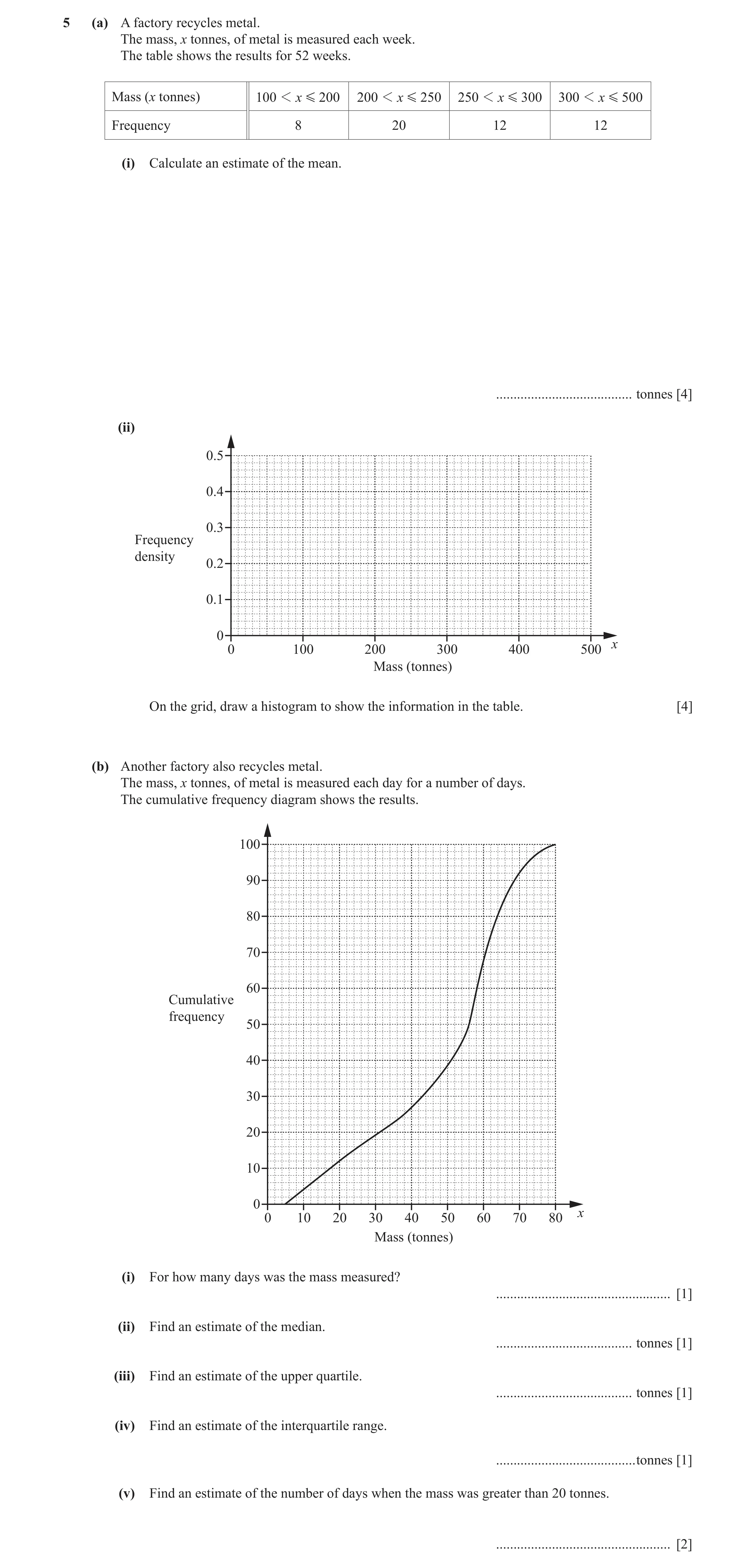
5 (a) A factory recycles metal. The mass, x tonnes, of metal is measured each week. The table shows the results for 52 weeks. Mass (x tonnes) 100 1 x G 200 200 1 x G 250 250 1 x G 300 300 1 x G 500 Frequency 8 20 12 12 (i) Calculate an estimate of the mean. … tonnes [4] (ii) 0.5 0.4 0.3 Frequency density 0.2 0.1 0 x 0 100 200 300 400 500 Mass (tonnes) On the grid, draw a histogram to show the information in the table. [4] (b) Another factory also recycles metal. The mass, x tonnes, of metal is measured each day for a number of days. The cumulative frequency diagram shows the results. 100 90 80 70 60 Cumulative frequency 50 40 30 20 10 0 x 0 10 20 30 40 50 60 70 80 Mass (tonnes) (i) For how many days was the mass measured? … [1] (ii) Find an estimate of the median. … tonnes [1] (iii) Find an estimate of the upper quartile. … tonnes [1] (iv) Find an estimate of the interquartile range. … tonnes [1] (v) Find an estimate of the number of days when the mass was greater than 20 tonnes. … [2]
14 marks
Mark scheme: 5(a)(i) 265 or 265.3 to 265.4 nfww 4 M1 for mid-values 150, 225, 275, 400 soi M1 for Σ fx where x is in correct interval including boundaries M1 dep for Σ fx ÷ 52 dependent on second M1 5(a)(ii) Correct histogram 4 B1 for each correct block If 0 scored, SC1 for the four frequency densities seen 5(b)(i) 100 1 5(b)(ii) 56 1 5(b)(iii) 62 1 5(b)(iv) 24 1 5(b)(v) 88 2 M1 for evidence of 12 written
This question in 0580/43 Oct/Nov 2018
Q7 · The table shows the time, t seconds, taken by each of 120 boys to solve a puzzle 0580/43 May/June 2019
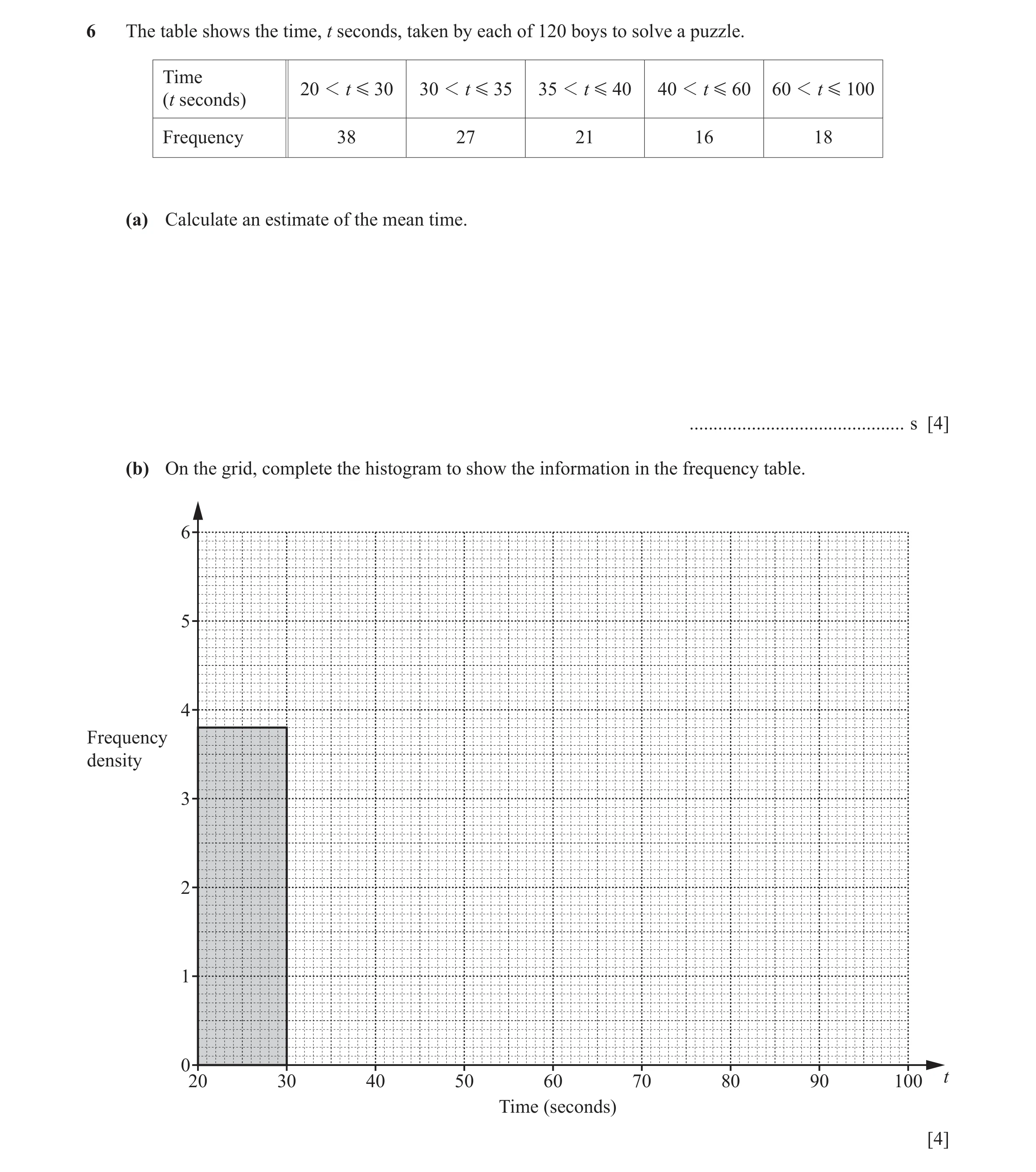
6 The table shows the time, t seconds, taken by each of 120 boys to solve a puzzle. Time 20 1 t G 30 30 1 t G 35 35 1 t G 40 40 1 t G 60 60 1 t G 100 (t seconds) Frequency 38 27 21 16 18 (a) Calculate an estimate of the mean time. … s [4] (b) On the grid, complete the histogram to show the information in the frequency table. 6 5 4 Frequency density 3 2 1 0 20 30 40 50 60 70 80 90 100 t Time (seconds) [4]
8 marks
Mark scheme: 6(a) 40.5 or 40.45[8..] or 40.46 nfww 4 M1 for 25, 32.5, 37.5, 50, 80 soi M1 for Σft M1 dep for theirΣft ÷ 120 6(b) Fully correct histogram 4 B1 for each correct bar If 0 scored, SC1 for frequency densities of 5.4, 4.2, 0.8 and 0.45 seen
This question in 0580/43 May/June 2019
Q8 · The cumulative frequency diagram shows information about the times taken by 200 students… 0580/41 Oct/Nov 2019
6 (a) The cumulative frequency diagram shows information about the times taken by 200 students to solve a problem. 200 180 160 140 120 Cumulative 100 frequency 80 60 40 20 0 0 10 20 30 40 50 60 Time (minutes) Use the cumulative frequency diagram to find an estimate for (i) the median, … min [1] (ii) the interquartile range, … min [2] (iii) the number of students who took more than 40 minutes. … [2] (b) Roberto records the value of each of the coins he has at home. The table shows the results. Value (cents) 1 2 5 10 20 50 Frequency 3 1 3 2 4 2 (i) Find the range. … cents [1] (ii) Find the mode. … cents [1] (iii) Find the median. … cents [1] (iv) Work out the total value of Roberto’s coins. … cents [2] (v) Work out the mean. … cents [1] (c) The histogram shows information about the masses of 100 boxes. 10 9 8 7 6 Frequency 5 density 4 3 2 1 0 0 5 10 15 20 25 30 Mass (kilograms) Calculate an estimate of the mean. … kg [6]
17 marks
Mark scheme: 6(a)(i) 34 1 6(a)(ii) 18 2 B1 for [l.q. = ] 25 or [u.q. = ] 43 seen 6(a)(iii) 60 2 M1 for 140 written 6(b)(i) 49 1 6(b)(ii) 20 1 6(b)(iii) 10 1 6(b)(iv) 220 2 M1 for 3 × 1 + 1 × 2 + 3 × 5 + 2 × 10 + 4 × 20 + 2 × 50 6(b)(v) 14.7 or 14.66 to 14.67 1 FT their (iv) ÷ 15 6(c) 13.25 nfww 6 B2 for frequencies 30, 40, 30 soi or B1 for 2 of these M1 for 5, 12.5, 22.5 M1 Σ fx with their frequencies (if seen) and each x in correct interval including boundaries Σfx M1 dependent for (dependent on 100 second M1) OR Alternative Method B2 for frequencies 15, 15, 40, 10, 10, 10 soi or B1 for 2 of 15, 40, 10 M1 for 2.5, 7.5, 12.5, 17.5, 22.5, 27.5 M1 Σ fx with their frequencies (if seen) and each x in correct interval including boundaries Σfx M1 dependent for (dependent on 100 second M1)
This question in 0580/41 Oct/Nov 2019
Q9 · The speed, v km/h, of each of 200 cars passing a building is measured 0580/42 May/June 2020
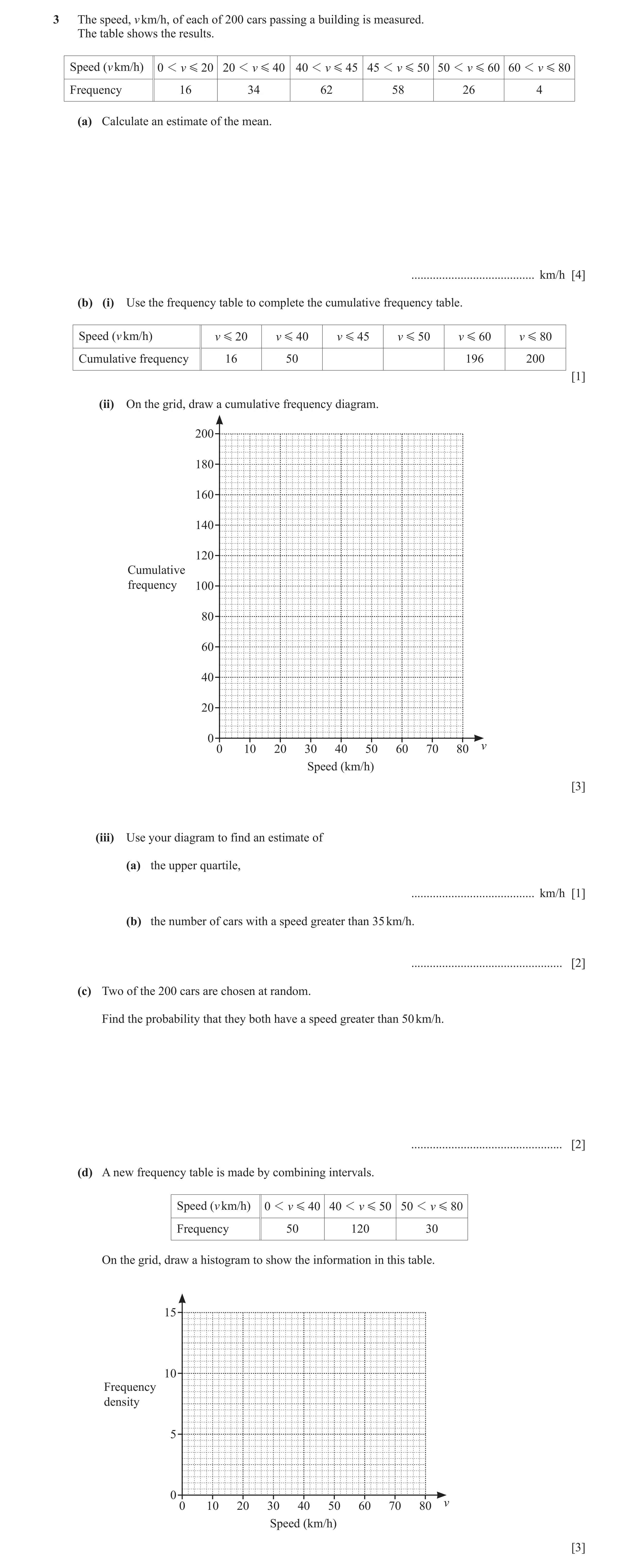
3 The speed, v km/h, of each of 200 cars passing a building is measured. The table shows the results. Speed (v km/h) 0 1 v G 20 20 1 v G 40 40 1 v G 45 45 1 v G 50 50 1 v G 60 60 1 v G 80 Frequency 16 34 62 58 26 4 (a) Calculate an estimate of the mean. … km/h [4] (b) (i) Use the frequency table to complete the cumulative frequency table. Speed (v km/h) v G 20 v G 40 v G 45 v G 50 v G 60 v G 80 Cumulative frequency 16 50 196 200 [1] (ii) On the grid, draw a cumulative frequency diagram. 200 180 160 140 120 Cumulative frequency 100 80 60 40 20 0 v 0 10 20 30 40 50 60 70 80 Speed (km/h) [3] (iii) Use your diagram to find an estimate of (a) the upper quartile, … km/h [1] (b) the number of cars with a speed greater than 35 km/h. … [2] (c) Two of the 200 cars are chosen at random. Find the probability that they both have a speed greater than 50 km/h. … [2] (d) A new frequency table is made by combining intervals. Speed (v km/h) 0 1 v G 40 40 1 v G 50 50 1 v G 80 Frequency 50 120 30 On the grid, draw a histogram to show the information in this table. 15 10 Frequency density 5 0 v 0 10 20 30 40 50 60 70 80 Speed (km/h) [3]
16 marks
Mark scheme: 3(a) 41.4 4 M1 for 10, 30, 42.5, 47.5, 55, 70 M1 for Σ fx where x lies in or on the boundary of each interval. Σfx M1 dep for dep on second M1 200 3(b)(i) 112, 170 1 3(b)(ii) Correct diagram 3 B1 for correct horizontal plot B1FT for correct vertical plots B1 FT dep on at least B1 earned for reasonable increasing curve or polygon through their 6 points If 0 scored SC1FT for 5 out of 6 points plotted correctly 3(b)(iii)(a) 48 1 3(b)(iii)(b) 160 2 M1 for 40 seen 3(c) 87 2 30 29 oe M1 for × oe 3980 200 199 3(d) Correct histogram 3 B1 for each column If 0 scored SC1 for correct frequency densities soi 1.25, 12, 1
This question in 0580/42 May/June 2020
Q10 · The height, h cm, of each of 120 plants is measured 0580/42 Oct/Nov 2020
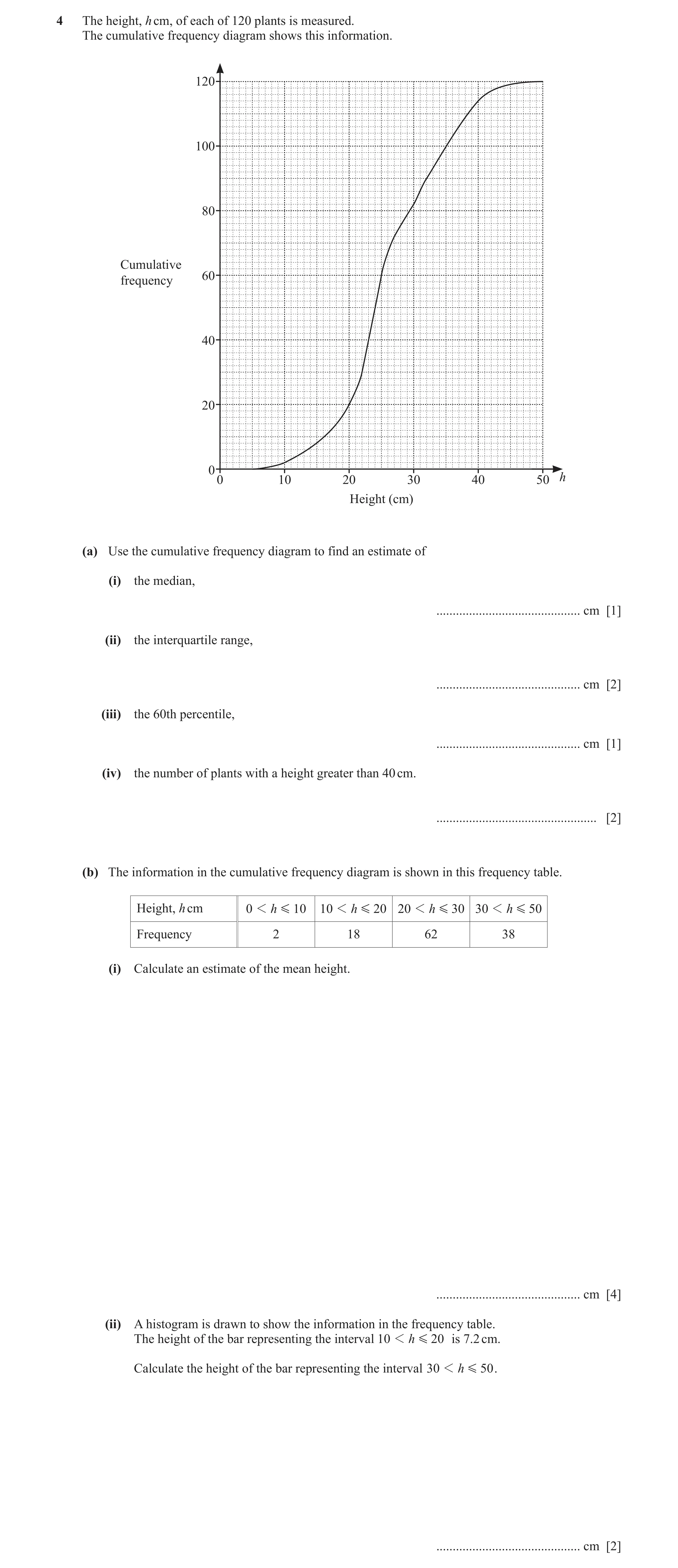
4 The height, h cm, of each of 120 plants is measured. The cumulative frequency diagram shows this information. 120 100 80 Cumulative 60 frequency 40 20 0 0 10 20 30 40 50 h Height (cm) (a) Use the cumulative frequency diagram to find an estimate of (i) the median, … cm [1] (ii) the interquartile range, … cm [2] (iii) the 60th percentile, … cm [1] (iv) the number of plants with a height greater than 40 cm. … [2] (b) The information in the cumulative frequency diagram is shown in this frequency table. Height, h cm 0 1 h G 10 10 1 h G 20 20 1 h G 30 30 1 h G 50 Frequency 2 18 62 38 (i) Calculate an estimate of the mean height. … cm [4] (ii) A histogram is drawn to show the information in the frequency table. The height of the bar representing the interval 10 1 h G 20 is 7.2 cm. Calculate the height of the bar representing the interval 30 1 h G 50 . … cm [2]
12 marks
Mark scheme: 4(a)(i) 25 1 4(a)(ii) 10 nfww 2 B1 for [lq =] 22 or [uq =] 32 4(a)(iii) 27 1 4(a)(iv) 6 2 B1 for 114 written 4(b)(i) 27.9 or 27.91 to 27.92 nfww 4 M1 for mid-values M1 where x lies within or on forfx boundary of correct interval M1 dep ÷ 120 dep on second M1 fx 4(b)(ii) 7.6 2 18 38 M1 for oe or oe 10 20 or B1 for [multiplier] 4 or ¼
This question in 0580/42 Oct/Nov 2020
Q11 · The mass, m kg, of each of 40 parcels in a warehouse is recorded 0580/42 May/June 2021
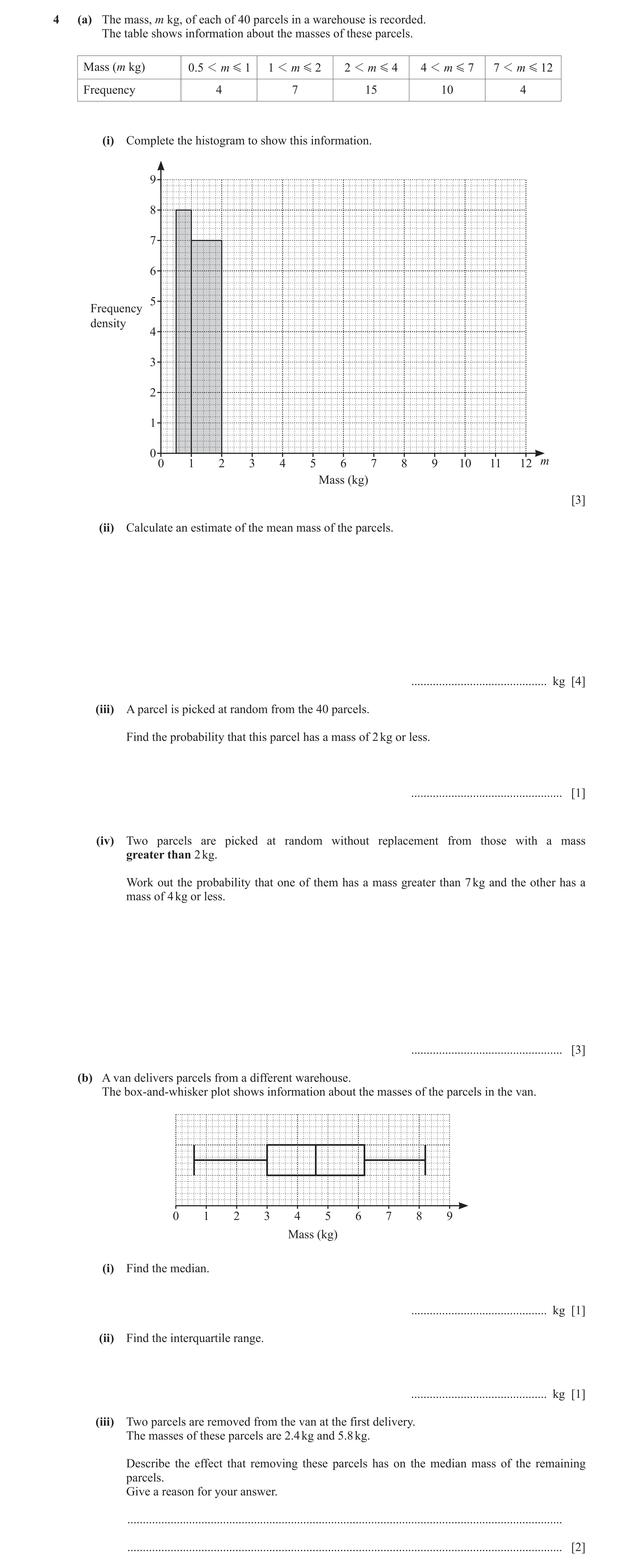
4 (a) The mass, m kg, of each of 40 parcels in a warehouse is recorded. The table shows information about the masses of these parcels. Mass (m kg) 0.5 1 m G 1 1 1 m G 2 2 1 m G 4 4 1 m G 7 7 1 m G 12 Frequency 4 7 15 10 4 (i) Complete the histogram to show this information. 9 8 7 6 5 Frequency density 4 3 2 1 0 0 1 2 3 4 5 6 7 8 9 10 11 12 m Mass (kg) [3] (ii) Calculate an estimate of the mean mass of the parcels. … kg [4] (iii) A parcel is picked at random from the 40 parcels. Find the probability that this parcel has a mass of 2 kg or less. … [1] (iv) Two parcels are picked at random without replacement from those with a mass greater than 2 kg. Work out the probability that one of them has a mass greater than 7 kg and the other has a mass of 4 kg or less. … [3] (b) A van delivers parcels from a different warehouse. The box-and-whisker plot shows information about the masses of the parcels in the van. 0 1 2 3 4 5 6 7 8 9 Mass (kg) (i) Find the median. … kg [1] (ii) Find the interquartile range. … kg [1] (iii) Two parcels are removed from the van at the first delivery. The masses of these parcels are 2.4 kg and 5.8 kg. Describe the effect that removing these parcels has on the median mass of the remaining parcels. Give a reason for your answer. … … [2]
15 marks
Mark scheme: 4(a)(i) Correct histogram 3 B1 for each correct block If 0 scored, SC1 for any two of fds 7.5, 3.33…, 0.8 oe soi 4(a)(ii) 3.7875 or 3.79 or 3.787 or 3.788 4 M1 for 0.75, 1.5, 3, 5.5, 9.5 soi M1 for Σfx M1 dep for their Σfx ÷ 40 4(a)(iii) 11 1 oe 40 4(a)(iv) 30 3 4 15 oe M2 for [2 ×] × oe 203 29 28 4 15 or M1 for or oe seen 29 29 4 26 After 0 scored, SC1 for [ 2 ×] × 40 39 oe 120 or for answer oe 841 4(b)(i) 4.6 1 4(b)(ii) 3.2 1 4(b)(iii) [median] remains the same oe 2 B1 for each statement and one is below [the median/middle] and one is above oe
This question in 0580/42 May/June 2021
Q12 · Zoe’s test scores last term were 6 7 7 7 8 9 9 10 10 0580/43 May/June 2021
3 (a) Zoe’s test scores last term were 6 7 7 7 8 9 9 10 10. Find (i) the range, … [1] (ii) the mode, … [1] (iii) the median. … [1] (b) The cumulative frequency diagram shows information about the time taken by each of 200 students to solve a problem. 200 180 160 140 120 Cumulative 100 frequency 80 60 40 20 0 0 2 4 6 8 10 12 14 16 18 20 Time (minutes) Use the diagram to find an estimate of (i) the median, … min [1] (ii) the interquartile range. … min [2] (c) The test scores of 200 students are shown in the table. Score 5 6 7 8 9 10 Frequency 3 10 43 75 48 21 Calculate the mean. … [3] (d) The height, in cm, of each of 200 plants is measured. The histogram shows the results. 4 3 Frequency 2 density 1 0 50 60 70 80 90 100 110 120 130 140 150 160 Height (cm) Calculate an estimate of the mean height. You must show all your working. … cm [6]
15 marks
Mark scheme: 3(a)(i) 4 1 3(a)(ii) 7 1 3(a)(iii) 8 1 3(b)(i) 14 1 3(b)(ii) 4 2 B1 for [ l.q. =] 11 or [u.q =] 15 3(c) 8.09 3 M1 for 5 × 3 + 10 × 6 + 43 × 7 + 75 × 8 + 48 × 9 + 21 × 10 M1 dep ÷ 200 3(d) 30, 70, 40, 36, 24 seen B2 B1 for 3 or 4 correct or M1 for 1 × (80 – 50), 3.5 × (100 – 80), 4 × (110 – 100), 3.6 × (120 – 110) and 0.6 × (160 – 120) oe (their 30 × 65 + their 70 × 90 M3 M1 for midpoints soi + their 40 × 105 + their 36 × 115 M1 for Σfx , x in interval or boundary of + their 24 × 140) ÷ 200 interval M1 dep on second M1 for ÷ 200 99.75 A1
This question in 0580/43 May/June 2021
Q13 · The table shows information about the mass, m grams, of each of 120 letters 0580/42 Feb/March 2022
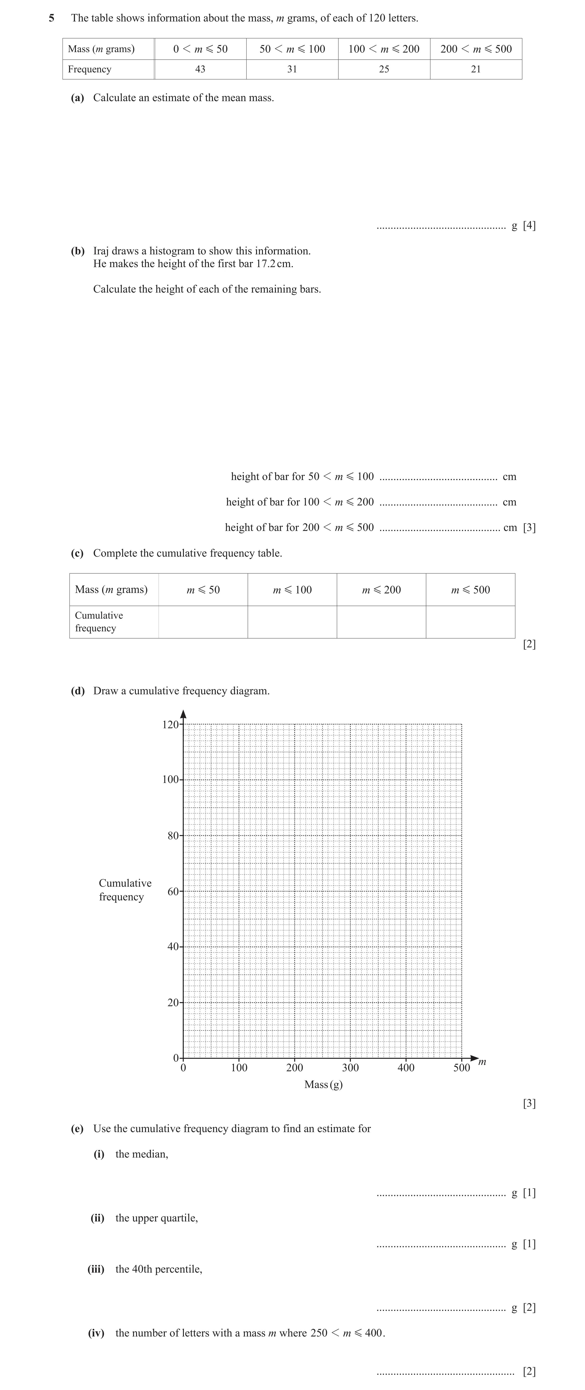
5 The table shows information about the mass, m grams, of each of 120 letters. Mass (m grams) 0 1 m G 50 50 1 m G 100 100 1 m G 200 200 1 m G 500 Frequency 43 31 25 21 (a) Calculate an estimate of the mean mass. … g [4] (b) Iraj draws a histogram to show this information. He makes the height of the first bar 17.2 cm. Calculate the height of each of the remaining bars. height of bar for 50 1 m G 100 … cm height of bar for 100 1 m G 200 … cm height of bar for 200 1 m G 500 … cm [3] (c) Complete the cumulative frequency table. Mass (m grams) m G 50 m G 100 m G 200 m G 500 Cumulative frequency [2] (d) Draw a cumulative frequency diagram. 120 100 80 Cumulative 60 frequency 40 20 0 m 0 100 200 300 400 500 Mass (g) [3] (e) Use the cumulative frequency diagram to find an estimate for (i) the median, … g [1] (ii) the upper quartile, … g [1] (iii) the 40th percentile, … g [2] (iv) the number of letters with a mass m where 250 1 m G 400 . … [2]
18 marks
Mark scheme: 5(a) 5 4 M1 for midpoints soi 121 or 120.8… or 120 6 M1 for use of ∑fx with x in correct interval including both boundaries but not if x is 50, 50, 100 and 300 M1 (dep on 2nd M1) for ∑fx ÷ 120 5(b) 12.4 5 1.4 3 B1 for each If 0 scored SC1 for fd’s [0.86,] 0.62, 0.25 and 0.07 oe 5(c) 43 74 99 120 2 B1 for 2 or 3 correct 5(d) Correct diagram 3 B1 for correct horizontal placement for 4 plots B1FT for correct vertical placement for 4 plots B1FT dep on at least B1 for reasonable increasing curve or polygon through their 4 points If 0 scored SC1 FT for 3 out of 4 points correctly plotted 5(e)(i) Strict FT their median reading 1 5(e)(ii) Strict FT their UQ reading 1 5(e)(iii) Strict FT their reading at 40th 2 B1 for 48 written or mark at cf = 48 on graph percentile 5(e)(iv) Strict FT their reading at 400 2 B1 for either correct reading at 250 or 400 – their reading at 250
This question in 0580/42 Feb/March 2022
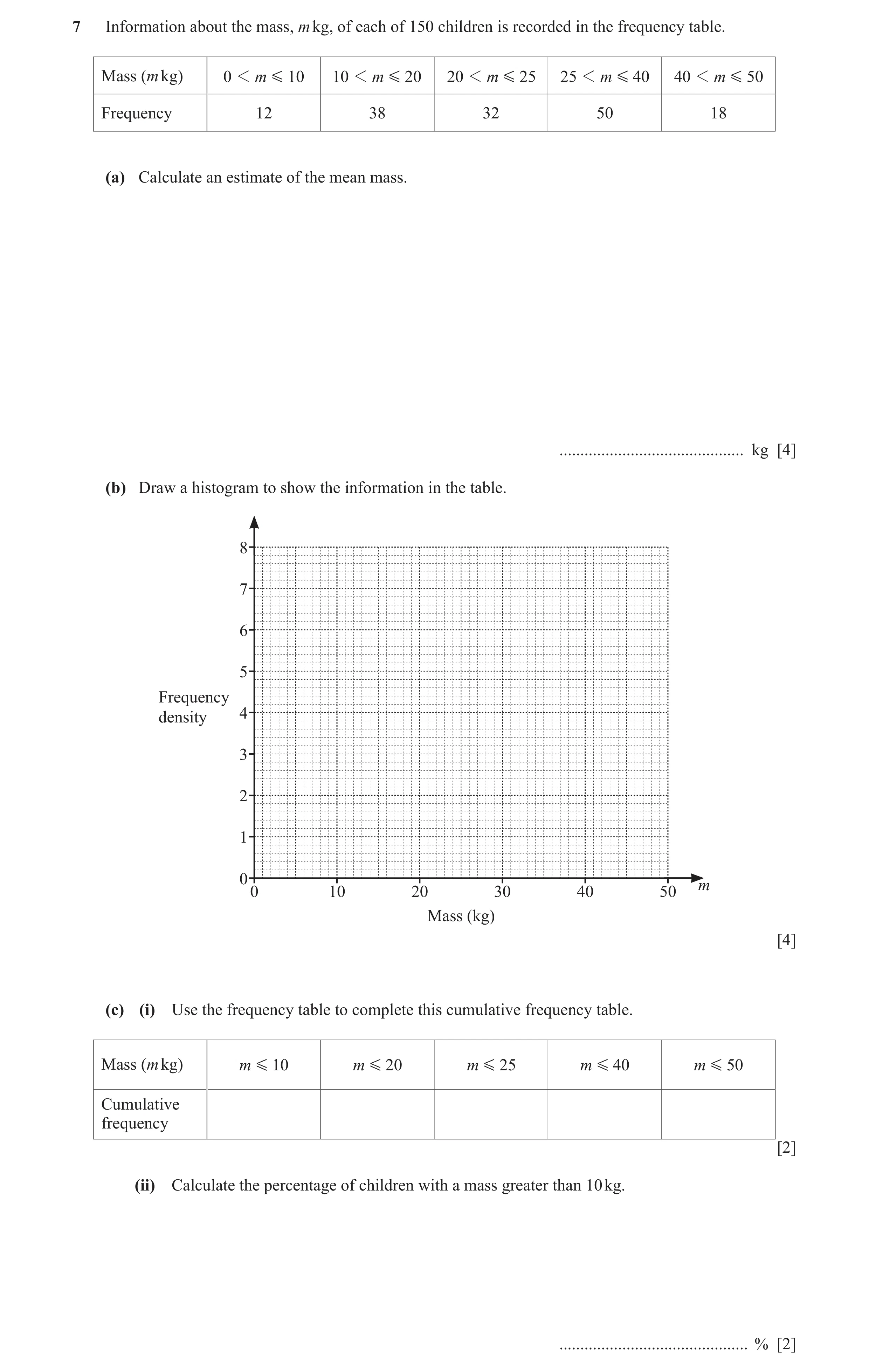
Q14 · Information about the mass, m kg, of each of 150 children is recorded in the frequency… 0580/42 May/June 2022
7 Information about the mass, m kg, of each of 150 children is recorded in the frequency table. Mass (m kg) 0 1 m G 10 10 1 m G 20 20 1 m G 25 25 1 m G 40 40 1 m G 50 Frequency 12 38 32 50 18 (a) Calculate an estimate of the mean mass. … kg [4] (b) Draw a histogram to show the information in the table. 8 7 6 5 Frequency density 4 3 2 1 0 m 0 10 20 30 40 50 Mass (kg) [4] (c) (i) Use the frequency table to complete this cumulative frequency table. Mass (m kg) m G 10 m G 20 m G 25 m G 40 m G 50 Cumulative frequency [2] (ii) Calculate the percentage of children with a mass greater than 10 kg. … % [2]
12 marks
Mark scheme: 7(a) 25.2 or 25.23… 4 M1 for midpoints soi M1 for use of ∑fx with x in correct interval including both boundaries M1 (dep on 2nd M1) for ∑fx ÷ 150 7(b) 5 correct blocks 4 B3 for 4 correct blocks or B2 for 3 correct blocks or B1 for 2 correct blocks or block widths 10, 10, 5, 15, 10 If 0 scored SC1 for 4 correct frequency densities from 1.2, 3.8, 6.4, 3.33[3…] and 1.8 oe soi 7(c)(i) 12, 50, 82, 132, 150 2 B1 for 3 or 4 correct 7(c)(ii) 92 2 M1 for 150 −12 oe seen If 0 scored, SC1 for answer 8[%]
This question in 0580/42 May/June 2022
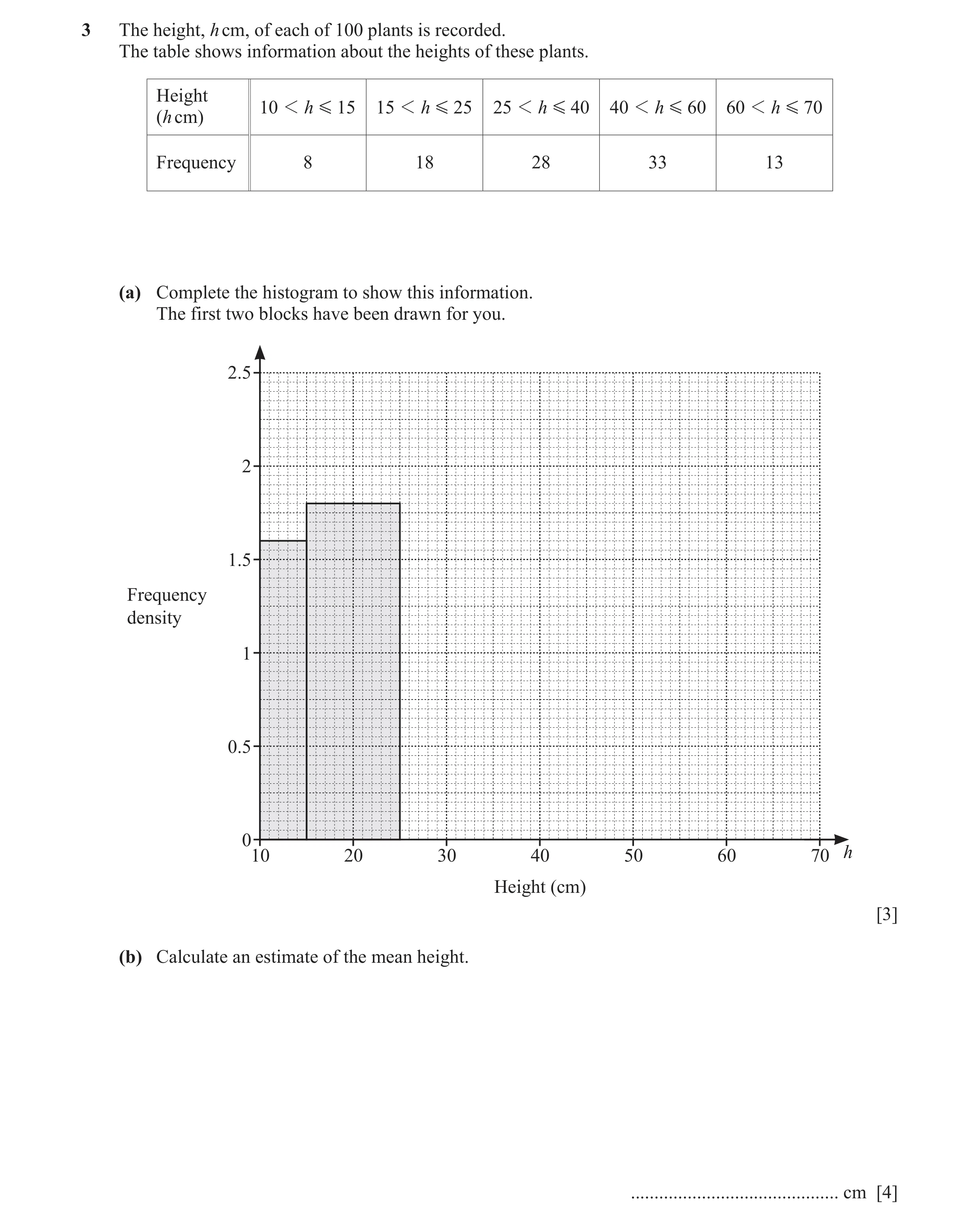
Q15 · The height, h cm, of each of 100 plants is recorded 0580/43 Oct/Nov 2022
3 The height, h cm, of each of 100 plants is recorded. The table shows information about the heights of these plants. Height 10 1 h G 15 15 1 h G 25 25 1 h G 40 40 1 h G 60 60 1 h G 70 (h cm) Frequency 8 18 28 33 13 (a) Complete the histogram to show this information. The first two blocks have been drawn for you. 2.5 2 1.5 Frequency density 1 0.5 0 10 20 30 40 50 60 70 h Height (cm) [3] (b) Calculate an estimate of the mean height. … cm [4]
7 marks
Mark scheme: 3(a) Correct histogram 3 B1 for each correct block 28 33 13 If 0 scored, SC1 for two of , , or 1.87 or 1.866 to 15 20 10 1.867, 1.65, 1.3 3(b) 38.65 4 M1 for 12.5, 20, 32.5, 50, 65 soi M1 for fx where x is in the correct interval including boundaries M1dep for fx ÷100
This question in 0580/43 Oct/Nov 2022
Q16 · There are 160 people in a village 0580/41 May/June 2023
5 (a) There are 160 people in a village. The cumulative frequency diagram shows information about their ages. 160 140 120 100 Cumulative 80frequency 60 40 20 0 0 10 20 30 40 50 60 70 Age (years) (i) Find an estimate for (a) the median age … [1] (b) the lower quartile … [1] (c) the number of people who are 50 or more years of age … [2] (d) the 65th percentile. … [2] (ii) The youngest person in the village is 1 year old and the oldest is 70 years old. (a) Draw a box-and-whisker plot to show the distribution of ages in the village. 0 10 20 30 40 50 60 70 80 Age (years) [3] (b) Write down an estimate of the percentage of people in the village that are younger than the median age. … % [1] (b) The frequency table shows information about the age of each person in another village. Age (n years) 0 1 n G 20 20 1 n G 30 30 1 n G 50 50 1 n G 80 Frequency 52 37 24 60 On the grid, complete the histogram to show this information. The first block has been drawn for you. 4 3 Frequency 2density 1 0 n 0 10 20 30 40 50 60 70 80 Age (years) [3]
13 marks
Mark scheme: 5(a)(i)(a) 25 1 5(a)(i)(b) 17 to 18 1 5(a)(i)(c) 12 2 B1 for 148 seen 5(a)(i)(d) 30 2 B1 for 104 seen 5(a)(ii)(a) correct diagram or correct for 3 B1 for whiskers at 1 and at 70 their median and LQ B1 for with median and LQ at their (a)(i)(a) and (a)(i)(b) B1 for UQ at 34 Maximum 2 marks if diagram incorrect If 0 scored SC1 for their 5 correct ages plotted 5(a)(ii)(b) 50 1 5(b) correct histogram 3 B1 for each correct block width 10 height 3.7 width 20 height 1.2 width 30 height 2 If 0 scored SC1 for correct frequency densities 3.7, 1.2, 2 oe
This question in 0580/41 May/June 2023
Q17 · Use your cumulative frequency diagram to find an estimate of (a) the median … km/h [1]… 0580/43 May/June 2023
(ii) Use your cumulative frequency diagram to find an estimate of (a) the median … km/h [1] (b) the interquartile range … km/h [2] (c) the number of cars with a speed greater than 110 km/h. … [2] (b) The frequency table shows information about the mass of each of 50 trucks. Mass 2000 1 m G 2600 2600 1 m G 3500 3500 1 m G 5000 5000 1 m G 5700 (m kg) Frequency 12 15 16 7 (i) Calculate an estimate for the mean mass of the trucks. … kg [4] (ii) In a histogram showing this information, the height of the first block is 6 cm. Calculate the heights of the remaining three blocks. Height of block for 2600 1 m G 3500 … cm Height of block for 3500 1 m G 5000 … cm Height of block for 5000 1 m G 5700 … cm [3]
15 marks
Mark scheme: 6(a)(i) Correct curve 3 B1 for correct horizontal placement for 6 plots B1 for correct vertical placement for 6 plots B1 dep on at least B1 for reasonable increasing curve through their 6 points If 0 scored, SC1 for 4 out of 6 points correctly plotted 6(a)(ii)(a) 87 to 89.5 1 6(a)(ii)(b) 12.5 to 14 2 B1 for [LQ =] 80.5 to 81.5 or [UQ =] 94 to 94.5 6(a)(ii)(c) Strict FT, 200 – their cumul freq reading 2 B1FT for correct cumul freq at 110 seen from their graph at 110 given to nearest or for non-integer answer integer 6(b)(i) 3576 4 M1 for midpoints soi M1 for use of fx where x is in the correct interval including boundaries M1 (dep on 2nd M1) for fx ÷ 50 6(b)(ii) 5 3.2 3 3 B1 for each If 0 scored, SC1 for 3 frequency densities 12 15 16 7 , , , seen oe to 3sf 600 900 1500 700 or better or multiplier 3 or 300
This question in 0580/43 May/June 2023
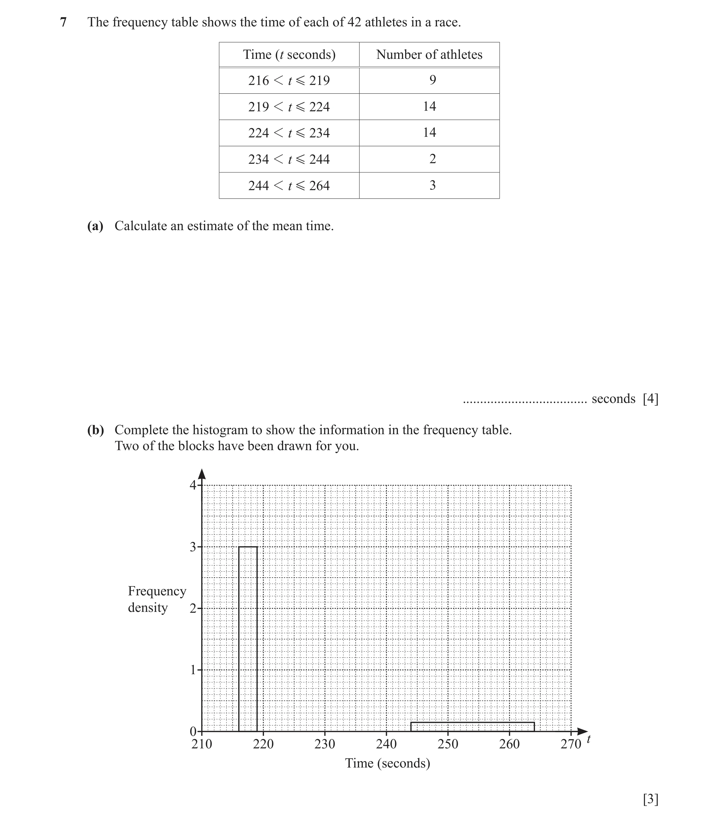
Q18 · The frequency table shows the time of each of 42 athletes in a race 0580/41 Oct/Nov 2023
7 The frequency table shows the time of each of 42 athletes in a race. Time (t seconds) Number of athletes 216 1 t G 219 9 219 1 t G 224 14 224 1 t G 234 14 234 1 t G 244 2 244 1 t G 264 3 (a) Calculate an estimate of the mean time. … seconds [4] (b) Complete the histogram to show the information in the frequency table. Two of the blocks have been drawn for you. 4 3 Frequency density 2 1 0 t 210 220 230 240 250 260 270 Time (seconds) [3]
7 marks
Mark scheme: 7(a) 226 nfww or 226.2 to 226.3[0] 4 M1 for mid-points soi nfww (217.5, 221.5, 229, 239, 254) M1 for use of fm with m in correct interval including both boundaries M1 (dep on 2nd M1) for fm (9 + 14 + 14 + 2 + 3) 7(b) Blocks with heights 2.8, 1.4, 0.2 3 B1 for each correct block and with correct widths If 0 scored, SC1 for two correct frequency densities soi
This question in 0580/41 Oct/Nov 2023
Q19 · Indira records the time taken for workers in her company to travel to work 0580/43 Oct/Nov 2023
5 Indira records the time taken for workers in her company to travel to work. The table and the histogram each show part of this information. Time (t minutes) 0 1 t G 10 10 1 t G 25 25 1 t G 40 40 1 t G 60 60 1 t G 80 Frequency 57 38 12 4 3 Frequency 2 density 1 0 t 0 10 20 30 40 50 60 70 80 Time (minutes) (a) Complete the table and the histogram. [5] (b) Calculate an estimate of the mean time. … min [4] (c) Rashid says: ‘The longest time that any of these workers take to travel to work is 80 minutes.’ Give a reason why Rashid may be wrong. … … [1] (d) Indira picks three workers at random from those who take longer than 25 minutes to travel to work. Calculate the probability that one worker takes 60 minutes or less and the other two each take more than 60 minutes. … [4]
14 marks
Mark scheme: 5(a) 28 and 45 on table B2 B1 for each Histogram correctly completed B3 B1 for each correct bar If 0 scored, SC1 for two of FD’s 3.8, 1.9 or 0.6 oe soi 5(b) 30.7 or 30.66 to 30.67 4 M1 for midpoints soi M1 for use of ∑fh with h in correct interval including both boundaries M1 (dep on 2nd M1) for ∑fh ÷ (their 28 + their 45 + 57 + 38 + 12) 5(c) Exact values are not known oe 1 5(d) 1254 4 M3 for oe 39 697 38 + 57 12 11 N oe 57 + 38 + 12 56 + 38 + 12 56 + 38 + 11 where N = 1, 2 or 3 38 + 57 12 or M2 for and 57 + 38 + 12 56 + 38 + 12 12 11 or and oe seen 57 + 38 + 12 57 + 38 + 11 38 + 57 12 or M1 for or oe seen 57 + 38 + 12 57 + 38 + 12 41040 If 0 scored SC1 for answer or 0.0335… 1225043
This question in 0580/43 Oct/Nov 2023
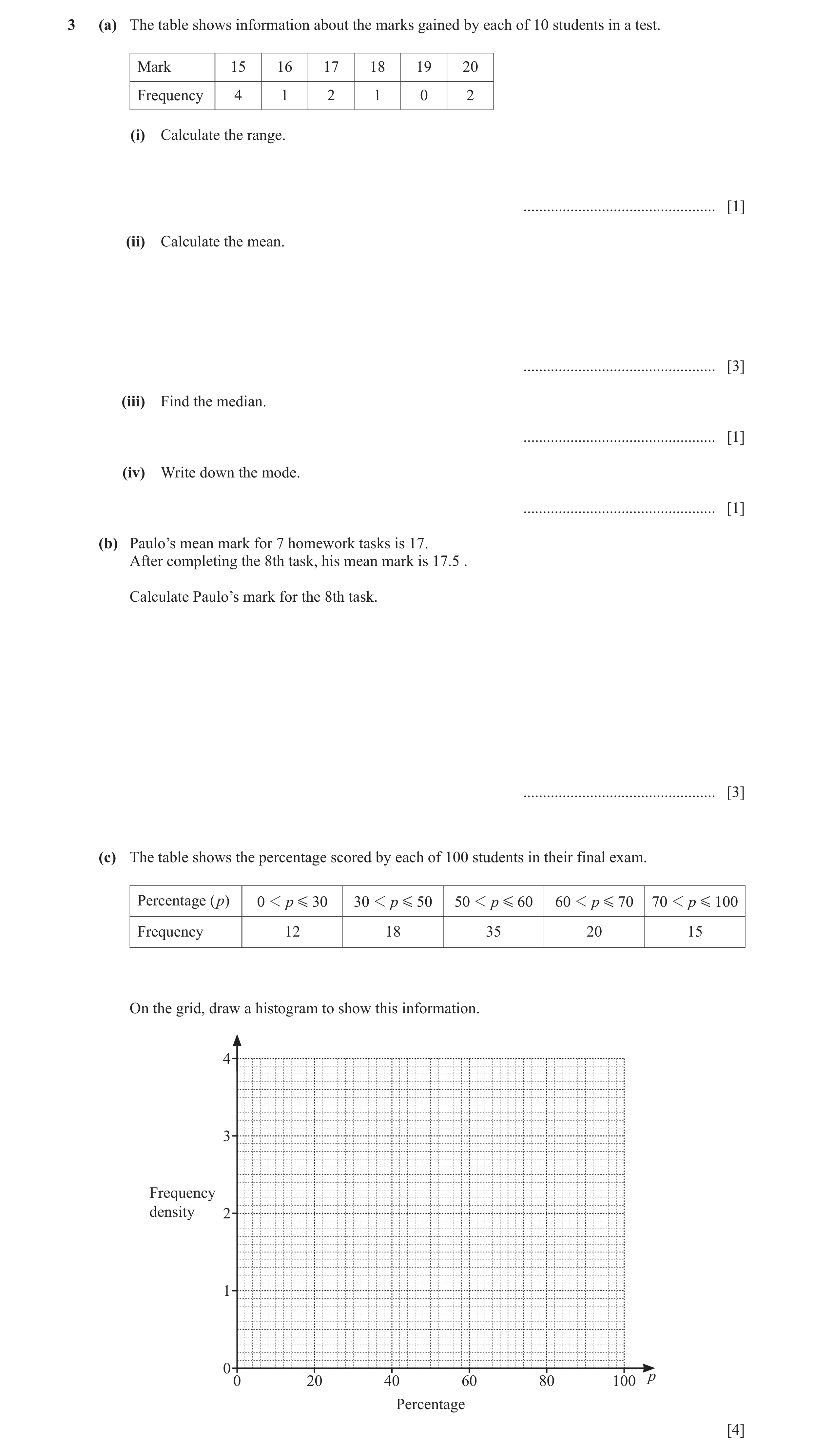
Q20 · The table shows information about the marks gained by each of 10 students in a test 0580/42 Feb/March 2024
3 (a) The table shows information about the marks gained by each of 10 students in a test. Mark 15 16 17 18 19 20 Frequency 4 1 2 1 0 2 (i) Calculate the range. … [1] (ii) Calculate the mean. … [3] (iii) Find the median. … [1] (iv) Write down the mode. … [1] (b) Paulo’s mean mark for 7 homework tasks is 17. After completing the 8th task, his mean mark is 17.5 . Calculate Paulo’s mark for the 8th task. … [3] (c) The table shows the percentage scored by each of 100 students in their final exam. Percentage ( p) 0 1 p G 30 30 1 p G 50 50 1 p G 60 60 1 p G 70 70 1 p G 100 Frequency 12 18 35 20 15 On the grid, draw a histogram to show this information. 4 3 Frequency density 2 1 0 p 0 20 40 60 80 100 Percentage [4]
13 marks
Mark scheme: 3(a)(i) 5 1 3(a)(ii) 16.8 3 M1 for 15 × 4 + 16 [× 1] + 17 × 2 + 18 [× 1 ] [+ 19 × 0] + 20 × 2 oe M1 dep on previous M1 for their Σfx ÷10 3(a)(iii) 16.5 1 3(a)(iv) 15 1 3(b) 21 3 M2 for 8 17.5 and 7 17 oe or M1 for 7 17 or 8 17.5 oe seen 3(c) 5 correct blocks, with correct widths, 4 B3 for 4 correct blocks heights 0.8cm, 1.8cm 7cm, 4cm, 1cm or B2 for 3 correct blocks or B1 for 2 correct blocks If 0 scored SC1 for correct frequency densities (0.4 0.9 3.5 2 0.5) soi
This question in 0580/42 Feb/March 2024
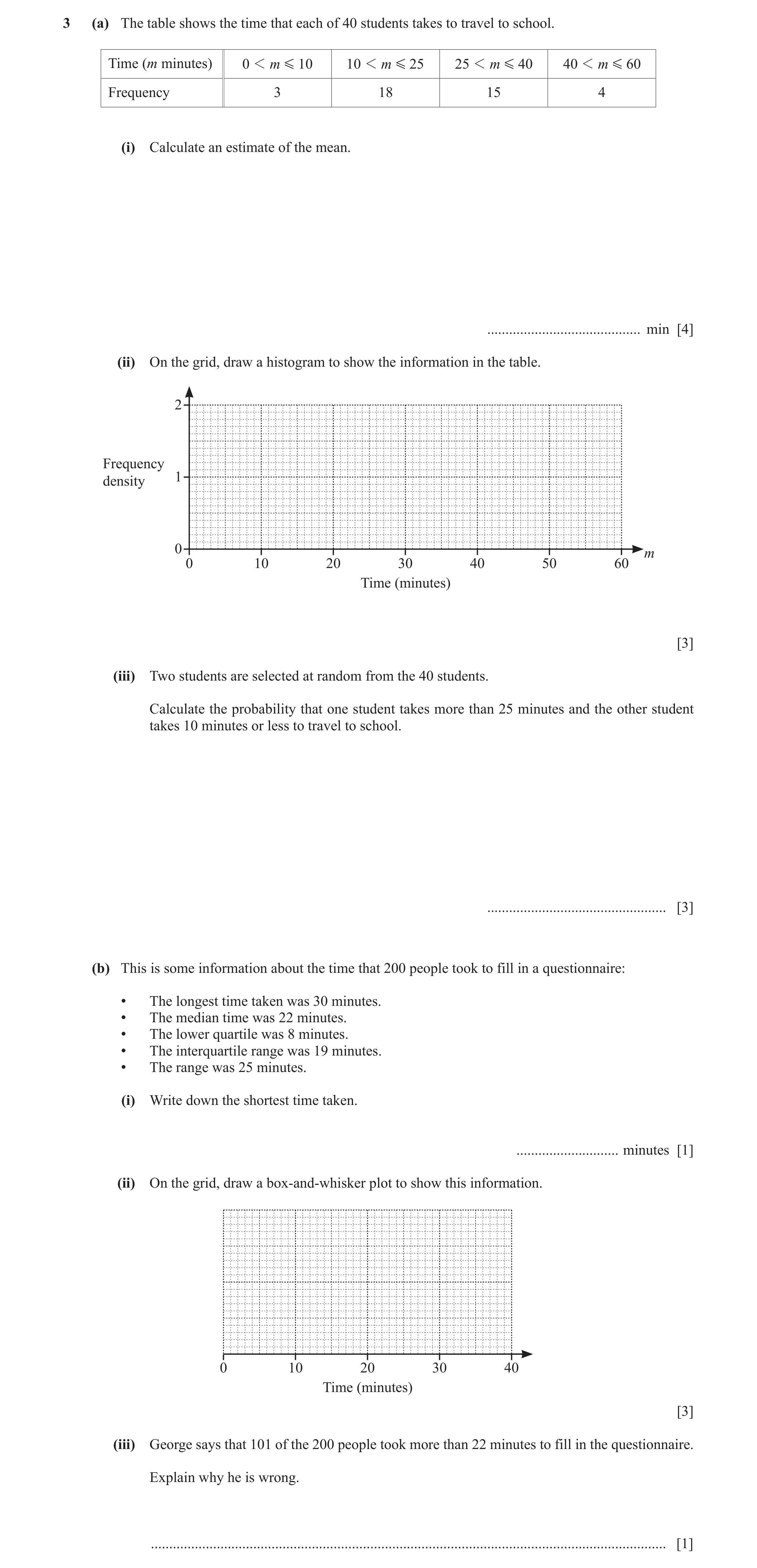
Q21 · The table shows the time that each of 40 students takes to travel to school 0580/42 May/June 2024
3 (a) The table shows the time that each of 40 students takes to travel to school. Time (m minutes) 0 1 m G 10 10 1 m G 25 25 1 m G 40 40 1 m G 60 Frequency 3 18 15 4 (i) Calculate an estimate of the mean. … min [4] (ii) On the grid, draw a histogram to show the information in the table. 2 Frequency 1 density 0 m 0 10 20 30 40 50 60 Time (minutes) [3] (iii) Two students are selected at random from the 40 students. Calculate the probability that one student takes more than 25 minutes and the other student takes 10 minutes or less to travel to school. … [3] (b) This is some information about the time that 200 people took to fill in a questionnaire: • The longest time taken was 30 minutes. • The median time was 22 minutes. • The lower quartile was 8 minutes. • The interquartile range was 19 minutes. • The range was 25 minutes. (i) Write down the shortest time taken. … minutes [1] (ii) On the grid, draw a box-and-whisker plot to show this information. 0 10 20 30 40 Time (minutes) [3] (iii) George says that 101 of the 200 people took more than 22 minutes to fill in the questionnaire. Explain why he is wrong. … [1]
15 marks
Mark scheme: 3(a)(i) 25.4375 4 M1 for mid-points soi (5, 17.5, 32.5, 50) M1 for use of fm with m in correct interval including both boundaries M1 for (dep on 2nd M1) for fm 40 3(a)(ii) correct histogram 3 B2 for 3 correct blocks or B1 for 2 correct blocks If 0 scored SC1 for 4 correct frequency densities 0.3, 1.2, 1, 0.2 oe soi 3(a)(iii) 19 3 oe 260 19 3 M2 for 2 oe 40 39 19 3 19 3 or M1 for any of , , , oe 40 40 39 39 seen 57 If 0 scored, SC1 for oe 800 3(b)(i) 5 1 3(b)(ii) 3 5 30 B2 for with LQ at 8 and median at 22 and 8 22 27 UQ at 27 and boxed or M1 for LQ at 8 and median at 22 Correct box plot or for UQ at 27 B1 for lowest = 5 and highest = 30 Max B1 if not box and whisker diagram 3(b)(iii) Correct explanation which states the 1 median is 22 and correct reference to 100 or 101 e.g. Median is 22 which is 50% of the people and 101 is more than 50% oe The median is 22 which is the 100th number (accept 100.5th number)
This question in 0580/42 May/June 2024
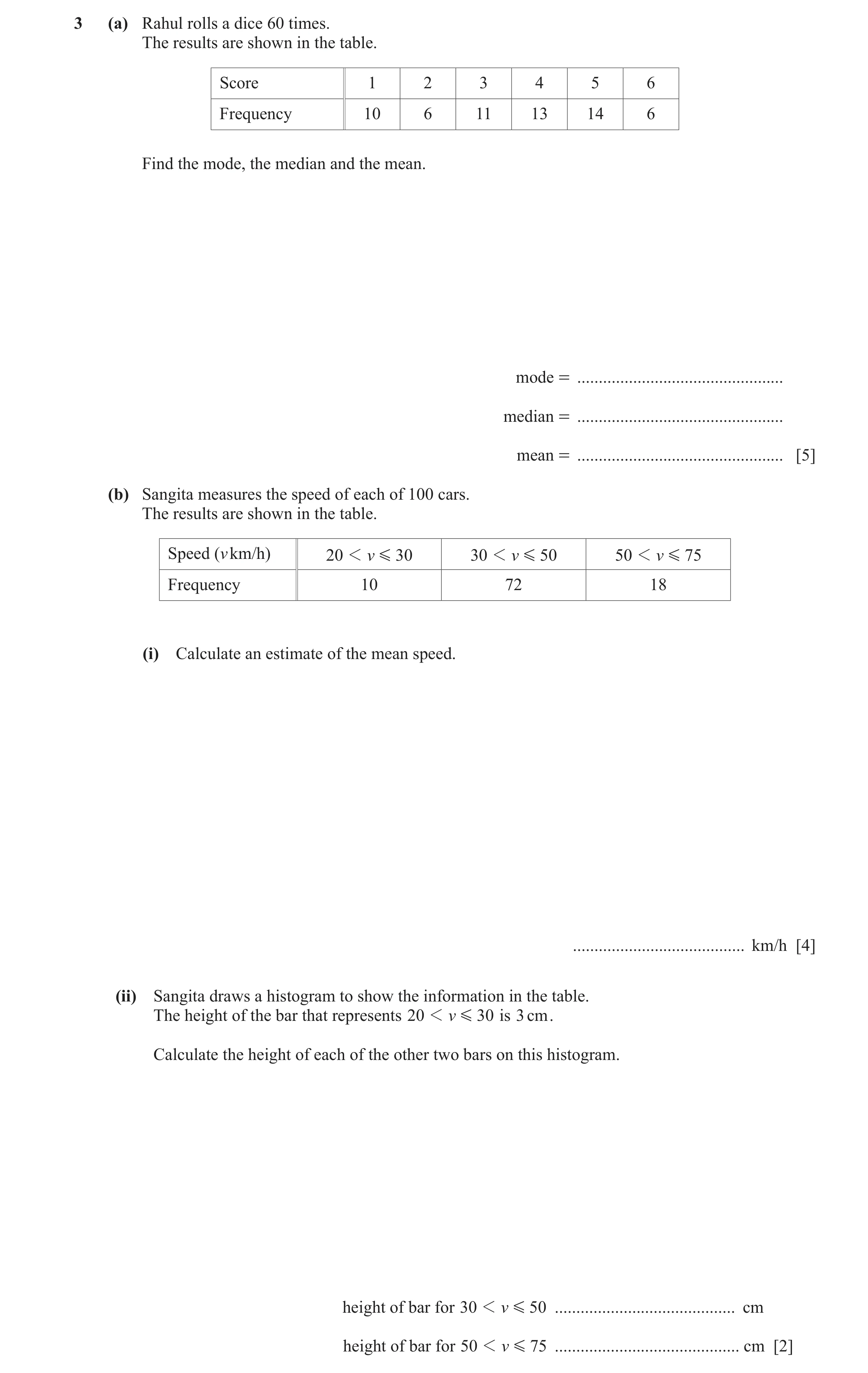
Q22 · Rahul rolls a dice 60 times 0580/43 May/June 2024
3 (a) Rahul rolls a dice 60 times. The results are shown in the table. Score 1 2 3 4 5 6 Frequency 10 6 11 13 14 6 Find the mode, the median and the mean. mode = … median = … mean = … [5] (b) Sangita measures the speed of each of 100 cars. The results are shown in the table. Speed (v km/h) 20 1 v G 30 30 1 v G 50 50 1 v G 75 Frequency 10 72 18 (i) Calculate an estimate of the mean speed. … km/h [4] (ii) Sangita draws a histogram to show the information in the table. The height of the bar that represents 20 1 v G 30 is 3 cm . Calculate the height of each of the other two bars on this histogram. height of bar for 30 1 v G 50 … cm height of bar for 50 1 v G 75 … cm [2]
11 marks
Mark scheme: 3(a) 5 B1 4 B1 3.55 3 M2 for (10 × 1 + 6 × 2 + 11 × 3 + 13 × 4 + 14 × 5 + 6 × 6) ÷ 60 oe or M1 for 10 × 1 + 6 × 2 + 11 × 3 + 13 × 4 + 14 × 5 + 6 × 6 oe 3(b)(i) 42.55 or 42.6 4 M1 for 25, 40, 62.5 soi M1 for fx with x values in correct intervals, including boundaries fx M1 dep on second M1 for 100 3(b)(ii) 10.8 2 B1 for each or for frequency densities 3.6 2.16 and 0.72 seen
This question in 0580/43 May/June 2024
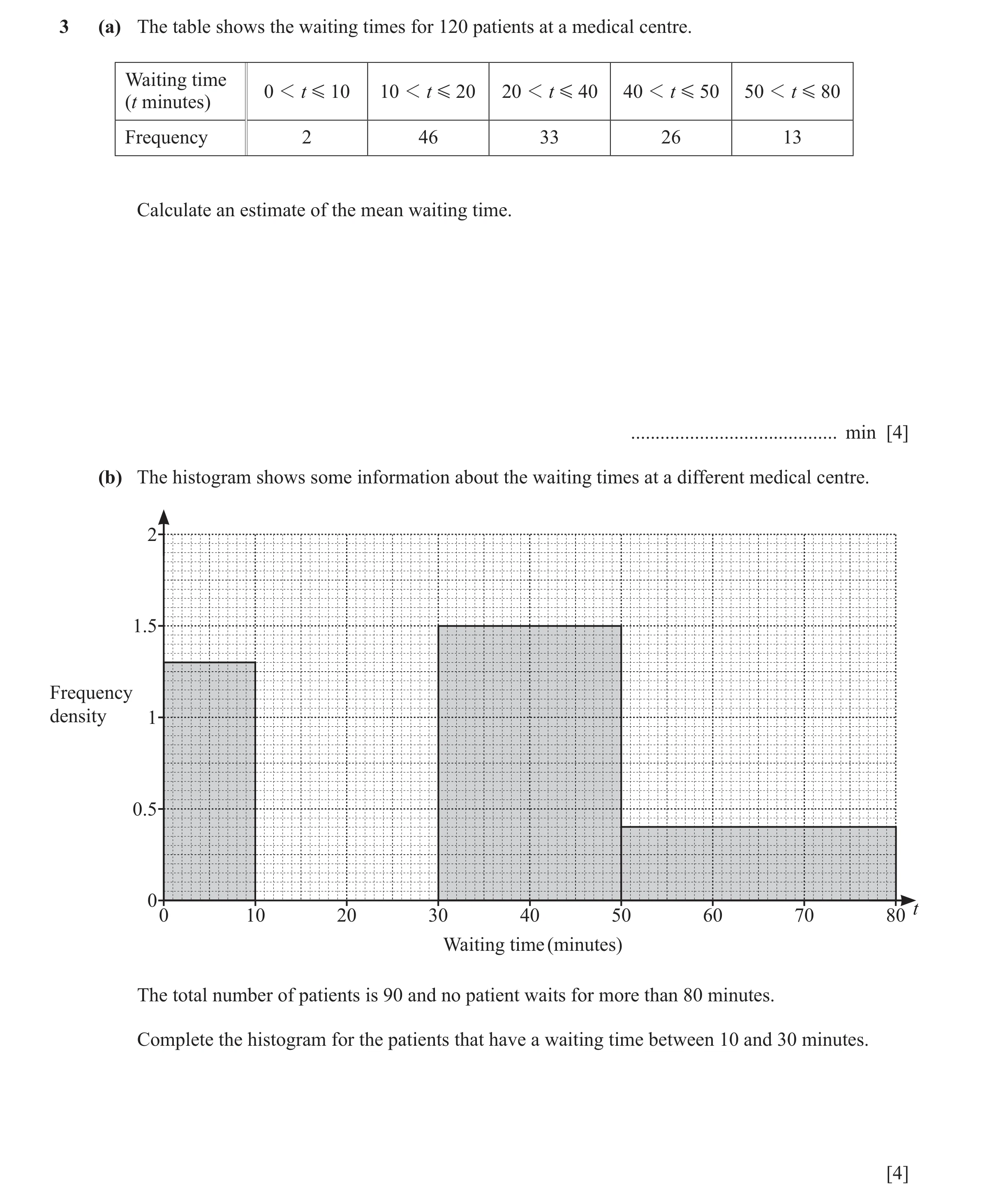
Q23 · The table shows the waiting times for 120 patients at a medical centre 0580/41 Oct/Nov 2024
3 (a) The table shows the waiting times for 120 patients at a medical centre. Waiting time 0 1 t G 10 10 1 t G 20 20 1 t G 40 40 1 t G 50 50 1 t G 80 (t minutes) Frequency 2 46 33 26 13 Calculate an estimate of the mean waiting time. … min [4] (b) The histogram shows some information about the waiting times at a different medical centre. 2 1.5 Frequency density 1 0.5 0 t 0 10 20 30 40 50 60 70 80 Waiting time (minutes) The total number of patients is 90 and no patient waits for more than 80 minutes. Complete the histogram for the patients that have a waiting time between 10 and 30 minutes. [4]
8 marks
Mark scheme: 3(a) 30.875 4 M1 for 5, 15, 30, 45, 65 soi M1 for fx M1 dep for their fx ÷ 120 dep on 2nd M1 3(b) Draws correct bar to height 1.75 4 B3 for [height = ] 1.75 OR M2 for [90 – ](10 × 1.3 + 20 × 1.5 + 30 × 0.4) oe or M1 for 10 × 1.3 or 20 × 1.5 or 30 × 0.4 M1dep for their frequency ÷ 20 dep on at least M1 After 0 scored SC1 for bar of correct width and height between 1.7 and 1.8
This question in 0580/41 Oct/Nov 2024
Q24 · The cumulative frequency diagram shows information about the distance travelled by each… 0580/42 Oct/Nov 2024
5 (a) The cumulative frequency diagram shows information about the distance travelled by each of 80 motorists in a month. 80 60 Cumulative 40 frequency 20 0 0 400 800 1200 1600 2000 2400 Distance (km) (i) Use the cumulative frequency diagram to find an estimate for (a) the median … km [1] (b) the interquartile range … km [2] (ii) One of these motorists is picked at random. Find the probability that this motorist travels more than 1800 km. … [2] (b) The distance around a racing track is 5.104 km. The time taken by a car to complete one lap of the track is 1 min 18 s. Calculate the average speed of the car. Give your answer in km/h. … km/h [3] (c) The top speed, v km/h, of each of 160 cars is recorded. The histogram shows this information. 2.0 1.5 Frequency 1.0 density 0.5 0 v 100 140 180 220 260 300 Top speed (km / h) (i) Show that there are 8 cars with a top speed in the interval 120 1 v G 160 . [1] (ii) Calculate an estimate of the mean top speed. You must show all your working. … km/h [6]
15 marks
Mark scheme: 5(a)(i)(a) 1480 1 5(a)(i)(b) 440 2 M1 for [UQ =] 1600 soi or [LQ =] 1160 soi 5(a)(ii) 8 2 oe M1 for 72 or 8 written 80 5(b) 236 or 235.5 to 235.6 3 5.104 M2 for 60 oe 1.3 5.104 or M1 for their time 5(c)(i) (160 – 120) 0.2 [ = 8] 1 with no errors seen 5(c)(ii) 22, 36, 64, 30 seen B2 B1 for 2 or 3 correct frequencies or M1 for three of 1.1 (180 – 160), 1.8 (200 – 180), 1.6 (240 – 200) and 0.5 (300 – 240) oe (8 × 140 + their22 × 170 M3 + their36 × 190 + their64 × 220 M1 for midpoints soi + their30 × 270) ÷ 160 M1 for fx , x in interval or boundary of interval M1 dep on second M1 for fx ÷ 160 211.75 B1
This question in 0580/42 Oct/Nov 2024
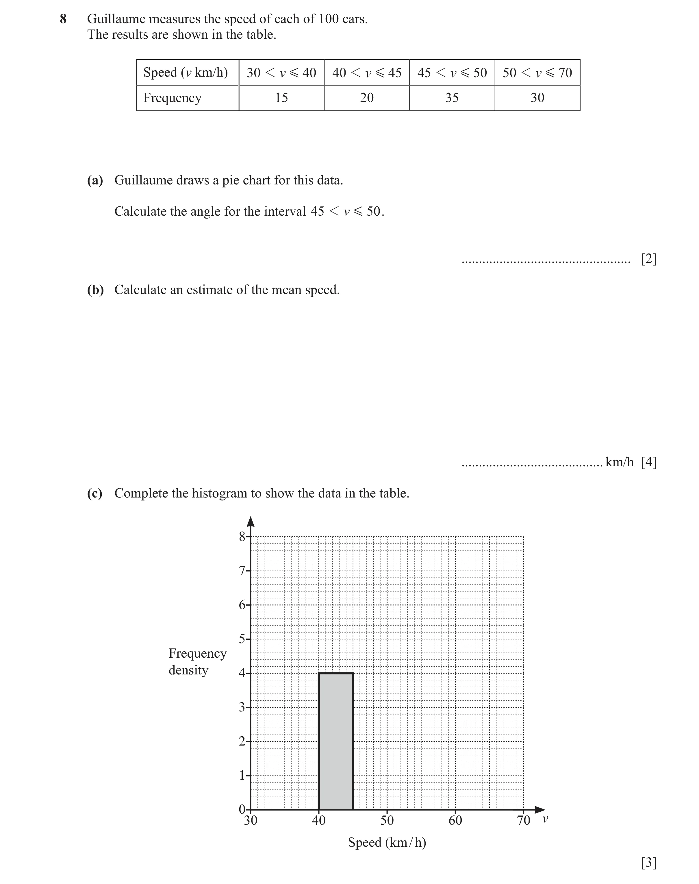
Q25 · Guillaume measures the speed of each of 100 cars 0580/43 Oct/Nov 2024
8 Guillaume measures the speed of each of 100 cars. The results are shown in the table. Speed (v km/h) 30 1 v G 4 0 40 1 v G 45 45 1 v G 50 50 1 v G 70 Frequency 15 20 35 30 (a) Guillaume draws a pie chart for this data. Calculate the angle for the interval 45 1 v G 50 . … [2] (b) Calculate an estimate of the mean speed. … km/h [4] (c) Complete the histogram to show the data in the table. 8 7 6 5 Frequency density 4 3 2 1 030 40 50 60 70 v Speed (km / h) [3]
9 marks
Mark scheme: 8(a) 126 2 35 M1 for 360 100 8(b) 48.375 4 M1 for mid-values 35, 42.5, 47.5, 60 soi M1 for 15 × 35 + 20 × 42.5 + 35 × 47.5 + 30 × 60 fx M1 dep dep on second M1 100 8(c) Correct histogram with correct widths 3 B1 for each column and heights 1.5, … 7, 1.5 If 0 scored, SC1 for freq. densities 1.5, ...7, 1.5 seen 15 35 30 or , , 10 5 20
This question in 0580/43 Oct/Nov 2024
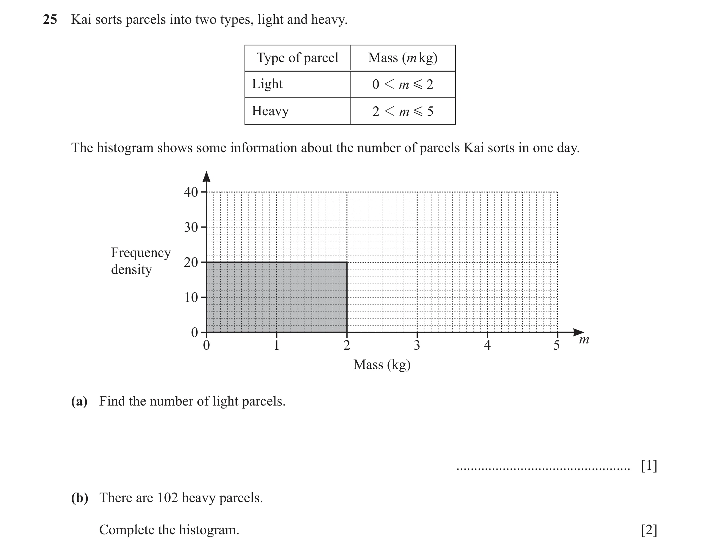
Q26 · Kai sorts parcels into two types, light and heavy 0580/41 Oct/Nov 2025
25 Kai sorts parcels into two types, light and heavy. Type of parcel Mass (m kg) Light 0 1 m G 2 Heavy 2 1 m G 5 The histogram shows some information about the number of parcels Kai sorts in one day. 40 30 Frequency 20 density 10 0 m 0 1 2 3 4 5 Mass (kg) (a) Find the number of light parcels. … [1] (b) There are 102 heavy parcels. Complete the histogram. [2]
3 marks
Mark scheme: 25(a) 40 1 25(b) Correct column, from 2 to 5 and 2 102 M1 for height 34 5 − 2
This question in 0580/41 Oct/Nov 2025
Q27 · The histogram shows information about the masses of some coconuts 0580/42 Oct/Nov 2025
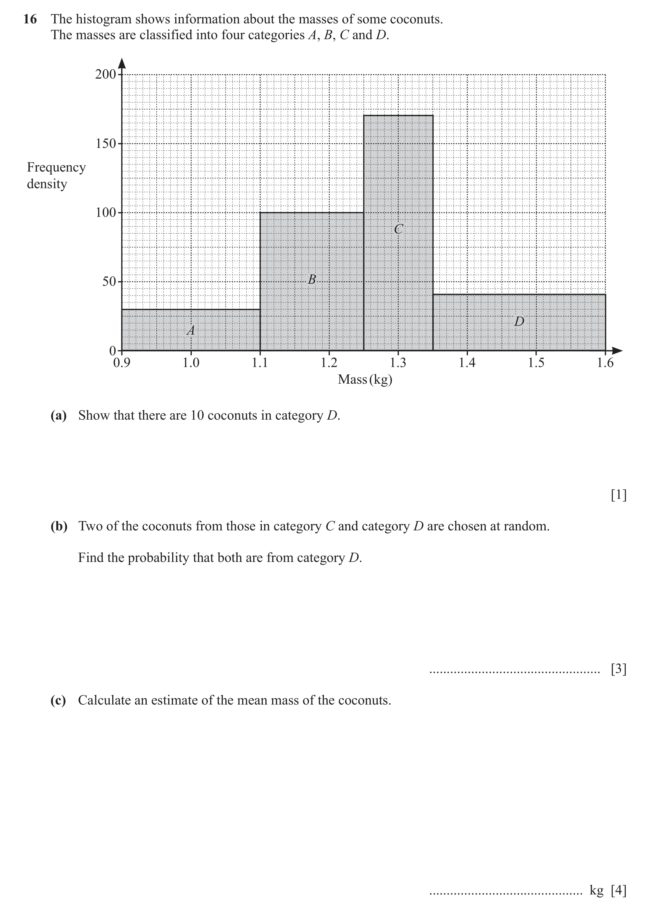
16 The histogram shows information about the masses of some coconuts. The masses are classified into four categories A, B, C and D. 200 150 Frequency density 100 C 50 B D A 0 0.9 1.0 1.1 1.2 1.3 1.4 1.5 1.6 Mass (kg) (a) Show that there are 10 coconuts in category D. [1] (b) Two of the coconuts from those in category C and category D are chosen at random. Find the probability that both are from category D. … [3] (c) Calculate an estimate of the mean mass of the coconuts. … kg [4]
8 marks
Mark scheme: 16(a) (1.6 – 1.35) oe × 40 [= 10] 1 16(b) 5 3 10 9 oe M2 for oe 39 10 + 170 0.1 9 + 170 0.1 10 9 9 10 or M1 for or or or oe 10 + 17 10 + 16 10 + 17 10 + 16 seen 10 9 or oe with k > 10 and an integer k k − 1 m m − 1 or oe with 0 < m < 27 and an integer 10 + 17 10 + 16 16(c) 1.26 or 1.259… nfww 4 M1 for frequencies 6, 15, 17 soi M1 for midpoints soi (1, 1.175, 1.3, 1.475) M1 for use of their fm their f with m in correct interval including both boundaries
This question in 0580/42 Oct/Nov 2025
Q28 · The table shows some information about the mass of each of 200 oranges 0580/43 Oct/Nov 2025
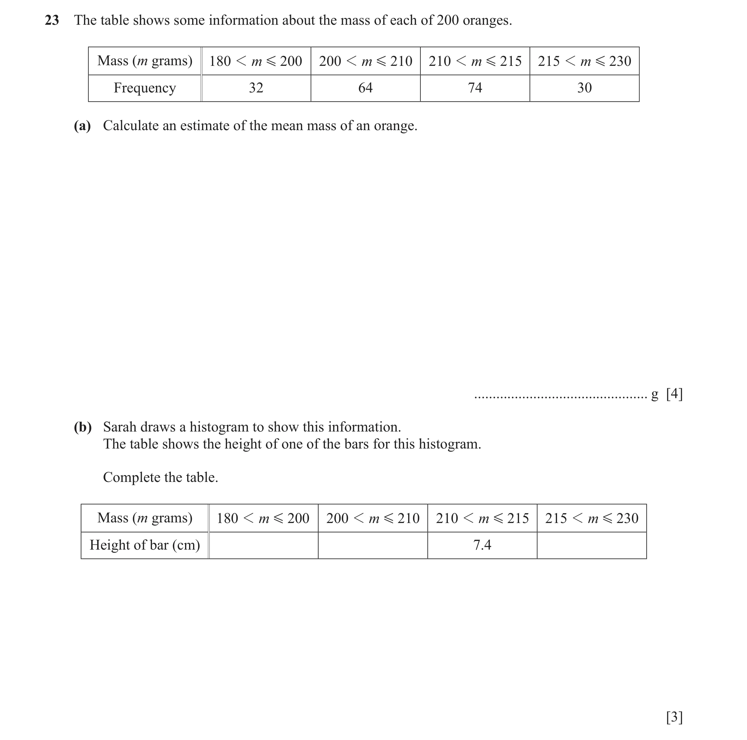
23 The table shows some information about the mass of each of 200 oranges. Mass (m grams) 180 1 m G 200 200 1 m G 2 10 210 1 m G 215 215 1 m G 230 Frequency 32 64 74 30 (a) Calculate an estimate of the mean mass of an orange. … g [4] (b) Sarah draws a histogram to show this information. The table shows the height of one of the bars for this histogram. Complete the table. Mass (m grams) 180 1 m G 200 200 1 m G 2 10 210 1 m G 215 215 1 m G 230 Height of bar (cm) 7.4 [3]
7 marks
Mark scheme: 23(a) 208 4 M1 for midpoints soi 190, 205, 212.5, 222.5 M1 for use of Σfx where x is in the correct interval including boundaries 190 × 32 + 205 × 64 + 212.5 × 74 + 222.5 × 30 M1 (dep on second M1) for Σfx ÷ 200 23(b) 0.8 3.2 1 3 B2 for two correct or B1 for one correct or M1 for three of 1.6, 6.4, 14.8 and 2 seen
This question in 0580/43 Oct/Nov 2025
 10 / 43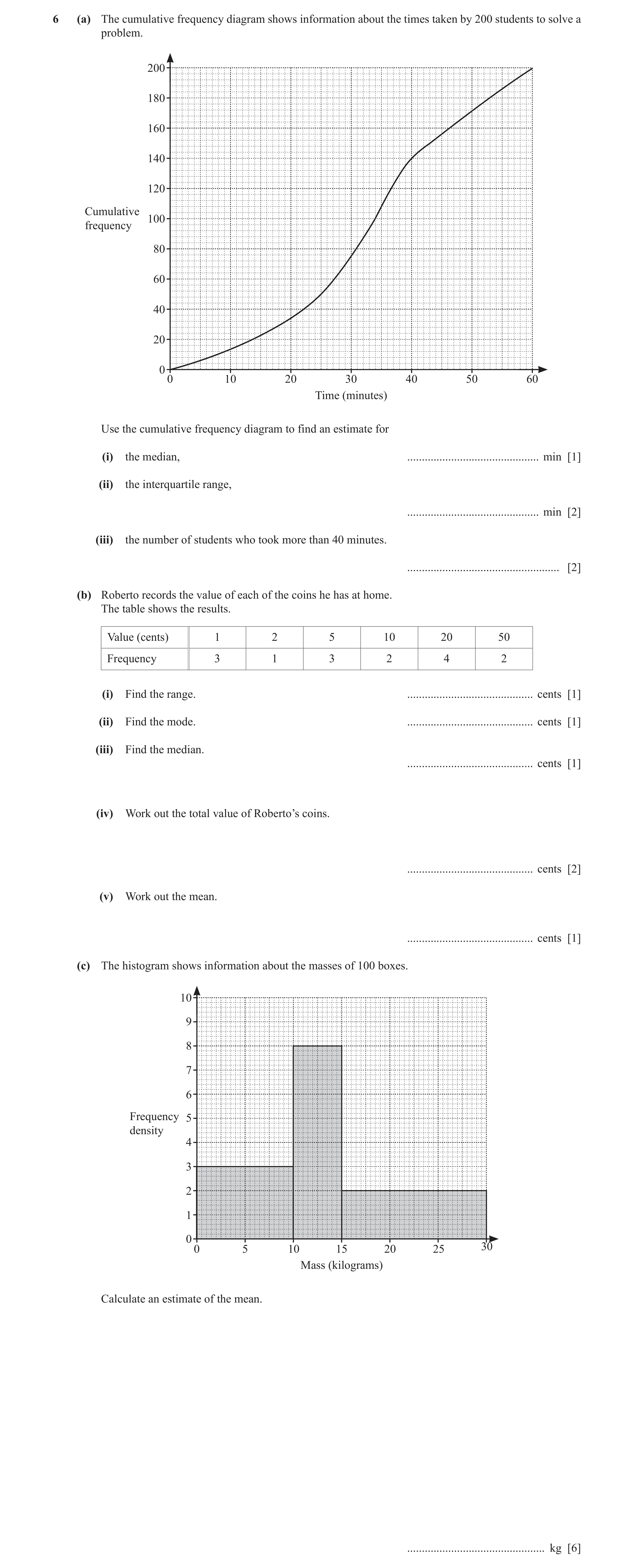
![Question 12: (a) Zoe’s test scores last term were 6 7 7 7 8 9 9 10 10. Find (i) the range, ................................................. [1] (ii) th…](https://img.pastlit.com/crops/3ef72f55-5a57-44e6-9d01-91338575f77e/q3.webp)
 25 / 43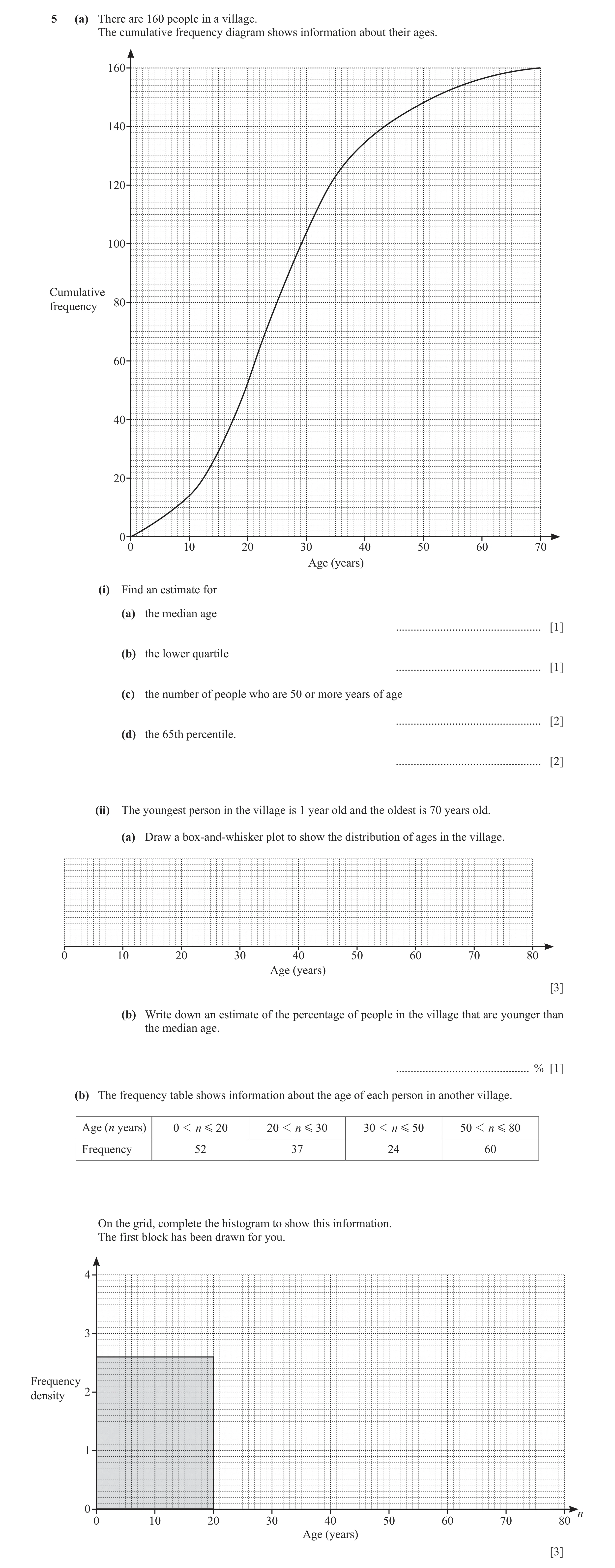
![Question 17: (ii) Use your cumulative frequency diagram to find an estimate of (a) the median ........................................ km/h [1] (b) the …](https://img.pastlit.com/crops/8f43649c-25cd-4a6e-9498-26bd158be84e/q6.webp)
 30 / 43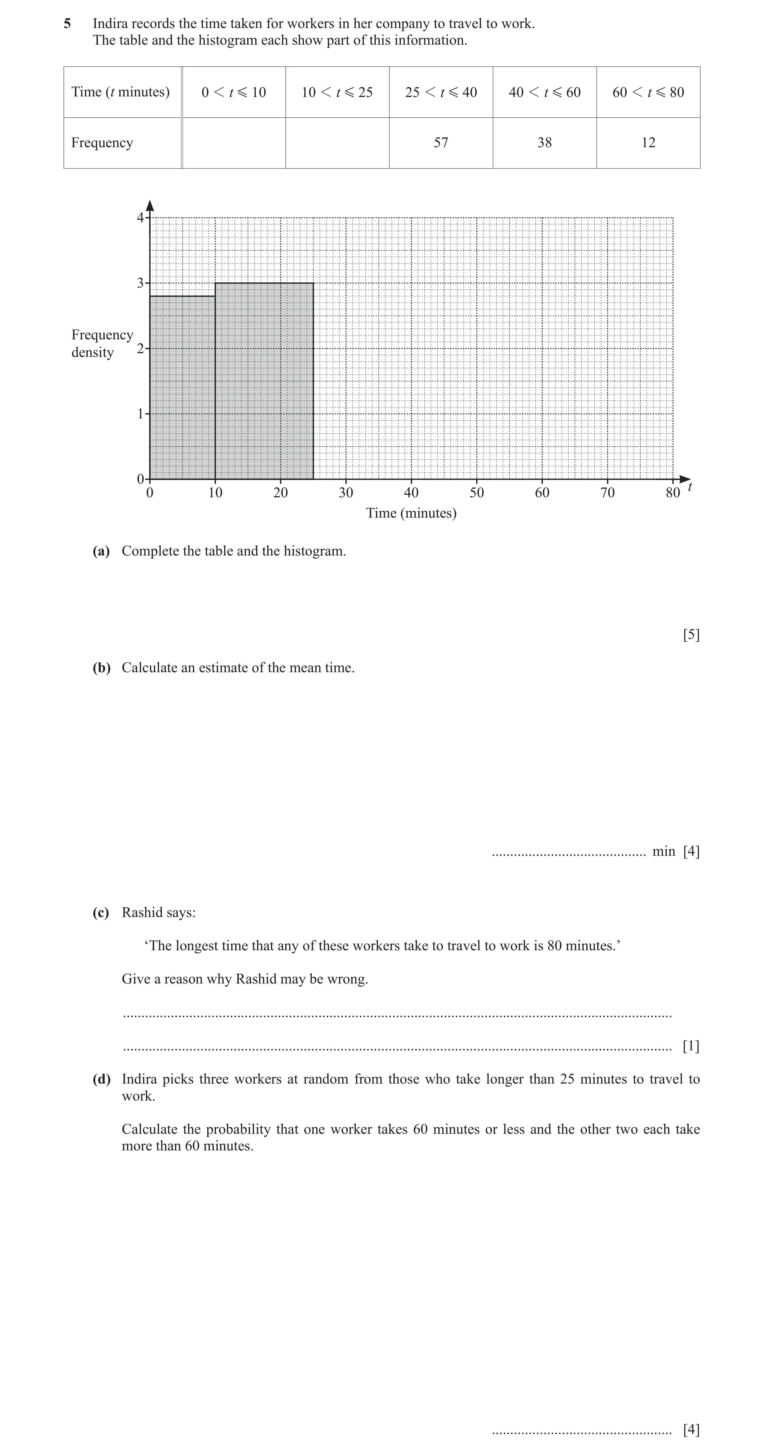
 37 / 43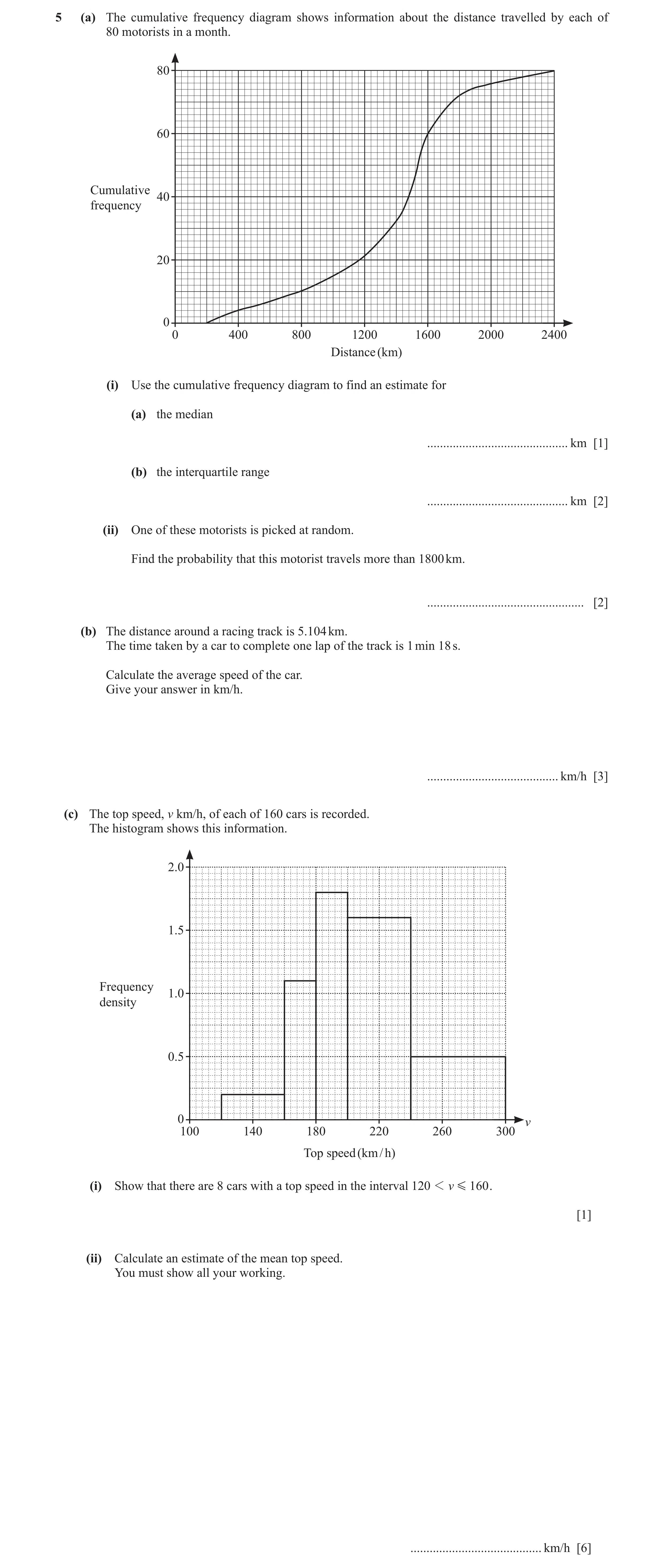
 40 / 43
 41 / 43
 42 / 43
 43 / 43
 13
13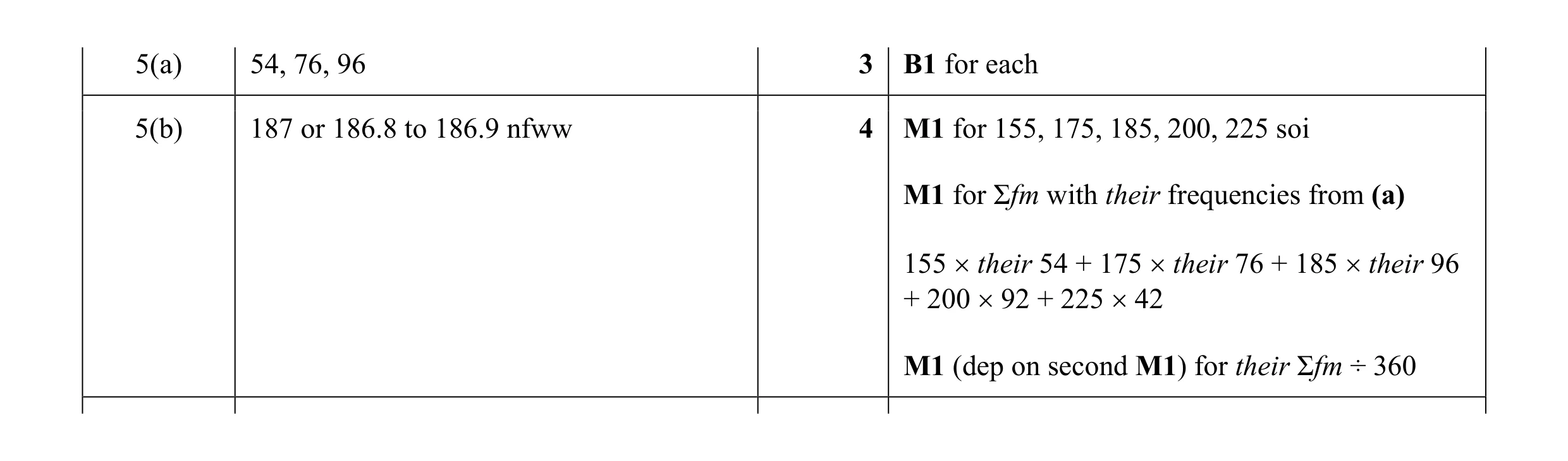 7
7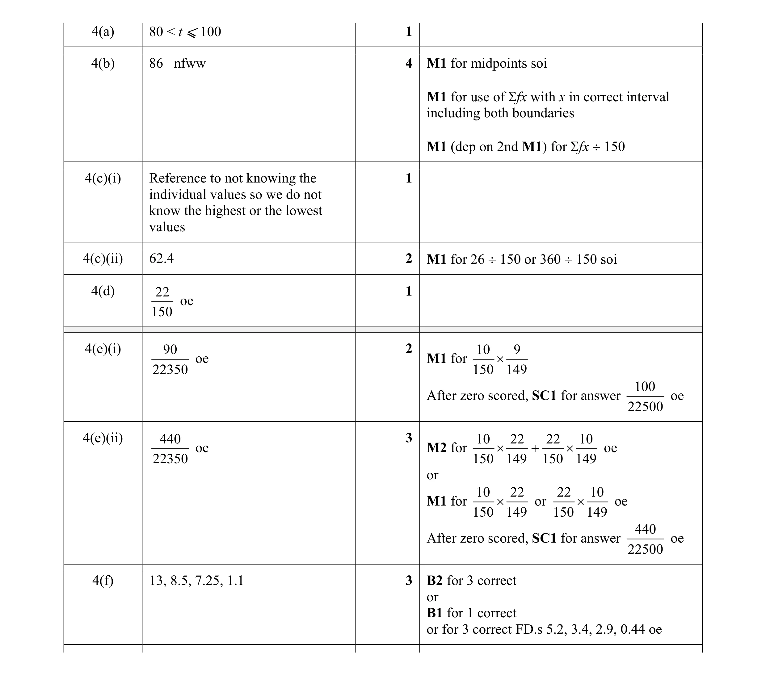 17
17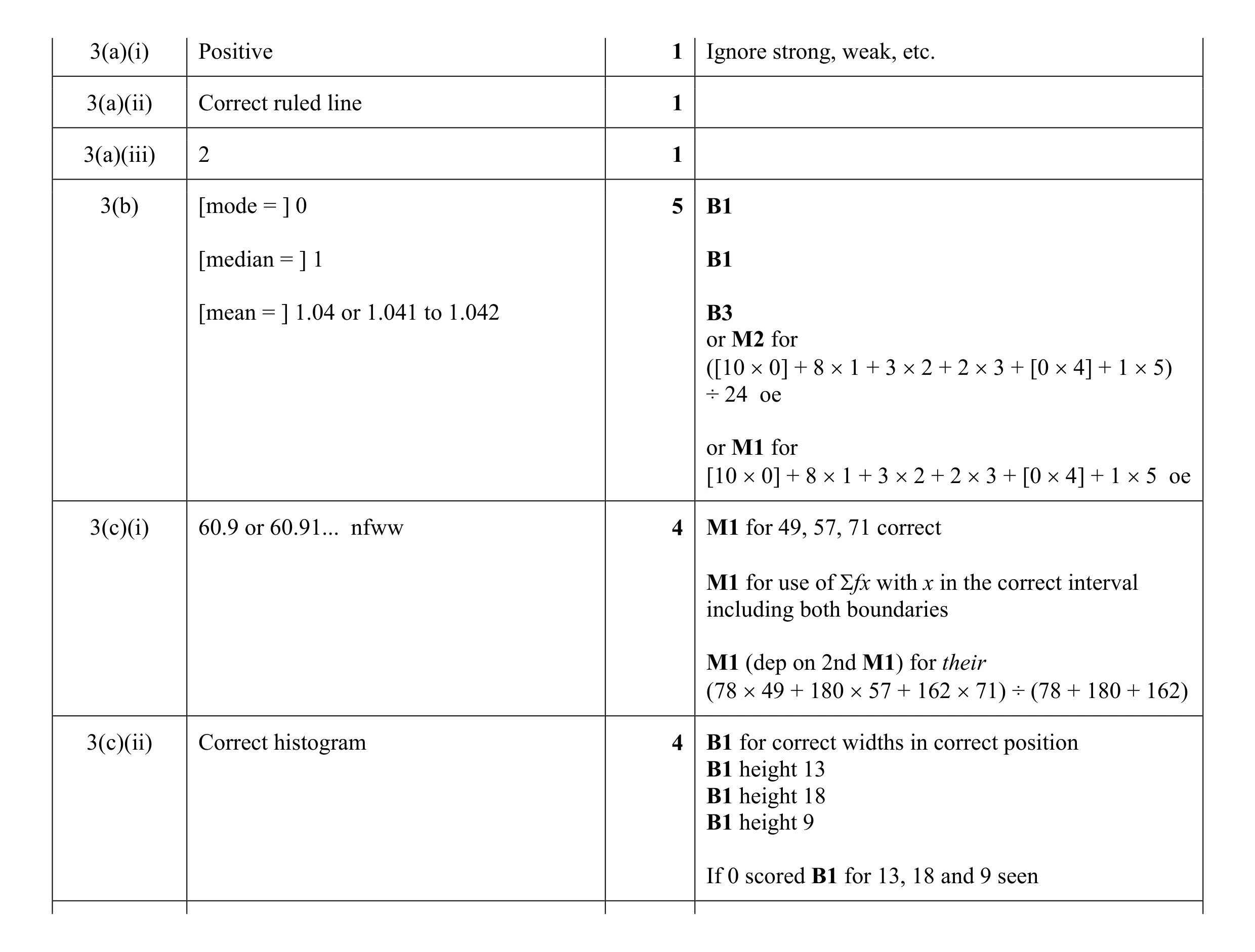 16
16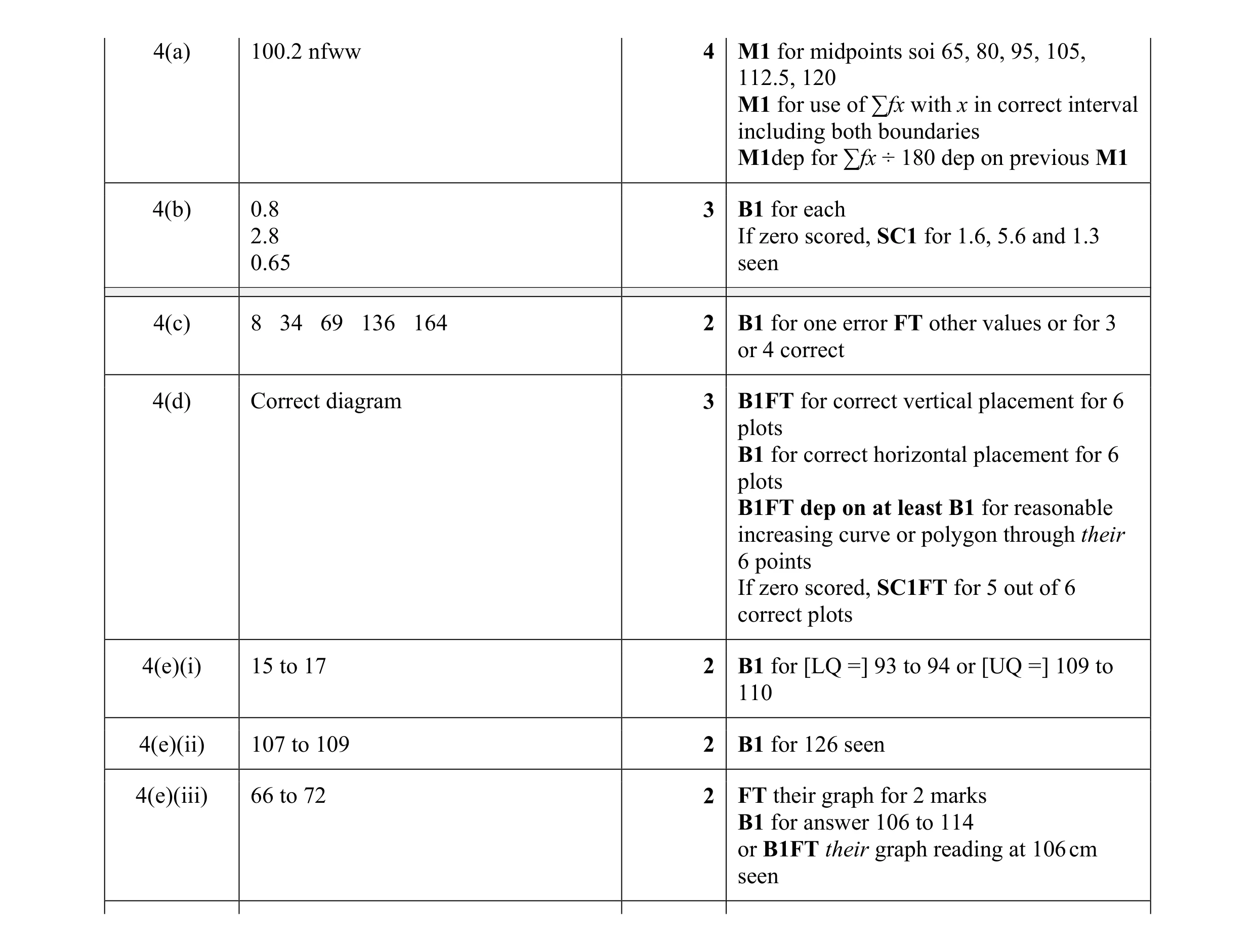 18
18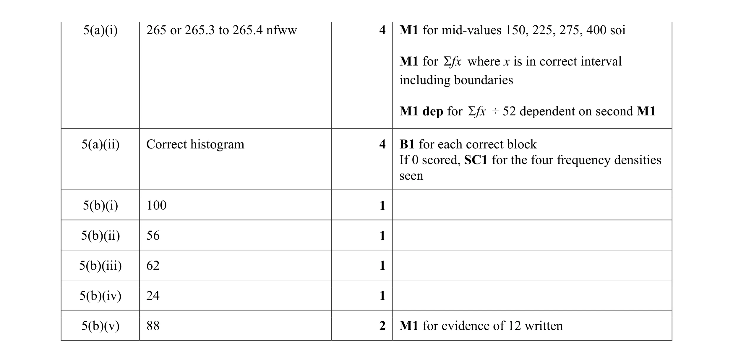 14
14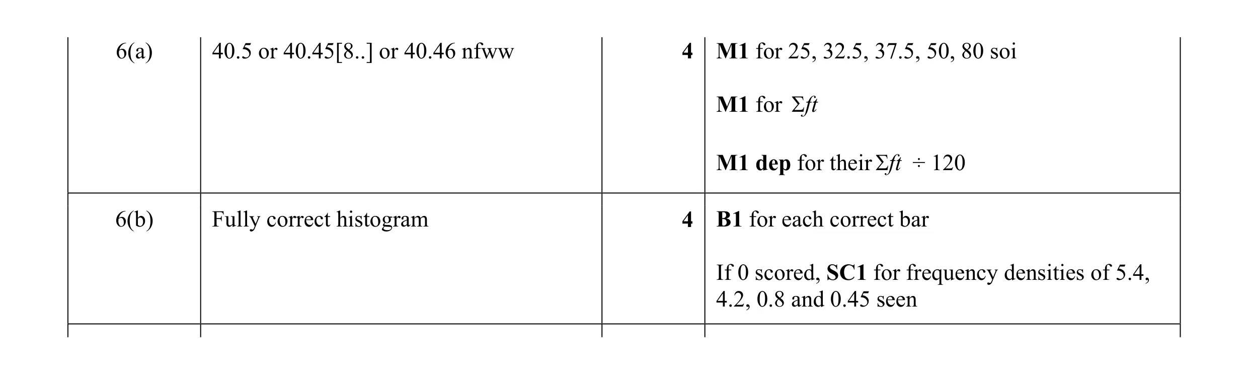 8
8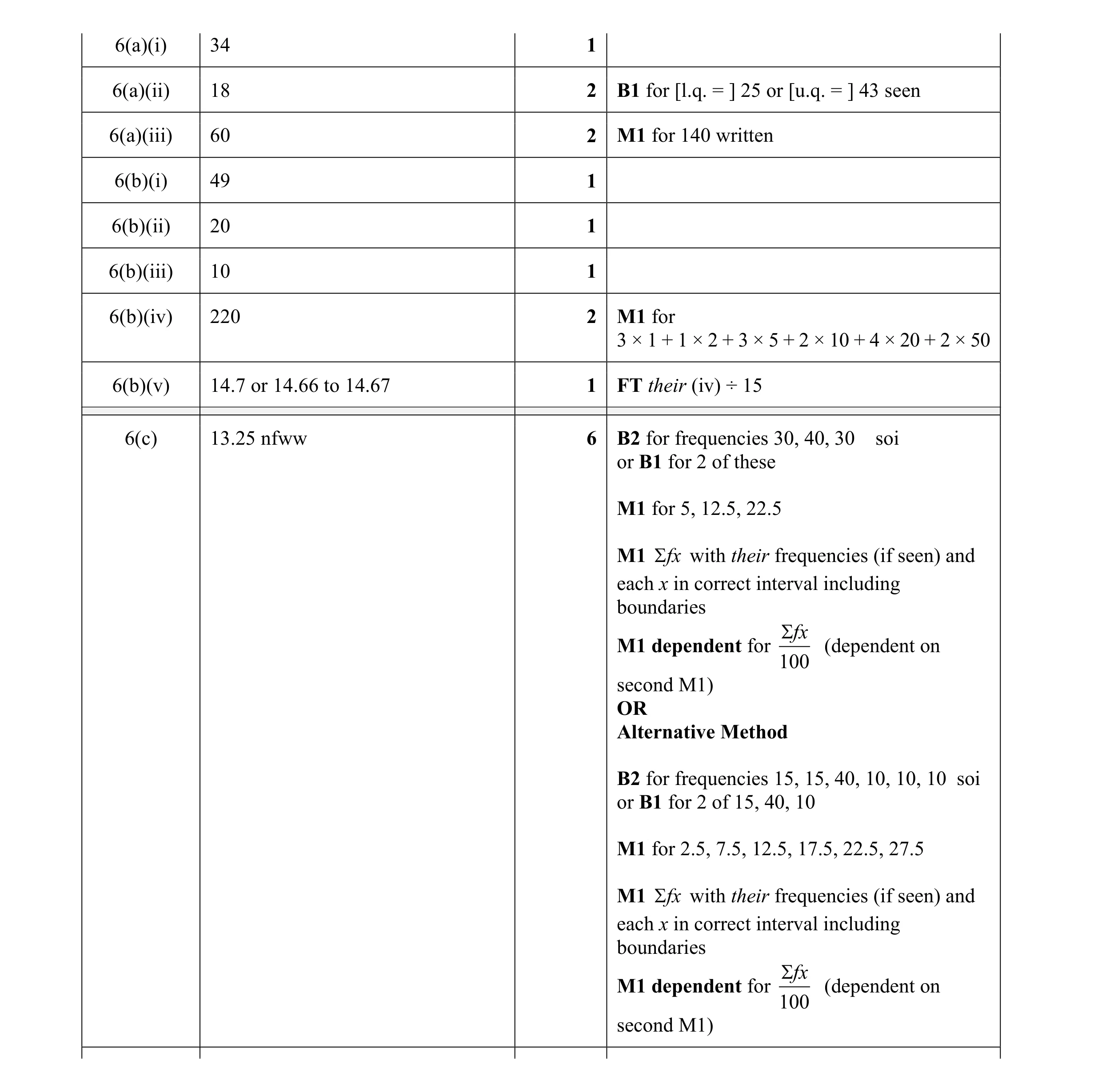 17
17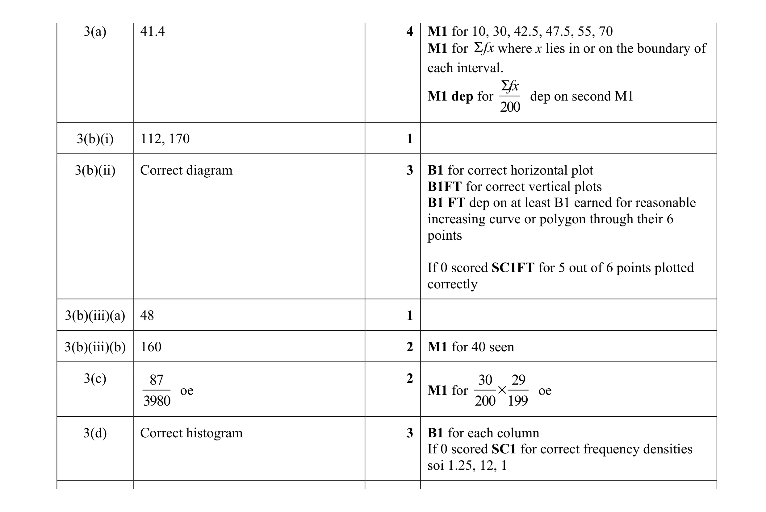 16
16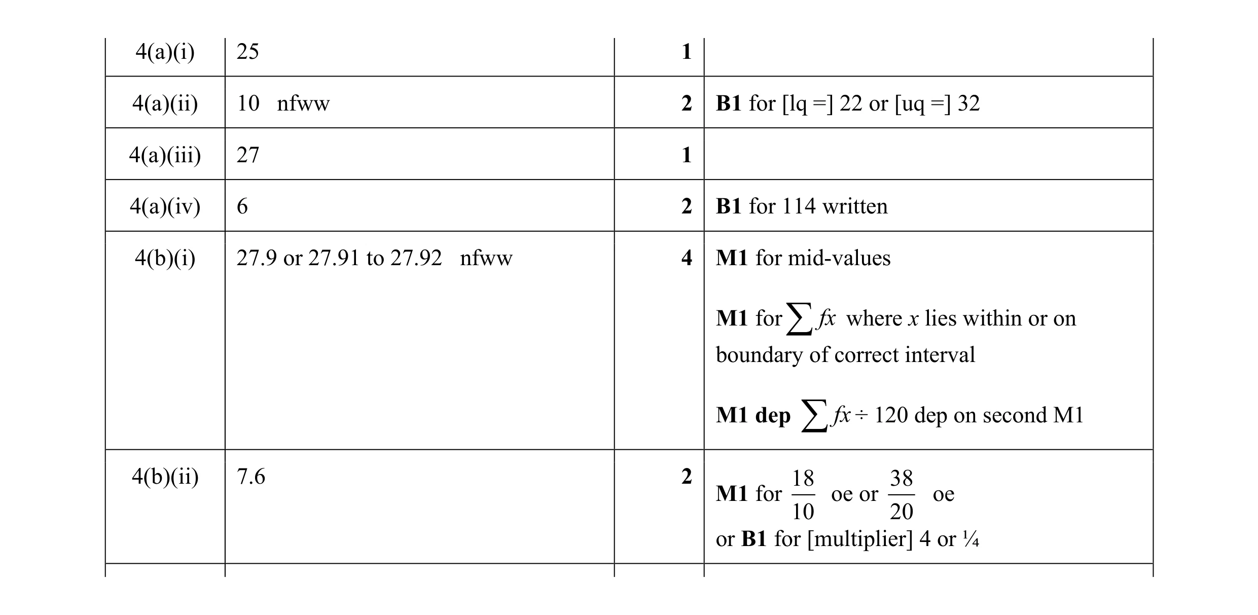 12
12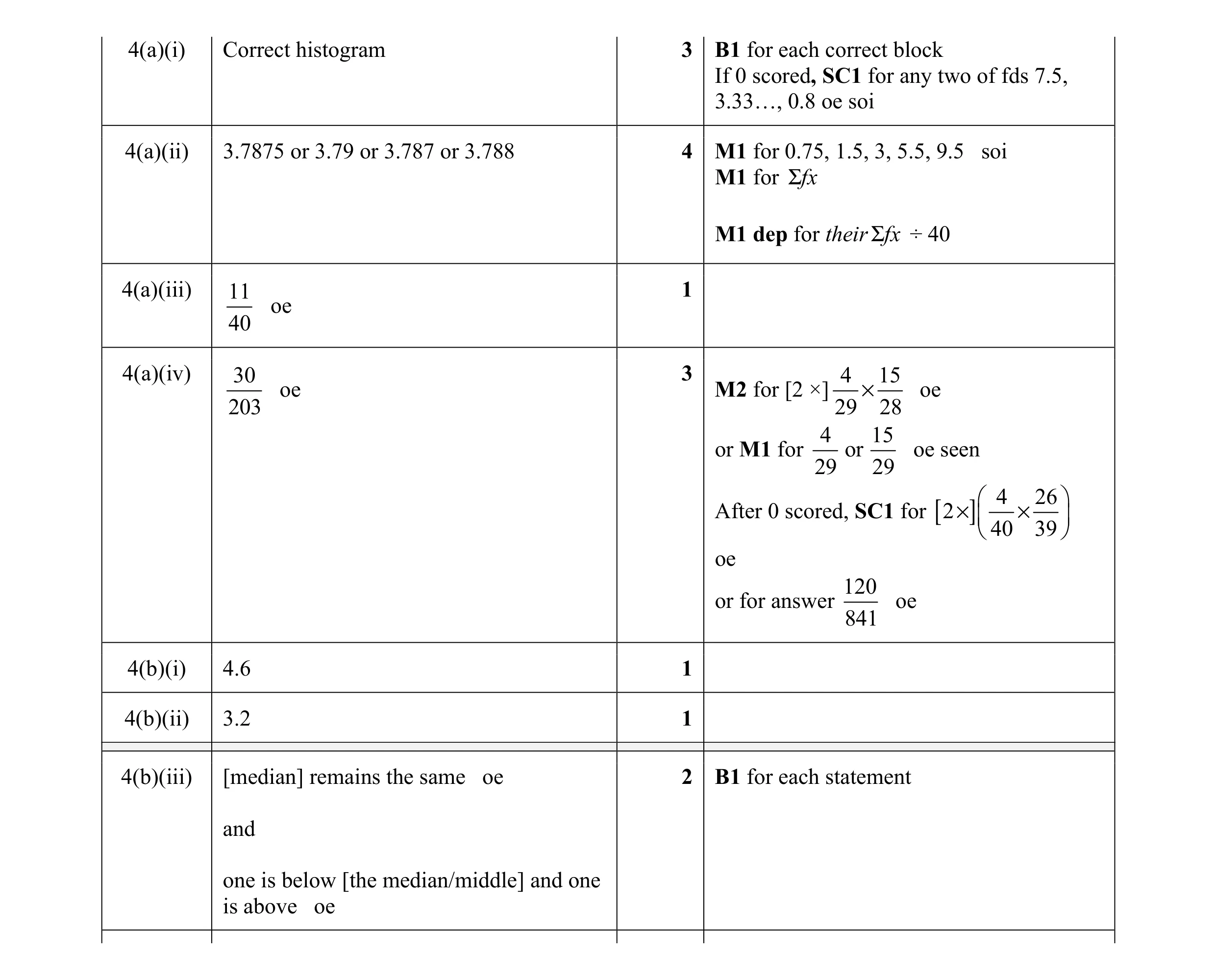 15
15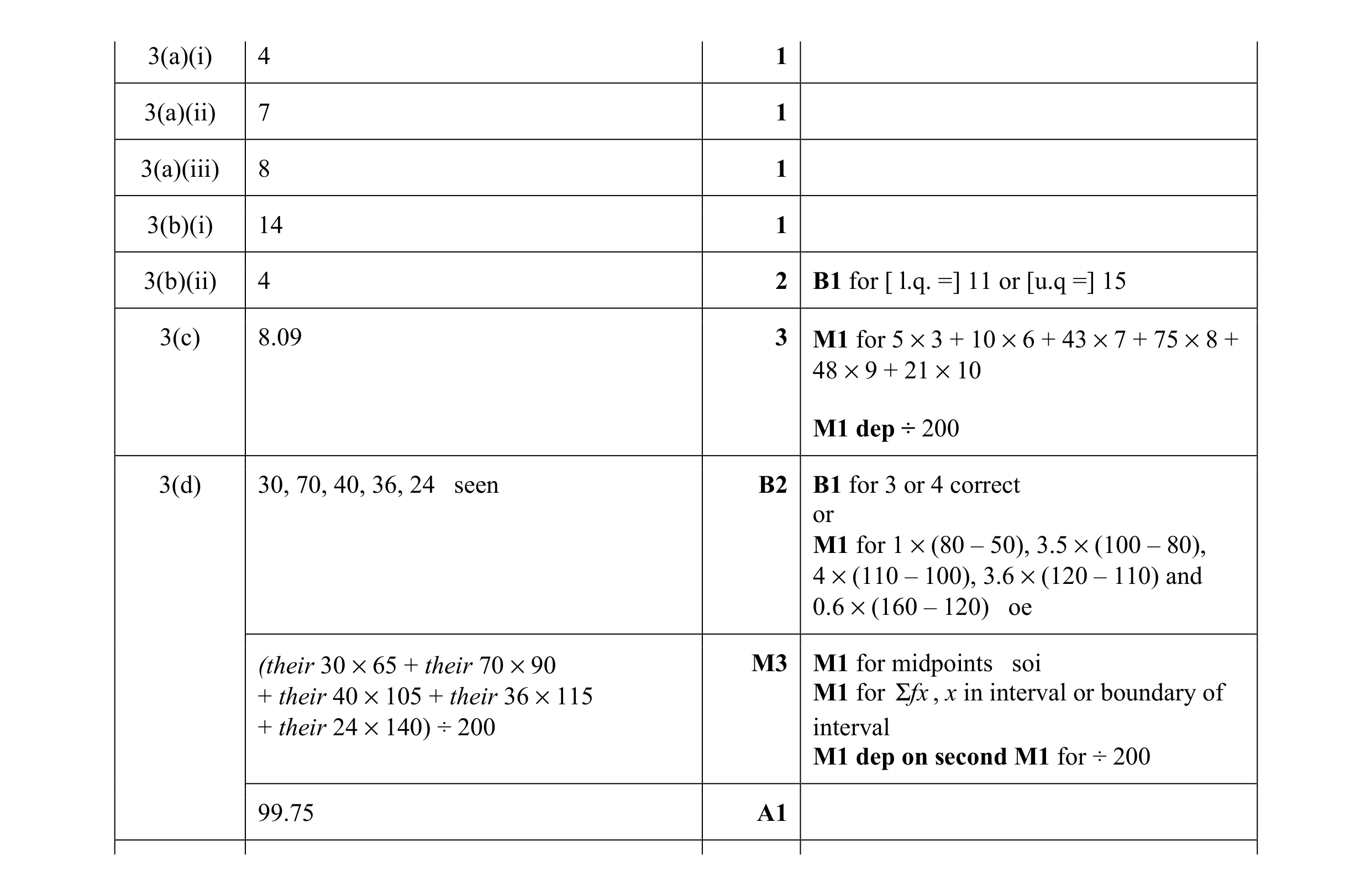 15
15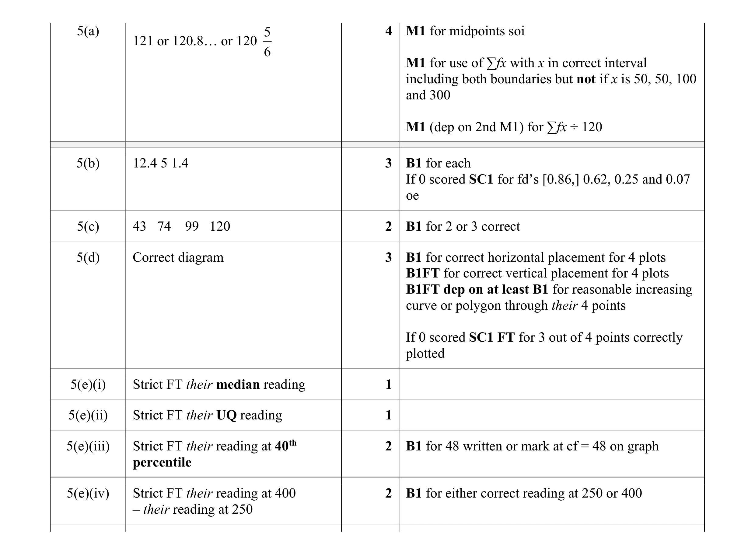 18
18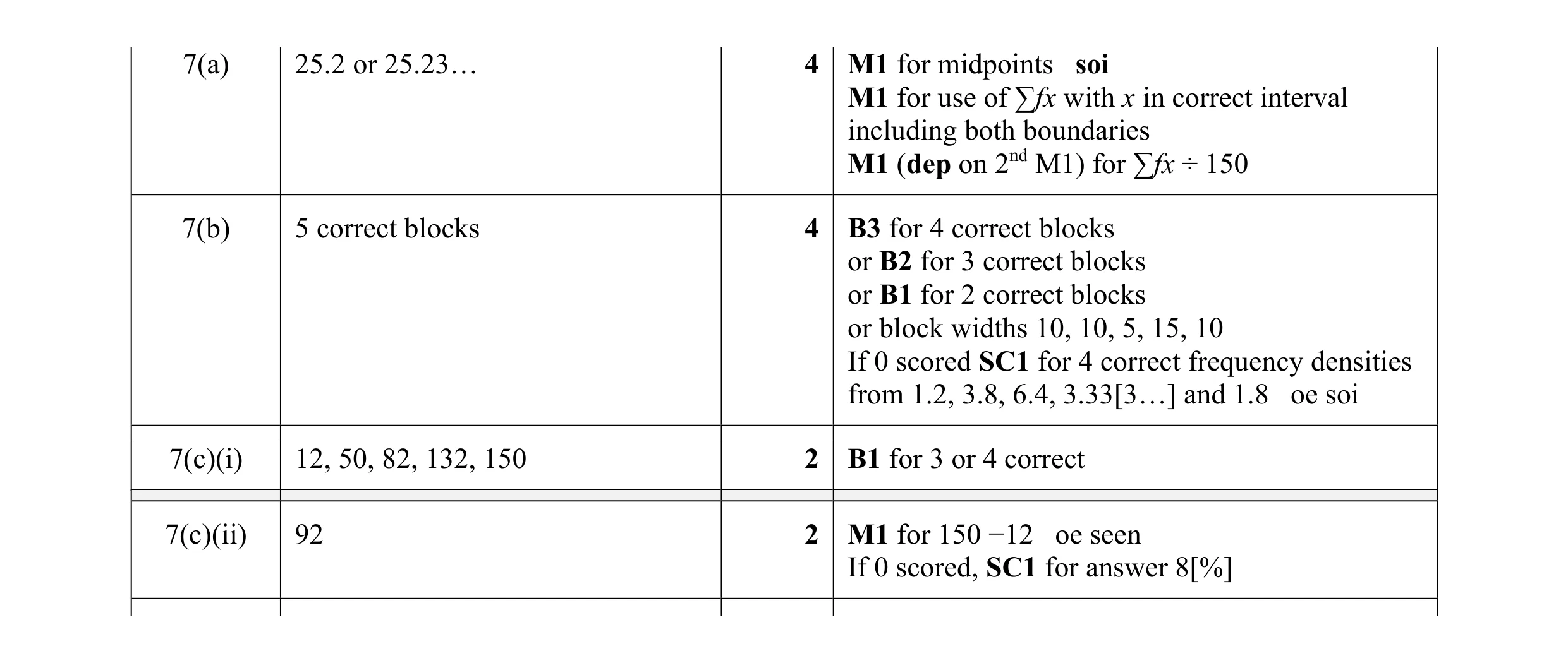 12
12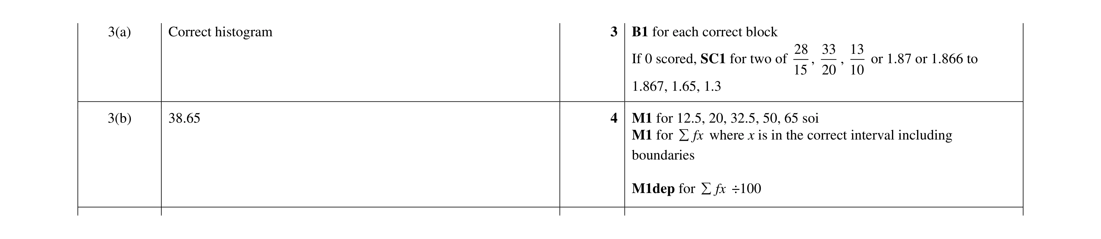 7
7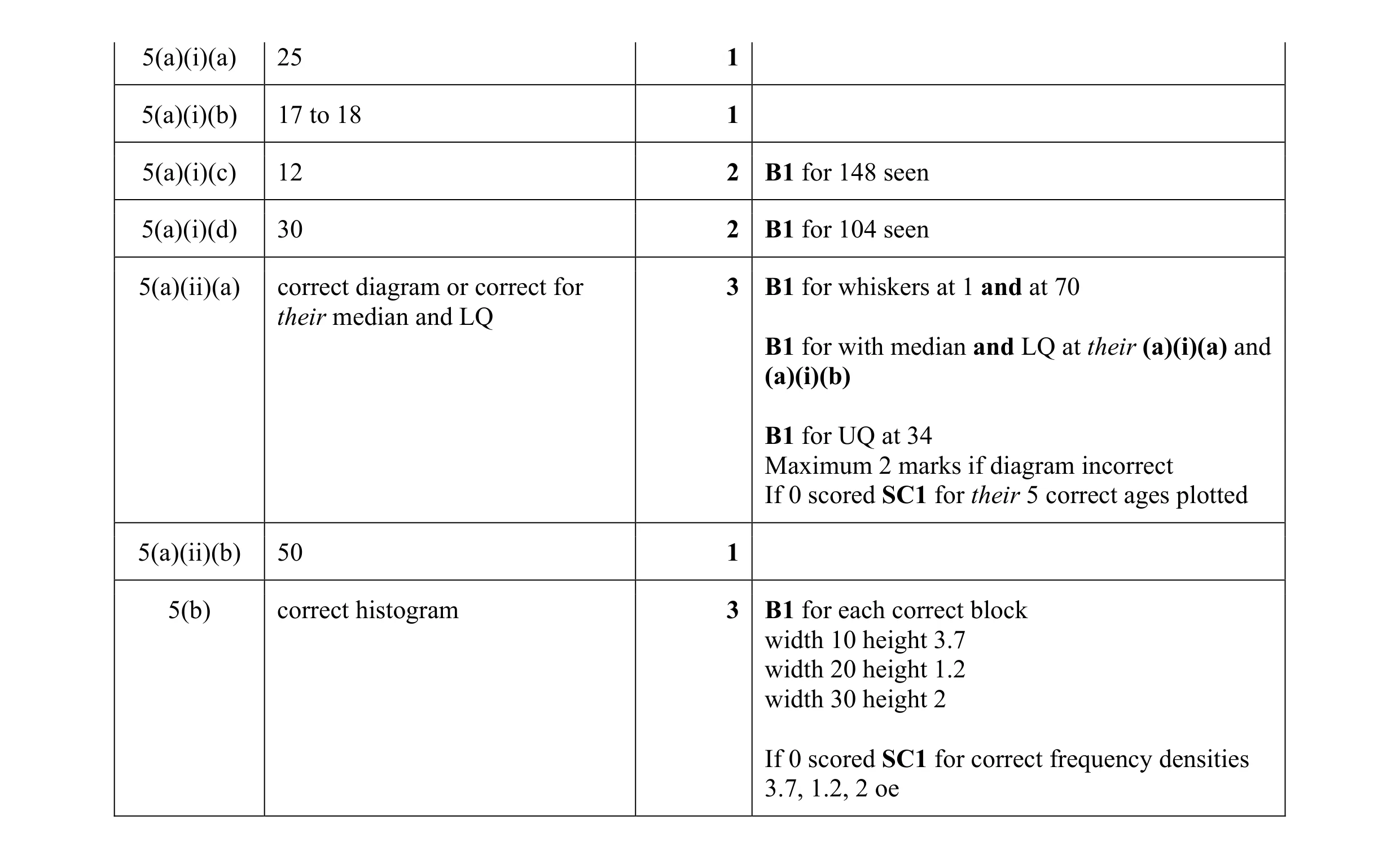 13
13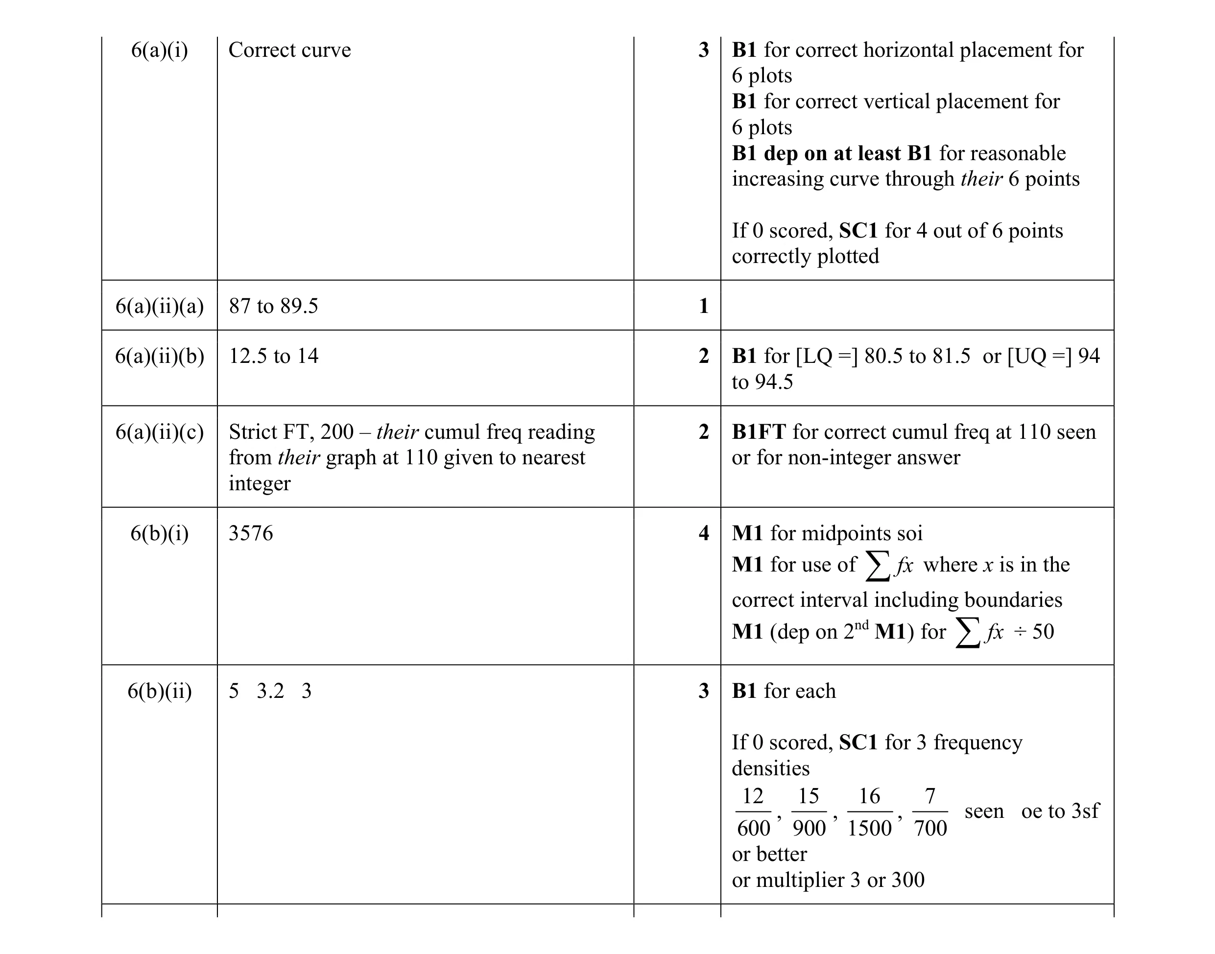 15
15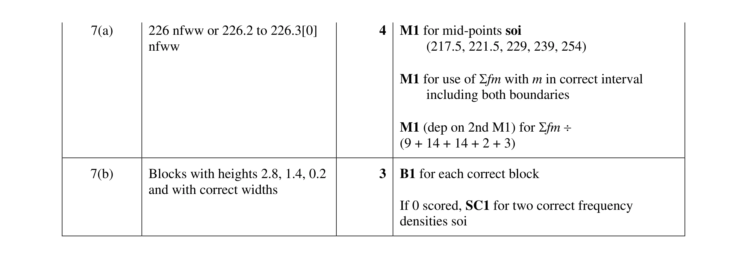 7
7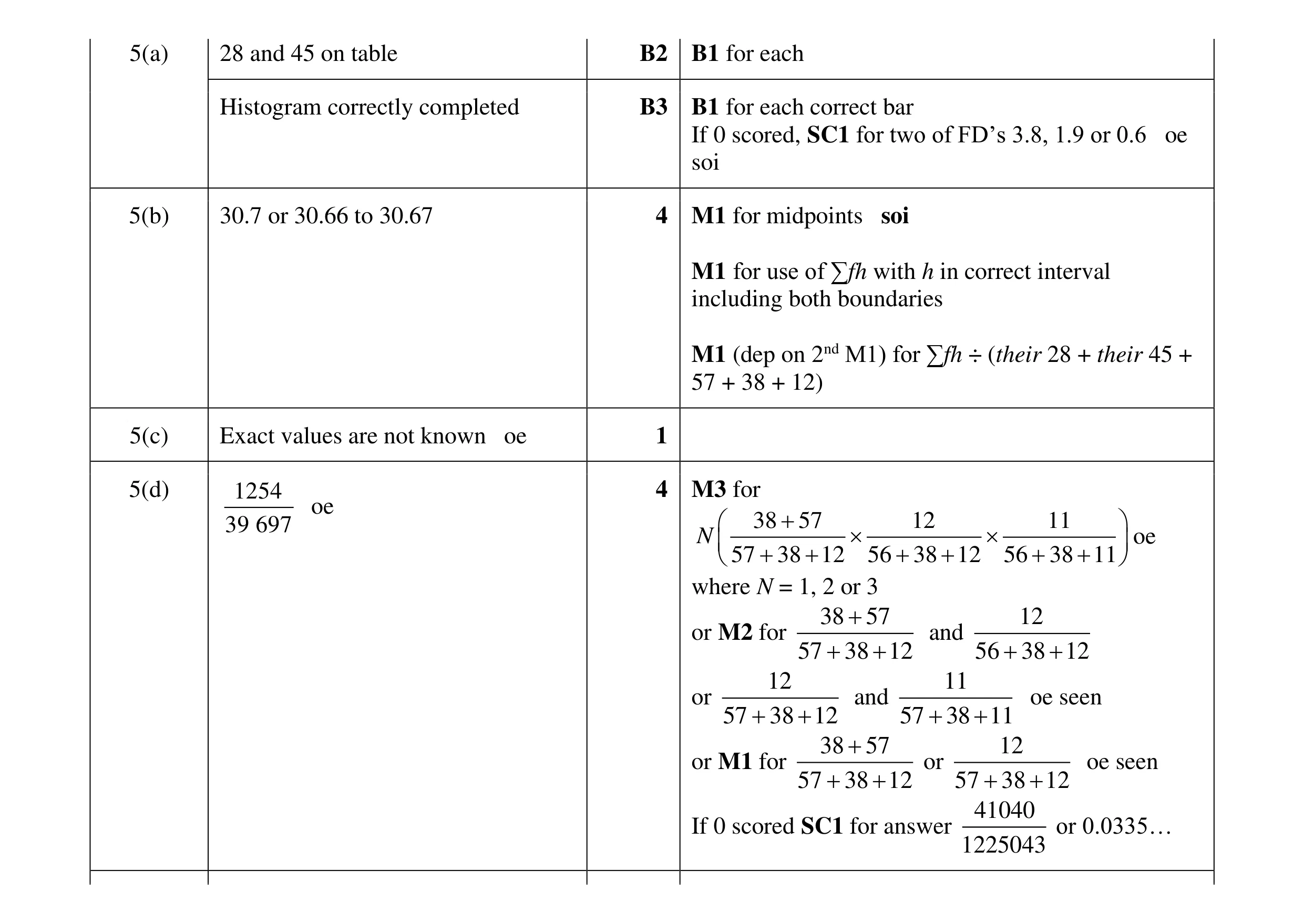 14
14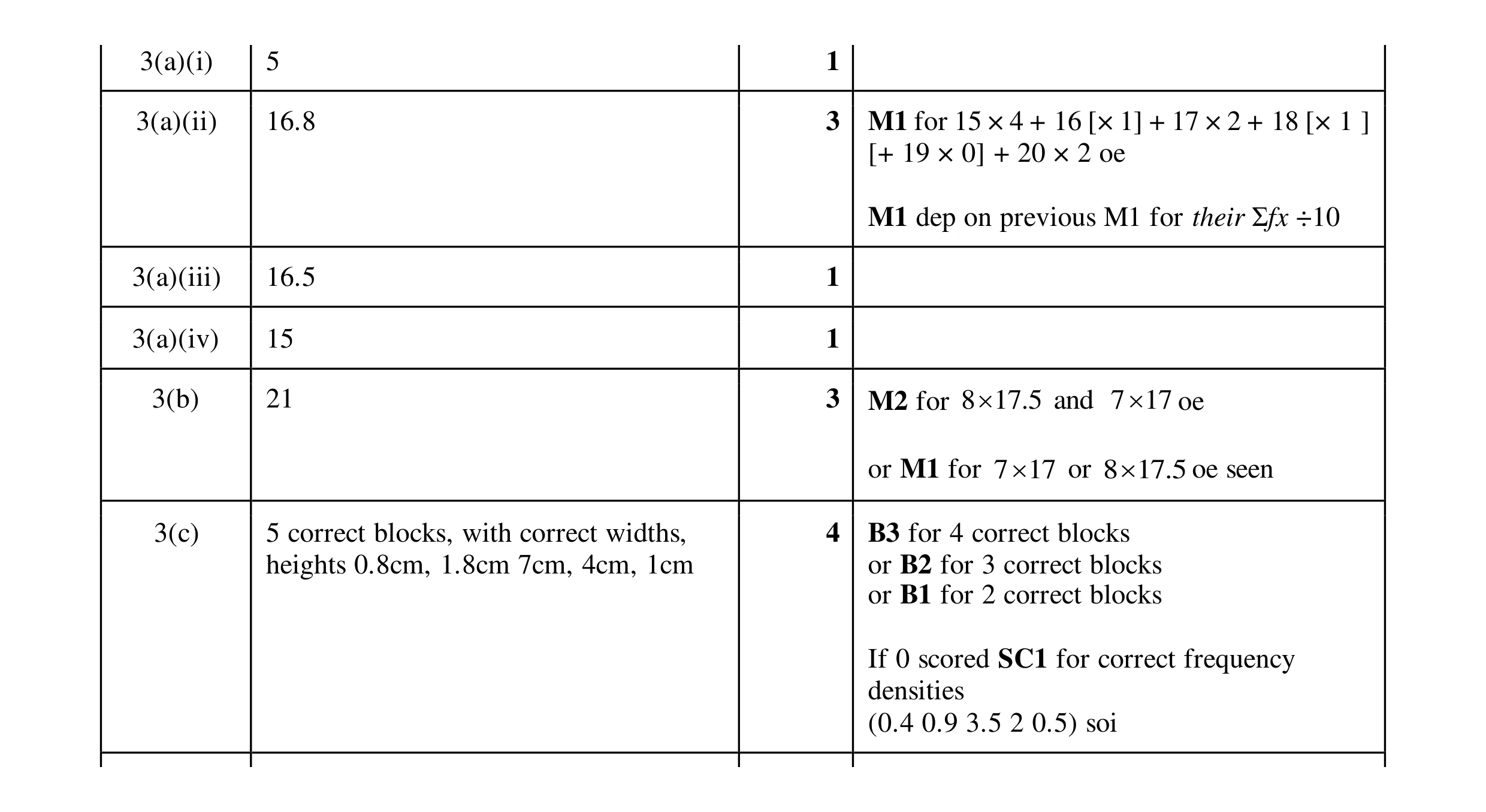 13
13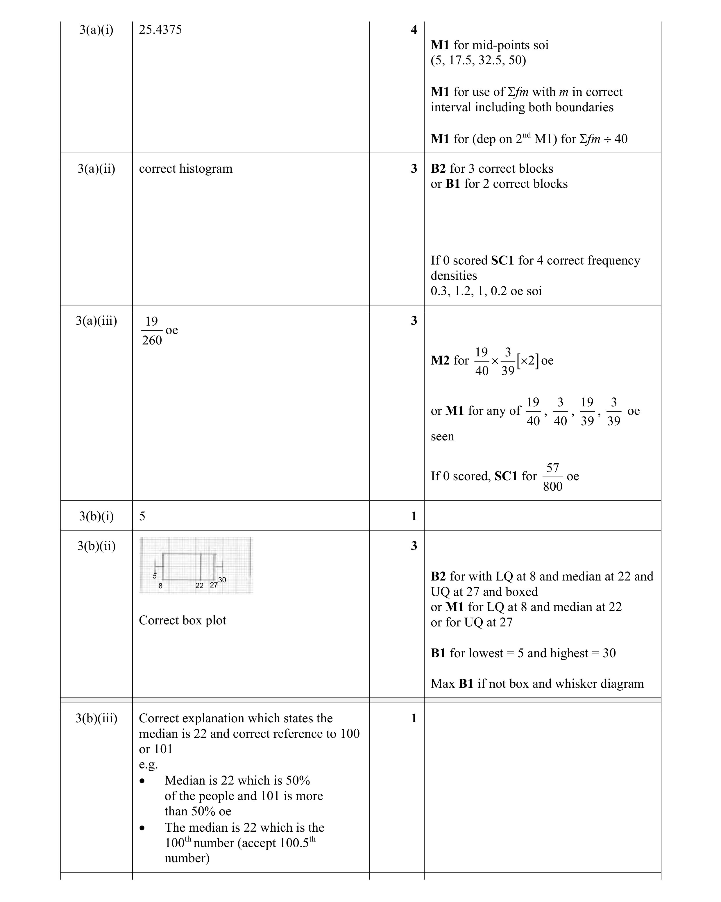 15
15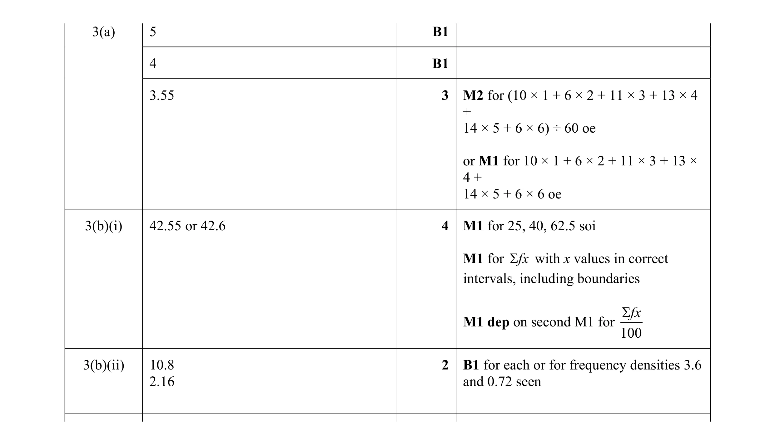 11
11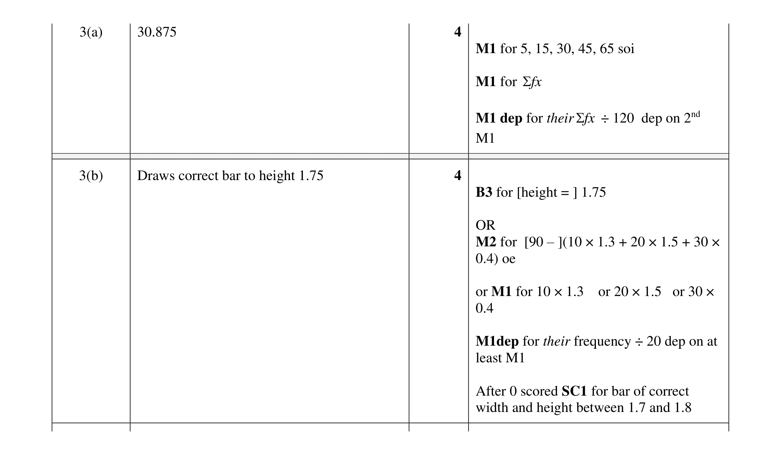 8
8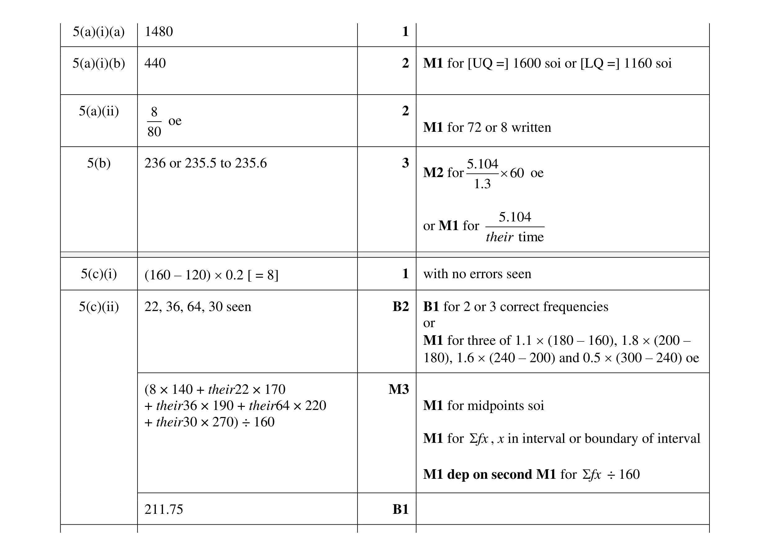 15
15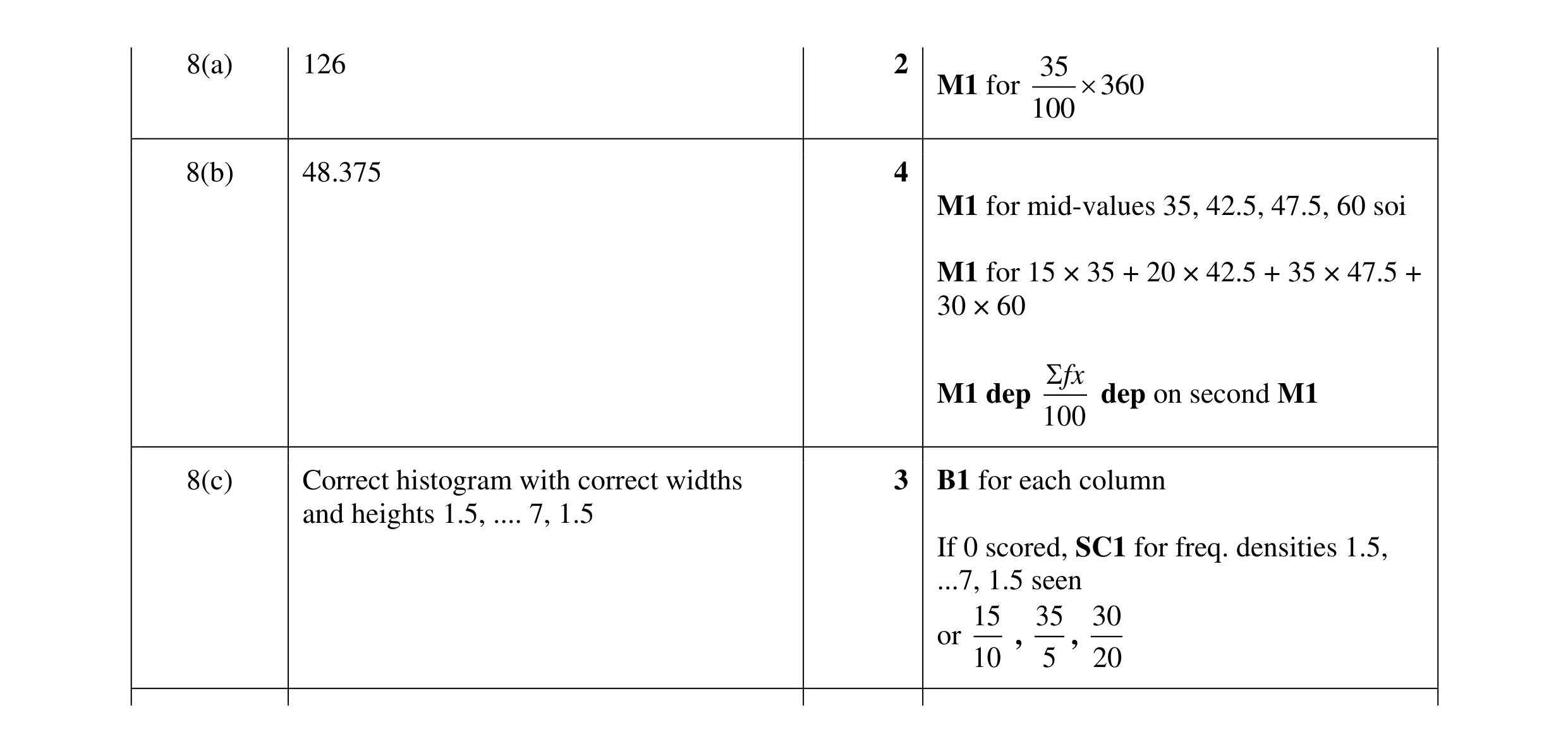 9
9 3
3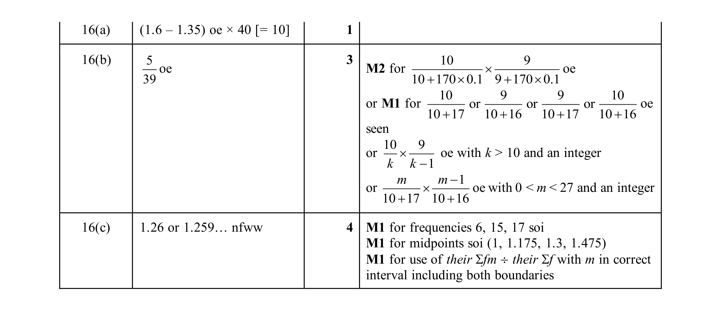 8
8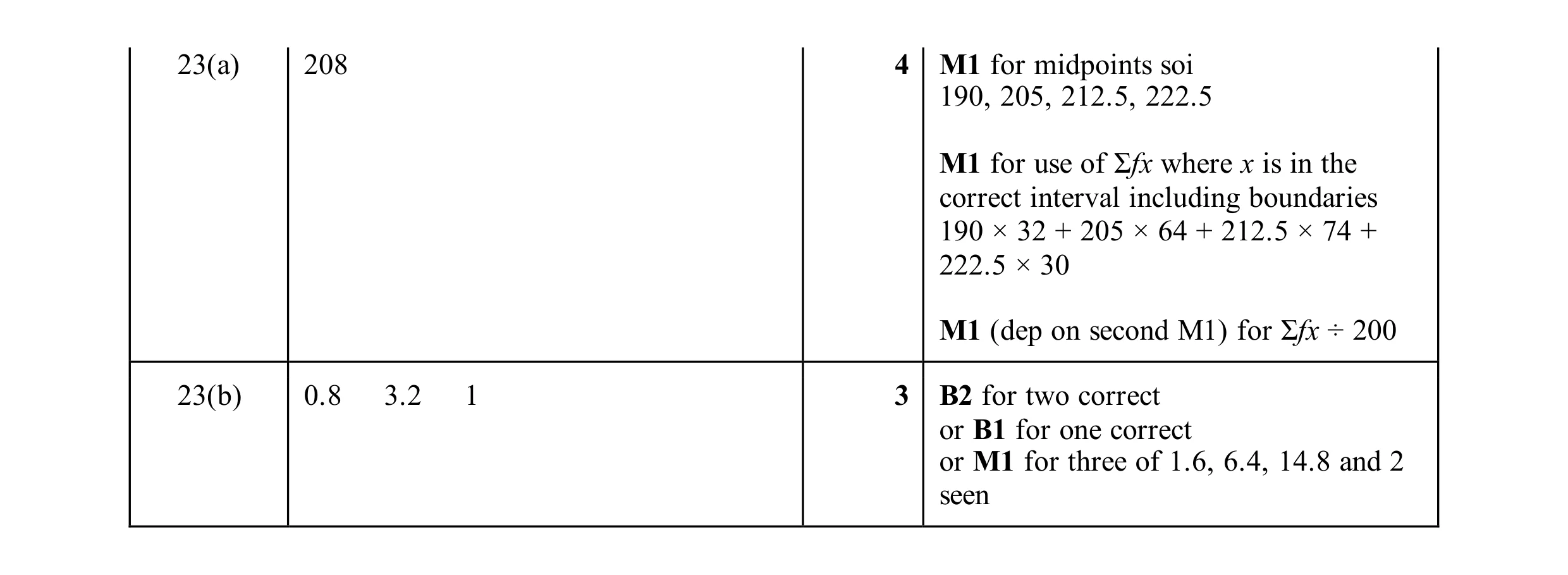 7
7