Questions as text
Q1 · Conducting putty is a soft material which can easily be made into different shapes 9702/51 May/June 2007
2 Conducting putty is a soft material which can easily be made into different shapes. It conducts electricity. An experiment was carried out to investigate how the resistance of a fixed volume of conducting putty varied with its length. The resistance of the conducting putty was measured using an ohmmeter, as shown in Fig. 2.1. ohmmeter metal metal contact contact cylinder of conducting putty plate plate l Fig. 2.1 Examiner’s Use Values of the length l of the conducting putty and the resistance R as measured by the ohmmeter are given in Fig. 2.2. l / cm R / Ω 6.0 ± 0.4 25 10.0 ± 0.4 60 14.0 ± 0.4 115 18.0 ± 0.4 185 22.0 ± 0.4 275 26.0 ± 0.4 380 Fig. 2.2 It is suggested that the resistivity ρ of the conducting putty is given by the formula (R – R0)V ________ ρ = l2 where R0 is the resistance of the connecting wires and V is the volume of the conducting putty. (a) Explain why plotting a graph of R against l2 would enable you to confirm the relationship between R and l. … … … [1] (b) Calculate and record values of l2, in cm2, in the table. Include in the table the absolute errors in l2. [3] (c) (i) Plot a graph of R (y-axis) against l2 (x-axis). Include error bars for l2. [2] (ii) Draw a best-fit straight line and a worst acceptable straight line on your graph. Both lines should be clearly labelled. [2] (iii) Determine the gradient of the best-fit line. Include the error in your answer. gradient = … [2] Examiner’s Use 400 350 300 R/Ω 250 200 150 100 50 0 0 100 200 300 400 500 600 700 l2/cm2 Question 2 continues over the page.
10 marks
Mark scheme: 2 Analysis, conclusions and evaluation (15 marks) Approach to data analysis (1 mark) ρl 2 (a) R = + R 0 and a correct comment. V This mark is not scored for R being proportional to l 2. [1] Table of results (2 marks) (b) Column heading for l 2. Allow l 2 / cm2 and l 2 (cm2) (or equivalent units). [1] (b) Values of l 2. [1] 36, 100, 196, 324, 484, 676 3 significant figures needed (except 1st row). Allow 4sf. All correct for one mark. Graph (3 marks) (c) (i) Points plotted correctly. [1] All six required for this mark and must be Ğ half a small square. Indicate an error. Ecf from (b) (c) (ii) Line of best fit. [1] Must be within tolerances. Do not allow a line forced through the origin. (c) (iii) Worst acceptable straight line. [1] Must be within tolerances. Line should be clearly labelled. Allow broken line. Conclusion (4 marks) (c) (iii) gradient of best-fit line [1] Gradient should be in the range 0.550 to 0.560. If (b) and/or (c)(i) and/or (ii) are incorrect then the triangle used should be greater than half the length of the drawn line. Check the read offs and ratio to be correct. Work to half a small square. (d) Value of ρ Candidate’s gradient value = ρ/V. May be implicit from working. [1] ρ in range 10.3 -10.6 [1] (d) Unit of ρ. Must be consistent with previous answer e.g. Ω cm [1] GCE A/AS LEVEL – May/June 2007 9702 05 Treatment of errors (5 marks) (b) Errors in l 2 [1] ± 4.6 – 5.0 ± 7.8 – 8.2 ± 11.0 – 11.4 ± 14.2 - 14 or 15 ± 17 or 18 ± 20 or 21 (c) (i) error bars in l 2 plotted correctly [1] Must be within tolerances. For ecf check first and last point (c) (iii) error in gradient [1] Check method e.g. gradient of best-fit line – gradient of worst acceptable line (d) correct method for determining error in ρ (e.g. (worst gradient × volume) - ρ) [1] Value for error in ρ in the range ± 0.4 to ± 0.6. [1] Last mark is zero if vertical error bars plotted or wrong worst acceptable line plotted. [Total: 15]
This question in 9702/51 May/June 2007
Q2 · A student wishes to measure the resistivity of glass 9702/51 May/June 2008
1 A student wishes to measure the resistivity of glass. A teacher suggests that its resistivity is For of the order of 106 Ω m which is very large. Examiner’s Use Resistivity ρ is defined by the equation RA ρ = l where R is resistance, A is cross-sectional area and l is the length of the material. The student is given a number of sheets of glass of the same thickness and of different areas. Design a laboratory experiment to determine the resistivity of glass. You should draw a diagram showing the arrangement of your equipment. In your account you should pay particular attention to (a) the procedure to be followed, (b) how the glass would be connected to the circuit, (c) the measurements that would be taken, (d) the control of variables, (e) how the data would be analysed, (f) any safety precautions that you would take. [15] Diagram For Examiner’s Use … … … … … … … … … … … … … … … For … Examiner’s Use … … … … … … … … … … … … … … … … … … … … … … … … … … …
15 marks
Mark scheme: 1 Planning (15 marks) Defining the problem (3 marks) P1 A is the independent variable or vary A. [1] P2 R is the dependent variable or determine R for different A. [1] P3 Keep the temperature (of glass) constant. Do not allow “controlled variable”. [1] Methods of data collection (5 marks) M1 Basic circuit diagram. [1] Ammeter and voltmeter with power supply, or ohmmeter without power supply, or bridge methods. M2 Correct orientation of glass between electrodes – largest cross-sectional area. [1] M3 A distance (thickness) measured using a micrometer/vernier scale/vernier callipers. [1] M4 Method of determining area perpendicular to current flow. [1] Distances measured and multiplied together. This mark may only be scored if it is clear that the correct dimensions are being used. M5 Method of determining resistance. [1] Ohmmeter. R = V/I justified. Description of balancing bridge with correct equation. Method of analysis (2 marks) A1 A2 R against 1/A ρ = gradient/l R against l /A ρ = gradient 1/A against R or 1/R against A ρ = 1/(gradient × l) l /A against R or l /R against A ρ = 1/gradient lg R against lg A ρ = 10l × y-intercept [2] Safety considerations (1 mark) S1 Relevant safety precaution related to: [1] EHT power supply (>100 V) – switch off before changing circuit/use of rubber gloves; or handling glass – wear (thick) gloves. Additional detail (4 marks) D1/2/3/4 Relevant points might include [4] Calculation of typical resistance of glass using value of resistivity given. Range of ammeter or ohmmeter with reasoning. Use of EHT or power supply >1000 V or microammeter/galvanometer. Take many readings of thickness and average. Good contact between circuit and glass e.g. metal plates, foil, conducting putty. Metal plates/foil/conducting putty to cover all of the cross-sectional area in use. Method of securing good contact between circuit and glass, e.g. g clamps, weights. Clean/dry the glass. [Total: 15] GCE A/AS LEVEL – May/June 2008 9702 05
This question in 9702/51 May/June 2008
Q3 · A hammer is often used to force a nail into wood 9702/51 May/June 2010
1 A hammer is often used to force a nail into wood. The faster the hammer moves, the deeper For the nail moves into the wood. Examiner’s Use This can be represented in a laboratory by a mass falling vertically onto a nail. It is suggested that the depth d of the nail in the wood (see Fig. 1.1) is related to the velocity v of the mass at the instant it hits the nail by the equation d = kv n where k and n are constants. nail d wood Fig. 1.1 Design a laboratory experiment to investigate the relationship between v and d so as to determine a value for n. You should draw a diagram showing the arrangement of your equipment. In your account you should pay particular attention to (a) the procedure to be followed, (b) the measurements to be taken, (c) the control of variables, (d) the analysis of the data, (e) the safety precautions to be taken. [15] Diagram For Examiner’s Use … … … … … … … … … … … … … … For … Examiner’s Use … … … … … … … … … … … … … … … … … … … … … … … Defining the Methods of Method of Safety Additional For problem data collection analysis considerations detail Examiner’s Use
15 marks
Mark scheme: 1 Planning (15 marks) Defining the problem (3 marks) P1 Vary v and measure d, or v is the independent variable and d is the dependent variable [1] P2 Keep mass constant [1] P3 Keep the wood constant/keep same type of nails [1] Methods of data collection (5 marks) M1 Diagram of apparatus showing mass falling onto centre of nail [1] M2 Change height of falling mass (to change v) [1] M3 Measurement(s) from which v can be determined, e.g. measure height fallen; light gate(s) connected to timer/data-logger measuring time, and ticker tape/motion sensor. Do not award stopwatch methods. [1] M4 Appropriate equation to determine v (the velocity of the mass at the instant it hits the nail) [1] M5 Detail on measuring d ; subtract, needle, mark nail, depth gauge [1] Method of analysis (2 marks) A1 Plot a graph of log d against log v [1] A2 n = gradient [1] Safety considerations (1 mark) S1 Precaution linked to falling masses, e.g. keep well away/sand trays [1] Additional detail (4 marks) D 1/2/3/4 Relevant points might include [4] 1. Method to create a large d, e.g. large mass, thin nails, soft wood 2. Use of a guide for falling mass/guide for nail 3. Use of vernier scale to measure d 4. Repeat experiment and determine an average 5. Use different part of wood for each test 6. Method to make nail vertical e.g. set square 7. Discussion / preliminary experiment about thin nails going totally into wood 8. lg d = n lg v + lg k [Total: 15] GCE AS/A LEVEL – May/June 2010 9702 51
This question in 9702/51 May/June 2010
Q4 · A student is investigating how the period T of a simple pendulum depends on its For… 9702/51 Oct/Nov 2010
2 A student is investigating how the period T of a simple pendulum depends on its For length l , as shown in Fig. 2.1. Examiner’s Use l Fig. 2.1 The time t for 10 oscillations is recorded for a pendulum of length l. The period T of the pendulum is determined. The procedure is then repeated for different lengths. Question 2 continues on the next page. It is suggested that T and l are related by the equation For Examiner’s T = al b Use where a and b are constants. (a) A graph is plotted of lg T on the y-axis and lg l on the x-axis. Determine expressions for the gradient and y-intercept in terms of a and b. gradient = … y-intercept = … [1] (b) Values of l and t are given in Fig. 2.2. l / cm t / s T / s lg (l / cm) lg (T / s) 95.0 19.6 ± 0.2 85.0 18.4 ± 0.2 75.0 17.4 ± 0.2 65.0 16.2 ± 0.2 55.0 14.8 ± 0.2 45.0 13.4 ± 0.2 Fig. 2.2 Calculate and record values of T / s, lg (l / cm) and lg (T / s) in Fig. 2.2. Include the absolute uncertainties in lg (T / s). [3] (c) (i) Plot a graph of lg (T / s) against lg (l / cm). Include error bars for lg (T / s). [2] (ii) Draw the straight line of best fit and a worst acceptable straight line on your graph. Both lines should be clearly labelled. [2] (iii) Determine the gradient of the line of best fit. Include the uncertainty in your answer. gradient = … [2] For 0.32 Examiner’s Use 0.30 0.28 lg (T / s) 0.26 0.24 0.22 0.20 0.18 0.16 0.14 0.12 0.10 1.65 1.70 1.75 1.80 1.85 1.90 1.95 2.00 lg (l / cm)
10 marks
Mark scheme: 2 Analysis, conclusions and evaluation (15 marks) Part Mark Expected Answer Additional Guidance (a) A1 Gradient = b Allow log a but not ln a y-intercept = lg a (b) T1 T1 for lg l column – ignore rounding errors; min T2 1.9777 0.292 or 0.2923 2 dp. 1.9294 0.265 or 0.2648 T2 for lg T column – must be values given A mixture is allowed 1.8751 0.241 or 0.2405 1.8129 0.210 or 0.2095 1.7404 0.170 or 0.1703 1.6532 0.127 or 0.1271 U1 From ± 0.004 or ± 0.005 to ± 0.006 Allow more than one significant figure. or ± 0.007 (c) (i) G1 Six points plotted correctly Must be within half a small square; penalise ≥ half a small square. Penalise ‘blobs’ ≥ half a small square. Ecf allowed from table. U2 Error bars in lg (T/s) plotted All error bars must be plotted. Check first and correctly. last point. Must be accurate within half a small square; penalise ≥ half a small square. (ii) G2 Line of best fit If points are plotted correctly then lower end of line should pass between (1.65, 0.124) and (1.65, 0.128) and upper end of line should pass between (2.00, 0.300) and (2.00, 0.306). Allow ecf from points plotted incorrectly; five trend plots needed – examiner judgement. G3 Worst acceptable straight line. Line should be clearly labelled or dashed. Steepest or shallowest possible Should pass from top of top error bar to bottom line that passes through all the of bottom error bar or bottom of top error bar to error bars. top of bottom error bar. Mark scored only if all error bars are plotted. (iii) C1 Gradient of best fit line The triangle used should be at least half the length of the drawn line. Check the read offs. Work to half a small square; penalise ≥ half a small square. U3 Uncertainty in gradient Method of determining absolute uncertainty Difference in worst gradient and gradient. (iv) C2 y-intercept Must be negative. Check substitution of point from line into c = y – mx. Allow ecf from (c)(iii). GCE A/AS LEVEL – October/November 2010 9702 51 U4 Uncertainty in y-intercept Method of determining absolute uncertainty Difference in worst y-intercept and y-intercept. Do not allow ecf from false origin read-off (FOX). Allow ecf from (c)(iv). (d) C3 a = 10y-intercept y-intercept must be used. Expect an answer of about 0.19. If FOX expect answer of about 1.3. C4 b = gradient and in the range 0.495 Allow 0.50 to 0.52 to 2 sf to 0.520 and to 2 or 3 sf Penalise 1 sf or ≥4 sf U5 Absolute uncertainty in a and b Difference in a and worst a. Uncertainty in b should be the same as the uncertainty in the gradient. [Total: 15] Uncertainties in Question 2 (c) (iii) Gradient [U3] 1. Uncertainty = gradient of line of best fit – gradient of worst acceptable line 2. Uncertainty = ½ (steepest worst line gradient – shallowest worst line gradient) (c) (iv) [U4] 1. Uncertainty = y-intercept of line of best fit – y-intercept of worst acceptable line 2. Uncertainty = ½ (y-intercept of steepest worst line – y-intercept of shallowest worst line) (d) [U5] 1. Uncertainty = 10 best y-intercept - 10 worst y-intercept
This question in 9702/51 Oct/Nov 2010
Q5 · A student is investigating how the period T of a simple pendulum depends on its For… 9702/52 Oct/Nov 2010
2 A student is investigating how the period T of a simple pendulum depends on its For length l , as shown in Fig. 2.1. Examiner’s Use l Fig. 2.1 The time t for 10 oscillations is recorded for a pendulum of length l. The period T of the pendulum is determined. The procedure is then repeated for different lengths. Question 2 continues on the next page. It is suggested that T and l are related by the equation For Examiner’s T = al b Use where a and b are constants. (a) A graph is plotted of lg T on the y-axis and lg l on the x-axis. Determine expressions for the gradient and y-intercept in terms of a and b. gradient = … y-intercept = … [1] (b) Values of l and t are given in Fig. 2.2. l / cm t / s T / s lg (l / cm) lg (T / s) 95.0 19.6 ± 0.2 85.0 18.4 ± 0.2 75.0 17.4 ± 0.2 65.0 16.2 ± 0.2 55.0 14.8 ± 0.2 45.0 13.4 ± 0.2 Fig. 2.2 Calculate and record values of T / s, lg (l / cm) and lg (T / s) in Fig. 2.2. Include the absolute uncertainties in lg (T / s). [3] (c) (i) Plot a graph of lg (T / s) against lg (l / cm). Include error bars for lg (T / s). [2] (ii) Draw the straight line of best fit and a worst acceptable straight line on your graph. Both lines should be clearly labelled. [2] (iii) Determine the gradient of the line of best fit. Include the uncertainty in your answer. gradient = … [2] For 0.32 Examiner’s Use 0.30 0.28 lg (T / s) 0.26 0.24 0.22 0.20 0.18 0.16 0.14 0.12 0.10 1.65 1.70 1.75 1.80 1.85 1.90 1.95 2.00 lg (l / cm)
10 marks
Mark scheme: 2 Analysis, conclusions and evaluation (15 marks) Part Mark Expected Answer Additional Guidance (a) A1 Gradient = b Allow log a but not ln a y-intercept = lg a (b) T1 T1 for lg l column – ignore rounding errors; min T2 1.9777 0.292 or 0.2923 2 dp. 1.9294 0.265 or 0.2648 T2 for lg T column – must be values given A mixture is allowed 1.8751 0.241 or 0.2405 1.8129 0.210 or 0.2095 1.7404 0.170 or 0.1703 1.6532 0.127 or 0.1271 U1 From ± 0.004 or ± 0.005 to ± 0.006 Allow more than one significant figure. or ± 0.007 (c) (i) G1 Six points plotted correctly Must be within half a small square; penalise ≥ half a small square. Penalise ‘blobs’ ≥ half a small square. Ecf allowed from table. U2 Error bars in lg (T/s) plotted All error bars must be plotted. Check first and correctly. last point. Must be accurate within half a small square; penalise ≥ half a small square. (ii) G2 Line of best fit If points are plotted correctly then lower end of line should pass between (1.65, 0.124) and (1.65, 0.128) and upper end of line should pass between (2.00, 0.300) and (2.00, 0.306). Allow ecf from points plotted incorrectly; five trend plots needed – examiner judgement. G3 Worst acceptable straight line. Line should be clearly labelled or dashed. Steepest or shallowest possible Should pass from top of top error bar to bottom line that passes through all the of bottom error bar or bottom of top error bar to error bars. top of bottom error bar. Mark scored only if all error bars are plotted. (iii) C1 Gradient of best fit line The triangle used should be at least half the length of the drawn line. Check the read offs. Work to half a small square; penalise ≥ half a small square. U3 Uncertainty in gradient Method of determining absolute uncertainty Difference in worst gradient and gradient. (iv) C2 y-intercept Must be negative. Check substitution of point from line into c = y – mx. Allow ecf from (c)(iii). GCE A/AS LEVEL – October/November 2010 9702 52 U4 Uncertainty in y-intercept Method of determining absolute uncertainty Difference in worst y-intercept and y-intercept. Do not allow ecf from false origin read-off (FOX). Allow ecf from (c)(iv). (d) C3 a = 10y-intercept y-intercept must be used. Expect an answer of about 0.19. If FOX expect answer of about 1.3. C4 b = gradient and in the range 0.495 Allow 0.50 to 0.52 to 2 sf to 0.520 and to 2 or 3 sf Penalise 1 sf or ≥4 sf U5 Absolute uncertainty in a and b Difference in a and worst a. Uncertainty in b should be the same as the uncertainty in the gradient. [Total: 15] Uncertainties in Question 2 (c) (iii) Gradient [U3] 1. Uncertainty = gradient of line of best fit – gradient of worst acceptable line 2. Uncertainty = ½ (steepest worst line gradient – shallowest worst line gradient) (c) (iv) [U4] 1. Uncertainty = y-intercept of line of best fit – y-intercept of worst acceptable line 2. Uncertainty = ½ (y-intercept of steepest worst line – y-intercept of shallowest worst line) (d) [U5] 1. Uncertainty = 10 best y-intercept - 10 worst y-intercept
This question in 9702/52 Oct/Nov 2010
Q6 · A student wishes to determine the resistivity of aluminium 9702/53 Oct/Nov 2010
1 A student wishes to determine the resistivity of aluminium. For Examiner’s The resistivity ρ of a conductor is defined as Use RA ρ = l for a conductor of resistance R, cross-sectional area A and length l. Fig. 1.1 shows the typical dimensions of a strip of aluminium of lengths c, d and t. The resistivity of aluminium is about 10–8 Ωm. t = 1 mm d 1 cm c 1 m Fig. 1.1 (not to scale) Design a laboratory experiment to determine the resistivity of aluminium using this strip. The usual apparatus of a school laboratory is available, including a metal cutter. You should draw a diagram, on page 3, showing the arrangement of your equipment. In your account you should pay particular attention to (a) the procedure to be followed, (b) the measurements to be taken, (c) the control of variables, (d) the analysis of the data, (e) the safety precautions to be taken. [15] Diagram For Examiner’s Use … … … … … … … … … … … … … … For … Examiner’s Use … … … … … … … … … … … … … … … … … … … … … … … Defining the Methods of Method of Safety Additional For problem data collection analysis considerations detail Examiner’s Use
15 marks
Mark scheme: 1 Planning (15 marks) Defining the problem (3 marks) P1 c, d or A is the independent variable and R is the dependent variable or vary c, d or A and measure R. [1] P2 If c varied then (t and) d or A kept constant, if d varied then (t and) c or A kept constant, if A varied then c or d kept constant. [1] P3 Keep temperature constant. [1] Methods of data collection (5 marks) M1 Circuit diagram to measure resistance. [1] M2 Use micrometer screw gauge to measure d or t. (Allow digital or vernier callipers) [1] M3 Measure c with a ruler/metre rule. [1] M4 Method of making contact with the strip e.g. use electrodes of at least same dimension as c or d or t or conducting paint methods. Do not allow crocodile clips, unless it is clear that the whole area of the end of the strip is covered. [1] M5 Method to determine resistance. [1] Method of analysis (2 marks) A1 Plot a graph of R against c, 1/d or 1/A depending on orientation. Other alternatives possible, e.g. R against 1/c depending on orientation [1] A2 Must be consistent with A1: ρ = A × gradient or t × gradient/c [1] Other alternatives possible, e.g. ρ = d × gradient/t Safety considerations (1 mark) S1 Reference sharp edges or cutting metals, e.g. wear gloves. [1] Additional detail (4 marks) D1/2/3/4 Relevant points might include [4] 1. Insulate aluminium strip 2. Take many readings of t or d and average 3. Use a protective resistor/circuit designed to reduce current 4. Rearrange equation to determine graph using c, d and t or A 5. Determine typical resistance of aluminium strip 6. Likely meter range of ammeter/voltmeter/ohmmeter 7. Detail on cutting strip e.g. mark using set square Do not allow vague computer methods. [Total: 15] GCE A/AS LEVEL – October/November 2010 9702 53
This question in 9702/53 Oct/Nov 2010
Q7 · A student is investigating how a volume of nitrogen gas is affected by the pressure… 9702/51 May/June 2011
2 A student is investigating how a volume of nitrogen gas is affected by the pressure exerted For on it. Examiner’s Use A sample of nitrogen gas is trapped in a vertical tube of uniform cross-sectional area by a small volume of oil. Pressure is applied by a pump. The applied pressure is measured on a gauge, as shown in Fig. 2.1. nitrogen h pressure gauge oil pump air Fig. 2.1 The temperature T of the nitrogen is 290 K. An experiment is carried out to investigate how the height h of nitrogen trapped in the tube varies with the pressure p. Question 2 continues on the next page. It is suggested that p and h are related by the equation For Examiner’s pAh = NkT Use where A is the cross-sectional area of the tube, k is the Boltzmann constant and N is the number of molecules of nitrogen gas. 1 (a) A graph is plotted of p on the y-axis against on the x-axis. Express the gradient in h terms of N. gradient = … [1] (b) Values of p and h are given in Fig. 2.2. p / 105 Pa h / 10–3 m 1.10 400 ± 5 1.22 360 ± 5 1.38 320 ± 5 1.57 280 ± 5 1.83 240 ± 5 2.09 210 ± 5 Fig. 2.2 1 1 Calculate and record values of in Fig. 2.2. Include the absolute uncertainties in . h h [3] 1 1(c) (i) Plot a graph of p / 105 Pa against / m–1. Include error bars for [2] h h. (ii) Draw the straight line of best fit and a worst acceptable straight line on your graph. Both lines should be clearly labelled. [2] (iii) Determine the gradient of the line of best fit. Include the uncertainty in your answer. gradient = … [2] 2.1 For Examiner’s Use 2.0 1.9 p / 105 Pa 1.8 1.7 1.6 1.5 1.4 1.3 1.2 1.1 1.0 2.0 2.5 3.0 3.5 4.0 4.5 5.0 5.5 1 / m–1 h
10 marks
Mark scheme: 2 Analysis, conclusions and evaluation (15 marks) Part Mark Expected Answer Additional Guidance (a) A1 NkT/A 290Nk/A (b) T1 1 Column heading. Allow equivalent unit. / m–1 h e.g. h–1 / m–1 T2 2.5 or 2.50 A mixture of 2sf and 3sf is allowed. 2.8 or 2.78 3.1 or 3.13 3.6 or 3.57 4.2 or 4.17 4.8 or 4.76 U1 From ± 0.03 to ± 0.1, ± 0.11 or ± 0.12 Allow more than one significant figure. (c) (i) G1 Six points plotted correctly Check second and fifth plots and other anomalous plots. Must be less than half a small square. Ecf allowed from table. U2 1 Half square or greater loses the mark. Ecf All error bars in plotted correctly h allowed from table. (ii) G2 Line of best fit If points are plotted correctly then lower end of line should pass between (2.20, 1.0) and (2.30, 1.0) and upper end of line should pass between (4.75, 2.1) and (4.85, 2.1). Allow ecf from points plotted incorrectly – examiner judgement. G3 Worst acceptable straight line. Line should be clearly labelled or dashed. Steepest or shallowest possible line Should pass from top of top error bar to that passes through all the error bars. bottom of bottom error bar or bottom of top error bar to top of bottom error bar. Mark scored only if error bars are plotted. (iii) C1 Gradient of best fit line The triangle used should be at least half the length of the drawn line. Check the read offs. Work to half a small square. Do not penalise POT. U3 Uncertainty in gradient Method of determining absolute uncertainty Difference in worst gradient and gradient. (d) C2 gradient × A Gradient must be used. Value of N = Allow ecf from (c)(iii) but penalise POT. kT U4 Determines uncertainty in N Method required. Do not check calculation. (e) (i) C3 Method to determine h NkT −20 h = = 1.111 × 10 × N ; T = 278 K pA Must use answer from (d). C4 Between 0.361 and 0.391 given to 2 or Must be in range. Allow 0.36, 0.37, 0.38 or 3 sf 0.39. Assume metres unless otherwise specified. (ii) U5 Percentage uncertainty % uncertainty in N + % uncertainty in T) [Allow ∆T to be 0.5 or 1] [Total: 15] GCE AS/A LEVEL – May/June 2011 9702 51 Uncertainties in Question 2 (c) (iii) Gradient [U3] Uncertainty = gradient of line of best fit – gradient of worst acceptable line Uncertainty = ½ (steepest worst line gradient – shallowest worst line gradient) (d) [U4] Uncertainty = worst N – N ∆m ∆N = × N m A ∆N = ∆m × kT (e) [U5] ∆h Percentage uncertainty = × 100 h Percentage uncertainty = percentage uncertainty in N + percentage uncertainty in T
This question in 9702/51 May/June 2011
Q8 · A student wishes to investigate projectile motion 9702/52 May/June 2011
1 A student wishes to investigate projectile motion. For Examiner’s A small ball is rolled with velocity v along a horizontal surface. When the ball reaches the Use end of the horizontal surface, it falls and lands on a lower horizontal surface. The vertical displacement of the ball is p and the horizontal displacement of the ball is q, as shown in Fig 1.1. v p q Fig. 1.1 It is suggested that gq 2 = 2pv 2 where g is the acceleration of free fall. Design a laboratory experiment to investigate how q is related to p and how v may be determined from the results. You should draw a diagram, on page 3, showing the arrangement of your equipment. In your account you should pay particular attention to (a) the procedure to be followed, (b) the measurements to be taken, (c) the control of variables, (d) the analysis of the data, (e) the safety precautions to be taken. [15] Diagram For Examiner’s Use … … … … … … … … … … … … … … … For … Examiner’s Use … … … … … … … … … … … … … … … … … … … … … … … Defining the Methods of Method of Safety Additional For problem data collection analysis considerations detail Examiner’s Use
15 marks
Mark scheme: 1 Planning (15 marks) Defining the problem (3 marks) P1 p is the independent variable or vary p [1] P2 q is the dependent variable or measure q [1] P3 Keep (horizontal) velocity (v) constant [1] Methods of data collection (5 marks) M1 Labelled diagram of apparatus including method to vary p. [1] M2 Method to determine position of ball on surface e.g. carbon paper/dye/video/sand. [1] M3 Use ruler/caliper to measure p and/or q. [1] M4 Method to ensure velocity is constant e.g. releasing ball from same height on a track/ spring loaded device or impulse device set to a constant value. [1] M5 Method to ensure that the moved surface remains horizontal, e.g. spirit level/check height at different places. [1] Method of analysis (2 marks) A1 q2 against p q against p p against q2 p against q [1] g × gradient g g 1 g A2 v = v = gradient × v = v = × [1] 2 2 2× gradient gradient 2 Allow valid logarithmic graph e.g. lg q against lg p, lg 2p, lg 2p/g and valid calculation of v from y-intercept. Safety considerations (1 mark) S Reasoned method to prevent ball rolling on floor e.g. box below/storage box for balls/ sand box. Reasoned method to prevent ball causing injury e.g. goggles/safety screen [1] Additional detail (4 marks) D Relevant points might include [4] 1 Method to ensure that velocity of ball is horizontal only when it reaches table, e.g. curved track. 2 Ensure that the ball leaves the table at 90°, e.g. set square/protractor on upper surface. 3 Detail on measuring q – location of landing position e.g. centre of crater/start of track. 4 Detail on determining location of zero position for p and q e.g. set square, plumb line. 5 Detail on method of determining position of ball e.g. slow motion playback including scale. 6 Take many readings of q for each p and average. 7 Straight line through the origin shows that p is proportional to q2/relationship is valid – this mark may only be awarded when A1 is given. 8 Use of high density ball to minimise the effects of air resistance. Do not allow vague computer methods. [Total: 15] GCE AS/A LEVEL – May/June 2011 9702 52
This question in 9702/52 May/June 2011
Q9 · A student is investigating a non-inverting operational amplifier (op-amp) circuit 9702/52 May/June 2011
2 A student is investigating a non-inverting operational amplifier (op-amp) circuit. For Examiner’s The circuit is set up as shown in Fig. 2.1. Use +18 V + – E F –18 V V R Fig. 2.1 The op-amp is connected to a +18 V and –18 V power supply. E is the e.m.f. of the cell, which has a value of 1.6 ± 0.1 V. An experiment is carried out to investigate how the reading V on the voltmeter varies with resistance R. Question 2 continues on the next page. It is suggested that V and R are related by the equation For Examiner’s F Use V = E + E R where F is the resistance of the fixed resistor in the circuit. V 1(a) A graph is plotted of on the y-axis against on the x-axis. Express the gradient in E R terms of F. gradient = … [1] (b) Values of R and V are given in Fig. 2.2. R / Ω V / V 1 V / 10–3 Ω–1 R E 150 14.4 ± 0.1 220 10.4 ± 0.1 330 7.4 ± 0.1 470 5.6 ± 0.1 680 4.4 ± 0.1 860 3.8 ± 0.1 Fig. 2.2 1 V Calculate and record values of / 10–3 Ω–1 and in Fig. 2.2. Include the absolute R E V uncertainties in . [3] E V 1 V (c) (i) Plot a graph of against / 10–3 Ω–1. Include error bars for . [2] E R E (ii) Draw the straight line of best fit and a worst acceptable straight line on your graph. Both lines should be clearly labelled. [2] (iii) Determine the gradient of the line of best fit. Include the uncertainty in your answer. gradient = … [2] 11 For Examiner’s Use 10 V E 9 8 7 6 5 4 3 2 1 0 0 1 2 3 4 5 6 7 1 / 10–3 Ω–1 R
10 marks
Mark scheme: 2 Analysis, conclusions and evaluation (15 marks) Part Mark Expected Answer Additional Guidance (a) A1 F (b) T1 6.7 or 6.67 9.0 or 9.00 T1 for 1/R. T2 4.5 or 4.55 6.5 or 6.50 T2 for V/E. 3.0 or 3.03 4.6 or 4.63 Must be 2sf or 3sf; a mixture is allowed 2.1 or 2.13 3.5 or 3.50 1.5 or 1.47 2.8 or 2.75 1.2 or 1.16 2.4 or 2.38 U1 From ± 0.6 or ± 0.7, to ± 0.2 Allow more than one significant figure. (c) (i) G1 Six points plotted correctly Check second and fifth plots and other anomalous plots. Must be less than half a small square. Ecf allowed from table. U2 All error bars in V/E plotted correctly Half square or greater loses the mark. Ecf allowed from table. (ii) G2 Line of best fit If points are plotted correctly then lower end of line should pass between (0, 0.9) and (0, 1.1) and upper end of line should pass between (7, 9.3) and (7, 9.5). Allow ecf from points plotted incorrectly – examiner judgement. G3 Worst acceptable straight line. Line should be clearly labelled or dashed. Steepest or shallowest possible line Should pass from top of top error bar to that passes through all the error bars. bottom of bottom error bar or bottom of top error bar to top of bottom error bar. Mark scored only if error bars are plotted. (iii) C1 Gradient of best fit line The triangle used should be at least half the length of the drawn line. Check the read offs. Work to half a small square. Do not penalise POT. U3 Uncertainty in gradient Method of determining absolute uncertainty. Difference in worst gradient and gradient. (d) C2 (Gradient value) Ω Gradient must be used correctly. Expect about 1200 Ω Allow ecf from (c)(iii) but penalise POT. Do not penalise sf or rounding errors. U4 Determines uncertainty in F Allow ecf from POT. (e) (i) C3 Determines V/E correctly. Answer should be approximately 11; F from (d) must be used. F + 1 R U5 Determines absolute uncertainty Should be approximately 15% of RF/R1 (about 1.5). Several possible methods. (ii) C4 In the range 17.2 to 18.0 given to 2 or Allow 17 or 18 to 2sf. 3sf Must be (e)(i) × 1.6 [Total: 15] GCE AS/A LEVEL – May/June 2011 9702 52 Uncertainties in Question 2 (c) (iii) Gradient [U3] Uncertainty = gradient of line of best fit – gradient of worst acceptable line Uncertainty = ½ (steepest worst line gradient – shallowest worst line gradient) (d) [U4] Uncertainty = uncertainty in gradient (e) [U5] Uncertainty = worst V/E – V/E Note worst V/E is calculated either by max V/min E or by min V/max E Or max gradient of WAL/114 or min gradient of WAL/126 ∆m F Uncertainty = 0.05 + × [Allow V/E instead of F/R] m R ∆F F Uncertainty = 0.05 + × [Allow V/E instead of F/R] F R 6 ∆m F Uncertainty = + × [Allow V/E instead of F/R] 120 m R 6 ∆F F Uncertainty = + × [Allow V/E instead of F/R] 120 F R
This question in 9702/52 May/June 2011
Q10 · A scientist is observing some of the moons orbiting the planet Jupiter 9702/51 Oct/Nov 2011
2 A scientist is observing some of the moons orbiting the planet Jupiter. For Examiner’s Use Fig. 2.1 For six different moons, the scientist records the distance r from the centre of Jupiter and the period T of the orbit. Question 2 continues on the next page. It is suggested that T and r are related by the equation For Examiner’s T 2 = kr 3 Use where k is a constant. (a) A graph is plotted of lg T on the y-axis against lg r on the x-axis. Determine the value of the gradient and express the y-intercept in terms of k. gradient = … y-intercept = … [1] (b) Values of r and T are given in Fig. 2.2. r / 106 m T / 103 s lg (r / m) lg (T / s) 129 24 ± 4 181 42 ± 4 422 154 ± 8 671 304 ± 8 1070 590 ± 15 1880 1420 ± 15 Fig. 2.2 Calculate and record values of lg (r / m) and lg (T / s) in Fig. 2.2. Include the absolute uncertainties in lg (T / s). [3] (c) (i) Plot a graph of lg (T / s) against lg (r / m). Include error bars for lg (T / s). [2] (ii) Draw the straight line of best fit and a worst acceptable straight line on your graph. Both lines should be clearly labelled. [2] (iii) Determine the gradient of the line of best fit. Include the uncertainty in your answer. gradient = … [2] For 6.4 Examiner’s Use 6.2 lg (T / s) 6.0 5.8 5.6 5.4 5.2 5.0 4.8 4.6 4.4 4.2 8.0 8.2 8.4 8.6 8.8 9.0 9.2 9.4 lg (r / m)
10 marks
Mark scheme: 2 Analysis, conclusions and evaluation (15 marks) Part Mark Expected Answer Additional Guidance (a) A1 1.5 or 3/2 Ignore y-intercept (incorrect y-intercept will be penalised in (d)(i)). (b) T1 Allow a mixture of decimal places. 8.111 or 8.1106 4.38 T2 T1 must be table values. 8.258 or 8 2577 4.62 T2 must be a minimum of 2 d.p. 8.625 or 8.6253 5.188 (5.19) Ignore rounding errors. 8.827 or 8.8267 5.483 (5.48) 9.029 or 9.0294 5.771 (5.77) 9.274 or 9.2742 6.152 (6.15) U1 From ± 0.07 or ± 0.08, to ± 0.005 Allow more than one significant figure. (c) (i) G1 Six points plotted correctly Must be within half a small square. Do not allow ‘blobs’ (more than half a small square). Ecf allowed from table. U2 Error bars in lg T plotted correctly All error bars to be plotted. Must be accurate to less than half a small square. (c) (ii) G2 Line of best fit If points are plotted correctly then lower end of line should pass between (8.0, 4.20) and (8.0, 4.28) and upper end of line should pass between (9.4, 6.32) and (9.4, 6.38). Allow ecf from points plotted incorrectly – examiner judgement. G3 Worst acceptable straight line. Line should be clearly labelled or dashed. Steepest or shallowest possible line Examiner judgement on worst acceptable that passes through all the error bars. line. Lines must cross. Mark scored only if error bars are plotted. (c) (iii) C1 Gradient of best fit line The triangle used should be at least half the length of the drawn line. Check the read offs. Work to half a small square. Do not penalise POT. U3 Uncertainty in gradient Method of determining absolute uncertainty Difference in worst gradient and gradient. (c) (iv) C2 Negative y-intercept Must be negative. FOX does not score. Check substitution into y = mx + c. Allow ecf from (c)(iii). U4 Uncertainty in y-intercept Uses worst gradient and point on WAL. Do not check calculation. FOX does not score. (d) (i) C3 Method to determine k k= 102 × y-intercept [k is about 10–16, if FOX 108] U5 Uncertainty in k Best k – worst k using y-intercept. Allow ecf for method from (c)(iv). (d) (ii) C4 M between 2.36 × 1026 and 2.36 × 1028 Must be in range. Allow between 2.4 × 1026 given to 2 or 3 s.f. and 2.4 × 1028 for 2 s.f. [Total: 15] GCE AS/A LEVEL – October/November 2011 9702 51 Uncertainties in Question 2 (c) (iii) Gradient [E3] Uncertainty = gradient of line of best fit – gradient of worst acceptable line Uncertainty = ½ (steepest worst line gradient – shallowest worst line gradient) (iv) [E4] Uncertainty = y-intercept of line of best fit – y-intercept of worst acceptable line Uncertainty = ½ (steepest worst line gradient – shallowest worst line gradient) (d) (i) [E5] Uncertainty = best k –worst k
This question in 9702/51 Oct/Nov 2011
Q11 · As a bar magnet is dropped through a coil, an e.m.f 9702/52 Oct/Nov 2012
1 As a bar magnet is dropped through a coil, an e.m.f. is induced in the coil. The maximum For e.m.f. E is induced as the magnet leaves the coil with speed v. Examiner’s Use It is suggested that E is directly proportional to v. Design a laboratory experiment to test the relationship between E and v. You should draw a diagram, on page 3, showing the arrangement of your equipment. In your account you should pay particular attention to (a) the procedure to be followed, (b) the measurements to be taken, (c) the control of variables, (d) the analysis of the data, (e) the safety precautions to be taken. [15] Diagram For Examiner’s Use … … … … … … … … … … … … … … For … Examiner’s Use … … … … … … … … … … … … … … … … … … … … … … … … Defining the Methods of Method of Safety Additional For problem data collection analysis considerations detail Examiner’s Use
15 marks
Mark scheme: 1 Planning (15 marks) Defining the problem (3 marks) P v is the independent variable or vary v. [1] P E is the dependent variable or measure E. [1] P Keep the number of turns on the coil constant. [1] Methods of data collection (5 marks) M1 Labelled diagram showing magnet falling vertically through coil. [1] M2 Voltmeter or c.r.o. connected to the coil. Allow voltage sensor connected to datalogger. [1] M3 Method to change speed e.g. change height. [1] M4 Measurements to determine v. Use metre rule to measure distance magnet falls to the bottom of the coil or metre rule/ruler to measure length of coil or ruler to measure length of the magnet. [Allow timing instrument to measure the time of the fall from the start to the bottom of the coil.] [1] M5 Method of determining v corresponding to appropriate distance e.g. v = √2gh or v=2h/t (for height method) or v = L/t for length of magnet or coil and by stopwatch, timer or lightgate(s) connected to datalogger. [Allow v = gt for timing fall to bottom of coil.] [1] Method of analysis (2 marks) A Plot a graph of E against v. [Allow lg E against lg v] [1] A Relationship valid if straight line through origin. [1] [If lg-lg then straight line with gradient = (+)1 (ignore reference to y-intercept)] Safety considerations (1 mark) S Keep away from falling magnet/use sand tray/cushion to catch magnet. [1] Additional detail (4 marks) D1/2/3/4 Relevant points might include [4] Use coil with large number of turns/drop magnet from large heights/strong magnet 1 Detailed use of datalogger/storage oscilloscope to determine maximum E; allow video camera including slow motion play back 2 Use same magnet or magnet of same strength. 3 Use of short magnet so that v is (nearly) constant 4 Use short/thin coil so that v is (nearly) constant 5 Use a non-metallic vertical guide/tube 6 Method to support vertical coil or guide/tube 7 Repeat experiment for each v and average Do not allow vague computer methods. [Total: 15] GCE AS/A LEVEL – October/November 2012 9702 52
This question in 9702/52 Oct/Nov 2012
Q12 · An electron beam is accelerated by a voltage V before entering a uniform electric field… 9702/52 May/June 2013
2 An electron beam is accelerated by a voltage V before entering a uniform electric field of For electric field strength E between two parallel plates. Examiner’s Use The electron beam travels a horizontal distance a parallel to the plates before hitting the top plate after being deflected through a vertical distance b. The path of the electrons is shown in Fig. 2.1. + b electron beam a – Fig. 2.1 For different values of V, the horizontal distance a is recorded. Question 2 continues on the next page. It is suggested that V and a are related by the equation For Examiner’s 4Vb Use a = . E (a) A graph is plotted of a 2 on the y-axis against V on the x-axis. Determine an expression for the gradient in terms of E. gradient = … [1] (b) Values of V and a are given in Fig. 2.2. V / V a / 10−2 m 1000 6.6 ± 0.1 1200 7.2 ± 0.1 1400 7.8 ± 0.1 1600 8.4 ± 0.1 1800 8.9 ± 0.1 2000 9.4 ± 0.1 Fig. 2.2 Calculate and record values of a 2 / 10−4 m2 in Fig. 2.2. Include the absolute uncertainties in a 2. [3] (c) (i) Plot a graph of a 2 / 10−4 m2 against V / V. Include error bars for a 2. [2] (ii) Draw the straight line of best fit and a worst acceptable straight line on your graph. Both lines should be clearly labelled. [2] (iii) Determine the gradient of the line of best fit. Include the uncertainty in your answer. gradient = … [2] 95 For Examiner’s Use 90 a 2 / 10–4 m2 85 80 75 70 65 60 55 50 45 40 800 1000 1200 1400 1600 1800 2000 2200 V / V
10 marks
Mark scheme: 2 Analysis, conclusions and evaluation (15 marks) Mark Expected Answer Additional Guidance (a) A1 4 b Gradient = E (b) T1 a2 / 10–4 m2 Column heading. Allow equivalent unit. Do not award if 10–4 omitted. A mixture of 2 s.f. and 3 s.f. is allowed. T2 44 or 43.6 52 or 51.8 61 or 60.8 71 or 70.6 79 or 79.2 88 or 88.4 U1 1.3 increasing to 1.9 Allow 1 increasing to 2. (c) (i) G1 Six points plotted correctly Must be within half a small square. Ecf allowed from table. Penalise ‘blobs’. U2 All error bars in a2 plotted Must be within half a small square. Ecf correctly allowed from table. (c) (ii) G2 Line of best fit If points are plotted correctly then lower end of line should pass between (1000, 43) and (1000,44.5) and upper end of line should pass between (2000, 87) and (2000, 89). Allow ecf from points plotted incorrectly – examiner judgement. G3 Worst acceptable straight line. Line should be clearly labelled or dashed. Steepest or shallowest possible Should pass from top of top error bar to line that passes through all the bottom of bottom error bar or bottom of top error bars. error bar to top of bottom error bar. Mark scored only if error bars are plotted. (c) (iii) C1 Gradient of best fit line The triangle used should be at least half the length of the drawn line. Check the read offs. Work to half a small square. Do not penalise POT. U3 Uncertainty in gradient Method of determining absolute uncertainty Difference in worst gradient and gradient. GCE AS/A LEVEL – May/June 2013 9702 52 (d) (i) C2 E = 4b/gradient Method required. Do not check calculation. Should be about 36 000. Do not penalise POT error. C3 V m–1 or N C–1 Penalise POT error. (d) (ii) U4 Percentage uncertainty in E Must be greater than 2.5%. (e) C4 V = 540 to 580 V and given to 2 Working must be correct; check for or 3 s.f. inconsistent units. Must be in stated range. U5 Absolute uncertainty in V [Total: 15] Uncertainties in Question 2 (c) (iii) Gradient [U3] Uncertainty = gradient of line of best fit – gradient of worst acceptable line Uncertainty = ½ (steepest worst line gradient – shallowest worst line gradient) (d) [U4] ∆E Percentage uncertainty = × 100 E max b max E = min m min b min E = max m ∆m ∆b ∆m Percentage uncertainty = + × 100 = × 100 + 2.5 m b m (e) [U5] max V − minV Absolute uncertainty = max V – V = V – min V = 2 max E × max a 2 max a 2 max V = = 4 min b min m min E × min a 2 min a 2 min V = = 4 max b max m 2 ∆a ∆m 2 ∆a ∆E ∆b Absolute uncertainty = + V = + + V a m a E b
This question in 9702/52 May/June 2013
Q13 · A student investigates the oscillations of a simple pendulum attached to a pole on the… 9702/52 May/June 2014
2 A student investigates the oscillations of a simple pendulum attached to a pole on the side of a building, as shown in Fig. 2.1. pole building pendulum bob d Fig. 2.1 The student records the distance d from the ground to the centre of the pendulum bob and the time t for the pendulum to complete 10 oscillations. It is suggested that the period T of the oscillations and the distance d are related by the equation 2 4π2 T = (k − d) g where g is the acceleration of free fall and k is a constant. (a) A graph is plotted of T 2 on the y-axis against d on the x-axis. Determine expressions for the gradient and the y-intercept in terms of g and k. gradient = … y-intercept = … [1] (b) For each value of d the measurement of t is repeated. Values of d and t are given in Fig. 2.2. d / m t / s t / s 0.45 ± 0.05 56.4 56.4 0.70 ± 0.05 55.4 55.6 1.00 ± 0.05 54.6 54.2 1.20 ± 0.05 53.4 53.8 1.45 ± 0.05 52.9 52.5 1.65 ± 0.05 51.6 52.0 Fig. 2.2 Calculate and record values of mean t / s, T / s and T 2 / s2 in Fig. 2.2. [2] (c) (i) Plot a graph of T 2 / s2 against d / m. Include error bars for d. [2] (ii) Draw the straight line of best fit and a worst acceptable straight line on your graph. Both lines should be clearly labelled. [2] (iii) Determine the gradient of the line of best fit. Include the uncertainty in your answer. gradient = … [2] 32.0 31.5 T 2 / s2 31.0 30.5 30.0 29.5 29.0 28.5 28.0 27.5 27.0 26.5 0.4 0.6 0.8 1.0 1.2 1.4 1.6 1.8 d / m
9 marks
Mark scheme: 2 Analysis, conclusions and evaluation (15 marks) Mark Expected Answer Additional Guidance (a) A1 2 − 4π Gradient must be negative. gradient = g 2 Allow y-intercept = –gradient × k 4π y-intercept = k g (b) T1 (mean) t / s, T / s and T 2 / s2 All column headings to be correct. T2 Check all values of T 2. 31.8 or 31.81 Allow a mixture of significant figures. 30.8 or 30.80 29.6 or 29.59 28.7 or 28.73 27.8 or 27.77 26.8 or 26.83 (c) (i) G1 Six points plotted correctly Must be within half a small square. Penalise “blobs” Ecf allowed from table. U1 Error bars in d plotted All error bars to be plotted. Must be accurate to less correctly than half a small square. (c) (ii) G2 Line of best fit Lower end of line should pass between (1.60, 27.0) and (1.64,27.0) and upper end of line should pass between (0.44,31.8) and (0.48,31.8). GCE AS/A LEVEL – May/June 2014 9702 52 G3 Worst acceptable straight Line should be clearly labelled or dashed. line. Examiner judgement on worst acceptable line. Steepest or shallowest Lines must cross. Mark scored only if all error bars possible line that passes are plotted. through all the error bars. (c) (iii) C1 Gradient of best fit line Must be negative. The triangle used should be at least half the length of the drawn line. Check the read offs. Work to half a small square. Do not penalise POT. (Should be about –4.) U2 Uncertainty in gradient Method of determining absolute uncertainty: difference in worst gradient and gradient. (c) (iv) C2 y-intercept FOX does not score. Check substitution into y = mx + c Allow ecf from (c)(iii). (Should be about 33.7.) U3 Uncertainty in y-intercept Uses worst gradient and point on WAL. Do not check calculation. FOX does not score. (d) (i) C3 g between 9.20 and 9.90 2 4π given to 2 or 3 s.f. and g = − ; allow N kg–1 correct unit (m s–2) having m used gradient. C4 k determined correctly with g c k = c = (k must be positive.) correct unit (m) 2 − m 4π (d) (ii) U4 Percentage uncertainty in g U5 Percentage uncertainty in k Percentage uncertainty in k must be larger than the percentage uncertainty in g. [Total: 15] Uncertainties in Question 2 (c) (iii) Gradient [U2] Uncertainty = gradient of line of best fit – gradient of worst acceptable line Uncertainty = 1 (steepest worst line gradient – shallowest worst line gradient) 2 (c) (iv) [U3] Uncertainty = y-intercept of line of best fit – y-intercept of worst acceptable line Uncertainty = 1 (steepest y-intercept – shallowest y-intercept) 2 GCE AS/A LEVEL – May/June 2014 9702 52 (d) (ii) [U4] ∆ m ∆ g Percentage uncertainty in g = × 100 = × 100 m g [U5] ∆ k ∆ g ∆ c Percentage uncertainty in k = × 100 = × 100 + × 100 k g c max g × max y-intercept max y − intercept max k = 2 = 4 π min gradient min g × min -intercept min y − intercept min k = 2 = 4 π max gradient
This question in 9702/52 May/June 2014
Q14 · A student investigates the power dissipated by a lamp connected to a model wind turbine… 9702/51 Oct/Nov 2014
1 A student investigates the power dissipated by a lamp connected to a model wind turbine as shown in Fig. 1.1. wind turbine lamp Fig. 1.1 The power P dissipated in the lamp depends on the angle θ between the axis of the turbine and the direction of the wind, as shown by the top view in Fig. 1.2. turbine wind direction e Fig. 1.2 It is suggested that P = k cosθ where k is a constant. Design a laboratory experiment to test the relationship between P and θ and determine a value for k. You should draw a diagram, on page 3, showing the arrangement of your equipment. In your account you should pay particular attention to (a) the procedure to be followed, (b) the measurements to be taken, (c) the control of variables, (d) the analysis of the data, (e) the safety precautions to be taken. [15] Diagram … … … … … … … … … … … … … … … … … … … … … … … … … … … … … … … … … … … … … … … … Defining the Methods of Method of Safety Additional problem data collection analysis considerations detail
15 marks
Mark scheme: 1 Planning (15 marks) Defining the problem (3 marks) P (cos) θ is the independent variable, or vary (cos) θ. [1] P P is the dependent variable, or measure P. [1] P Keep the speed of the air constant. Allow keep power to the fan/hairdryer constant. [1] Methods of data collection (5 marks) M Labelled diagram showing method to produce air flow in line with turbine. Method of producing “wind” must be labelled. [1] M Circuit connecting turbine to lamp with ammeter and voltmeter connected correctly. No additional power supplies in the lamp circuit. [1] M P = IV. Do not allow I2R or V2/R unless it is clear that R is determined from V / I. Allow wattmeter or joule meter and stopwatch. [1] M Measure angle with protractor or use rule to measure appropriate distances. [1] M Ensure that there are no other draughts or airflows. [1] Method of analysis (2 marks) A Plot a graph of P against cos θ. [1] A k = gradient. [1] Safety considerations (1 mark) S Precaution linked to avoiding air flow entering eyes or avoid moving blades. [1] Additional detail (4 marks) D Relevant points might include [4] 1 Use of large wind speed to gain measurable readings. 2 Use of low wattage/low resistance lamp or turbine with low friction. 3 Additional detail on measuring (cos) θ – correct angle must be determined. 4 Wait until airflow/turbine/meter readings constant. 5 Avoid turbulence or reflection of air flow. 6 Ensure distance from fan to turbine is constant. 7 Relationship is valid if the graph is a straight line passing through the origin. 8 Method to check that wind speed is constant. Do not allow vague computer methods. [Total: 15]
This question in 9702/51 Oct/Nov 2014
Q15 · A student investigates the power dissipated by a lamp connected to a model wind turbine… 9702/52 Oct/Nov 2014
1 A student investigates the power dissipated by a lamp connected to a model wind turbine as shown in Fig. 1.1. wind turbine lamp Fig. 1.1 The power P dissipated in the lamp depends on the angle θ between the axis of the turbine and the direction of the wind, as shown by the top view in Fig. 1.2. turbine wind direction e Fig. 1.2 It is suggested that P = k cosθ where k is a constant. Design a laboratory experiment to test the relationship between P and θ and determine a value for k. You should draw a diagram, on page 3, showing the arrangement of your equipment. In your account you should pay particular attention to (a) the procedure to be followed, (b) the measurements to be taken, (c) the control of variables, (d) the analysis of the data, (e) the safety precautions to be taken. [15] Diagram … … … … … … … … … … … … … … … … … … … … … … … … … … … … … … … … … … … … … … … … Defining the Methods of Method of Safety Additional problem data collection analysis considerations detail
15 marks
Mark scheme: 1 Planning (15 marks) Defining the problem (3 marks) P (cos) θ is the independent variable, or vary (cos) θ. [1] P P is the dependent variable, or measure P. [1] P Keep the speed of the air constant. Allow keep power to the fan/hairdryer constant. [1] Methods of data collection (5 marks) M Labelled diagram showing method to produce air flow in line with turbine. Method of producing “wind” must be labelled. [1] M Circuit connecting turbine to lamp with ammeter and voltmeter connected correctly. No additional power supplies in the lamp circuit. [1] M P = IV. Do not allow I2R or V2/R unless it is clear that R is determined from V / I. Allow wattmeter or joule meter and stopwatch. [1] M Measure angle with protractor or use rule to measure appropriate distances. [1] M Ensure that there are no other draughts or airflows. [1] Method of analysis (2 marks) A Plot a graph of P against cos θ. [1] A k = gradient. [1] Safety considerations (1 mark) S Precaution linked to avoiding air flow entering eyes or avoid moving blades. [1] Additional detail (4 marks) D Relevant points might include [4] 1 Use of large wind speed to gain measurable readings. 2 Use of low wattage/low resistance lamp or turbine with low friction. 3 Additional detail on measuring (cos) θ – correct angle must be determined. 4 Wait until airflow/turbine/meter readings constant. 5 Avoid turbulence or reflection of air flow. 6 Ensure distance from fan to turbine is constant. 7 Relationship is valid if the graph is a straight line passing through the origin. 8 Method to check that wind speed is constant. Do not allow vague computer methods. [Total: 15]
This question in 9702/52 Oct/Nov 2014
Q16 · A thin card is inserted between two separate iron cores 9702/53 Oct/Nov 2014
1 A thin card is inserted between two separate iron cores. A coil is wound around one core as shown in Fig. 1.1. thin card iron cores Fig. 1.1 A current in the coil may induce an e.m.f. in another coil wound on the other core. The induced e.m.f. V depends on the thickness t of the card. A student suggests that V = V0e–σt where V0 is the induced e.m.f. without card between the cores and σ is a constant. Design a laboratory experiment to test the relationship between V and t and determine the value of σ. You should draw a diagram, on page 3, showing the arrangement of your equipment. In your account you should pay particular attention to (a) the procedure to be followed, (b) the measurements to be taken, (c) the control of variables, (d) the analysis of the data, (e) the safety precautions to be taken. [15] Diagram … … … … … … … … … … … … … … … … … … … … … … … … … … … … … … … … … … … … … … … Defining the Methods of Method of Safety Additional problem data collection analysis considerations detail
15 marks
Mark scheme: 1 Planning (15 marks) Defining the problem (3 marks) P t is the independent variable or vary t. [1] P V is the dependent variable or measure V. [1] P Keep the current (in the primary coil) constant. [1] Methods of data collection (5 marks) M Diagram showing two independent labelled coils wound on iron cores. [1] M AC power supply / signal generator connected to one coil. [1] M Voltmeter / oscilloscope connected to other coil in a workable circuit. [1] M Measure thickness of card using micrometer / vernier calipers / digital calipers. [1] M Method to keep current constant – rheostat (or variable power supply) and ammeter correctly positioned in primary circuit and explained. Diagram and text required. [1] Method of analysis (2 marks) M Plot a graph of ln V against t (allow lg V against t) or ln V / V0 against t [1] M σ = – gradient [1] Safety considerations (1 mark) S Precaution linked to hot coil(s) e.g. switch off when not in use / do not touch / wear gloves. [1] Additional detail (4 marks) D Relevant points might include [4] 1 Use large current (in primary coil)/large number of turns on the secondary to achieve measurable V (allow more turns on secondary than primary). 2 Keep frequency of power supply constant or keep the number of turns on each coil constant. 3 Use laminated cores or use insulated wire for turns. 4 Repeat measurements of t and average. 5 Measurement of V0 stating that no card is present. 6 Logarithmic equation: ln V = ln V0 – σt 7 Relationship is valid if the graph is a straight line with y–intercept = ln V0 8 Discussion of compression of card / measure t when secured. Do not allow vague computer methods. [Total: 15]
This question in 9702/53 Oct/Nov 2014
Q17 · A student investigates how the final velocity v of a cylinder rolling down a board varies… 9702/53 Oct/Nov 2014
2 A student investigates how the final velocity v of a cylinder rolling down a board varies with the height h of the board as shown in Fig. 2.1. cylinder h board v Fig. 2.1 For different values of h, the velocity v is determined using a light sensor connected to a data logger. It is suggested that v and h are related by the equation 2gh = v 2Z where g is the acceleration of free fall and Z is a constant. (a) A graph is plotted of v 2 on the y-axis against h on the x-axis. Determine an expression for the gradient in terms of g and Z. gradient = … [1] (b) Values of h and v are given in Fig. 2.2. h / m v / m s–1 0.230 1.40 ± 0.05 0.280 1.55 ± 0.05 0.320 1.65 ± 0.05 0.360 1.75 ± 0.05 0.400 1.85 ± 0.05 0.450 1.95 ± 0.05 Fig. 2.2 Calculate and record values of v 2 / m2 s–2 in Fig. 2.2. Include the absolute uncertainties in v 2. [3] (c) (i) Plot a graph of v 2 / m2 s–2 against h / m. Include error bars for v 2. [2] (ii) Draw the straight line of best fit and a worst acceptable straight line on your graph. Both lines should be clearly labelled. [2] (iii) Determine the gradient of the line of best fit. Include the uncertainty in your answer. gradient = … [2] 4.0 3.8 v 2 / m2 s–2 3.6 3.4 3.2 3.0 2.8 2.6 2.4 2.2 2.0 1.8 0.22 0.26 0.30 0.34 0.38 0.42 0.46 h / m
10 marks
Mark scheme: 2 Analysis, conclusions and evaluation (15 marks) Mark Expected Answer Additional Guidance (a) A1 2g gradient = Z (b) T1 v2 / m2 s–2 Allow v2 (m2 s–2) T2 Must be table values. 1.96 or 1.960 Allow a mixture of significant figures. 2.40 or 2.403 2.72 or 2.723 3.06 or 3.063 3.42 or 3.423 3.80 or 3.803 U1 From ± 0.1 to ± 0.2 with Allow more than one significant figure. uncertainties increasing (c) (i) G1 Six points plotted correctly Must be within half a small square. Penalise “blobs”. Ecf allowed from table. U2 Error bars in v2 plotted correctly All error bars to be plotted. Must be accurate to less than half a small square. (c) (ii) G2 Line of best fit If points are plotted correctly then lower end of line should pass between (0.24, 2.04) and (0.24, 2.10) and upper end of line should pass between (0.42, 3.54) and (0.42, 3.60). Line should not be from top point to bottom point. G3 Worst acceptable straight line. Line should be clearly labelled or dashed. Steepest or shallowest possible Examiner judgement on worst acceptable line. line that passes through all the Lines must cross. Mark scored only if all error error bars. bars are plotted. (c) (iii) C1 Gradient of best fit line The triangle used should be at least half the length of the drawn line. Check the read-offs. Work to half a small square. Do not penalise POT. (Should be about 8.4.) U3 Uncertainty in gradient Method of determining absolute uncertainty: difference in worst gradient and gradient. (d) (i) C2 Gradient must be used (no substitution v = gradient × h methods). Should be between 2.39 and 2.46. (ii) U4 1 ∆ gradient ∆ v Allow ecf from (d)(i). × 100 = × 100 2 gradient v (e) C3 K in the range 7.20 × 10⁻⁴ to 2 2g 7.80 × 10⁻⁴ and given to K = mr − 1 gradient 2 or 3 s.f. C4 kg m2 U5 Absolute uncertainty in K Uses worst gradient. Allow ecf. [Total: 15] Uncertainties in Question 2 (c) (iii) Gradient [U3] Uncertainty = gradient of line of best fit – gradient of worst acceptable line Uncertainty = ½ (steepest worst line gradient – shallowest worst line gradient) (d) (ii) [U4] max v = max gradient × h min v = min gradient × h (e) [U5] 2 2g max K = mr −1 min gradient 2 2g min K = mr −1 max gradient
This question in 9702/53 Oct/Nov 2014
Q18 · A student is investigating the performance of a motor vehicle 9702/51 May/June 2015
2 A student is investigating the performance of a motor vehicle. The vehicle is driven at a constant speed v on a test track, as shown in Fig. 2.1. Fig. 2.1 The performance P of the vehicle is the distance travelled per unit volume of fuel, measured in kilometres per litre (km l –1). This is obtained from the vehicle’s computer system. The experiment is repeated for different speeds. It is suggested that P and v are related by the equation P = kv m where k and m are constants. (a) A graph is plotted of lg P on the y-axis against lg v on the x-axis. Determine expressions for the gradient and y-intercept. gradient = … y-intercept = … [1] (b) Values of v and P are given in Fig. 2.2. v / km h–1 P / km l –1 lg (v / km h–1) lg (P / km l –1) 50 20.5 ± 0.5 61 16.0 ± 0.5 71 13.0 ± 0.5 80 11.0 ± 0.5 90 9.5 ± 0.5 99 8.0 ± 0.5 Fig. 2.2 Calculate and record values of lg (v / km h–1) and lg (P / km l –1) in Fig. 2.2. Include the absolute uncertainties in lg (P / km l –1). [3] (c) (i) Plot a graph of lg (P / km l –1) against lg (v / km h–1). Include error bars for lg (P / km l –1). [2] (ii) Draw the straight line of best fit and a worst acceptable straight line on your graph. Both lines should be clearly labelled. [2] (iii) Determine the gradient of the line of best fit. Include the uncertainty in your answer. gradient = … [2] 1.35 1.30 1.25 lg (P / km l –1) 1.20 1.15 1.10 1.05 1.00 0.95 0.90 0.85 0.80 1.65 1.70 1.75 1.80 1.85 1.90 1.95 2.00 lg (v / km h–1)
10 marks
Mark scheme: 2 Analysis, conclusions and evaluation (15 marks) Mark Expected Answer Additional Guidance (a) A1 gradient = m y-intercept = lg k (b) T1 Allow a mixture of significant figures. T2 1.70 or 1.699 1.312 or 1.3118 T1 (first column) and T2 (second column) must be values in table. 1.79 or 1.785 1.204 or 1.2041 1.85 or 1.851 1.114 or 1.1139 1.90 or 1.903 1.041 or 1.0414 1.95 or 1.954 0.98 or 0.978 2.00 or 1.996 0.90 or 0.903 U1 From ±0.01 to ±0.03 Allow more than one significant figure. (c) (i) G1 Six points plotted correctly Must be within half a small square. Do not allow “blobs”. Ecf allowed from table. U2 Error bars in lg P plotted correctly All error bars to be plotted. Must be accurate to less than half a small square. (ii) G2 Line of best fit Upper end of line must pass between (1.75, 1.24) and (1.75, 1.255) and lower end of line must pass between (2.00, 0.900) and (2.00, 0.915). G3 Worst acceptable straight line. Line should be clearly labelled or dashed. Steepest or shallowest possible Examiner judgement on worst acceptable line that passes through all the line. Lines must cross. Mark scored only if error bars. error bars are plotted. (iii) C1 Gradient of line of best fit Must be negative. The triangle used should be at least half the length of the drawn line. Check the read-offs. Work to half a small square. Do not penalise POT. (Should be about –1.35.) U3 Uncertainty in gradient Method of determining absolute uncertainty: difference in worst gradient and gradient. (iv) C2 y-intercept Check substitution into y = mx + c. Allow ecf from (c)(iii). (Should be about 4.) Do not allow read-off of false origin. U4 Uncertainty in y-intercept Uses worst gradient and point on worst acceptable line. Do not check calculation. Do not allow if false origin used. (d) (i) C3 k = 10y-intercept C4 m = gradient and given to 2 or 3 s.f. Must be negative. and in the range –1.30 to –1.44 Allow –1.3 or –1.4 (2 s.f.) (ii) U5 Percentage uncertainty in k Uncertainties in Question 2 (c) (iii) Gradient [U3] uncertainty = gradient of line of best fit – gradient of worst acceptable line uncertainty = ½ (steepest worst line gradient – shallowest worst line gradient) (iv) [U4] uncertainty = y-intercept of line of best fit – y-intercept of worst acceptable line uncertainty = ½ (steepest worst line y-intercept – shallowest worst line y-intercept) (d) (ii) [U5] max k = 10max y-intercept and min k = 10min y-intercept 1 (max k − min k ) max k − k k − min k 2 percentage uncertainty = × 100 = × 100 = × 100 k k k
This question in 9702/51 May/June 2015
Q19 · A student is investigating the performance of a motor vehicle 9702/53 May/June 2015
2 A student is investigating the performance of a motor vehicle. The vehicle is driven at a constant speed v on a test track, as shown in Fig. 2.1. Fig. 2.1 The performance P of the vehicle is the distance travelled per unit volume of fuel, measured in kilometres per litre (km l –1). This is obtained from the vehicle’s computer system. The experiment is repeated for different speeds. It is suggested that P and v are related by the equation P = kv m where k and m are constants. (a) A graph is plotted of lg P on the y-axis against lg v on the x-axis. Determine expressions for the gradient and y-intercept. gradient = … y-intercept = … [1] (b) Values of v and P are given in Fig. 2.2. v / km h–1 P / km l –1 lg (v / km h–1) lg (P / km l –1) 50 20.5 ± 0.5 61 16.0 ± 0.5 71 13.0 ± 0.5 80 11.0 ± 0.5 90 9.5 ± 0.5 99 8.0 ± 0.5 Fig. 2.2 Calculate and record values of lg (v / km h–1) and lg (P / km l –1) in Fig. 2.2. Include the absolute uncertainties in lg (P / km l –1). [3] (c) (i) Plot a graph of lg (P / km l –1) against lg (v / km h–1). Include error bars for lg (P / km l –1). [2] (ii) Draw the straight line of best fit and a worst acceptable straight line on your graph. Both lines should be clearly labelled. [2] (iii) Determine the gradient of the line of best fit. Include the uncertainty in your answer. gradient = … [2] 1.35 1.30 1.25 lg (P / km l –1) 1.20 1.15 1.10 1.05 1.00 0.95 0.90 0.85 0.80 1.65 1.70 1.75 1.80 1.85 1.90 1.95 2.00 lg (v / km h–1)
10 marks
Mark scheme: 2 Analysis, conclusions and evaluation (15 marks) Mark Expected Answer Additional Guidance (a) A1 gradient = m y-intercept = lg k (b) T1 Allow a mixture of significant figures. T2 1.70 or 1.699 1.312 or 1.3118 T1 (first column) and T2 (second column) must be values in table. 1.79 or 1.785 1.204 or 1.2041 1.85 or 1.851 1.114 or 1.1139 1.90 or 1.903 1.041 or 1.0414 1.95 or 1.954 0.98 or 0.978 2.00 or 1.996 0.90 or 0.903 U1 From ±0.01 to ±0.03 Allow more than one significant figure. (c) (i) G1 Six points plotted correctly Must be within half a small square. Do not allow “blobs”. Ecf allowed from table. U2 Error bars in lg P plotted correctly All error bars to be plotted. Must be accurate to less than half a small square. (ii) G2 Line of best fit Upper end of line must pass between (1.75, 1.24) and (1.75, 1.255) and lower end of line must pass between (2.00, 0.900) and (2.00, 0.915). G3 Worst acceptable straight line. Line should be clearly labelled or dashed. Steepest or shallowest possible Examiner judgement on worst acceptable line that passes through all the line. Lines must cross. Mark scored only if error bars. error bars are plotted. (iii) C1 Gradient of line of best fit Must be negative. The triangle used should be at least half the length of the drawn line. Check the read-offs. Work to half a small square. Do not penalise POT. (Should be about –1.35.) U3 Uncertainty in gradient Method of determining absolute uncertainty: difference in worst gradient and gradient. (iv) C2 y-intercept Check substitution into y = mx + c. Allow ecf from (c)(iii). (Should be about 4.) Do not allow read-off of false origin. U4 Uncertainty in y-intercept Uses worst gradient and point on worst acceptable line. Do not check calculation. Do not allow if false origin used. (d) (i) C3 k = 10y-intercept C4 m = gradient and given to 2 or 3 s.f. Must be negative. and in the range –1.30 to –1.44 Allow –1.3 or –1.4 (2 s.f.) (ii) U5 Percentage uncertainty in k Uncertainties in Question 2 (c) (iii) Gradient [U3] uncertainty = gradient of line of best fit – gradient of worst acceptable line uncertainty = ½ (steepest worst line gradient – shallowest worst line gradient) (iv) [U4] uncertainty = y-intercept of line of best fit – y-intercept of worst acceptable line uncertainty = ½ (steepest worst line y-intercept – shallowest worst line y-intercept) (d) (ii) [U5] max k = 10max y-intercept and min k = 10min y-intercept 1 (max k − min k ) max k − k k − min k 2 percentage uncertainty = × 100 = × 100 = × 100 k k k
This question in 9702/53 May/June 2015
Q20 · A student is investigating the angle at which a glass cylinder containing oil topples, as… 9702/51 Oct/Nov 2015
1 A student is investigating the angle at which a glass cylinder containing oil topples, as shown in Fig. 1.1. q glass cylinder oil bench Fig. 1.1 A cylinder containing a mass m of oil can be tilted through a maximum angle φ from the vertical before it topples. It is suggested that the relationship between m and φ is 1 am = + b tan φ ρd 3 where d is the diameter of the cylinder, ρ is the density of the oil and a and b are constants. Design a laboratory experiment to test the relationship between φ and m. Explain how your results could be used to determine values for a and b. You should draw a diagram, on page 3, showing the arrangement of your equipment. In your account you should pay particular attention to (a) the procedure to be followed, (b) the measurements to be taken, (c) the control of variables, (d) the analysis of the data, (e) the safety precautions to be taken. [15] Diagram … … … … … … … … … … … … … … … … … … … … … … … … … … … … … … … … … … … … … … … Defining the Methods of Method of Safety Additional problem data collection analysis considerations detail
15 marks
Mark scheme: 1 Planning (15 marks) Defining the problem (3 marks) P m is the independent variable, or vary m. [1] P (tan)φ is the dependent variable, or measure (tan) φ. [1] P Keep the temperature of the oil constant. [1] Methods of data collection (5 marks) M Labelled diagram showing labelled protractor positioned to determine φ for tilted cylinder. Allow distances marked to determine φ and use of a rule. [1] M Use of balance/scales to measure the mass of the oil/cylinder. [1] M Mass of oil = mass of (oil + cylinder) – mass of cylinder. [1] M Use of vernier calipers/micrometer/rule to measure d. [1] M Repeat each experiment for the same value of m and average φ. [1] Method of analysis (2 marks) 1 A Plot a graph of against m. tan φ m m m or (Allow d 3 ρ d 3 or ρ . Do not allow log-log graphs.) [1] A a = gradient ×ρd3 and b = y-intercept; must be consistent with suggested graph. [1] Safety considerations (1 mark) S Precaution linked to preventing spilling oil, e.g. use a tray/lid/cloth to absorb oil (do not allow just wiping or mopping) or precaution linked to preventing glass cylinder breaking, e.g. padding/cushion or use of gloves to prevent skin irritation (do not allow “because oil is slippery”). [1] Additional detail (4 marks) D Relevant points might include [4] 1 Repeat measurements of d in different directions and average 2 Use of video with slow motion/frame by frame playback to determine φ 3 Use large protractor to reduce percentage uncertainty or trigonometry relationship related to measurements to be taken 4 Use the same (diameter) cylinder (not “same size” but allow “same size and shape”) 5 Slowly/gently/gradually tilt cylinder of oil/use of rough surface (to prevent sliding) 6 Experimental method to determine density of oil and ρ = m / V 7 Relationship is valid if the graph is a straight line that does NOT pass through the origin / has an intercept; must be consistent with suggested graph Do not allow vague computer methods.
This question in 9702/51 Oct/Nov 2015
Q21 · A student is investigating an electrical circuit containing a length of nichrome wire 9702/51 Oct/Nov 2015
2 A student is investigating an electrical circuit containing a length of nichrome wire. The circuit is set up as shown in Fig. 2.1. E A I L nichrome wire Fig. 2.1 The length L of the wire in the circuit is varied and the current I is measured. It is suggested that I and L are related by the equation 1 4ρL r = + I πEd 2 E where E is the e.m.f. of the battery, d is the diameter of the wire and ρ and r are constants. 1 (a) A graph is plotted of on the y-axis against L on the x-axis. I Determine expressions for the gradient and y-intercept. gradient = … y-intercept = … [1] (b) Values of L and I are given in Fig. 2.2. L / 10–2 m I / A 40.0 0.24 ± 0.01 48.0 0.20 ± 0.01 60.0 0.17 ± 0.01 70.0 0.15 ± 0.01 80.0 0.13 ± 0.01 92.0 0.12 ± 0.01 Fig. 2.2 1 Calculate and record values of / A–1 in Fig. 2.2. I 1 Include the absolute uncertainties in / A–1. [3] I 1(c) (i) Plot a graph of / A–1 against L / 10–2 m. I 1 Include error bars for / A–1. [2] I (ii) Draw the straight line of best fit and a worst acceptable straight line on your graph. Both lines should be clearly labelled. [2] (iii) Determine the gradient of the line of best fit. Include the absolute uncertainty in your answer. gradient = … [2] 1 / $²I
10 marks
Mark scheme: 2 Analysis, conclusions and evaluation (15 marks) Mark Expected Answer Additional Guidance (a) A1 4 ρ gradient = 2 πEd r y-intercept = E (b) T1 1 1 1 1 / A–1 Allow (A–1) or . I I I A T2 Allow a mixture of significant figures. 4.2 or 4.17 Must be table values. 5.0 or 5.00 5.9 or 5.88 6.7 or 6.67 7.7 or 7.69 8.3 or 8.33 U1 ± 0.2 to ± 0.6 or ± 0.7 or ± 0.8 Allow more than one significant figure. (c) (i) G1 Six points plotted correctly Must be within half a small square. Do not allow “blobs”. ECF allowed from table. U2 Error bars in 1 / I plotted All error bars to be plotted. Must be accurate to correctly less than half a small square. Length of bar must be accurate to less than half a small square. Do not allow less than 0.05. (ii) G2 Line of best fit If points are plotted correctly then lower end of line should pass between (41, 4.5) and (44, 4.5) and upper end of line should pass between (83, 8.0) and (88, 8.0). Line should not go from bottom to top points. G3 Worst acceptable straight line. Line should be clearly labelled or dashed. Steepest or shallowest Examiner judgement on worst acceptable line. possible line that passes Lines must cross. Mark scored only if error bars through all the error bars. are plotted. (iii) C1 Gradient of line of best fit The triangle used should be at least half the length of the drawn line. Check the read-offs. Work to half a small square. Do not penalise POT. (Should be about 8.) U3 Absolute uncertainty in Method of determining absolute uncertainty: gradient difference in worst gradient and gradient. (iv) C2 y-intercept Check substitution into y = mx + c. Allow ECF from (c)(iii). (Should be about 0.7–1.5.) U4 Absolute uncertainty in y- Uses worst gradient and point on WAL. intercept Do not check calculation. (d) (i) C3 ρ = 2.415 × 10⁻⁷ × gradient Must use gradient. πEd 2 ρ = × gradient Must be in the range 4 1.80 × 10⁻⁶ to 2.10 × 10⁻⁶ and [2 × 10⁻⁶ Ω m = 2 × 10⁻⁴ Ω cm = 2 × 10⁻³ Ω mm] given to 2 or 3 s.f. C4 r = E × y-intercept Must include units for ρ and r. = 3.2 × y-intercept Allow V A–1 or kg m2 A–2 s–3 for Ω. and Ω m and Ω given (ii) U5 Percentage uncertainty in ρ Must be greater than 9.6%. Uncertainties in Question 2 (c) (iii) Gradient [U3] uncertainty = gradient of line of best fit – gradient of worst acceptable line uncertainty = ½ (steepest worst line gradient – shallowest worst line gradient) (iv) [U4] uncertainty = y-intercept of line of best fit – y-intercept of worst acceptable line uncertainty = ½ (steepest worst line y-intercept – shallowest worst line y-intercept) (d) (ii) [U5] ∆m 0.1 0.01 percentage uncertainty = + + 2 × × 100 m 3.2 0.31 ∆m = × 100 + 3.125 + 2 × 3.226 m − 3 2 π × 3.3 × (0.32 × 10 ) max. p = × max. gradient 4 − 3 2 π × 3.1 × (0.30 × 10 ) min. p = × min. gradient 4
This question in 9702/51 Oct/Nov 2015
Q22 · A student is investigating the potential difference in a circuit 9702/52 Feb/March 2017
2 A student is investigating the potential difference in a circuit. The circuit is set up as shown in Fig. 2.1. E P Q V Fig. 2.1 Two resistors P and Q are connected in series to a power supply of electromotive force (e.m.f.) E and negligible internal resistance. Resistor P has resistance P. The potential difference V across resistor P is measured. The experiment is repeated for different values of P. It is suggested that V and P are related by the equation P V = E ( P + Q) where Q is the resistance of resistor Q. The value of Q is kept constant. 1 1 (a) A graph is plotted of on the y-axis against on the x-axis. V P Determine expressions for the gradient and the y-intercept. gradient = … y-intercept = … [1] (b) Values of P and V are given in Fig. 2.2. 1 1 P / Ω V / V / 10–3 Ω–1 / V–1 P V 250 ± 10% 0.66 330 ± 10% 0.86 470 ± 10% 1.15 560 ± 10% 1.30 680 ± 10% 1.49 840 ± 10% 1.64 Fig. 2.2 1 1 Calculate and record values of / 10–3 Ω–1 and / V–1 in Fig. 2.2. P V 1 Include the absolute uncertainties in . [3] P 1 1(c) (i) Plot a graph of / V–1 against / 10–3 Ω–1. V P 1 Include error bars for . [2] P (ii) Draw the straight line of best fit and a worst acceptable straight line on your graph. Both lines should be clearly labelled. [2] (iii) Determine the gradient of the line of best fit. Include the absolute uncertainty in your answer. gradient = … [2]
10 marks
Mark scheme: 2(a) gradient = Q / E y-intercept = 1 / E 1 2(b) 4.0 or 4.00 or 4.000 1.5 or 1.52 3.0 or 3.03 or 3.030 1.2 or 1.16 2.1 or 2.13 or 2.128 0.870 or 0.8696 1.8 or 1.79 or 1.786 0.769 or 07692 1.5 or 1.47 or 1.471 0.671 or 0.6711 1.2 or 1.19 or 1.190 0.610 or 0.6098 First mark for all first column correct either 2 and 3 significant figures or 3 and 4 significant figures. Second mark for all second column correct. 2 absolute uncertainties from 0.4 to 0.1 1 2(c)(i) six points plotted correctly must be within half a small square 1 error bars in 1 / P plotted correctly all error bars to be plotted 1 2(c)(ii) line of best fit drawn If points are plotted correctly then lower end of line should pass between (1.50, 0.70) and (1.65, 0.70) and upper end of line should pass between (3.60, 1.40) and (3.80, 1.40). 1 worst acceptable line drawn steepest or shallowest possible line mark scored only if all error bars are plotted 1 Question Answer Marks 2(c)(iii) gradient determined with a triangle that is at least half the length of the drawn line 1 uncertainty = gradient of line of best fit – gradient of worst acceptable line or uncertainty = ½ (steepest worst line gradient – shallowest worst line gradient) 1 2(c)(iv) y-intercept determined by substitution into y = mx + c 1 uncertainty = y-intercept of line of best fit – y-intercept of worst acceptable line or uncertainty = ½ (steepest worst line y-intercept – shallowest worst line y-intercept). 1 2(d)(i) E determined with correct unit using y-intercept 1 E y intercept = − 1 Q determined with correct unit using gradient and given to two or three significant figures penalise power of ten errors correct substitution of numbers must be seen gradient Q E gradient y intercept = × = − 1 2(d)(ii) percentage uncertainty in Q correct substitution of numbers must be seen %uncertainty E + %uncertainty in gradient or %uncertainty in y-intercept + %uncertainty in gradient Maximum/minimum methods max max max min gradient MaxQ gradient E y intercept = × = − min min min max gradient MinQ gradient E y intercept = × = − 1
This question in 9702/52 Feb/March 2017
Q23 · A student is investigating how the time for an electrical pulse to travel in a coaxial… 9702/51 May/June 2017
2 A student is investigating how the time for an electrical pulse to travel in a coaxial cable varies with the length of the cable. The pulse is reflected at one end of the cable. An oscilloscope is used to display the initial pulse and the reflected pulse. The trace on the oscilloscope is shown in Fig. 2.1. d Fig. 2.1 The time t for the pulse to travel to the end of the cable and back is determined by measuring the distance d between the pulses on the screen, and then using the time-base and the relationship t = d × time-base. The initial length of the cable is L. A total length Z is removed from the cable and the experiment is repeated. It is suggested that t and Z are related by the equation 2 (L – Z ) v = t where v is the speed of the pulse. (a) A graph is plotted of t on the y-axis against Z on the x-axis. Determine expressions for the gradient and the y-intercept. gradient = … y-intercept = … [1] (b) Values of Z and d are given in Fig. 2.2. The time-base is 0.1 µs cm–1. Z / m d / cm t / µs 0.0 8.0 ± 0.1 4.0 7.7 ± 0.1 8.0 7.3 ± 0.1 12.0 7.0 ± 0.1 16.0 6.6 ± 0.1 20.0 6.2 ± 0.1 Fig. 2.2 Calculate and record values of t / µs in Fig. 2.2. Include the absolute uncertainties in t. [2] (c) (i) Plot a graph of t / µs against Z / m. Include error bars for t. [2] (ii) Draw the straight line of best fit and a worst acceptable straight line on your graph. Both lines should be clearly labelled. [2] (iii) Determine the gradient of the line of best fit. Include the absolute uncertainty in your answer. gradient = … [2]
9 marks
Mark scheme: 2(a) gradient = −2 v y-intercept = 2L v 1 2(b) 0.80 ± 0.01 0.77 ± 0.01 0.73 ± 0.01 0.70 ± 0.01 0.66 ± 0.01 0.62 ± 0.01 First mark for all values of t correct. Second mark for uncertainties correct. 2 2(c)(i) Six points plotted correctly. Must be accurate to less than half a small square. No “blobs”. Diameter of points must be less than half a small square. 1 Error bars in t plotted correctly. All error bars to be plotted. Length of bar must be accurate to less than half a small square and symmetrical. 1 Question Answer Marks 2(c)(ii) Line of best fit drawn. If points are plotted correctly then upper end of line should pass between (4.8, 0.76) and (5.6, 0.76) and lower end of line should pass between (17.6, 0.64) and (18.8, 0.64). Line should not be from first to last plot. 1 Worst acceptable line drawn (steepest or shallowest possible line). All error bars must be plotted. 1 2(c)(iii) Gradient determined with a triangle that is at least half the length of the drawn line. Gradient must be negative. 1 uncertainty = gradient of line of best fit – gradient of worst acceptable line or uncertainty = ½ (steepest worst line gradient – shallowest worst line gradient) 1 2(c)(iv) y-intercept read-off y-axis to less than half small square or determined by substitution into y = mx + c. 1 uncertainty = y-intercept of line of best fit – y-intercept of worst acceptable line or uncertainty = ½ (steepest worst line y-intercept – shallowest worst line y-intercept) 1 2(d)(i) v determined from gradient and units for v and L correct with correct power of ten. = − = − 2 2 gradient 2(c)(iii) v 1 L determined from y-intercept and v and L given to 2 or 3 significant figures. Correct substitution of numbers must be seen. = × = × = − = − -intercept (c)(iv) -intercept (c)(iv) 2 2 gradient (c)(iii) v v y L y 1 Question Answer Marks 2(d)(ii) % uncertainty in v = % uncertainty in gradient 1 % uncertainty in L = % uncertainty in y-intercept + % uncertainty in gradient or % uncertainty in L = % uncertainty in y-intercept + % uncertainty in v Correct substitution of numbers must be seen. Maximum/minimum methods: = × max -intercept Max max -intercept max or mingradient y L y v = × min -intercept Min min -intercept min or max gradient y L y v 1
This question in 9702/51 May/June 2017
Q24 · A student is investigating the current in a circuit 9702/52 May/June 2017
2 A student is investigating the current in a circuit. The circuit is set up as shown in Fig. 2.1. E A I P Q Fig. 2.1 Two resistors P and Q are connected to a power supply of e.m.f. E and negligible internal resistance. The current I is measured. The resistance of resistor P is P. The experiment is repeated for different values of P. It is suggested that I and P are related by the equation E = I(P + Q) where Q is the resistance of resistor Q. 1 (a) A graph is plotted of on the y-axis against P on the x-axis. I Determine expressions for the gradient and the y-intercept. gradient = … y-intercept = … [1] (b) Values of P and I are given in Fig. 2.2. The tolerance of each value of P is ±5%. 1 P / Ω I / mA / A–1 I 180 ± 34 220 ± 28 330 ± 19 470 ± 14 560 ± 12 680 ± 10 Fig. 2.2 1 Calculate and record values of / A–1 in Fig. 2.2. I Determine the absolute uncertainties in P. [2] 1(c) (i) Plot a graph of / A–1 against P / Ω. I Include error bars for P. [2] (ii) Draw the straight line of best fit and a worst acceptable straight line on your graph. Both lines should be clearly labelled. [2] (iii) Determine the gradient of the line of best fit. Include the absolute uncertainty in your answer. gradient = … [2]
9 marks
Mark scheme: 2(a) gradient = 1 E y-intercept = Q E 1 2(b) P / Ω 1 I / A–1 ± 9 29 or 29.4 ± 11 36 or 35.7 ± 16.5 53 or 52.6 ± 23.5 71 or 71.4 ± 28 83 or 83.3 ± 34 100 First mark for uncertainties correct. Allow 1 s.f. e.g. 10, 10, 20, 20, 30, 30. Second mark for all second column correct. Allow a mixture of significant figures. 2 2(c)(i) Six points plotted correctly. Must be accurate to less than half a small square. No “blobs”. Diameter of points must be less than half a small square. 1 Error bars in P plotted correctly. All error bars to be plotted. Length of bar must be accurate to less than half a small square and symmetrical. 1 Question Answer Marks 2(c)(ii) Line of best fit drawn. If points are plotted correctly then lower end of line should pass between (200, 32) and (200, 34) and upper end of line should pass between (600, 88) and (600, 91). 1 Worst acceptable line drawn (steepest or shallowest possible line). All error bars must be plotted. 1 2(c)(iii) Gradient determined with a triangle that is at least half the length of the drawn line. 1 uncertainty = gradient of line of best fit – gradient of worst acceptable line or uncertainty = ½ (steepest worst line gradient – shallowest worst line gradient) 1 2(c)(iv) y-intercept determined by substitution of correct point into y = mx + c. 1 uncertainty = y-intercept of line of best fit – y-intercept of worst acceptable line or uncertainty = ½ (steepest worst line y-intercept – shallowest worst line y-intercept) 1 Question Answer Marks 2(d)(i) E determined using gradient and units for E and Q with correct power of ten. = = 1 1 gradient 2(c)(iii) E 1 Q determined using y-intercept and E and Q given to 2 or 3 significant figures. Correct substitution of numbers must be seen. = × = × = = -intercept 2(c)(iv) -intercept 2(c)(iv) gradient 2(c)(iii) y Q E y E 1 2(d)(ii) % uncertainty in E = % uncertainty in gradient 1 % uncertainty in Q = % uncertainty in E + % uncertainty in y-intercept or % uncertainty in Q = % uncertainty in gradient + % uncertainty in y-intercept. Correct substitution of numbers must be seen. Maximum/minimum methods: = × max -intercept Max max -intercept max or mingradient y Q y E = × min -intercept Min min -intercept min or max gradient y Q y E 1
This question in 9702/52 May/June 2017
Q25 · A student is investigating how the time for an electrical pulse to travel in a coaxial… 9702/53 May/June 2017
2 A student is investigating how the time for an electrical pulse to travel in a coaxial cable varies with the length of the cable. The pulse is reflected at one end of the cable. An oscilloscope is used to display the initial pulse and the reflected pulse. The trace on the oscilloscope is shown in Fig. 2.1. d Fig. 2.1 The time t for the pulse to travel to the end of the cable and back is determined by measuring the distance d between the pulses on the screen, and then using the time-base and the relationship t = d × time-base. The initial length of the cable is L. A total length Z is removed from the cable and the experiment is repeated. It is suggested that t and Z are related by the equation 2 (L – Z ) v = t where v is the speed of the pulse. (a) A graph is plotted of t on the y-axis against Z on the x-axis. Determine expressions for the gradient and the y-intercept. gradient = … y-intercept = … [1] (b) Values of Z and d are given in Fig. 2.2. The time-base is 0.1 µs cm–1. Z / m d / cm t / µs 0.0 8.0 ± 0.1 4.0 7.7 ± 0.1 8.0 7.3 ± 0.1 12.0 7.0 ± 0.1 16.0 6.6 ± 0.1 20.0 6.2 ± 0.1 Fig. 2.2 Calculate and record values of t / µs in Fig. 2.2. Include the absolute uncertainties in t. [2] (c) (i) Plot a graph of t / µs against Z / m. Include error bars for t. [2] (ii) Draw the straight line of best fit and a worst acceptable straight line on your graph. Both lines should be clearly labelled. [2] (iii) Determine the gradient of the line of best fit. Include the absolute uncertainty in your answer. gradient = … [2]
9 marks
Mark scheme: 2(a) gradient = −2 v y-intercept = 2L v 1 2(b) 0.80 ± 0.01 0.77 ± 0.01 0.73 ± 0.01 0.70 ± 0.01 0.66 ± 0.01 0.62 ± 0.01 First mark for all values of t correct. Second mark for uncertainties correct. 2 2(c)(i) Six points plotted correctly. Must be accurate to less than half a small square. No “blobs”. Diameter of points must be less than half a small square. 1 Error bars in t plotted correctly. All error bars to be plotted. Length of bar must be accurate to less than half a small square and symmetrical. 1 Question Answer Marks 2(c)(ii) Line of best fit drawn. If points are plotted correctly then upper end of line should pass between (4.8, 0.76) and (5.6, 0.76) and lower end of line should pass between (17.6, 0.64) and (18.8, 0.64). Line should not be from first to last plot. 1 Worst acceptable line drawn (steepest or shallowest possible line). All error bars must be plotted. 1 2(c)(iii) Gradient determined with a triangle that is at least half the length of the drawn line. Gradient must be negative. 1 uncertainty = gradient of line of best fit – gradient of worst acceptable line or uncertainty = ½ (steepest worst line gradient – shallowest worst line gradient) 1 2(c)(iv) y-intercept read-off y-axis to less than half small square or determined by substitution into y = mx + c. 1 uncertainty = y-intercept of line of best fit – y-intercept of worst acceptable line or uncertainty = ½ (steepest worst line y-intercept – shallowest worst line y-intercept) 1 2(d)(i) v determined from gradient and units for v and L correct with correct power of ten. = − = − 2 2 gradient 2(c)(iii) v 1 L determined from y-intercept and v and L given to 2 or 3 significant figures. Correct substitution of numbers must be seen. = × = × = − = − -intercept (c)(iv) -intercept (c)(iv) 2 2 gradient (c)(iii) v v y L y 1 Question Answer Marks 2(d)(ii) % uncertainty in v = % uncertainty in gradient 1 % uncertainty in L = % uncertainty in y-intercept + % uncertainty in gradient or % uncertainty in L = % uncertainty in y-intercept + % uncertainty in v Correct substitution of numbers must be seen. Maximum/minimum methods: = × max -intercept Max max -intercept max or mingradient y L y v = × min -intercept Min min -intercept min or max gradient y L y v 1
This question in 9702/53 May/June 2017
Q26 · A student is investigating how the forces acting on a bridge vary as the position of a… 9702/51 Oct/Nov 2017
2 A student is investigating how the forces acting on a bridge vary as the position of a load on the bridge is changed. The bridge is modelled as shown in Fig. 2.1 with two newton-meters providing the support forces. s T1 T2 newton-meter newton-meter x A m Fig. 2.1 A load of mass m is placed at a distance x from support A. The readings of the newton-meters T1 and T2 are recorded for different values of x. It is suggested that T1, T2 and x are related by the equation mg(s − x) − mgx T1 − T2 = s where s is the separation of the newton-meters and g is the acceleration of free fall. (a) A graph is plotted of (T1 − T2) on the y-axis against x on the x-axis. Determine expressions for the gradient and the y-intercept. gradient = … y-intercept = … [1] (b) Values of x, T1 and T2 are given in Fig. 2.2. x / m T1 / N T2 / N 0.100 6.9 ± 0.1 1.4 ± 0.1 0.160 6.4 ± 0.1 1.8 ± 0.1 0.220 5.9 ± 0.1 2.3 ± 0.1 0.280 5.5 ± 0.1 2.7 ± 0.1 0.340 5.0 ± 0.1 3.1 ± 0.1 0.400 4.6 ± 0.1 3.3 ± 0.1 Fig. 2.2 Calculate and record values of (T1 − T2) / N in Fig. 2.2. Include the absolute uncertainties in (T1 − T2). [2] (c) (i) Plot a graph of (T1 − T2) / N against x / m. Include error bars for (T1 − T2). [2] (ii) Draw the straight line of best fit and a worst acceptable straight line on your graph. Both lines should be clearly labelled. [2] (iii) Determine the gradient of the line of best fit. Include the absolute uncertainty in your answer. gradient = … [2]
9 marks
Mark scheme: 2(a) gradient = −2mg s y-intercept = mg 1 2(b) (T1 –T2) / N 5.5 ± 0.2 4.6 ± 0.2 3.6 ± 0.2 2.8 ± 0.2 1.9 ± 0.2 1.3 ± 0.2 First mark for column heading and values of (T1 –T2) / N. Second mark for all uncertainties = ±0.2. 2 2(c)(i) Six points plotted correctly. Must be within half a small square. Diameter of points must be less than half a small square 1 Error bars in P plotted correctly. All error bars to be plotted. Length of bar must be accurate to less than half a small square and symmetrical. 1 Question Answer Marks 2(c)(ii) Line of best fit drawn. Must not be drawn from top point to bottom point. If points are plotted correctly then upper end of line should pass between (0.125, 5.0) and (0.140, 5.0) and lower end of line should pass between (0.360, 1.5) and (0.380, 1.5). 1 Worst acceptable line drawn correctly (steepest or shallowest possible line). All error bars must be plotted. 1 2(c)(iii) Gradient determined with a triangle that is at least half the length of the drawn line. Must be negative. 1 uncertainty = gradient of line of best fit – gradient of worst acceptable line or uncertainty = ½ (steepest worst line gradient – shallowest worst line gradient) 1 2(c)(iv) y-intercept determined from substitution into y = mx + c. 1 y-intercept determined using gradient of worst acceptable line. uncertainty = y-intercept of line of best fit – y-intercept of worst acceptable line or uncertainty = ½ (steepest worst line y-intercept – shallowest worst line y-intercept) No ECF from false origin method. 1 Question Answer Marks 2(d)(i) m determined using candidate’s y-intercept and correct units for m and s. y y m g -intercept -intercept = = 9.81 1 s determined using candidate’s gradient and m and s given to 2 or 3 significant figures. Correct substitution of numbers must be seen. − −× = = 2mg y s 2 -intercept gradient gradient 1 2(d)(ii) percentage uncertainty in m = percentage uncertainty in y-intercept 1 percentage uncertainty in s = percentage uncertainty in gradient + percentage uncertainty in y-intercept or percentage uncertainty in s = percentage uncertainty in gradient + percentage uncertainty m Maximum/minimum methods: −× − × = y g m s 2 max -intercept 2 max max min gradient min gradient or −× − × = y g m s 2 min -intercept 2 min min max gradient max gradient or Correct substitution of numbers must be seen. 1
This question in 9702/51 Oct/Nov 2017
Q27 · A student is investigating stationary waves on a stretched elastic cord 9702/52 Oct/Nov 2017
2 A student is investigating stationary waves on a stretched elastic cord. A vibrator attached to the cord is connected to a signal generator. The apparatus is set up as shown in Fig. 2.1. elastic cord pulley vibrator M Fig. 2.1 The mass M attached to the cord is adjusted until resonance is obtained. The number n of antinodes on the stationary wave is recorded. The experiment is repeated with different masses to obtain different values of n. It is suggested that M and n are related by the equation n Mg f = 2 L n where f is the frequency of the vibrator, g is the acceleration of free fall, L is the length of the elastic cord and n is the mass per unit length of the elastic cord. 1 (a) A graph is plotted of M on the y-axis against 2 on the x-axis. n Determine an expression for the gradient. gradient = … [1] (b) Values of n and M are given in Fig. 2.2. The percentage uncertainty in each value of M is ±10%. 1 n M / g 2 n 3 850 ± 4 500 ± 5 300 ± 6 200 ± 7 150 ± 8 100 ± Fig. 2.2 1 Calculate and record values of 2 in Fig. 2.2. n Determine the absolute uncertainties in M. [2] 1(c) (i) Plot a graph of M / g against 2. n Include error bars for M. [2] (ii) Draw the straight line of best fit and a worst acceptable straight line on your graph. Both lines should be clearly labelled. [2] (iii) Determine the gradient of the line of best fit. Include the absolute uncertainty in your answer. gradient = … [2]
9 marks
Mark scheme: 2(a) gradient = 2 2 4 L f g µ 1 2(b) M / g 2 1 n 850 ± 85 (90) 0.1 or 0.11 or 0.111 or 0.1111 500 ± 50 0.06 or 0.063 or 0.0625 300 ± 30 0.04 or 0.040 or 0.0400 200 ± 20 0.03 or 0.028 or 0.0278 150 ± 15 (20) 0.02 or 0.020 or 0.0204 100 ± 10 0.02 or 0.016 or 0.0156 First mark for uncertainties in first column correct. Second mark for all second column correct. 2 2(c)(i) Six points plotted correctly. Must be within half a small square. Diameter of points must be less than half a small square. 1 Error bars in M plotted correctly. All error bars to be plotted. Length of bar must be accurate to less than half a small square and symmetrical. 1 2(c)(ii) Line of best fit drawn. Line must not pass through plotted point (0.11, 850) or (0.111, 850). If points are plotted correctly then lower end of line should pass between (0.032, 250) and (0.036, 250) and upper end of line should pass between (0.098, 800) and (0.104, 800). 1 Worst acceptable line drawn (steepest or shallowest possible line). All error bars must be plotted. 1 Question Answer Marks 2(c)(iii) Gradient determined with a triangle that is at least half the length of the drawn line. 1 uncertainty = gradient of line of best fit – gradient of worst acceptable line or uncertainty = ½ (steepest worst line gradient – shallowest worst line gradient) 1 2(d)(i) µ determined correctly using gradient. 2 2 9.81 gradient 4 120 1.54 µ = × × × 5 7.18123 10 gradient µ − = × × 1 µ determined using gradient and given to 2 or 3 significant figures. 1 µ determined using gradient and correct unit g m–1 and in the range 0.560–0.630 (g m–1). 1 Question Answer Marks 2(d)(ii) Percentage uncertainty in µ. 0.01 5 gradient % uncertainty 2 2 100 1.54 120 gradient ∆ = × + × + × gradient % uncertainty 9.63% 100 gradient ∆ = + × Maximum/minimum methods: 2 2 9.81 max gradient max 4 115 1.53 µ × = × × 2 2 9.81 min gradient min 4 125 1.55 µ × = × × Correct substitution of numbers must be seen. 1 Question Answer Marks 2(e) M determined correctly using µ from (d)(i). 2 2 180 1.54 7.833 9.81 1000 M × × = = × × (d)(i) (d)(i) Correct substitution of numbers must be seen. 1 Absolute uncertainty determined. 0.01 5 % uncertainty 2 2 100 6.9% 1.54 180 = × + × × + = + (d)(ii) (d)(ii) Correct substitution of numbers must be seen. Maximum/minimum methods: ( ) ( ) 2 2 4 1 85 1.55 max max 8.382 max 4 9.81 1000 M × × × = = × × × (d)(i) (d)(i) ( ) ( ) 2 2 4 1 75 1.53 min min 7.308 min 4 9.81 1000 M × × × = = × × × (d)(i) (d)(i) 1
This question in 9702/52 Oct/Nov 2017
Q28 · A student is investigating how the forces acting on a bridge vary as the position of a… 9702/53 Oct/Nov 2017
2 A student is investigating how the forces acting on a bridge vary as the position of a load on the bridge is changed. The bridge is modelled as shown in Fig. 2.1 with two newton-meters providing the support forces. s T1 T2 newton-meter newton-meter x A m Fig. 2.1 A load of mass m is placed at a distance x from support A. The readings of the newton-meters T1 and T2 are recorded for different values of x. It is suggested that T1, T2 and x are related by the equation mg(s − x) − mgx T1 − T2 = s where s is the separation of the newton-meters and g is the acceleration of free fall. (a) A graph is plotted of (T1 − T2) on the y-axis against x on the x-axis. Determine expressions for the gradient and the y-intercept. gradient = … y-intercept = … [1] (b) Values of x, T1 and T2 are given in Fig. 2.2. x / m T1 / N T2 / N 0.100 6.9 ± 0.1 1.4 ± 0.1 0.160 6.4 ± 0.1 1.8 ± 0.1 0.220 5.9 ± 0.1 2.3 ± 0.1 0.280 5.5 ± 0.1 2.7 ± 0.1 0.340 5.0 ± 0.1 3.1 ± 0.1 0.400 4.6 ± 0.1 3.3 ± 0.1 Fig. 2.2 Calculate and record values of (T1 − T2) / N in Fig. 2.2. Include the absolute uncertainties in (T1 − T2). [2] (c) (i) Plot a graph of (T1 − T2) / N against x / m. Include error bars for (T1 − T2). [2] (ii) Draw the straight line of best fit and a worst acceptable straight line on your graph. Both lines should be clearly labelled. [2] (iii) Determine the gradient of the line of best fit. Include the absolute uncertainty in your answer. gradient = … [2]
9 marks
Mark scheme: 2(a) gradient = −2mg s y-intercept = mg 1 2(b) (T1 –T2) / N 5.5 ± 0.2 4.6 ± 0.2 3.6 ± 0.2 2.8 ± 0.2 1.9 ± 0.2 1.3 ± 0.2 First mark for column heading and values of (T1 –T2) / N. Second mark for all uncertainties = ±0.2. 2 2(c)(i) Six points plotted correctly. Must be within half a small square. Diameter of points must be less than half a small square 1 Error bars in P plotted correctly. All error bars to be plotted. Length of bar must be accurate to less than half a small square and symmetrical. 1 Question Answer Marks 2(c)(ii) Line of best fit drawn. Must not be drawn from top point to bottom point. If points are plotted correctly then upper end of line should pass between (0.125, 5.0) and (0.140, 5.0) and lower end of line should pass between (0.360, 1.5) and (0.380, 1.5). 1 Worst acceptable line drawn correctly (steepest or shallowest possible line). All error bars must be plotted. 1 2(c)(iii) Gradient determined with a triangle that is at least half the length of the drawn line. Must be negative. 1 uncertainty = gradient of line of best fit – gradient of worst acceptable line or uncertainty = ½ (steepest worst line gradient – shallowest worst line gradient) 1 2(c)(iv) y-intercept determined from substitution into y = mx + c. 1 y-intercept determined using gradient of worst acceptable line. uncertainty = y-intercept of line of best fit – y-intercept of worst acceptable line or uncertainty = ½ (steepest worst line y-intercept – shallowest worst line y-intercept) No ECF from false origin method. 1 Question Answer Marks 2(d)(i) m determined using candidate’s y-intercept and correct units for m and s. y y m g -intercept -intercept = = 9.81 1 s determined using candidate’s gradient and m and s given to 2 or 3 significant figures. Correct substitution of numbers must be seen. − − × = = 2mg y s 2 -intercept gradient gradient 1 2(d)(ii) percentage uncertainty in m = percentage uncertainty in y-intercept 1 percentage uncertainty in s = percentage uncertainty in gradient + percentage uncertainty in y-intercept or percentage uncertainty in s = percentage uncertainty in gradient + percentage uncertainty m Maximum/minimum methods: − × − × = y g m s 2 max -intercept 2 max max min gradient min gradient or − × − × = y g m s 2 min -intercept 2 min min max gradient max gradient or Correct substitution of numbers must be seen. 1
This question in 9702/53 Oct/Nov 2017
Q29 · A student is investigating monochromatic light passing through a double slit 9702/52 Feb/March 2018
2 A student is investigating monochromatic light passing through a double slit. Bright and dark fringes are produced on a screen as shown in Fig. 2.1. w Fig. 2.1 The distance w between 10 bright fringes is measured. The fringe spacing P between neighbouring bright fringes is then determined. The experiment is repeated for light of different wavelengths m. It is suggested that the fringe spacing P and the wavelength m are related by the equation P m = D s where D is the distance from the double slit to the screen and s is the slit separation. (a) A graph is plotted of P on the y-axis against m on the x-axis. Determine an expression for the gradient. = gradient … [1] (b) Values of m and w are given in Fig. 2.2. m / 10–7 m w / mm P / mm 4.3 39.5 ± 0.5 4.8 43.5 ± 0.5 5.3 48.0 ± 0.5 5.8 52.0 ± 0.5 6.2 55.5 ± 0.5 6.6 59.0 ± 0.5 Fig. 2.2 Calculate and record values of P / mm in Fig. 2.2. Include the absolute uncertainties in P. [2] (c) (i) Plot a graph of P / mm against m / 10–7 m. Include the error bars for P. [2] (ii) Draw the straight line of best fit and a worst acceptable straight line on your graph. Both lines should be clearly labelled. [2] (iii) Determine the gradient of the line of best fit. Include the absolute uncertainty in your answer. = gradient … [2]
9 marks
Mark scheme: 2(a) Gradient = D S 1 2(b) 3.95 4.35 4.80 5.20 5.55 5.90 1 Absolute uncertainties in P ± 0.05 1 Question Answer Marks 2(c)(i) Six points plotted correctly. Must be within half a small square. Diameter of points must be less than half a small square. 1 Error bars in P plotted correctly. All error bars to be plotted. Total length of bar must be accurate to less than half a small square and symmetrical. 1 2(c)(ii) Line of best fit drawn. Points must be balanced. Line must pass between (6.45, 5.8) and (6.55, 5.8) and between (4.55, 4.2) and (4.65, 4.2) 1 Worst acceptable line drawn. Steepest or shallowest possible line that passes through all the error bars. Mark scored only if all error bars are plotted. 1 2(c)(iii) Gradient determined with clear substitution of data points into ∆y/∆x; distance between data points must be at least half the length of the drawn line. 1 Gradient determined of WAL uncertainty = (gradient of line of best fit – gradient of worst acceptable line) or uncertainty = ½ (steepest worst line gradient – shallowest worst line gradient) 1 2(d)(i) Substitution of gradient to determine s 2.20 gradient D s = = (c)(iii) 1 s determined using gradient, given to 2 or 3 significant figures 1 s determined using gradient and correct unit and correct power of ten 1 Question Answer Marks 2(d)(ii) Percentage uncertainty in s %uncertainty in D + %uncertainty in gradient 0.02 gradient % 100 2.20 gradient s ∆ = + × gradient % 0.91 100 gradient s ∆ = + × Or correct maximum/minimum method max max mingradient D s = or min min max gradient D s = 1 Question Answer Marks 2(e) Correct substitution of numbers must be seen, λ in the range 7 4.05 10 m − × to 7 4.24 10 m − × 3 3 3.5 10 3.5 10 gradient λ − − × × = = (c)(iii) OR 3 3 s 3.5 10 3.5 10 2.2 D λ − − = × × = × × (d)(i) 1 Correct substitution of numbers must be seen, Determines absolute uncertainty in λ. Using (c)(iii) 0.05 gradient uncertainty 3.50 gradient λ ∆ = + × or 3 3.55 10 max mingradient λ − × = , or 3 3.45 10 min max gradient λ − × = , OR Using (d) 0.05 0.02 uncertainty 3.50 2.20 100 λ = + + × (d)(i) uncertainty 0.0234 100 λ = + × (d)(i) or 3 3.55 10 max max 2.18 s λ − × × = , or 3 3.45 10 min min 2.22 s λ − × × = . 1
This question in 9702/52 Feb/March 2018
Q30 · A student is investigating monochromatic light passing through a diffraction grating 9702/51 May/June 2018
2 A student is investigating monochromatic light passing through a diffraction grating. A series of maxima are produced on a screen, as shown in Fig. 2.1. second order central second order maximum maximum maximum s Fig. 2.1 The student measures the distance s between the central maximum and the second order maximum on the screen. The experiment is repeated for different wavelengths of light. It is suggested that s and the wavelength λ are related by the equation s 2 = 4N 2λ2 s 2 + D 2 where D is the distance between the diffraction grating and the screen and N is the number of lines per unit length of the diffraction grating. 1 1 (a) A graph is plotted of on the y-axis against on the x-axis. s 2 λ2 Determine expressions for the gradient and y-intercept. gradient = … y-intercept = … [1] (b) Values of λ and s are given in Fig. 2.2. 1 1 λ/ 10−7 m s / m 2 / 1012 m−2 2 / m−2 λ s 4.3 0.62 ± 0.02 4.8 0.72 ± 0.02 5.3 0.82 ± 0.02 5.8 0.92 ± 0.02 6.2 1.02 ± 0.02 6.6 1.10 ± 0.02 Fig. 2.2 1 1 Calculate and record values of / 1012 m−2 and / m−2 in Fig. 2.2. 2 2 λ s 1 Include the absolute uncertainties in . [2] s 2 1 1(c) (i) Plot a graph of / m−2 against / 1012 m−2. s 2 λ2 1 Include error bars for . [2] s 2 (ii) Draw the straight line of best fit and a worst acceptable straight line on your graph. Both lines should be clearly labelled. [2] (iii) Determine the gradient of the line of best fit. Include the absolute uncertainty in your answer. gradient = … [2]
9 marks
Mark scheme: 2(a) gradient = 2 2 1 4N D and y-intercept = 2 1 D − 1 2(b) 5.4 or 5.41 2.6 or 2.60 4.3 or 4.34 1.9 or 1.93 3.6 or 3.56 1.5 or 1.49 3.0 or 2.97 1.2 or 1.18 2.6 or 2.60 0.961 or 0.9612 2.3 or 2.30 0.826 or 0.8264 1 Uncertainties in 1 / s2 from ± 0.16 or ± 0.17 or ± 0.18 or ± 0.2 to ± 0.02 or ± 0.03. 1 2(c)(i) Six points plotted correctly. Must be within half a small square. Diameter of points must be less than half a small square. 1 Error bars in 1 / s2 plotted correctly. All error bars to be plotted. Length of bar must be accurate to less than half a small square and symmetrical. 1 2(c)(ii) Line of best fit drawn. Line does not pass through bottom point and line must pass between (4.70, 2.2) and (4.85, 2.2). 1 Worst acceptable line drawn (steepest or shallowest possible line). All error bars must be plotted. 1 2(c)(iii) Gradient determined with clear substitution of points from the line of best fit into ∆y / ∆x. Distance between points must be at least half the length of the drawn line. 1 Gradient of worst acceptable line determined. uncertainty = gradient of line of best fit – gradient of worst acceptable line or uncertainty = ½ (steepest worst line gradient – shallowest worst line gradient) 1 Question Answer Marks 2(c)(iv) y-intercept determined by substitution into y = mx + c. 1 y-intercept determined using gradient from worst acceptable line. uncertainty = y-intercept of line of best fit – y-intercept of worst acceptable line or uncertainty = ½ (steepest worst line y-intercept – shallowest worst line y-intercept) 1 2(d)(i) D determined using y-intercept and N determined using gradient. D and N given to 2 or 3 significant figures. 1 D determined using y-intercept. 1 -intercept D y = − 1 N determined using gradient with correct power of ten and units. Correct substitution of numbers must be seen. 2 1 -intercept 4 gradient 4 gradient y N D − = × × × or 1 2(d)(ii) Percentage uncertainty in N determined. Correct substitution of numbers must be seen. % uncertainty in N = ½ (% uncertainty in gradient + 2 × % uncertainty in D) or % uncertainty in N = ½ (% uncertainty in gradient + % uncertainty in y-intercept) 1
This question in 9702/51 May/June 2018
Q31 · A student is investigating the charging of a capacitor 9702/52 May/June 2018
2 A student is investigating the charging of a capacitor. A circuit is set up as shown in Fig. 2.1. E C P Q V Fig. 2.1 The capacitor is initially discharged. A resistor of resistance R is connected between P and Q. When the switch is closed, the time t for the voltmeter reading to increase to a specific value V is measured. The capacitor is then discharged. The experiment is repeated with a different number n of resistors each of resistance R connected in series between P and Q. It is suggested that t and n are related by the equation J t N OO - KK V nRC L 1 - = e E P where E is the electromotive force (e.m.f.) of the power supply and C is the capacitance of the capacitor. (a) A graph is plotted of t on the y-axis against nR on the x-axis. Determine an expression for the gradient. gradient = … [1] (b) Values of n and t are given in Fig. 2.2. Each resistor has a resistance R of 4.7 kΩ ± 10%. n t / s 1 15.8 2 34.8 3 50.8 4 66.8 5 83.8 6 97.2 Fig. 2.2 Calculate and record values of nR / 103 Ω in Fig. 2.2. Include the absolute uncertainties in nR. [2] (c) (i) Plot a graph of t / s against nR / 103 Ω. Include error bars for nR. [2] (ii) Draw the straight line of best fit and a worst acceptable straight line on your graph. Both lines should be clearly labelled. [2] (iii) Determine the gradient of the line of best fit. Include the absolute uncertainty in your answer. gradient = … [2]
9 marks
Mark scheme: 2(a) gradient = ln 1 ln V E C C E E V − − − or 1 2(b) nR / 103 Ω absolute uncertainty in nR 4.7 or 4.70 0.5 or 0.47 9.4 or 9.40 0.9 or 0.94 14 or 14.1 1 or 1.4 or 1.41 19 or 18.8 2 or 1.9 or 1.88 24 or 23.5 2 or 2.4 or 2.35 28 or 28.2 3 or 2.8 or 2.82 First mark for correct column heading and values of nR. Second mark for absolute uncertainties in nR. Allow a mixture of significant figures. 2 2(c)(i) Six points plotted correctly. Must be within half a small square. Diameter of points must be less than half a small square. 1 Error bars in nR plotted correctly. All error bars to be plotted. Length of bar must be accurate to less than half a small square and symmetrical. 1 2(c)(ii) Line of best fit drawn. Upper end of line should pass between (25, 90) and (26, 90) and lower end of line should pass between (10.5, 40) and (11.5, 40). Do not allow line from top point to bottom point unless points are balanced. 1 Worst acceptable line drawn (steepest or shallowest possible line). All error bars must be plotted. 1 Question Answer Marks 2(c)(iii) Gradient determined with clear substitution of points from the line of best fit into ∆y / ∆x. Distance between points must be at least half the length of the drawn line. 1 Gradient of worst acceptable line determined. uncertainty = gradient of line of best fit – gradient of worst acceptable line or uncertainty = ½ (steepest worst line gradient – shallowest worst line gradient) 1 2(d)(i) C determined using gradient and given to 2 or 3 significant figures. 1 C determined using: ( ) gradient (c)(iii) (c)(iii) ln 0.2 1.609438 ln 1 C V E − − − = = = − − 1 C determined correctly using gradient and with unit (F or s Ω–1) and correct power of ten. 1 2(d)(ii) % uncertainty in C = % uncertainty in gradient. 1 Question Answer Marks 2(e) K determined using C. Correct substitution of numbers must be seen. ( ) 300 300 130.3 ln 1 0.9 2.30 (d)(i) (d)(i) K C − − = = = − × − × 1 Absolute uncertainty in K determined. Correct substitution of numbers must be seen. gradient uncertainty gradient C K K C ∆ ∆ = × = × Maximum/minimum methods: 130.3 130.3 1.609 209.69 max min (d)(i) min gradient min gradient K − − × − = = = 130.3 130.3 1.609 209.69 min max (d)(i) max gradient max gradient K − − × − = = = 1
This question in 9702/52 May/June 2018
Q32 · A student is investigating monochromatic light passing through a diffraction grating 9702/53 May/June 2018
2 A student is investigating monochromatic light passing through a diffraction grating. A series of maxima are produced on a screen, as shown in Fig. 2.1. second order central second order maximum maximum maximum s Fig. 2.1 The student measures the distance s between the central maximum and the second order maximum on the screen. The experiment is repeated for different wavelengths of light. It is suggested that s and the wavelength λ are related by the equation s 2 = 4N 2λ2 s 2 + D 2 where D is the distance between the diffraction grating and the screen and N is the number of lines per unit length of the diffraction grating. 1 1 (a) A graph is plotted of on the y-axis against on the x-axis. s 2 λ2 Determine expressions for the gradient and y-intercept. gradient = … y-intercept = … [1] (b) Values of λ and s are given in Fig. 2.2. 1 1 λ/ 10−7 m s / m 2 / 1012 m−2 2 / m−2 λ s 4.3 0.62 ± 0.02 4.8 0.72 ± 0.02 5.3 0.82 ± 0.02 5.8 0.92 ± 0.02 6.2 1.02 ± 0.02 6.6 1.10 ± 0.02 Fig. 2.2 1 1 Calculate and record values of / 1012 m−2 and / m−2 in Fig. 2.2. 2 2 λ s 1 Include the absolute uncertainties in . [2] s 2 1 1(c) (i) Plot a graph of / m−2 against / 1012 m−2. s 2 λ2 1 Include error bars for . [2] s 2 (ii) Draw the straight line of best fit and a worst acceptable straight line on your graph. Both lines should be clearly labelled. [2] (iii) Determine the gradient of the line of best fit. Include the absolute uncertainty in your answer. gradient = … [2]
9 marks
Mark scheme: 2(a) gradient = 2 2 1 4N D and y-intercept = 2 1 D − 1 2(b) 5.4 or 5.41 2.6 or 2.60 4.3 or 4.34 1.9 or 1.93 3.6 or 3.56 1.5 or 1.49 3.0 or 2.97 1.2 or 1.18 2.6 or 2.60 0.961 or 0.9612 2.3 or 2.30 0.826 or 0.8264 1 Uncertainties in 1 / s2 from ± 0.16 or ± 0.17 or ± 0.18 or ± 0.2 to ± 0.02 or ± 0.03. 1 2(c)(i) Six points plotted correctly. Must be within half a small square. Diameter of points must be less than half a small square. 1 Error bars in 1 / s2 plotted correctly. All error bars to be plotted. Length of bar must be accurate to less than half a small square and symmetrical. 1 2(c)(ii) Line of best fit drawn. Line does not pass through bottom point and line must pass between (4.70, 2.2) and (4.85, 2.2). 1 Worst acceptable line drawn (steepest or shallowest possible line). All error bars must be plotted. 1 2(c)(iii) Gradient determined with clear substitution of points from the line of best fit into ∆y / ∆x. Distance between points must be at least half the length of the drawn line. 1 Gradient of worst acceptable line determined. uncertainty = gradient of line of best fit – gradient of worst acceptable line or uncertainty = ½ (steepest worst line gradient – shallowest worst line gradient) 1 Question Answer Marks 2(c)(iv) y-intercept determined by substitution into y = mx + c. 1 y-intercept determined using gradient from worst acceptable line. uncertainty = y-intercept of line of best fit – y-intercept of worst acceptable line or uncertainty = ½ (steepest worst line y-intercept – shallowest worst line y-intercept) 1 2(d)(i) D determined using y-intercept and N determined using gradient. D and N given to 2 or 3 significant figures. 1 D determined using y-intercept. 1 -intercept D y = − 1 N determined using gradient with correct power of ten and units. Correct substitution of numbers must be seen. 2 1 -intercept 4 gradient 4 gradient y N D − = × × × or 1 2(d)(ii) Percentage uncertainty in N determined. Correct substitution of numbers must be seen. % uncertainty in N = ½ (% uncertainty in gradient + 2 × % uncertainty in D) or % uncertainty in N = ½ (% uncertainty in gradient + % uncertainty in y-intercept) 1
This question in 9702/53 May/June 2018
Q33 · A student is investigating the electric potential near a charged metal sphere 9702/51 Oct/Nov 2018
2 A student is investigating the electric potential near a charged metal sphere. The sphere is suspended from the ceiling as shown in Fig. 2.1. ceiling insulated thread charged sphere L position of flame probe Fig. 2.1 A flame probe is used to measure the potential V at a distance L from the surface of the sphere. The experiment is repeated for different distances from the sphere. It is suggested that V and L are related by the equation Q V = 4πε0(L + a) where Q is the charge on the sphere, a is the radius of the sphere and ε0 is the permittivity of free space. 1 (a) A graph is plotted of on the y-axis against L on the x-axis. V Determine expressions for the gradient and the y-intercept. gradient = … y-intercept = … [1] (b) Values of L and V are given in Fig. 2.2. 1 L / m V / kV / 10–3 V–1 V 0.018 1.25 ± 0.05 0.036 1.05 ± 0.05 0.053 0.90 ± 0.03 0.068 0.80 ± 0.03 0.089 0.70 ± 0.02 0.113 0.60 ± 0.02 Fig. 2.2 1 Calculate and record values of / 10–3 V–1 in Fig. 2.2. V 1 Include the absolute uncertainties in . [2] V 1(c) (i) Plot a graph of / 10–3 V–1 against L / m. V 1 Include error bars for . [2] V (ii) Draw the straight line of best fit and a worst acceptable straight line on your graph. Both lines should be clearly labelled. [2] (iii) Determine the gradient of the line of best fit. Include the absolute uncertainty in your answer. gradient = … [2]
9 marks
Mark scheme: 2(a) y-intercept = 4πε0a / Q 1 2(b) 0.800 or 0.8000 0.952 or 0.9524 1.1 or 1.11 1.3 or 1.25 1.4 or 1.43 1.7 or 1.67 1 absolute uncertainties in 1 V : ±0.03 to ±0.05 or ±0.06 1 2(c)(i) Six points plotted correctly. Must be within half a small square. Diameter of points must be less than half a small square. 1 Error bars in 1 V plotted correctly. All error bars to be plotted. Total length of bar must be accurate to less than half a small square and symmetrical. 1 2(c)(ii) Line of best fit drawn. Points must be balanced. Line should pass to the right of (0.019, 0.800) and line should pass between (0.104, 1.6) and (0.108, 1.6). 1 Worst acceptable line drawn (steepest or shallowest possible line that passes through all the error bars). All error bars must be plotted. 1 Question Answer Marks 2(c)(iii) Gradient determined with clear substitution of points from line of best fit into ∆y / ∆x. Distance between points must be at least half the length of the drawn line. 1 uncertainty = gradient of line of best fit – gradient of worst acceptable line or uncertainty = ½ (steepest worst line gradient – shallowest worst line gradient) 1 2(c)(iv) y-intercept determined by substitution into y = mx + c. 1 y-intercept of worst acceptable line determined by substitution into y = mx + c. uncertainty = y-intercept of line of best fit – y-intercept of worst acceptable line or uncertainty = ½ (steepest worst line y-intercept – shallowest worst line y-intercept) Do not allow if false origin used. 1 Question Answer Marks 2(d)(i) Q calculated using gradient. Correct substitution of numbers required. 10 10 1.11 10 1.11 10 gradient (c)(iii) Q − − × × = = 1 a calculated using y-intercept. Correct substitution of numbers required. 10 -intercept 1.11 10 Q y a − × = × or -intercept gradient y a = 1 Q and a determined using correct method with: • Unit of Q with correct power of ten – C, F V • Correct power of ten for a • Q and a given to 2 or 3 significant figures. 1 Question Answer Marks 2(d)(ii) Percentage uncertainty in a determined. Correct substitution of numbers required. %uncertainty in Q + %uncertainty in y-intercept or %uncertainty in gradient + %uncertainty in y-intercept Maximum/minimum methods: 10 max -intercept max max 1.11 10 y Q a − × = × max -intercept max mingradient y a = 10 min -intercept min min 1.11 10 y Q a − × = × min -intercept min max gradient y a = 1
This question in 9702/51 Oct/Nov 2018
Q34 · A student is investigating how the rate at which water evaporates varies with temperature 9702/52 Oct/Nov 2018
1 A student is investigating how the rate at which water evaporates varies with temperature. It is suggested that the relationship between the volume of water evaporated per unit time Y and the Celsius temperature θ of the water is Y = kθ s where k and s are constants. Design a laboratory experiment to test the relationship between Y and θ. Explain how your results could be used to determine values for k and s. You should draw a diagram, on page 3, showing the arrangement of your equipment. In your account you should pay particular attention to • the procedure to be followed, • the measurements to be taken, • the control of variables, • the analysis of the data, • any safety precautions to be taken. Diagram … … … … … … … … … … … … … … … … … … … … … … … … … … … … … … … … … … … … … … … … … [15]
15 marks
Mark scheme: 1 Defining the problem temperature (of the water)/θ is the independent variable and volume per unit time/Y is the dependent variable or vary θ and determine Y 1 keep temperature of room/surroundings constant 1 Methods of data collection labelled diagram of workable experiment including: • beaker open to air • water, labelled • workable method to heat water 1 method to determine (change in) volume, e.g. measuring cylinder or method to determine (change in) mass, e.g. top-pan balance 1 measure time with a stop-watch/timer (for change in volume/mass or evaporation) 1 use a thermometer to measure θ or labelled thermometer in water in diagram 1 Method of analysis plot a graph of lg Y against lg θ (or ln Y against ln θ) 1 s = gradient 1 k = 10y-intercept (for ln Y against ln θ: k = ey-intercept) 1 Question Answer Marks Additional detail including safety considerations Max. 6 D1 use of (protective) gloves to handle hot beaker/water D2 keep surface area constant (by using the same cylindrical container) D3 keep water temperature constant (while water is evaporating) D4 method to keep temperature constant while water is evaporating e.g. adjust heater/gently heat water to maintain temperature/use a water bath D5 use a large surface area to increase the rate of evaporation D6 initial volume final volume V or time time Y − ∆ = D7 lg lg lg Y s k θ = + D8 relationship valid if a straight line D9 insulation/lagging around (sides) of beaker (not a lid) D10 switch off fans or close windows to avoid draughts
This question in 9702/52 Oct/Nov 2018
Q35 · A student is investigating the current in a circuit 9702/52 Oct/Nov 2018
2 A student is investigating the current in a circuit. The circuit is set up as shown in Fig. 2.1. E r A P Q Fig. 2.1 Resistors, each of resistance R, are connected in parallel between P and Q. The current I is measured. The experiment is repeated for different numbers n of resistors between P and Q. It is suggested that I and n are related by the equation R E = I + r c n m where E is the electromotive force (e.m.f.) and r is the internal resistance of the power supply. 1 1 (a) A graph is plotted of on the y-axis against on the x-axis. I n Determine expressions for the gradient and the y-intercept. gradient = … y-intercept = … [1] 1(b) Values of n, I and are given in Fig. 2.2. n 1 1 / A–1 n I / mA n I 2 34 ± 2 0.50 3 46 ± 2 0.33 4 56 ± 2 0.25 5 66 ± 2 0.20 6 76 ± 2 0.17 7 84 ± 2 0.14 Fig. 2.2 1 Calculate and record values of / A–1 in Fig. 2.2. I 1 Include the absolute uncertainties in I. [2] 1 1(c) (i) Plot a graph of / A–1 against n. I 1 Include error bars for I. [2] (ii) Draw the straight line of best fit and a worst acceptable straight line on your graph. Both lines should be clearly labelled. [2] (iii) Determine the gradient of the line of best fit. Include the absolute uncertainty in your answer. gradient = … [2]
9 marks
Mark scheme: 2(a) gradient = R E y-intercept = r E 1 2(b) 29 or 29.4 22 or 21.7 18 or 17.9 15 or 15.2 13 or 13.2 12 or 11.9 1 absolute uncertainties in 1 / I from ±2 (or ±1) to ±0.2, ±0.3 or ±0.4. Allow a mixture of significant figures. 1 2(c)(i) Six points plotted correctly. Must be within half a small square. Diameter of points must be less than half a small square. 1 Error bars in 1 / I plotted correctly. All error bars to be plotted. Length of bar must be accurate to less than half a small square and symmetrical. 1 2(c)(ii) Line of best fit drawn. Points must be balanced. Line should pass to the left of (0.50, 29.6) and line should pass between (0.210, 16) and (0.225, 16). 1 Worst acceptable line drawn (steepest or shallowest possible line that passes through all the error bars). All error bars must be plotted. 1 Question Answer Marks 2(c)(iii) Gradient determined with clear substitution of points from line of best fit into ∆y / ∆x. Distance between points must be at least half the length of the drawn line. 1 uncertainty = gradient of line of best fit – gradient of worst acceptable line or uncertainty = ½ (steepest worst line gradient – shallowest worst line gradient) 1 2(c)(iv) y-intercept determined by substitution into y = mx + c. 1 y-intercept of worst acceptable line determined by substitution into y = mx + c. uncertainty = y-intercept of line of best fit – y-intercept of worst acceptable line or uncertainty = ½ (steepest worst line y-intercept – shallowest worst line y-intercept) Do not allow if false origin used. 1 2(d)(i) E calculated using gradient. Correct substitution of numbers required. 470 470 gradient E = = (c)(iii) 1 r calculated using y-intercept. Correct substitution of numbers required. -intercept r E y = × 1 E and r determined using correct method with: • Unit of E with correct power of ten – e.g. V, A Ω • Unit of r with correct power of ten – e.g. Ω, V A–1 • E and r given to 2 or 3 significant figures. 1 Question Answer Marks 2(d)(ii) Percentage uncertainty in r determined. Correct substitution of numbers required. %uncertainty in gradient + %uncertainty in R (1.06%) + %uncertainty in y-intercept or %uncertainty in E + %uncertainty in y-intercept Maximum/minimum methods: max max -intercept max r y E = × ( ) max 475 max max -intercept mingradient R r y = × min min -intercept min r y E = × ( ) min 465 min min -intercept max gradient R r y = × 1
This question in 9702/52 Oct/Nov 2018
Q36 · A student is investigating the electric potential near a charged metal sphere 9702/53 Oct/Nov 2018
2 A student is investigating the electric potential near a charged metal sphere. The sphere is suspended from the ceiling as shown in Fig. 2.1. ceiling insulated thread charged sphere L position of flame probe Fig. 2.1 A flame probe is used to measure the potential V at a distance L from the surface of the sphere. The experiment is repeated for different distances from the sphere. It is suggested that V and L are related by the equation Q V = 4πε0(L + a) where Q is the charge on the sphere, a is the radius of the sphere and ε0 is the permittivity of free space. 1 (a) A graph is plotted of on the y-axis against L on the x-axis. V Determine expressions for the gradient and the y-intercept. gradient = … y-intercept = … [1] (b) Values of L and V are given in Fig. 2.2. 1 L / m V / kV / 10–3 V–1 V 0.018 1.25 ± 0.05 0.036 1.05 ± 0.05 0.053 0.90 ± 0.03 0.068 0.80 ± 0.03 0.089 0.70 ± 0.02 0.113 0.60 ± 0.02 Fig. 2.2 1 Calculate and record values of / 10–3 V–1 in Fig. 2.2. V 1 Include the absolute uncertainties in . [2] V 1(c) (i) Plot a graph of / 10–3 V–1 against L / m. V 1 Include error bars for . [2] V (ii) Draw the straight line of best fit and a worst acceptable straight line on your graph. Both lines should be clearly labelled. [2] (iii) Determine the gradient of the line of best fit. Include the absolute uncertainty in your answer. gradient = … [2]
9 marks
Mark scheme: 2(a) y-intercept = 4πε0a / Q 1 2(b) 0.800 or 0.8000 0.952 or 0.9524 1.1 or 1.11 1.3 or 1.25 1.4 or 1.43 1.7 or 1.67 1 absolute uncertainties in 1 V : ±0.03 to ±0.05 or ±0.06 1 2(c)(i) Six points plotted correctly. Must be within half a small square. Diameter of points must be less than half a small square. 1 Error bars in 1 V plotted correctly. All error bars to be plotted. Total length of bar must be accurate to less than half a small square and symmetrical. 1 2(c)(ii) Line of best fit drawn. Points must be balanced. Line should pass to the right of (0.019, 0.800) and line should pass between (0.104, 1.6) and (0.108, 1.6). 1 Worst acceptable line drawn (steepest or shallowest possible line that passes through all the error bars). All error bars must be plotted. 1 Question Answer Marks 2(c)(iii) Gradient determined with clear substitution of points from line of best fit into ∆y / ∆x. Distance between points must be at least half the length of the drawn line. 1 uncertainty = gradient of line of best fit – gradient of worst acceptable line or uncertainty = ½ (steepest worst line gradient – shallowest worst line gradient) 1 2(c)(iv) y-intercept determined by substitution into y = mx + c. 1 y-intercept of worst acceptable line determined by substitution into y = mx + c. uncertainty = y-intercept of line of best fit – y-intercept of worst acceptable line or uncertainty = ½ (steepest worst line y-intercept – shallowest worst line y-intercept) Do not allow if false origin used. 1 Question Answer Marks 2(d)(i) Q calculated using gradient. Correct substitution of numbers required. 10 10 1.11 10 1.11 10 gradient (c)(iii) Q − − × × = = 1 a calculated using y-intercept. Correct substitution of numbers required. 10 -intercept 1.11 10 Q y a − × = × or -intercept gradient y a = 1 Q and a determined using correct method with: • Unit of Q with correct power of ten – C, F V • Correct power of ten for a • Q and a given to 2 or 3 significant figures. 1 Question Answer Marks 2(d)(ii) Percentage uncertainty in a determined. Correct substitution of numbers required. %uncertainty in Q + %uncertainty in y-intercept or %uncertainty in gradient + %uncertainty in y-intercept Maximum/minimum methods: 10 max -intercept max max 1.11 10 y Q a − × = × max -intercept max mingradient y a = 10 min -intercept min min 1.11 10 y Q a − × = × min -intercept min max gradient y a = 1
This question in 9702/53 Oct/Nov 2018
Q37 · A student is investigating the motion of a small steel ball in cooking oil 9702/52 Feb/March 2019
2 A student is investigating the motion of a small steel ball in cooking oil. A measure of the oil’s resistance to the ball’s motion is called viscosity. Viscosity has the units pascal second (Pa s). The student drops a ball into a cylinder of oil as shown in Fig. 2.1. ball cooking oil heat Fig. 2.1 The velocity of the ball is measured when it becomes constant and then the viscosity of the oil is determined. The experiment is repeated for different temperatures of oil. It is suggested that the viscosity η and the Celsius temperature θ are related by the equation η = p θ q where p and q are constants. (a) A graph is plotted of lg η on the y-axis against lg θ on the x-axis. Determine expressions for the gradient and the y-intercept. gradient = … y-intercept = … [1] (b) Values of θ and η are given in Fig. 2.2. θ/ °C η/ 10–3 Pa s lg (θ/ °C) lg (η/ 10–3 Pa s) 38 41 ± 1 46 32 ± 1 55 25 ± 1 64 20 ± 1 72 17 ± 1 79 14 ± 1 Fig. 2.2 Calculate and record values of lg (θ/ °C) and lg (η/ 10–3 Pa s) in Fig. 2.2. Include the absolute uncertainties in lg (η/ 10–3 Pa s). [2] (c) (i) Plot a graph of lg (η/ 10–3 Pa s) against lg (θ/ °C). Include error bars for lg (η/ 10–3 Pa s). [2] (ii) Draw the straight line of best fit and a worst acceptable straight line on your graph. Both lines should be clearly labelled. [2] (iii) Determine the gradient of the line of best fit. Include the absolute uncertainty in your answer. gradient = … [2]
9 marks
Mark scheme: 2(a) gradient = q y-intercept = lg p 1 2(b) 1.58 or 1.580 1.61 or 1.613 1.66 or 1.663 1.51 or 1.505 1.74 or 1.740 1.40 or 1.398 1.81 or 1.806 1.30 or 1.301 1.86 or 1.857 1.23 or 1.230 1.90 or 1.898 1.15 or 1.146 1 absolute uncertainties in lg η: ± 0.01 to ± 0.03 1 2(c)(i) six points plotted correctly must be accurate to the nearest half small square diameter of points must be less than half a small square 1 error bars in lg η plotted correctly all error bars to be plotted total length of bar must be accurate to less than half a small square and symmetrical 1 2(c)(ii) line of best fit drawn points must be balanced do not allow line from top plot to bottom plot if points are plotted correctly then lower end of line should pass between (1.820, 1.275) and (1.835, 1.275) and upper end of line should pass between (1.640, 1.525) and (1.650, 1.525) 1 worst acceptable line drawn steepest or shallowest possible line mark scored only if all error bars are plotted 1 Question Answer Marks 2(c)(iii) gradient determined with clear substitution of data points into ∆y / ∆x; distance between data points must be at least half the length of the drawn line must be negative 1 uncertainty = (gradient of line of best fit – gradient of worst acceptable line) or uncertainty = ½ (steepest worst line gradient – shallowest worst line gradient) 1 2(c)(iv) y-intercept determined by substitution of correct point into y = mx + c 1 y-intercept of worst acceptable line determined by substitution into y = mx + c uncertainty = y-intercept of line of best fit – y-intercept of worst acceptable line, or uncertainty = ½ (steepest worst line y-intercept – shallowest worst line y-intercept) no ECF from false origin method 1 2(d) -intercept 10y p = and given to 2 or 3 sf 1 q = gradient and q and p have correct power of ten from (c)(iii) and (c)(iv) 1 absolute uncertainty in p = intercept of WAL 10y p − − absolute uncertainty in q = uncertainty in gradient correct substitution of numbers must be seen 1 2(e) 100 p q θ = or ( ) lg 100 lg 2 intercept lg gradient p y q θ − − − = = correct substitution of numbers must be seen 1
This question in 9702/52 Feb/March 2019
Q38 · A student is investigating a rotary variable resistor, as shown in Fig 9702/51 May/June 2019
2 A student is investigating a rotary variable resistor, as shown in Fig. 2.1. spindle variable resistor Fig. 2.1 The variable resistor is connected to a battery of electromotive force (e.m.f.) E and negligible internal resistance, as shown in Fig. 2.2. E A Fig. 2.2 The student uses a protractor to measure the angle θ through which the spindle of the variable resistor is rotated and records the current I. The experiment is repeated for different angles. It is suggested that I and θ are related by the equation E = IKθ where K is a constant. 1 on the y-axis against θ on the x-axis. (a) A graph is plotted of I Determine an expression for the gradient. gradient = … [1] (b) Values of θ and I are given in Fig. 2.3. 1 θ/ ° I / mA / A–1 I 95 5.7 ± 0.1 115 4.7 ± 0.1 135 4.0 ± 0.1 155 3.5 ± 0.1 175 3.1 ± 0.1 195 2.7 ± 0.1 Fig. 2.3 1 Calculate and record values of / A–1 in Fig. 2.3. I 1 Include the absolute uncertainties in . [2] I 1(c) (i) Plot a graph of / A–1 against θ/ °. I 1 Include error bars for / A–1. [2] I (ii) Draw the straight line of best fit and a worst acceptable straight line on your graph. Both lines should be clearly labelled. [2] (iii) Determine the gradient of the line of best fit. Include the absolute uncertainty in your answer. gradient = … [2]
9 marks
Mark scheme: 2(a) gradient = K E 2(b) 1 I / A–1 180 or 175 210 or 213 250 290 or 286 320 or 323 370 1 uncertainties in 1 I from ±3 or ±4 to ±10–15 1 2(c)(i) Six points plotted correctly. Must be accurate to the nearest half small square. Diameter of points must be less than half a small square. 1 Error bars in 1 I plotted correctly. All error bars to be plotted. Length of bar must be accurate to less than half a small square and symmetrical. 1 Question Answer Marks 2(c)(ii) Line of best fit drawn. Do not allow line from top point to bottom point. If points are plotted correctly then lower end of line should pass between (122, 230) and (126, 230) and upper end of line should pass between (186, 350) and (190, 350). 1 Worst acceptable line drawn (steepest or shallowest possible line that passes through all the error bars). All error bars must be plotted. 1 2(c)(iii) Gradient determined with clear substitution of points from the line into ∆y/∆x. Distance between points must be at least half the length of the drawn line. 1 uncertainty = gradient of line of best fit – gradient of worst acceptable line or uncertainty = ½ (steepest worst line gradient – shallowest worst line gradient) 1 2(d) 9.4 ± 0.2 (V) 1 2(e)(i) K determined from gradient and given to 2 or 3 significant figures. K = E × gradient = 9.4 × (c)(iii). 1 K determined from gradient with correct unit (Ω / °). 1 2(e)(ii) gradient % uncertainty in 100 gradient E K E ∆ ∆ = + × 1 Question Answer Marks 2(f) θ calculated. Correct substitution of numbers required. 9.4 0.01 E K θ = = × (e)(i) I or 1 1 gradient 0.01 θ = = × ×(c)(iii) I 1 Absolute uncertainty in θ. Correct substitution of numbers required. Use of ∆I not required but allow if included by the candidate. Using E and K: θ θ ∆ ∆ ∆ = + + × uncertainty in E K E K I I 0.2 uncertainty in 9.4 100 θ θ = + × (e)(ii) max min max min 0.01 min 0.01 max E E K K θ θ = = × × or Using gradient: θ θ ∆ ∆ = + × gradient uncertainty in gradient I I 1 1 max min 0.01 mingradient 0.01 maxgradient θ θ = = × × or 1
This question in 9702/51 May/June 2019
Q39 · A student is investigating the oscillations of a mass attached to an arrangement of… 9702/52 May/June 2019
2 A student is investigating the oscillations of a mass attached to an arrangement of springs. Fig. 2.1 shows a mass attached to two springs connected in series. springs mass Fig. 2.1 The student determines the spring constant k for the arrangement of the springs. A stopwatch is used to measure the time t for 20 oscillations. The measurement of t is repeated and the average period T is determined. The experiment is repeated for different arrangements and different numbers of springs. It is suggested that T and k are related by the equation M T = 2 π k where M is the mass. 2 1 (a) A graph is plotted of T on the y-axis against on the x-axis. k Determine an expression for the gradient. gradient = … [1] 1 (b) Values of k, and the measurements of t are given in Fig. 2.2. k 1 2k / N m–1 / m N–1 t / s t / s T / s T / s2 k 7.9 0.13 22.2 22.6 11 0.091 19.2 18.8 15 0.067 16.6 16.0 24 0.042 12.8 13.4 32 0.031 11.0 11.8 49 0.020 9.8 9.0 Fig. 2.2 Calculate and record values of T / s and T 2 / s2 in Fig. 2.2. Include the absolute uncertainties in T and T 2. [4] 2 1 (c) (i) Plot a graph of T / s2 against / m N–1. k Include error bars for T 2. [2] (ii) Draw the straight line of best fit and a worst acceptable straight line on your graph. Both lines should be clearly labelled. [2] (iii) Determine the gradient of the line of best fit. Include the absolute uncertainty in your answer. gradient = … [2]
11 marks
Mark scheme: 2(a) 1 2(b) T / s T2 / s2 1.12 or 1.120 1.25 or 1.254 0.950 or 0.9500 0.903 or 0.9025 0.815 or 0.8150 0.664 or 0.6642 0.655 or 0.6550 0.429 or 0.4290 0.570 or 0.5700 0.325 or 0.3249 0.47 or 0.470 0.22 or 0.221 Values of T as above. 1 Values of T2 as above. 1 Uncertainties in T increase from ±0.01 to ±0.02. 1 Uncertainties in T2 about ±0.02. 1 2(c)(i) Six points plotted correctly. Must be accurate to the nearest half a small square. Diameter of points must be less than half a small square. 1 Error bars in T2 plotted correctly. All error bars to be plotted. Length of bar must be accurate to less than half a small square and symmetrical. 1 2(c)(ii) Line of best fit drawn. If points are plotted correctly then lower end of line should pass between (0.048, 0.5) and (0.052, 0.5) and upper end of line should pass between (0.098, 1.0) and (0.104, 1.0). 1 Worst acceptable line drawn (steepest or shallowest possible line that passes through all the error bars). All error bars must be plotted. 1 Question Answer Marks 2(c)(iii) Gradient determined with clear substitution of points from the line of best fit into ∆y / ∆x. Distance between points must be at least half the length of the drawn line. 1 uncertainty = gradient of line of best fit – gradient of worst acceptable line or uncertainty = ½ (steepest worst line gradient – shallowest worst line gradient) 1 2(d)(i) M determined from gradient and given to 2 or 3 significant figures and with correct unit. 2 gradient 39.478 4 M = = π (c)(iii) 1 2(d)(ii) % uncertainty in M = % uncertainty in gradient 1 Question Answer Marks 2(e) k calculated. Correct substitution of numbers required. 2 2 2 2 4 4 6.3165 2.5 M k T π π = = × (d)(i) or (d)(i) or 2 2 gradient 6.25 2.5 k T = = (c)(iii) (c)(iii) or 1 Absolute uncertainty in k. Correct substitution of numbers required. Using M: uncertainty in 2 M T k k M T ∆ ∆ = + × × uncertainty in 0.008 100 k k = + × (d)(ii) 2 2 2 2 4 max 4 min max min min max M M k k T T π × π × = = or Using gradient: gradient uncertainty in 0.008 gradient k k ∆ = + × 2 2 maxgradient mingradient max min min max k k T T = = or 1
This question in 9702/52 May/June 2019
Q40 · A student is investigating a rotary variable resistor, as shown in Fig 9702/53 May/June 2019
2 A student is investigating a rotary variable resistor, as shown in Fig. 2.1. spindle variable resistor Fig. 2.1 The variable resistor is connected to a battery of electromotive force (e.m.f.) E and negligible internal resistance, as shown in Fig. 2.2. E A Fig. 2.2 The student uses a protractor to measure the angle θ through which the spindle of the variable resistor is rotated and records the current I. The experiment is repeated for different angles. It is suggested that I and θ are related by the equation E = IKθ where K is a constant. 1 on the y-axis against θ on the x-axis. (a) A graph is plotted of I Determine an expression for the gradient. gradient = … [1] (b) Values of θ and I are given in Fig. 2.3. 1 θ/ ° I / mA / A–1 I 95 5.7 ± 0.1 115 4.7 ± 0.1 135 4.0 ± 0.1 155 3.5 ± 0.1 175 3.1 ± 0.1 195 2.7 ± 0.1 Fig. 2.3 1 Calculate and record values of / A–1 in Fig. 2.3. I 1 Include the absolute uncertainties in . [2] I 1(c) (i) Plot a graph of / A–1 against θ/ °. I 1 Include error bars for / A–1. [2] I (ii) Draw the straight line of best fit and a worst acceptable straight line on your graph. Both lines should be clearly labelled. [2] (iii) Determine the gradient of the line of best fit. Include the absolute uncertainty in your answer. gradient = … [2]
9 marks
Mark scheme: 2(a) gradient = K E 2(b) 1 I / A–1 180 or 175 210 or 213 250 290 or 286 320 or 323 370 1 uncertainties in 1 I from ±3 or ±4 to ±10–15 1 2(c)(i) Six points plotted correctly. Must be accurate to the nearest half small square. Diameter of points must be less than half a small square. 1 Error bars in 1 I plotted correctly. All error bars to be plotted. Length of bar must be accurate to less than half a small square and symmetrical. 1 Question Answer Marks 2(c)(ii) Line of best fit drawn. Do not allow line from top point to bottom point. If points are plotted correctly then lower end of line should pass between (122, 230) and (126, 230) and upper end of line should pass between (186, 350) and (190, 350). 1 Worst acceptable line drawn (steepest or shallowest possible line that passes through all the error bars). All error bars must be plotted. 1 2(c)(iii) Gradient determined with clear substitution of points from the line into ∆y/∆x. Distance between points must be at least half the length of the drawn line. 1 uncertainty = gradient of line of best fit – gradient of worst acceptable line or uncertainty = ½ (steepest worst line gradient – shallowest worst line gradient) 1 2(d) 9.4 ± 0.2 (V) 1 2(e)(i) K determined from gradient and given to 2 or 3 significant figures. K = E × gradient = 9.4 × (c)(iii). 1 K determined from gradient with correct unit (Ω / °). 1 2(e)(ii) gradient % uncertainty in 100 gradient E K E ∆ ∆ = + × 1 Question Answer Marks 2(f) θ calculated. Correct substitution of numbers required. 9.4 0.01 E K θ = = × (e)(i) I or 1 1 gradient 0.01 θ = = × × (c)(iii) I 1 Absolute uncertainty in θ. Correct substitution of numbers required. Use of ∆I not required but allow if included by the candidate. Using E and K: θ θ ∆ ∆ ∆ = + + × uncertainty in E K E K I I 0.2 uncertainty in 9.4 100 θ θ = + × (e)(ii) max min max min 0.01 min 0.01 max E E K K θ θ = = × × or Using gradient: θ θ ∆ ∆ = + × gradient uncertainty in gradient I I 1 1 max min 0.01 mingradient 0.01 max gradient θ θ = = × × or 1
This question in 9702/53 May/June 2019
Q41 · A student is investigating the oscillations of a mass attached to two springs connected… 9702/51 Oct/Nov 2019
2 A student is investigating the oscillations of a mass attached to two springs connected in series, as shown in Fig. 2.1. springs mass Fig. 2.1 A stopwatch is used to measure the time t for 10 oscillations. The measurement of t is repeated and the average period T is determined. The experiment is repeated for different masses. It is suggested that T and mass M are related by the equation 2 r M q T = k where k is the spring constant of the two springs in series and q is a constant. (a) A graph is plotted of lg T on the y-axis against lg M on the x-axis. Determine expressions for the gradient and the y-intercept. gradient = … y-intercept = … [1] (b) Values of M, lg (M / g) and measurements of t are given in Fig. 2.2. M / g t / s t / s T / s lg (M / g) lg (T / s) 155 15.2 16.0 2.190 205 18.3 17.5 2.312 250 19.3 20.1 2.398 305 21.0 21.8 2.484 355 23.5 22.7 2.550 410 24.1 24.9 2.613 Fig. 2.2 Calculate and record values of T / s and lg (T / s) in Fig. 2.2. Include the absolute uncertainties in T / s and lg (T / s). [4] (c) (i) Plot a graph of lg (T / s) against lg (M / g). Include error bars for lg (T / s). [2] (ii) Draw the straight line of best fit and a worst acceptable straight line on your graph. Both lines should be clearly labelled. [2] (iii) Determine the gradient of the line of best fit. Include the absolute uncertainty in your answer. gradient = … [2]
11 marks
Mark scheme: 2(a) gradient = q and y-intercept = π = π − 2 1 lg lg 2 lg 2 k k 1 2(b) T / s lg (T / s) 1.56 0.193 or 0.1931 1.79 0.253 or 0.2529 1.97 0.294 or 0.2945 2.14 0.330 or 0.3304 2.31 0.364 or 0.3636 2.45 0.389 or 0.3892 Values of T as above. 1 Values of lg T as above. 1 Uncertainties in T all ±0.04. 1 Uncertainties in lg (T / s) consistent with uncertainties in T e.g. from ±0.011 to ±0.007. 1 Question Answer Marks 2(c)(i) Six points plotted correctly. Must be accurate to the nearest half a small square. Diameter of points must be less than half a small square. 1 Error bars in lg T plotted correctly. All error bars must be plotted. Length of bar must be accurate to less than half a small square and symmetrical. 1 2(c)(ii) Line of best fit drawn. Lower end of line should pass between (2.22, 0.22) and (2.25, 0.22) and upper end of line should pass between (2.49, 0.34) and (2.51, 0.34). Do not accept line from first to last plot. 1 Worst acceptable line drawn (steepest or shallowest possible line that passes through all the error bars). All error bars must be plotted. 1 2(c)(iii) Gradient determined with clear substitution of data points from the line of best fit into ∆y / ∆x. Distance between data points must be greater than half the length of the drawn line. 1 uncertainty = gradient of line of best fit – gradient of worst acceptable line or uncertainty = ½ (steepest worst line gradient – shallowest worst line gradient) 1 2(c)(iv) y-intercept determined by substitution of correct point from the line of best fit into y = mx + c. 1 2(d) k determined from y-intercept. 2 2 intercept 2 2 10 10 y k − π π = = (c)(iv) 1 q = answer to (c)(iii) and given to 2 or 3 significant figures. 1 Question Answer Marks 2(e) M determined from (d) or (c)(iii) and (c)(iv) with correct substitution shown. 2 2 2 2 4 q q q T k k k M = = = π π π or π − = 2 (lg1) lg lg k M q = − = − -intercept lg gradient y M (c)(iv) (c)(iii) 10 M − = (c)(iv) (c)(iii) 1
This question in 9702/51 Oct/Nov 2019
Q42 · A student is investigating how the resistance of a thermistor varies with temperature 9702/52 Oct/Nov 2019
2 A student is investigating how the resistance of a thermistor varies with temperature. The thermistor is placed in water, as shown in Fig. 2.1. to electrical circuit beaker water thermistor heat Fig. 2.1 The thermistor is connected to a battery with electromotive force (e.m.f.) E and negligible internal resistance. The current I in the thermistor is measured. The resistance R of the thermistor is then determined using the expression E R = . I The experiment is repeated for different temperatures of the water. It is suggested that the resistance R of the thermistor and the thermodynamic temperature T are related by the equation R = pT q where p and q are constants. (a) A graph is plotted of lg R on the y-axis against lg T on the x-axis. Determine expressions for the gradient and the y-intercept. gradient = … y-intercept = … [1] (b) The value of E is 9.4 ± 0.1 V. Values of T, I and lg T are given in Fig. 2.2. T / K I / mA R / 103 Ω lg (T / K) lg (R / 103 Ω) 303 1.0 ± 0.1 2.481 313 1.6 ± 0.1 2.496 323 2.4 ± 0.1 2.509 333 3.7 ± 0.1 2.522 343 5.5 ± 0.1 2.535 353 8.7 ± 0.1 2.548 Fig. 2.2 Calculate and record values of R / 103 Ω and lg (R / 103 Ω) in Fig. 2.2. Include the absolute uncertainties in R / 103 Ω and lg (R / 103 Ω). [4] (c) (i) Plot a graph of lg (R / 103 Ω) against lg (T / K). Include error bars for lg (R / 103 Ω). [2] (ii) Draw the straight line of best fit and a worst acceptable straight line on your graph. Both lines should be clearly labelled. [2] (iii) Determine the gradient of the line of best fit. Include the absolute uncertainty in your answer. gradient = … [2]
11 marks
Mark scheme: 2(a) and y-intercept = lg p 2(b) R / 103 Ω lg (R / 103 Ω) 9.4 or 9.40 0.97 or 0.973 5.9 or 5.88 0.77 or 0.771 or 0.769 3.9 or 3.92 0.59 or 0.591 or 0.593 2.5 or 2.54 0.40 or 0.398 or 0.405 1.7 or 1.71 0.23 or 0.230 or 0.233 1.1 or 1.08 0.04 or 0.041 or 0.033 Values of R as above. 1 Values of lg R as above. 1 Uncertainties in R from (±0.9 to ±1.2) to (±0.02 to ±0.03) and row 2 between ±0.40 and ±0.50 and row 4 between ±0.09 and ±0.10. 1 Uncertainties in lg R consistent with uncertainties in R e.g. from ±0.05 to ±0.01. 1 2(c)(i) Six points plotted correctly. Must be accurate to the nearest half a small square. Diameter of points must be less than half a small square. 1 Error bars in lg R plotted correctly. All error bars must be plotted. Length of bar must be accurate to less than half a small square and symmetrical. 1 Question Answer Marks 2(c)(ii) Line of best fit drawn. Upper end of line should pass between (2.500, 0.70) and (2.502, 0.70) and lower end of line should pass between (2.528, 0.30) and (2.532, 0.30). Do not accept line from first to last point. 1 Worst acceptable line drawn (steepest or shallowest possible line that passes through all the error bars). All error bars must be plotted. 1 2(c)(iii) Gradient determined with clear substitution of data points from the line of best fit into ∆y / ∆x. Distance between data points must be greater than half the length of the drawn line. Gradient must be negative. 1 uncertainty = gradient of line of best fit – gradient of worst acceptable line or uncertainty = ½ (steepest worst line gradient – shallowest worst line gradient) 1 2(c)(iv) y-intercept determined by substitution of correct point from the line of best fit into y = mx + c. 1 2(d) p determined from y-intercept. p (= 10y-intercept) = 10(c)(iv) 1 q = answer to (c)(iii) and given to 2 or 3 significant figures. 1 Question Answer Marks 2(e) T determined from (d) or (c)(iii) and (c)(iv) with correct substitution shown. 15 q q R T p p = = or − − = = lg15 lg 1.176 lg lg p p T q q − − = = lg15 -intercept 1.176 lg gradient y T (c)(iv) (c)(iii) − = 1.176 10 T (c)(iv) (c)(iii) 1
This question in 9702/52 Oct/Nov 2019
Q43 · A student is investigating the oscillations of a mass attached to two springs connected… 9702/53 Oct/Nov 2019
2 A student is investigating the oscillations of a mass attached to two springs connected in series, as shown in Fig. 2.1. springs mass Fig. 2.1 A stopwatch is used to measure the time t for 10 oscillations. The measurement of t is repeated and the average period T is determined. The experiment is repeated for different masses. It is suggested that T and mass M are related by the equation 2 r M q T = k where k is the spring constant of the two springs in series and q is a constant. (a) A graph is plotted of lg T on the y-axis against lg M on the x-axis. Determine expressions for the gradient and the y-intercept. gradient = … y-intercept = … [1] (b) Values of M, lg (M / g) and measurements of t are given in Fig. 2.2. M / g t / s t / s T / s lg (M / g) lg (T / s) 155 15.2 16.0 2.190 205 18.3 17.5 2.312 250 19.3 20.1 2.398 305 21.0 21.8 2.484 355 23.5 22.7 2.550 410 24.1 24.9 2.613 Fig. 2.2 Calculate and record values of T / s and lg (T / s) in Fig. 2.2. Include the absolute uncertainties in T / s and lg (T / s). [4] (c) (i) Plot a graph of lg (T / s) against lg (M / g). Include error bars for lg (T / s). [2] (ii) Draw the straight line of best fit and a worst acceptable straight line on your graph. Both lines should be clearly labelled. [2] (iii) Determine the gradient of the line of best fit. Include the absolute uncertainty in your answer. gradient = … [2]
11 marks
Mark scheme: 2(a) gradient = q and y-intercept = π = π − 2 1 lg lg 2 lg 2 k k 1 2(b) T / s lg (T / s) 1.56 0.193 or 0.1931 1.79 0.253 or 0.2529 1.97 0.294 or 0.2945 2.14 0.330 or 0.3304 2.31 0.364 or 0.3636 2.45 0.389 or 0.3892 Values of T as above. 1 Values of lg T as above. 1 Uncertainties in T all ±0.04. 1 Uncertainties in lg (T / s) consistent with uncertainties in T e.g. from ±0.011 to ±0.007. 1 Question Answer Marks 2(c)(i) Six points plotted correctly. Must be accurate to the nearest half a small square. Diameter of points must be less than half a small square. 1 Error bars in lg T plotted correctly. All error bars must be plotted. Length of bar must be accurate to less than half a small square and symmetrical. 1 2(c)(ii) Line of best fit drawn. Lower end of line should pass between (2.22, 0.22) and (2.25, 0.22) and upper end of line should pass between (2.49, 0.34) and (2.51, 0.34). Do not accept line from first to last plot. 1 Worst acceptable line drawn (steepest or shallowest possible line that passes through all the error bars). All error bars must be plotted. 1 2(c)(iii) Gradient determined with clear substitution of data points from the line of best fit into ∆y / ∆x. Distance between data points must be greater than half the length of the drawn line. 1 uncertainty = gradient of line of best fit – gradient of worst acceptable line or uncertainty = ½ (steepest worst line gradient – shallowest worst line gradient) 1 2(c)(iv) y-intercept determined by substitution of correct point from the line of best fit into y = mx + c. 1 2(d) k determined from y-intercept. 2 2 intercept 2 2 10 10 y k − π π = = (c)(iv) 1 q = answer to (c)(iii) and given to 2 or 3 significant figures. 1 Question Answer Marks 2(e) M determined from (d) or (c)(iii) and (c)(iv) with correct substitution shown. 2 2 2 2 4 q q q T k k k M = = = π π π or π − = 2 (lg1) lg lg k M q = − = − -intercept lg gradient y M (c)(iv) (c)(iii) 10 M − = (c)(iv) (c)(iii) 1
This question in 9702/53 Oct/Nov 2019
Q44 · A student investigates the discharge of a capacitor through a resistor as shown in Fig 9702/52 Feb/March 2020
2 A student investigates the discharge of a capacitor through a resistor as shown in Fig. 2.1. E C R A Fig. 2.1 The student initially closes the switch and charges the capacitor. The switch is then opened and a stop-watch is started. The capacitor discharges through the resistor. At different times t the current I is measured. It is suggested that I and t are related by the equation E – t I = e e RC o R where E is the e.m.f. of the power supply, C is the capacitance of the capacitor and R is the resistance of the resistor. (a) A graph is plotted of ln I on the y-axis against t on the x-axis. Determine expressions for the gradient and the y-intercept. gradient = … y-intercept = … [1] (b) Values of t and I are given in Table 2.1. Table 2.1 t / s I / μA ln (I / μA) 0 46 ± 2 12 40 ± 2 24 34 ± 2 36 28 ± 2 48 24 ± 2 60 20 ± 2 Calculate and record values of ln (I / μA) in Table 2.1. Include the absolute uncertainties in ln (I / μA). [2] (c) (i) Plot a graph of ln (I / μA) against t / s. Include error bars for ln (I / μA). [2] (ii) Draw the straight line of best fit and a worst acceptable straight line on your graph. Both lines should be clearly labelled. [2] (iii) Determine the gradient of the line of best fit. Include the absolute uncertainty in your answer. gradient = … [2]
9 marks
Mark scheme: 2(a) Gradient = −1 CR y-intercept = ln E R 2(b) 3.83 or 3.829 3.69 or 3.689 3.53 or 3.526 3.33 or 3.332 3.18 or 3.178 3.00 or 2.996 1 Absolute uncertainties in ln I from ± 0.04 to ± 0.1 1 2(c)(i) Six points plotted correctly. Must be within half a small square. Diameter of points must be less than half a small square. 1 Error bars in ln I plotted correctly. All error bars to be plotted. Total length of bar must be accurate to less than half a small square and symmetrical. 1 2(c)(ii) Line of best fit drawn. Points must be balanced. Line must pass between (5.5, 3.75) and (8.0, 3.75) and between (56, 3.05) and (58, 3.05) 1 Worst acceptable line drawn. Steepest or shallowest possible line that passes through all the error bars. Mark scored only if all error bars are plotted. 1 Question Answer Marks 2(c)(iii) Negative gradient determined with clear substitution of data points into Δy / Δx; distance between data points must be at least half the length of the drawn line. 1 Gradient determined of WAL uncertainty = (gradient of line of best fit – gradient of worst acceptable line) or uncertainty = ½ (steepest worst line gradient – shallowest worst line gradient) 1 2(c)(iv) y-intercept read from y-axis to less than half a small square, or y-intercept determined from substitution into y = m x + c. 1 2(d)(i) C determined using gradient and C given to two or three significant figures Correct substitution of numbers must be seen, − − = = × × × × 3 3 1 1 150 10 gradient 150 10 (c)(iii) C 1 E determined using y-intercept Correct substitution of numbers must be seen, ( ) − = × = × × × -intercept 3 (c)(iv) 6 150 10 e 10 y E R e Or = + ln ln -intercept E R y 1 C determined using gradient and E determined using y-intercept and dimensionally correct SI unit for C: F or s Ω–1 or C V–1 or A s V–1 and E: V or A Ω. 1 Question Answer Marks 2(d)(ii) Absolute uncertainty in C. Δ Δ = + × gradient 0.05 gradient C C OR Correct substitution for max/min methods − = × × 3 1 max 142.5 10 minnumericalgradient C − = × × 3 1 min 157.5 10 max numerical gradient C 1 2(e) I determined from (d)(i) OR (c)(iii) and (c)(iv) with correct substitution and correct power of ten(s). Do not accept ecf for POT from (c)(iii), (iv) or (d). − = × 120 CR E e R I OR ( ) × − = × × gradient 120 -intercept 6 10 y e e I OR = × + ln 120 gradient -intercept y I × + − = × 120 gradient -intercept 6 10 y e I 1
This question in 9702/52 Feb/March 2020
Q45 · A student investigates the discharge of a capacitor through a resistor using the circuit… 9702/51 May/June 2020
2 A student investigates the discharge of a capacitor through a resistor using the circuit shown in Fig. 2.1. C V R Fig. 2.1 The student initially closes the switch and charges the capacitor. The switch is then opened and a stop-watch is started. The capacitor discharges through the resistor. At time t the potential difference V across the capacitor is measured. It is suggested that V and t are related by the equation t 0 c RC m e - V = o e QC where Q0 is the charge of the fully charged capacitor, C is the capacitance of the capacitor and R is the resistance of the resistor. (a) A graph is plotted of ln V on the y-axis against t on the x-axis. Determine expressions for the gradient and y-intercept. gradient = … y-intercept = … [1] (b) Values of t and V are given in Table 2.1. Table 2.1 t / s V / V ln (V / V) 0 6.2 ± 0.2 6 4.6 ± 0.2 12 3.4 ± 0.2 18 2.6 ± 0.2 24 2.0 ± 0.2 30 1.4 ± 0.2 Calculate and record values of ln (V / V) in Table 2.1. Include the absolute uncertainties in ln (V / V). [2] (c) (i) Plot a graph of ln (V / V) against t / s. Include error bars for ln (V / V). [2] (ii) Draw the straight line of best fit and a worst acceptable straight line on your graph. Both lines should be clearly labelled. [2] (iii) Determine the gradient of the line of best fit. Include the absolute uncertainty in your answer. gradient = … [2]
9 marks
Mark scheme: 2(a) gradient = 1 CR − y-intercept = ln 0 Q C 1 2(b) ln (V / V) 1.82 or 1.825 1.53 or 1.526 1.22 or 1.224 0.96 or 0.956 0.69 or 0.693 0.34 or 0.336 1 Absolute uncertainties in ln V from ± 0.03 or ± 0.04 to ± 0.13 or ± 0.14 or ± 0.15. 1 2(c)(i) Six points plotted correctly. Must be within half a small square. Diameter of points must be less than half a small square. 1 Error bars in ln V plotted correctly. All error bars to be plotted. Length of bar must be accurate to less than half a small square and symmetrical. 1 2(c)(ii) Line of best fit drawn. Points must be balanced. Do not accept top point to bottom point. Line must pass between (4.0, 1.6) and (5.0, 1.6) and between (26.5, 0.5) and (28.0, 0.5) 1 Worst acceptable line drawn (steepest or shallowest possible line that passes through all the error bars). All error bars must be plotted. 1 Question Answer Marks 2(c)(iii) Gradient determined with clear substitution of data points into Δy / Δx. Distance between data points must be at least half the length of the drawn line. Gradient must be negative. 1 uncertainty = (gradient of line of best fit – gradient of worst acceptable line) or uncertainty = ½ (steepest worst line gradient – shallowest worst line gradient) 1 2(c)(iv) y-intercept read from y-axis to less than half a small square or y-intercept determined from substitution into y = mx + c. 1 2(d)(i) C determined using gradient and C and Q0 given to two or three significant figures. Correct substitution of numbers required. 3 3 1 1 39 10 gradient 39 10 C − − = = × × × × (c)(iii) 1 Q0 determined using y-intercept. -intercept 0 y Q C e C e = × = × (c)(iv) 1 C determined using gradient and Q0 determined using y-intercept and dimensionally correct units for C (F or s Ω–1) and Q0 (C or V s Ω–1 or A s). 1 2(d)(ii) Absolute uncertainty in C. gradient 0.05 gradient C C Δ Δ = + × 1 Question Answer Marks 2(e) V determined from (d)(i) (or (c)(iii) and (c)(iv)) with correct substitution shown and correct power of ten. ( ) 60 gradient 60 -intercept 0 y CR Q V e e e C − × = × = × or ln V = – (t / RC) + ln (Q0 / C) = – (60 / 39 000) × (d)(i) + ln (Q0 / C) ln V = 60 × gradient + y-intercept ln V = 60 × (c)(iii) + (c)(iv) 1
This question in 9702/51 May/June 2020
Q46 · A student investigates how the viscous force in a liquid varies with temperature 9702/52 May/June 2020
2 A student investigates how the viscous force in a liquid varies with temperature. The student releases a ball from the surface of the liquid in a container. The ball falls as shown in Fig. 2.1. ball container liquid P Q Fig. 2.1 The student determines the speed of the ball between P and Q and measures the thermodynamic temperature T of the liquid. Viscosity is a term used to describe the viscous forces acting in a liquid. Viscosity has the unit pascal second (Pa s). The viscosity η of the liquid is calculated from the speed of the ball. The experiment is repeated for the same liquid at different temperatures. It is suggested that η and T are related by the equation c kTE m η = He where E and H are constants and k is the Boltzmann constant. 1 (a) A graph is plotted of ln η on the y-axis against on the x-axis. T Determine expressions for the gradient and y-intercept. gradient = … y-intercept = … [1] (b) Values of T and η are given in Table 2.1. Table 2.1 1 T / K η/ 10–4 Pa s / 10–3 K–1 ln (η/ 10–4 Pa s) T 292 12.3 ± 0.2 3.42 303 9.8 ± 0.2 3.30 311 8.4 ± 0.2 3.22 323 6.8 ± 0.2 3.10 335 5.6 ± 0.2 2.99 346 4.8 ± 0.2 2.89 Calculate and record values of ln (η/ 10–4 Pa s) in Table 2.1. Include the absolute uncertainties in ln (η/ 10–4 Pa s). [2] 1(c) (i) Plot a graph of ln (η/ 10–4 Pa s) against / 10–3 K–1. T Include error bars for ln η. [2] (ii) Draw the straight line of best fit and a worst acceptable straight line on your graph. Both lines should be clearly labelled. [2] (iii) Determine the gradient of the line of best fit. Include the absolute uncertainty in your answer. gradient = … [2]
9 marks
Mark scheme: 2(a) gradient = E k y-intercept = lnH 2(b) ln (η / 10–4 Pa s) 2.510 or 2.5096 2.28 or 2.282 2.13 or 2.128 1.92 or 1.917 1.72 or 1.723 1.57or 1.569 1 Absolute uncertainties in ln η from ± 0.02 (or ± 0.016) to about ± 0.04 1 2(c)(i) Six points plotted correctly. Must be accurate to nearest half a small square. Diameter of points must be less than half a small square. 1 Error bars in ln η plotted correctly. All error bars to be plotted. Length of bar must be accurate to less than half a small square and symmetrical. 1 2(c)(ii) Line of best fit drawn. Points must be balanced. Do not accept top point to bottom point. Line must pass between (2.93, 1.65) and (2.96, 1.65) and between (3.38, 2.45) and (3.41, 2.45). 1 Worst acceptable line drawn (steepest or shallowest possible line that passes through all the error bars). All error bars must be plotted. 1 Question Answer Marks 2(c)(iii) Gradient determined with clear substitution of data points into Δy / Δx. Distance between data points must be at least half the length of the drawn line. 1 uncertainty = (gradient of line of best fit – gradient of worst acceptable line) or uncertainty = ½ (steepest worst line gradient – shallowest worst line gradient) 1 2(c)(iv) y-intercept determined from substitution into y = mx + c. 1 2(d)(i) E determined using gradient and given to two or three significant figures. Correct substitution of numbers required. E = 1.38 × 10⁻²³ × gradient = 1.38 × 10⁻²³ × (c)(iii) 1 H determined using y-intercept. H = ey-intercept = e(c)(iv) (× 10–4) 1 E determined using gradient and H determined using y-intercept and dimensionally correct units for E (J) and H (Pa s). 1 2(d)(ii) Absolute uncertainty in E. 23 1.38 10 absolute uncertainty in gradient E − Δ = × × or gradient gradient E E Δ Δ = × 1 Question Answer Marks 2(e) η determined from (d)(i) or (c)(iii) and (c)(iv) with correct substitution shown and correct power of ten. 23 4 273 1.38 10 273 10 E k H e e e η − − × × × = × = × × (d)(i) (c)(iv) or gradient intercept 4 273 10 y e e η − − = × × or 4 273 10 e e η − = × × (c)(iii) (c)(iv) or 23 ln ln 1.38 10 273 E H kT η − = + = + × × (d)(i) (c)(iv) or gradient ln -intercept 273 273 y η = + = + (c)(iii) (c)(iv) 1
This question in 9702/52 May/June 2020
Q47 · A student investigates the discharge of a capacitor through a resistor using the circuit… 9702/53 May/June 2020
2 A student investigates the discharge of a capacitor through a resistor using the circuit shown in Fig. 2.1. C V R Fig. 2.1 The student initially closes the switch and charges the capacitor. The switch is then opened and a stop-watch is started. The capacitor discharges through the resistor. At time t the potential difference V across the capacitor is measured. It is suggested that V and t are related by the equation t 0 c RC m e - V = o e QC where Q0 is the charge of the fully charged capacitor, C is the capacitance of the capacitor and R is the resistance of the resistor. (a) A graph is plotted of ln V on the y-axis against t on the x-axis. Determine expressions for the gradient and y-intercept. gradient = … y-intercept = … [1] (b) Values of t and V are given in Table 2.1. Table 2.1 t / s V / V ln (V / V) 0 6.2 ± 0.2 6 4.6 ± 0.2 12 3.4 ± 0.2 18 2.6 ± 0.2 24 2.0 ± 0.2 30 1.4 ± 0.2 Calculate and record values of ln (V / V) in Table 2.1. Include the absolute uncertainties in ln (V / V). [2] (c) (i) Plot a graph of ln (V / V) against t / s. Include error bars for ln (V / V). [2] (ii) Draw the straight line of best fit and a worst acceptable straight line on your graph. Both lines should be clearly labelled. [2] (iii) Determine the gradient of the line of best fit. Include the absolute uncertainty in your answer. gradient = … [2]
9 marks
Mark scheme: 2(a) gradient = 1 CR − y-intercept = ln 0 Q C 1 2(b) ln (V / V) 1.82 or 1.825 1.53 or 1.526 1.22 or 1.224 0.96 or 0.956 0.69 or 0.693 0.34 or 0.336 1 Absolute uncertainties in ln V from ± 0.03 or ± 0.04 to ± 0.13 or ± 0.14 or ± 0.15. 1 2(c)(i) Six points plotted correctly. Must be within half a small square. Diameter of points must be less than half a small square. 1 Error bars in ln V plotted correctly. All error bars to be plotted. Length of bar must be accurate to less than half a small square and symmetrical. 1 2(c)(ii) Line of best fit drawn. Points must be balanced. Do not accept top point to bottom point. Line must pass between (4.0, 1.6) and (5.0, 1.6) and between (26.5, 0.5) and (28.0, 0.5) 1 Worst acceptable line drawn (steepest or shallowest possible line that passes through all the error bars). All error bars must be plotted. 1 Question Answer Marks 2(c)(iii) Gradient determined with clear substitution of data points into Δy / Δx. Distance between data points must be at least half the length of the drawn line. Gradient must be negative. 1 uncertainty = (gradient of line of best fit – gradient of worst acceptable line) or uncertainty = ½ (steepest worst line gradient – shallowest worst line gradient) 1 2(c)(iv) y-intercept read from y-axis to less than half a small square or y-intercept determined from substitution into y = mx + c. 1 2(d)(i) C determined using gradient and C and Q0 given to two or three significant figures. Correct substitution of numbers required. 3 3 1 1 39 10 gradient 39 10 C − − = = × × × × (c)(iii) 1 Q0 determined using y-intercept. -intercept 0 y Q C e C e = × = × (c)(iv) 1 C determined using gradient and Q0 determined using y-intercept and dimensionally correct units for C (F or s Ω–1) and Q0 (C or V s Ω–1 or A s). 1 2(d)(ii) Absolute uncertainty in C. gradient 0.05 gradient C C Δ Δ = + × 1 Question Answer Marks 2(e) V determined from (d)(i) (or (c)(iii) and (c)(iv)) with correct substitution shown and correct power of ten. ( ) 60 gradient 60 -intercept 0 y CR Q V e e e C − × = × = × or ln V = – (t / RC) + ln (Q0 / C) = – (60 / 39 000) × (d)(i) + ln (Q0 / C) ln V = 60 × gradient + y-intercept ln V = 60 × (c)(iii) + (c)(iv) 1
This question in 9702/53 May/June 2020
Q48 · A student investigates the image of an object formed on a screen by a converging lens, as… 9702/51 Oct/Nov 2020
2 A student investigates the image of an object formed on a screen by a converging lens, as shown in Fig. 2.1. d ho object screen lens Fig. 2.1 The student measures the height ho of the object and the distance d from the lens to the screen. The height hi of the image is measured as shown in Fig. 2.2. screen hi Fig. 2.2 The experiment is repeated for different values of d. It is suggested that hi and d are related by the equation 1 t h i d + = + 1 f c 2 m h o where f is a property of the lens called the focal length and t is the thickness of the lens. hi (a) A graph is plotted of on the y-axis against d on the x-axis. ho Determine expressions for the gradient and y-intercept. gradient = … y-intercept = … [1] (b) The value of ho is (2.4 ± 0.1) cm. Values of d and hi are given in Table 2.1. Table 2.1 hi d / cm hi / cm ho 54.0 1.7 ± 0.1 57.5 1.9 ± 0.1 61.5 2.2 ± 0.1 67.0 2.6 ± 0.1 74.0 3.1 ± 0.1 80.5 3.6 ± 0.1 hi Calculate and record values of in Table 2.1. ho hi Include the absolute uncertainties in . [2] ho hi(c) (i) Plot a graph of against d / cm. ho hi Include error bars for . [2] ho (ii) Draw the straight line of best fit and a worst acceptable straight line on your graph. Both lines should be clearly labelled. [2] (iii) Determine the gradient of the line of best fit. Include the absolute uncertainty in your answer. gradient = … [2]
9 marks
Mark scheme: 2(a) gradient = 1 f y-intercept = 1 2 t f − 1 2(b) i o h h 0.71 or 0.708 0.79 or 0.792 0.92 or 0.917 1.1 or 1.08 1.3 or 1.29 1.5 or 1.50 1 Absolute uncertainties in i o h h from ± 0.07 to ± 0.1 (or ± 0.10 or ± 0.11). 1 2(c)(i) Six points plotted correctly. Must be accurate to nearest half a small square. Diameter of points must be less than half a small square. 1 Error bars in i o h h plotted correctly. All error bars must be plotted. Total length of bar must be accurate to less than half a small square and symmetrical. 1 Question Answer Marks 2(c)(ii) Line of best fit drawn. Points must be balanced. Do not accept line from top to bottom point. Line must pass between (55, 0.75) and (56, 0.75) and between (77, 1.40) and (78, 1.40). 1 Worst acceptable line drawn (steepest or shallowest possible line that passes through all the error bars). All error bars must be plotted. 1 2(c)(iii) Gradient determined with clear substitution of data points into Δy / Δx. Distance between data points must be at least half the length of the drawn line. 1 Gradient of worst acceptable line determined. uncertainty = (gradient of line of best fit – gradient of worst acceptable line) or uncertainty = ½ (steepest worst line gradient – shallowest worst line gradient) 1 2(c)(iv) y-intercept determined from substitution into y = mx + c. 1 y-intercept determined using gradient from worst acceptable line. uncertainty = y-intercept of line of best fit – y-intercept of worst acceptable line or uncertainty = ½ (steepest worst line y-intercept – shallowest worst line y-intercept) No ECF from false origin method. 1 Question Answer Marks 2(d)(i) f determined using gradient with correct substitution shown. = = 1 1 gradient f (c)(iii) 1 f determined using gradient and given to two or three significant figures and correct SI unit shown with correct power of ten e.g. 33 cm or 0.33 m or 33.1 cm or 0.331 m 1 Absolute uncertainty in f determined. Δ = × gradient absolute uncertainty in gradient f f 1 2(d)(ii) t determined using y-intercept and given to two or three significant figures. Correct substitution of numbers required. ( ) 2 -intercept 1 t f y = × + or ( ) × + = 2 -intercept 1 gradient y t 1
This question in 9702/51 Oct/Nov 2020
Q49 · A student investigates the behaviour of a liquid inside a narrow tube, as shown in Fig 9702/52 Oct/Nov 2020
2 A student investigates the behaviour of a liquid inside a narrow tube, as shown in Fig. 2.1. d h liquid Fig. 2.1 (not to scale) When the tube is placed in the liquid, the liquid rises in the tube. The student measures the internal diameter d of the tube and the maximum height h that the liquid rises in the tube. The experiment is repeated for tubes of different diameter. It is suggested that h and d are related by the equation 4σ h = dρg where ρ is the density of the liquid, g is the acceleration of free fall and σ is a constant. 1 (a) A graph is plotted of h on the y-axis against on the x-axis. d Determine an expression for the gradient. gradient = … [1] (b) Values of d and h are given in Table 2.1. Table 2.1 1 d / mm / mm–1 h / mm d 1.1 ± 0.1 18.3 1.3 ± 0.1 15.1 1.5 ± 0.1 13.1 1.7 ± 0.1 11.6 2.0 ± 0.1 9.9 2.3 ± 0.1 8.6 1 Calculate and record values of / mm–1 in Table 2.1. d 1 Include the absolute uncertainties in . [2] d 1(c) (i) Plot a graph of h / mm against / mm–1. d 1 Include error bars for . [2] d (ii) Draw the straight line of best fit and a worst acceptable straight line on your graph. Both lines should be clearly labelled. [2] (iii) Determine the gradient of the line of best fit. Include the absolute uncertainty in your answer. gradient = … [2]
9 marks
Mark scheme: 2(a) gradient = 4 g σ ρ 1 2(b) (1 / d) / mm–1 0.91 or 0.909 0.77 or 0.769 0.67 or 0.667 0.59 or 0.588 0.50 or 0.500 0.43 or 0.435 1 Absolute uncertainties in 1 d from ± (0.08 or 0.09) to ± (0.01 or 0.02). 1 2(c)(i) Six points plotted correctly. Must be accurate to nearest half a small square. Diameter of points must be less than half a small square. 1 Error bars in 1 d plotted correctly. All error bars must be plotted. Total length of bar must be accurate to less than half a small square and symmetrical. 1 2(c)(ii) Line of best fit drawn. Points must be balanced. Do not accept line from top to bottom point. Line must pass between (0.52, 10.5) and (0.55, 10.5) and between (0.84, 17.0) and (0.87, 17.0). 1 Worst acceptable line drawn (steepest or shallowest possible line that passes through all the error bars). All error bars must be plotted. 1 Question Answer Marks 2(c)(iii) Gradient determined with clear substitution of data points into Δy / Δx. Distance between data points must be at least half the length of the drawn line. 1 Gradient of worst acceptable line determined. uncertainty = (gradient of line of best fit – gradient of worst acceptable line) or uncertainty = ½ (steepest worst line gradient – shallowest worst line gradient) 1 2(d)(i) ρ − − − = = = × × 6 6 0.606 0.422 0.184 1260 146 10 146 10 kg m–3 and given to three or four significant figures. 1 2(d)(ii) % uncertainty in ρ = % uncertainty in m + % uncertainty in V 2 2 100 1.087 1.37 2.5% 184 146 = + × = + = or using max ρ = 186 / 144 = 1292 and/or min ρ = 182 / 146 = 1230 1 Question Answer Marks 2(e) σ determined using gradient with correct substitution shown. ρ σ × × × = = gradient 9.81 4 4 g (d)(i) (c)(iii) 1 σ determined using gradient and correct SI unit given (N m–1 or kg s–2). 1 Absolute uncertainty in σ determined with correct substitution shown. σ Δ = + × gradient uncertainty 100 gradient (d)(ii) or σ Δ = + + × 2 2 gradient uncertainty 184 146 gradient or using σ × × = max 9.81 max max 4 (d)(i) (c)(iii) or using σ × × = min 9.81 min min 4 (d)(i) (c)(iii) 1 2(f) d determined to a minimum of two significant figures. gradient d h = or × = × × 4 9.81 d h (e)(i) (d)(i) 1
This question in 9702/52 Oct/Nov 2020
Q50 · A student investigates the image of an object formed on a screen by a converging lens, as… 9702/53 Oct/Nov 2020
2 A student investigates the image of an object formed on a screen by a converging lens, as shown in Fig. 2.1. d ho object screen lens Fig. 2.1 The student measures the height ho of the object and the distance d from the lens to the screen. The height hi of the image is measured as shown in Fig. 2.2. screen hi Fig. 2.2 The experiment is repeated for different values of d. It is suggested that hi and d are related by the equation 1 t h i d + = + 1 f c 2 m h o where f is a property of the lens called the focal length and t is the thickness of the lens. hi (a) A graph is plotted of on the y-axis against d on the x-axis. ho Determine expressions for the gradient and y-intercept. gradient = … y-intercept = … [1] (b) The value of ho is (2.4 ± 0.1) cm. Values of d and hi are given in Table 2.1. Table 2.1 hi d / cm hi / cm ho 54.0 1.7 ± 0.1 57.5 1.9 ± 0.1 61.5 2.2 ± 0.1 67.0 2.6 ± 0.1 74.0 3.1 ± 0.1 80.5 3.6 ± 0.1 hi Calculate and record values of in Table 2.1. ho hi Include the absolute uncertainties in . [2] ho hi(c) (i) Plot a graph of against d / cm. ho hi Include error bars for . [2] ho (ii) Draw the straight line of best fit and a worst acceptable straight line on your graph. Both lines should be clearly labelled. [2] (iii) Determine the gradient of the line of best fit. Include the absolute uncertainty in your answer. gradient = … [2]
9 marks
Mark scheme: 2(a) gradient = 1 f y-intercept = 1 2 t f − 1 2(b) i o h h 0.71 or 0.708 0.79 or 0.792 0.92 or 0.917 1.1 or 1.08 1.3 or 1.29 1.5 or 1.50 1 Absolute uncertainties in i o h h from ± 0.07 to ± 0.1 (or ± 0.10 or ± 0.11). 1 2(c)(i) Six points plotted correctly. Must be accurate to nearest half a small square. Diameter of points must be less than half a small square. 1 Error bars in i o h h plotted correctly. All error bars must be plotted. Total length of bar must be accurate to less than half a small square and symmetrical. 1 Question Answer Marks 2(c)(ii) Line of best fit drawn. Points must be balanced. Do not accept line from top to bottom point. Line must pass between (55, 0.75) and (56, 0.75) and between (77, 1.40) and (78, 1.40). 1 Worst acceptable line drawn (steepest or shallowest possible line that passes through all the error bars). All error bars must be plotted. 1 2(c)(iii) Gradient determined with clear substitution of data points into Δy / Δx. Distance between data points must be at least half the length of the drawn line. 1 Gradient of worst acceptable line determined. uncertainty = (gradient of line of best fit – gradient of worst acceptable line) or uncertainty = ½ (steepest worst line gradient – shallowest worst line gradient) 1 2(c)(iv) y-intercept determined from substitution into y = mx + c. 1 y-intercept determined using gradient from worst acceptable line. uncertainty = y-intercept of line of best fit – y-intercept of worst acceptable line or uncertainty = ½ (steepest worst line y-intercept – shallowest worst line y-intercept) No ECF from false origin method. 1 Question Answer Marks 2(d)(i) f determined using gradient with correct substitution shown. = = 1 1 gradient f (c)(iii) 1 f determined using gradient and given to two or three significant figures and correct SI unit shown with correct power of ten e.g. 33 cm or 0.33 m or 33.1 cm or 0.331 m 1 Absolute uncertainty in f determined. Δ = × gradient absolute uncertainty in gradient f f 1 2(d)(ii) t determined using y-intercept and given to two or three significant figures. Correct substitution of numbers required. ( ) 2 -intercept 1 t f y = × + or ( ) × + = 2 -intercept 1 gradient y t 1
This question in 9702/53 Oct/Nov 2020
Q51 · A student investigates the collision of two gliders A and B on a linear air-track, as… 9702/52 Feb/March 2021
2 A student investigates the collision of two gliders A and B on a linear air-track, as shown in Fig. 2.1. card light gate connected to timer L glider A glider B bench Fig. 2.1 The light gate is connected to a timer. A card of length L is attached to glider B. The mass of glider B and the card is m. Glider B is initially at rest. The student releases glider A so that it travels at a constant velocity u towards the stationary glider B. The gliders collide and then separate. The card on glider B passes through the light gate. The student records the time t for the card to pass through the light gate from the timer. The student changes the mass of glider B and repeats the experiment. It is suggested that the velocity v of glider B as it passes through the light gate and m are related by the equation 2uA v = m + A where A is the mass of glider A. 1 (a) A graph is plotted of on the y-axis against m on the x-axis. v Determine expressions for the gradient and y-intercept. gradient = … y-intercept = … [1] (b) Values of m and t are given in Table 2.1. Table 2.1 m / g t / s 1 / s cm−1 v 271 0.23 ± 0.01 369 0.26 ± 0.01 490 0.31 ± 0.01 632 0.36 ± 0.01 741 0.40 ± 0.01 840 0.44 ± 0.01 1 Calculate and record values of / s cm−1 in Table 2.1 where v 1 t = v L and L = 5.0 ± 0.1 cm. 1 Include the absolute uncertainties in . [2] v 1(c) (i) Plot a graph of / s cm−1 against m / g. v 1 Include error bars for . [2] v (ii) Draw the straight line of best fit and a worst acceptable straight line on your graph. Both lines should be clearly labelled. [2] (iii) Determine the gradient of the line of best fit. Include the absolute uncertainty in your answer. gradient = … [2]
9 marks
Mark scheme: 2(a) Gradient = 1 2uA y-intercept = 1 2u . 1 2(b) 0.046 0.052 0.062 0.072 0.080 0.088 First mark for values of 1 v / s cm–1; allow 3sf. 1 Second mark for absolute uncertainties from ± 0.003 to ± 0.004. 1 2(c)(i) Six points plotted correctly. Must be accurate to the nearest half small square. Diameter of points must be less than half a small square. 1 Error bars in 1 v plotted correctly. All error bars to be plotted. Total length of bar must be accurate to less than half a small square and symmetrical. 1 Question Answer Marks 2(c)(ii) Line of best fit drawn. Points must be balanced. Do not allow line from top plot to bottom plot. Line must pass between (320, 0.050) and (345, 0.050) and between (795, 0.085) and (815, 0.085). 1 Worst acceptable line drawn. Steepest or shallowest possible line. Mark scored only if all error bars are plotted. 1 2(c)(iii) Gradient determined with clear substitution of data points into Δy / Δx; distance between data points must be at least half the length of the drawn line. 1 Gradient of WAL determined and uncertainty = (gradient of line of best fit – gradient of worst acceptable line) or uncertainty = ½ (steepest worst line gradient – shallowest worst line gradient) 1 2(c)(iv) y-intercept determined by substitution of correct point into y = mx + c 1 y-intercept of worst acceptable line determined by substitution into y = mx + c. uncertainty = y-intercept of line of best fit – y-intercept of worst acceptable line, or uncertainty = ½ (steepest worst line y-intercept – shallowest worst line y-intercept) Do not accept ecf from false origin method. 1 Question Answer Marks 2(d)(i) u determined using y-intercept and u and A given to 2 or 3 sf. = × − 1 2 intercept u y 1 A determined using gradient with correct substitution and Units with correct power of ten for u and A. − = = × × intercept 1 or gradient 2 gradient y A A u 1 2(d)(ii) Percentage uncertainty in A. Δ Δ = + × gradient -intercept %uncert. 100 gradient -intercept y y OR Δu clearly determined and Δ Δ = + × gradient %uncert. 100 gradient u u OR Correct substitution for max/min methods. 1 2(e) Value of m determined from (d)(i) OR (c)(iii) and (c)(iv) with correct number substitution into relevant equation and correct power of ten. e.g. = − = − 2 2 10 uAt uA m A A L , or = − × 1 2 2 t m uA L u or − = -intercept gradient t y L m . 1
This question in 9702/52 Feb/March 2021
Q52 · A student investigates the collision of two gliders A and B on a linear air-track 9702/51 May/June 2021
2 A student investigates the collision of two gliders A and B on a linear air-track. A card is attached to glider B, as shown in Fig. 2.1. card light gate connected to data logger glider B glider A air-track bench Fig. 2.1 Glider B has a mass M. A mass m is added to glider B. Glider A travels at a constant velocity u towards the stationary glider B. The gliders then collide and move together towards the light gate. The card passes through the light gate which is connected to a data logger. The student records the velocity v of the two gliders from the data logger. The student changes the mass m and repeats the experiment. It is suggested that v and m are related by the equation Au = (M + m + A)v where A is the mass of glider A. 1 (a) A graph is plotted of on the y-axis against (M + m) on the x-axis. v Determine expressions for the gradient and y-intercept. gradient = … y-intercept = … [1] (b) Values of m and v are given in Table 2.1. The value of M is 330 g ± 5%. Each value of m has a percentage uncertainty of ± 5%. Table 2.1 1 m / g (M + m) / g v / cm s–1 / s cm–1 v 50 4.42 150 3.92 250 3.40 350 3.02 500 2.58 600 2.33 1 Calculate and record values of (M + m) / g and / s cm–1 in Table 2.1. v Include the absolute uncertainties in (M + m). [2] 1 (c) (i) Plot a graph of / s cm–1 against (M + m) / g. v Include error bars for (M + m). [2] (ii) Draw the straight line of best fit and a worst acceptable straight line on your graph. Both lines should be clearly labelled. [2] (iii) Determine the gradient of the line of best fit. Include the absolute uncertainty in your answer. gradient = … [2]
9 marks
Mark scheme: 2(a) gradient = 1 uA y-intercept = 1 u 1 2(b) (M + m) / g 1 v / s cm–1 380 0.226 or 0.2262 480 0.255 or 0.2551 580 0.294 or 0.2941 680 0.331 or 0.3311 830 0.388 or 0.3876 930 0.429 or 0.4292 Values of (M + m) and 1 v as shown above. 1 Absolute uncertainties in (M + m) from ± (19 or 20) to ± (46.5 or 47 or 50). 1 2(c)(i) Six points plotted correctly. Must be accurate to the nearest half a small square. Diameter of points must be less than half a small square. 1 Error bars in (M + m) plotted correctly. All error bars must be plotted. Total length of bar must be accurate to less than half a small square and symmetrical. 1 Question Answer Marks 2(c)(ii) Line of best fit drawn covers all points. Points must be balanced. Do not allow line from top point to bottom point. Line must pass between (425, 0.240) and (440, 0.240) and between (850, 0.400) and (865, 0.400). 1 Worst acceptable line drawn (steepest or shallowest possible line that passes through all error bars). All error bars must be plotted. 1 2(c)(iii) Gradient determined with clear substitution of data points into Δy / Δx. Distance between data points must be at least half the length of the drawn line. 1 Gradient of worst acceptable line determined. uncertainty = (gradient of line of best fit – gradient of worst acceptable line) or uncertainty = ½ (steepest worst line gradient – shallowest worst line gradient) 1 2(c)(iv) y-intercept determined by substitution of correct point into y = mx + c. 1 y-intercept of worst acceptable line determined by substitution into y = mx + c. uncertainty = (y-intercept of line of best fit – y-intercept of worst acceptable line) or uncertainty = ½ (steepest worst line y-intercept – shallowest worst line y-intercept) Do not allow ECF from false origin method. 1 2(d)(i) u determined using y-intercept and u and A given to two or three significant figures. 1 -intercept u y = 1 A determined using gradient with correct substitution and units with correct power of ten for u and A. -intercept 1 gradient gradient y A A u = = × or 1 Question Answer Marks 2(d)(ii) Percentage uncertainty in A determined, e.g. gradient -intercept percentage uncertainty in gradient -intercept y A y Δ Δ = + or Δu clearly determined using the value of u and gradient percentage uncertainty in 100 gradient u A u Δ Δ = + × or correct substitution for max/min methods e.g. 1 max min min gradient A u = × 1 min max max gradient A u = × 1 2(e) Value of m determined from (d)(i) or (c)(iii) and (c)(iv), with correct number substitution and correct power of ten. ( ) 330 2 A u m A × = − + or 0.5 -intercept 330 gradient y m − = − 1
This question in 9702/51 May/June 2021
Q53 · A student investigates the current in a circuit containing a cell, as shown in Fig 9702/52 May/June 2021
2 A student investigates the current in a circuit containing a cell, as shown in Fig. 2.1. E r A R1 R2 P Q Fig. 2.1 The student connects two resistors of resistances R1 and R2 between P and Q. The ammeter measures the current I. The student repeats the experiment with different resistors between P and Q. It is suggested that I, R1 and R2 are related by the equation E = I(R1 + R2 + r) where E is the electromotive force (e.m.f.) and r is the internal resistance of the cell. 1 (a) A graph is plotted of on the y‑axis against (R1 + R2) on the x‑axis. I Determine expressions for the gradient and y‑intercept. gradient = … y‑intercept = … [1] (b) Values of R1, R2 and I are given in Table 2.1. Each resistance value has a percentage uncertainty of ± 5%. Table 2.1 1R1 / Ω R2 / Ω (R1 + R2) / Ω I / mA / A–1 I 22 33 17.2 22 47 14.2 22 56 12.8 33 47 12.4 33 56 11.4 47 56 10.1 1 Calculate and record values of (R1 + R2) / Ω and / A–1 in Table 2.1. I Include the absolute uncertainties in (R1 + R2). [2] 1(c) (i) Plot a graph of / A–1 against (R1 + R2) / Ω. I Include error bars for (R1 + R2). [2] (ii) Draw the straight line of best fit and a worst acceptable straight line on your graph. Both lines should be clearly labelled. [2] (iii) Determine the gradient of the line of best fit. Include the absolute uncertainty in your answer. gradient = … [2]
9 marks
Mark scheme: 2(a) gradient = 1 E y-intercept = r E 1 2(b) (R1 + R2) / Ω 1 I / A–1 55 58.1 or 58.14 69 70.4 or 70.42 78 78.1 or 78.13 80 80.6 or 80.65 89 87.7 or 87.72 103 99.0 or 99.01 Values of (R1 + R2) and 1 I as shown above. 1 Absolute uncertainties in (R1 + R2) from ± (2.75 or 2.8 or 3) to ± (5.15 or 5.2 or 5). 1 2(c)(i) Six points plotted correctly. Must be accurate to the nearest half a small square. Diameter of points must be less than half a small square. 1 Error bars in (R1 + R2) plotted correctly. All error bars must be plotted. Total length of bar must be accurate to less than half a small square and symmetrical. 1 Question Answer Marks 2(c)(ii) Line of best fit drawn covers all points. Points must be balanced. Do not allow line from top point to bottom point. Line must pass between (61.0, 65.0) and (63.5, 65.0) and between (96.5, 95.0) and (98.5, 95.0). 1 Worst acceptable line drawn (steepest or shallowest possible line that passes through all error bars). All error bars must be plotted. 1 2(c)(iii) Gradient determined with clear substitution of data points into Δy / Δx. Distance between data points must be at least half the length of the drawn line. 1 Gradient of worst acceptable line determined. uncertainty = (gradient of line of best fit – gradient of worst acceptable line) or uncertainty = ½ (steepest worst line gradient – shallowest worst line gradient) 1 2(c)(iv) y-intercept determined by substitution of correct point into y = mx + c. 1 y-intercept of worst acceptable line determined by substitution into y = mx + c. uncertainty = (y-intercept of line of best fit – y-intercept of worst acceptable line) or uncertainty = ½ (steepest worst line y-intercept – shallowest worst line y-intercept) Do not allow ECF from false origin method. 1 2(d)(i) E determined using gradient and E and r given to two or three significant figures. 1 gradient E = 1 r determined using y-intercept with correct substitution and units with correct power of ten for E and r. r = y-intercept / gradient or r = E × y-intercept 1 Question Answer Marks 2(d)(ii) Absolute uncertainty in E determined with method shown e.g. gradient gradient E E Δ Δ = × or correct substitution for max/min methods e.g. 1 min gradient E E Δ = − 1 max gradient E E Δ = − 1 2(e) Value of R2 determined from (d)(i) or (c)(iii) and (c)(iv), with correct substitution and correct power of ten. ( ) 2 22 0.0075 E R r = − + or ( ) 2 1 22 0.0075 gradient R r = − + × 1
This question in 9702/52 May/June 2021
Q54 · A student investigates the collision of two gliders A and B on a linear air-track 9702/53 May/June 2021
2 A student investigates the collision of two gliders A and B on a linear air-track. A card is attached to glider B, as shown in Fig. 2.1. card light gate connected to data logger glider B glider A air-track bench Fig. 2.1 Glider B has a mass M. A mass m is added to glider B. Glider A travels at a constant velocity u towards the stationary glider B. The gliders then collide and move together towards the light gate. The card passes through the light gate which is connected to a data logger. The student records the velocity v of the two gliders from the data logger. The student changes the mass m and repeats the experiment. It is suggested that v and m are related by the equation Au = (M + m + A)v where A is the mass of glider A. 1 (a) A graph is plotted of on the y-axis against (M + m) on the x-axis. v Determine expressions for the gradient and y-intercept. gradient = … y-intercept = … [1] (b) Values of m and v are given in Table 2.1. The value of M is 330 g ± 5%. Each value of m has a percentage uncertainty of ± 5%. Table 2.1 1 m / g (M + m) / g v / cm s–1 / s cm–1 v 50 4.42 150 3.92 250 3.40 350 3.02 500 2.58 600 2.33 1 Calculate and record values of (M + m) / g and / s cm–1 in Table 2.1. v Include the absolute uncertainties in (M + m). [2] 1 (c) (i) Plot a graph of / s cm–1 against (M + m) / g. v Include error bars for (M + m). [2] (ii) Draw the straight line of best fit and a worst acceptable straight line on your graph. Both lines should be clearly labelled. [2] (iii) Determine the gradient of the line of best fit. Include the absolute uncertainty in your answer. gradient = … [2]
9 marks
Mark scheme: 2(a) gradient = 1 uA y-intercept = 1 u 1 2(b) (M + m) / g 1 v / s cm–1 380 0.226 or 0.2262 480 0.255 or 0.2551 580 0.294 or 0.2941 680 0.331 or 0.3311 830 0.388 or 0.3876 930 0.429 or 0.4292 Values of (M + m) and 1 v as shown above. 1 Absolute uncertainties in (M + m) from ± (19 or 20) to ± (46.5 or 47 or 50). 1 2(c)(i) Six points plotted correctly. Must be accurate to the nearest half a small square. Diameter of points must be less than half a small square. 1 Error bars in (M + m) plotted correctly. All error bars must be plotted. Total length of bar must be accurate to less than half a small square and symmetrical. 1 Question Answer Marks 2(c)(ii) Line of best fit drawn covers all points. Points must be balanced. Do not allow line from top point to bottom point. Line must pass between (425, 0.240) and (440, 0.240) and between (850, 0.400) and (865, 0.400). 1 Worst acceptable line drawn (steepest or shallowest possible line that passes through all error bars). All error bars must be plotted. 1 2(c)(iii) Gradient determined with clear substitution of data points into Δy / Δx. Distance between data points must be at least half the length of the drawn line. 1 Gradient of worst acceptable line determined. uncertainty = (gradient of line of best fit – gradient of worst acceptable line) or uncertainty = ½ (steepest worst line gradient – shallowest worst line gradient) 1 2(c)(iv) y-intercept determined by substitution of correct point into y = mx + c. 1 y-intercept of worst acceptable line determined by substitution into y = mx + c. uncertainty = (y-intercept of line of best fit – y-intercept of worst acceptable line) or uncertainty = ½ (steepest worst line y-intercept – shallowest worst line y-intercept) Do not allow ECF from false origin method. 1 2(d)(i) u determined using y-intercept and u and A given to two or three significant figures. 1 -intercept u y = 1 A determined using gradient with correct substitution and units with correct power of ten for u and A. -intercept 1 gradient gradient y A A u = = × or 1 Question Answer Marks 2(d)(ii) Percentage uncertainty in A determined, e.g. gradient -intercept percentage uncertainty in gradient -intercept y A y Δ Δ = + or Δu clearly determined using the value of u and gradient percentage uncertainty in 100 gradient u A u Δ Δ = + × or correct substitution for max/min methods e.g. 1 max min min gradient A u = × 1 min max max gradient A u = × 1 2(e) Value of m determined from (d)(i) or (c)(iii) and (c)(iv), with correct number substitution and correct power of ten. ( ) 330 2 A u m A × = − + or 0.5 -intercept 330 gradient y m − = − 1
This question in 9702/53 May/June 2021
Q55 · A student investigates the discharge of a capacitor in the circuit shown in Fig 9702/51 Oct/Nov 2021
2 A student investigates the discharge of a capacitor in the circuit shown in Fig. 2.1. E C V R1 R2 P Q Fig. 2.1 The student closes the switch and charges the capacitor. The switch is opened and a stop-watch is started. The capacitor discharges through the two resistors of resistance R1 and R2 connected between P and Q. At a fixed time t the potential difference V across the capacitor is measured. The experiment is repeated for different values of R1 and R2. It is suggested that V, R1 and R2 are related by the equation ⎛⎞V t ln = – ⎝⎠E C(R1 + R2) where E is the electromotive force (e.m.f.) of the battery and C is the capacitance of the capacitor. 1 (a) A graph is plotted of ln V on the y-axis against on the x-axis. R1 + R2 Determine expressions for the gradient and y-intercept. gradient = … y-intercept = … [1] (b) Values of R1, R2, V and ln V are given in Table 2.1. Each resistance value has a percentage uncertainty of ± 5%. Table 2.1 1 R1 / kΩ R2 / kΩ (R1 + R2) / kΩ / 10−6 Ω−1 V / V ln (V / V) R1 + R2 22 33 1.28 0.247 22 47 1.98 0.683 22 68 2.87 1.054 33 47 2.39 0.871 33 68 3.28 1.188 47 68 3.55 1.267 1 Calculate and record values of (R1 + R2) / kΩ and / 10−6 Ω−1 in Table 2.1. R1 + R2 1 Include the absolute uncertainties in (R1 + R2) and . [2] R1 + R2 1(c) (i) Plot a graph of ln (V / V) against / 10−6 Ω−1. R1 + R2 1 Include error bars for . [2] R1 + R2 (ii) Draw the straight line of best fit and a worst acceptable straight line on your graph. Both lines should be clearly labelled. [2] (iii) Determine the gradient of the line of best fit. Include the absolute uncertainty in your answer. gradient = … [2]
9 marks
Mark scheme: 2(a) gradient = – t C y-intercept = ln E 1 2(b) (R1 + R2) / kΩ 1 2 1 R R + / 10–6 Ω 55 (± 3) 18 or 18.2 ± 0.9 69 (± 3 or 4) 14 or 14.5 ± 0.7 90 (± 4 or 5) 11 or 11.1 ± 0.6 80 (± 4) 13 or 12.5 ± 0.6 101 (± 5) 9.9 or 9.90 or 9.901 ± 0.5 115 (± 6) 8.7 or 8.70 or 8.696 ± 0.4 Values of (R1 + R2) and 1 2 1 R R + correct as shown above. 1 Absolute uncertainties in 1 2 1 R R + from ± 0.9 or ± 1 to ± 0.4 or ± 0.5. 1 2(c)(i) Six points plotted correctly. Must be accurate to half a small square. Diameter of points must be less than half a small square. 1 Error bars in 1 2 1 R R + plotted correctly. All error bars must be plotted. Total length of bar must be accurate to less than half a small square and symmetrical. 1 Question Answer Marks 2(c)(ii) Line of best fit drawn. Points must be balanced. Do not accept line from top point to bottom point. Line must pass between (10.2, 1.10) and (10.8, 1.10) and between (16.7, 0.40) and (17.2, 0.40). 1 Worst acceptable line drawn (steepest or shallowest possible line that passes through all error bars). All error bars must be plotted. 1 2(c)(iii) Negative gradient determined with clear substitution of data points into Δy / Δx. Distance between data points must be at least half the length of the drawn line. 1 Gradient of worst acceptable line determined. uncertainty = (gradient of line of best fit – gradient of worst acceptable line) or uncertainty = ½ (steepest worst line gradient – shallowest worst line gradient) 1 2(c)(iv) y-intercept determined by substitution of point on line into y = mx + c. 1 y-intercept of worst acceptable line determined by substitution of point on line into y = mx + c. uncertainty = y-intercept of line of best fit – y-intercept of worst acceptable line or uncertainty = ½ (steepest worst line y-intercept – shallowest worst line y-intercept) Do not accept ECF from false origin method. 1 2(d)(i) C determined using gradient and C and E both given to two or three significant figures. 60 gradient t C = − = −(c)(iii) 1 E determined using y-intercept and C and E both given with correct SI unit. = -intercept ey E unit of C: F or C V–1 or s Ω–1 unit of E: V 1 Question Answer Marks 2(d)(ii) Percentage uncertainty determined with method shown. Δ = + × 1 gradient percentage uncertainty 100 60 gradient Clear substitution must be shown for maximum/minimum methods. 1 2(e) (R1 + R2) determined to at least two significant figures from (d)(i) or (c)(iii) and (c)(iv) with correct substitution including signs and correct power of ten(s). Do not accept ECF for POT from (c)(iii), (c)(iv) or (d). ( ) 1 2 1 60 1 ln ln ln t R R V C C V E E + = − × = − × − or ( ) + = = − − 1 2 gradient ln5.0 -intercept 1.61 R R y (c)(iii) (c)(iv) 1
This question in 9702/51 Oct/Nov 2021
Q56 · A Geiger–Müller (G–M) tube is a device that can detect beta-radiation 9702/52 Oct/Nov 2021
2 A Geiger–Müller (G–M) tube is a device that can detect beta-radiation. A student places paper between a radioactive source emitting beta-radiation and a G–M tube, as shown in Fig. 2.1. G–M tube paper radioactive source to rate-meter bench Fig. 2.1 The G–M tube is connected to a rate-meter which records the count rate R. The thickness t of the paper is measured in two different places using a micrometer. The student repeats the experiment for different thicknesses of paper. It is suggested that R and t are related by the equation R = R0e−μt where R0 is the count rate without any paper and μ is a constant. (a) A graph is plotted of ln R on the y-axis against t on the x-axis. Determine expressions for the gradient and y-intercept. gradient = … y-intercept = … [1] (b) The two measurements of thickness are t1 and t2. Values of t1, t2 and R are given in Table 2.1. Table 2.1 t1 / mm t2 / mm average t / mm R / s−1 ln (R / s−1) 0.19 0.13 47.7 0.22 0.28 44.0 0.39 0.45 38.2 0.58 0.54 34.3 0.64 0.68 31.7 0.78 0.74 29.7 Calculate and record values of average t / mm and ln (R / s−1) in Table 2.1. Include the absolute uncertainties in average t. [2] (c) (i) Plot a graph of ln (R / s−1) against average t / mm. Include error bars for average t. [2] (ii) Draw the straight line of best fit and a worst acceptable straight line on your graph. Both lines should be clearly labelled. [2] (iii) Determine the gradient of the line of best fit. Include the absolute uncertainty in your answer. gradient = … [2]
9 marks
Mark scheme: 2(a) gradient = –μ y-intercept = ln R0 1 2(b) average t / mm ln (R / s–1) 0.16 ± 0.03 3.865 or 3.8649 0.25 ± 0.03 3.784 or 3.7842 0.42 ± 0.03 3.643 or 3.6428 0.56 ± 0.02 3.535 or 3.5351 0.66 ± 0.02 3.456 or 3.4563 0.76 ± 0.02 3.391 or 3.3911 Values of average t and ln R correct as shown above. 1 Absolute uncertainties in average t correct as shown above. 1 2(c)(i) Six points plotted correctly. Must be accurate to nearest half a small square. Diameter of points must be less than half a small square. 1 Error bars in average t plotted correctly. All error bars must be plotted. Total length of bar must be accurate to less than half a small square and symmetrical. 1 Question Answer Marks 2(c)(ii) Line of best fit drawn. Points must be balanced. Do not accept line from top point to bottom point. Line must pass between (0.22, 3.80) and (0.24, 3.80) and between (0.60, 3.50) and (0.62, 3.50). 1 Worst acceptable line drawn (steepest or shallowest possible line that passes through all error bars). All error bars must be plotted. 1 2(c)(iii) Negative gradient determined with clear substitution of data points into Δy / Δx. Distance between data points must be at least half the length of the drawn line. 1 Gradient of worst acceptable line determined. uncertainty = (gradient of line of best fit – gradient of worst acceptable line) or uncertainty = ½ (steepest worst line gradient – shallowest worst line gradient) 1 2(c)(iv) y-intercept determined by substitution of point on line into y = mx + c. 1 y-intercept of worst acceptable line determined by substitution of point on line into y = mx + c. uncertainty = y-intercept of line of best fit – y-intercept of worst acceptable line or uncertainty = ½ (steepest worst line y-intercept – shallowest worst line y-intercept) Do not accept ECF from false origin method. 1 Question Answer Marks 2(d) μ = – gradient value Do not accept negative values (from a negative gradient). 1 R0 determined using y-intercept and μ and R0 both given with valid SI unit. -intercept 0 ey R = unit of μ: mm–1 unit of R0: s–1 1 absolute uncertainty in μ = absolute uncertainty in gradient and absolute uncertainty in R0 = intercept of WAL 0 ey R − − Correct substitution of numbers must be seen. 1 2(e) Value of t determined to two or three significant figures from (d) or (c)(iii) and (c)(iv) with correct substitution and correct power of ten(s). Do not accept ECF for POT from (c)(iii), (c)(iv) or (d). 0 0 ln ln ln20 ln R R R t μ μ − − = = − − or ln20 -intercept 2.996 gradient y t − − = = (c)(iv) (c)(iii) 1
This question in 9702/52 Oct/Nov 2021
Q57 · A student investigates the discharge of a capacitor in the circuit shown in Fig 9702/53 Oct/Nov 2021
2 A student investigates the discharge of a capacitor in the circuit shown in Fig. 2.1. E C V R1 R2 P Q Fig. 2.1 The student closes the switch and charges the capacitor. The switch is opened and a stop-watch is started. The capacitor discharges through the two resistors of resistance R1 and R2 connected between P and Q. At a fixed time t the potential difference V across the capacitor is measured. The experiment is repeated for different values of R1 and R2. It is suggested that V, R1 and R2 are related by the equation ⎛⎞V t ln = – ⎝⎠E C(R1 + R2) where E is the electromotive force (e.m.f.) of the battery and C is the capacitance of the capacitor. 1 (a) A graph is plotted of ln V on the y-axis against on the x-axis. R1 + R2 Determine expressions for the gradient and y-intercept. gradient = … y-intercept = … [1] (b) Values of R1, R2, V and ln V are given in Table 2.1. Each resistance value has a percentage uncertainty of ± 5%. Table 2.1 1 R1 / kΩ R2 / kΩ (R1 + R2) / kΩ / 10−6 Ω−1 V / V ln (V / V) R1 + R2 22 33 1.28 0.247 22 47 1.98 0.683 22 68 2.87 1.054 33 47 2.39 0.871 33 68 3.28 1.188 47 68 3.55 1.267 1 Calculate and record values of (R1 + R2) / kΩ and / 10−6 Ω−1 in Table 2.1. R1 + R2 1 Include the absolute uncertainties in (R1 + R2) and . [2] R1 + R2 1(c) (i) Plot a graph of ln (V / V) against / 10−6 Ω−1. R1 + R2 1 Include error bars for . [2] R1 + R2 (ii) Draw the straight line of best fit and a worst acceptable straight line on your graph. Both lines should be clearly labelled. [2] (iii) Determine the gradient of the line of best fit. Include the absolute uncertainty in your answer. gradient = … [2]
9 marks
Mark scheme: 2(a) gradient = – t C y-intercept = ln E 2(b) (R1 + R2) / kΩ 1 2 1 R R + / 10–6 Ω 55 (± 3) 18 or 18.2 ± 0.9 69 (± 3 or 4) 14 or 14.5 ± 0.7 90 (± 4 or 5) 11 or 11.1 ± 0.6 80 (± 4) 13 or 12.5 ± 0.6 101 (± 5) 9.9 or 9.90 or 9.901 ± 0.5 115 (± 6) 8.7 or 8.70 or 8.696 ± 0.4 Values of (R1 + R2) and 1 2 1 R R + correct as shown above. 1 Absolute uncertainties in 1 2 1 R R + from ± 0.9 or ± 1 to ± 0.4 or ± 0.5. 1 2(c)(i) Six points plotted correctly. Must be accurate to half a small square. Diameter of points must be less than half a small square. 1 Error bars in 1 2 1 R R + plotted correctly. All error bars must be plotted. Total length of bar must be accurate to less than half a small square and symmetrical. 1 Question Answer Marks 2(c)(ii) Line of best fit drawn. Points must be balanced. Do not accept line from top point to bottom point. Line must pass between (10.2, 1.10) and (10.8, 1.10) and between (16.7, 0.40) and (17.2, 0.40). 1 Worst acceptable line drawn (steepest or shallowest possible line that passes through all error bars). All error bars must be plotted. 1 2(c)(iii) Negative gradient determined with clear substitution of data points into Δy / Δx. Distance between data points must be at least half the length of the drawn line. 1 Gradient of worst acceptable line determined. uncertainty = (gradient of line of best fit – gradient of worst acceptable line) or uncertainty = ½ (steepest worst line gradient – shallowest worst line gradient) 1 2(c)(iv) y-intercept determined by substitution of point on line into y = mx + c. 1 y-intercept of worst acceptable line determined by substitution of point on line into y = mx + c. uncertainty = y-intercept of line of best fit – y-intercept of worst acceptable line or uncertainty = ½ (steepest worst line y-intercept – shallowest worst line y-intercept) Do not accept ECF from false origin method. 1 2(d)(i) C determined using gradient and C and E both given to two or three significant figures. 60 gradient t C = − = −(c)(iii) 1 E determined using y-intercept and C and E both given with correct SI unit. = -intercept ey E unit of C: F or C V–1 or s Ω–1 unit of E: V 1 Question Answer Marks 2(d)(ii) Percentage uncertainty determined with method shown. Δ = + × 1 gradient percentage uncertainty 100 60 gradient Clear substitution must be shown for maximum/minimum methods. 1 2(e) (R1 + R2) determined to at least two significant figures from (d)(i) or (c)(iii) and (c)(iv) with correct substitution including signs and correct power of ten(s). Do not accept ECF for POT from (c)(iii), (c)(iv) or (d). ( ) 1 2 1 60 1 ln ln ln t R R V C C V E E + = − × = − × − or ( ) + = = − − 1 2 gradient ln5.0 -intercept 1.61 R R y (c)(iii) (c)(iv) 1
This question in 9702/53 Oct/Nov 2021
Q58 · A student investigates a circuit containing a capacitor and a resistor as shown in Fig 9702/52 Feb/March 2022
2 A student investigates a circuit containing a capacitor and a resistor as shown in Fig. 2.1. C a.c. power to dual-beam supply oscilloscope R Fig. 2.1 A dual‑beam oscilloscope is connected across the capacitor of capacitance C and resistor of resistance R. The oscilloscope displays two traces as shown in Fig. 2.2. Fig. 2.2 The student determines the phase difference θ between the two traces. The student repeats the experiment with different resistors. It is suggested that θ and R are related by the equation 1 tan θ = 2πfCR where f is the frequency of the a.c. power supply. 1 (a) A graph is plotted of tan θ on the y‑axis against on the x‑axis. R Determine an expression for the gradient. gradient = … [1] (b) Values of R and θ are given in Table 2.1. Each value of R has a percentage uncertainty of ± 5%. Table 2.1 1 R / Ω / 10–3 Ω–1 θ/ ° tan θ R 12 80.8 16 77.5 22 73.0 33 65.2 39 61.7 43 59.3 1 Calculate and record values of / 10–3 Ω–1 and tan θ in Table 2.1. R 1 Include the absolute uncertainties in R. [2] 1(c) (i) Plot a graph of tan θ against / 10–3 Ω–1. R 1 Include error bars for R. [2] (ii) Draw the straight line of best fit and a worst acceptable straight line on your graph. Label both lines. [2] (iii) Determine the gradient of the line of best fit. Include the absolute uncertainty in your answer. gradient = … [2]
9 marks
Mark scheme: 2(a) Gradient = 1 2 fC π 1 2(b) 1 R / 10–3 Ω–1 tan θ 83 or 83.3 6.17 or 6.174 63 or 62.5 4.51 or 4.511 45 or 45.5 3.27 or 3.271 30 or 30.3 2.16 or 2.164 26 or 25.6 1.86 or 1.857 23 or 23.3 1.68 or 1.684 1 Absolute uncertainties in 1 R from ± 4 to ± 1 1 Question Answer Marks 2(c)(i) Six points from (b) plotted correctly. Must be within half a small square. Diameter of points must be less than half a small square. 1 Error bars in 1 R plotted correctly. All error bars to be plotted. Total length of bar must be accurate to less than half a small square and symmetrical. 1 2(c)(ii) Straight line of best fit drawn. Points must be balanced. Do not accept line from top plot to bottom plot. Line must pass between (33.5, 2.5) and (35.0, 2.5) and (74.0, 5.5) and (76.0, 5.5) 1 Worst acceptable line drawn. Steepest or shallowest possible line that passes through all the error bars. All error bars must be plotted. 1 2(c)(iii) Gradient determined with clear substitution of data points into Δy/Δx; distance between data points must be greater than half the length of the drawn line. 1 Gradient determined of WAL with clear substitution of data points into Δy/Δx; uncertainty = (gradient of line of best fit – gradient of worst acceptable line) or uncertainty = ½ (steepest worst line gradient – shallowest worst line gradient) 1 2(d) 99 ± 2 (Hz) 1 2(e)(i) C determined using gradient and C given to two or three significant figures. 1 1 2 gradient 2 C f = = π × π× × (d) (c)(iii) 1 C determined using gradient with correct SI unit and power of ten for C: F or s Ω–1 1 Question Answer Marks 2(e)(ii) Percentage uncertainty in C determined with method shown. gradient %uncertainty 100 gradient f f Δ Δ = + × OR Correct substitution for max/min methods 1 max 2 min mingradient C f = π × × 1 min 2 max maxgradient C f = π× × 1 2(f) R determined to at least two significant figures with appropriate power of ten from (c)(iii) OR (d) and (e)(i) with correct substitution seen. gradient tan 0.839 R θ = = (c)(iii) OR 1 1 2 tan 2 0.839 R fC θ = = π π× × × (d) (e)(i) 1 Absolute uncertainty in R determined. Method must be consistent with determination of R and correct substitution must be seen. For R determined by using the gradient: gradient gradient R R Δ Δ = × OR For R determined by using (d) and (e)(i): f C R R f C Δ Δ Δ = + × OR ΔR determined by max / min methods. 1
This question in 9702/52 Feb/March 2022
Q59 · A student investigates the relationship between the luminosity L of a star and its mass M… 9702/51 May/June 2022
2 A student investigates the relationship between the luminosity L of a star and its mass M for a set of stars known as main-sequence stars. It is suggested that L and M are related by the equation L = SZM n where S is the luminosity of the Sun, and Z and n are constants. (a) A graph is plotted of lg L on the y-axis against lg M on the x-axis. Determine expressions for the gradient and y-intercept. gradient = … y-intercept = … [1] (b) Values of M and L are given in Table 2.1. Table 2.1 M / 1030 kg L / 1028 W lg (M / 1030 kg) lg (L / 1028 W) 4.8 ± 0.4 1.4 6.4 ± 0.4 3.1 12 ± 2 32 23 ± 2 350 43 ± 4 3600 91 ± 4 66 000 Calculate and record values of lg (M / 1030 kg) and lg (L / 1028 W) in Table 2.1. Include the absolute uncertainties in lg (M / 1030 kg). [2] (c) (i) Plot a graph of lg (L / 1028 W) against lg (M / 1030 kg). Include error bars for lg (M / 1030 kg). [2] (ii) Draw the straight line of best fit and a worst acceptable straight line on your graph. Label both lines. [2] (iii) Determine the gradient of the line of best fit. Include the absolute uncertainty in your answer. gradient = … [2]
9 marks
Mark scheme: 2(a) gradient = n y-intercept = lgSZ 2(b) lg (M / 1030kg) lg (L / 1028W) 0.68 or 0.681 0.03 or 0.04 0.15 or 0.146 0.81 or 0.806 0.02 or 0.03 0.49 or 0.491 1.08 or 1.079 0.07 or 0.08 1.51 or 1.505 1.36 or 1.362 0.04 2.54 or 2.544 1.63 or 1.633 0.04 3.56 or 3.556 1.96 or 1.959 0.02 4.82 or 4.820 Values of lg (M / 1030kg) and lg (L / 1028W) correct as shown above. 1 Absolute uncertainties in lg (M / 1030kg) correct as shown above. 1 2(c)(i) Six points from (b) plotted correctly. Must be within half a small square. Diameter of points must be less than half a small square. 1 Error bars in lg (M / 1030 kg) plotted correctly. All error bars must be plotted. Total length of bar must be accurate to less than half a small square and symmetrical. 1 2(c)(ii) Straight line of best fit drawn. Points must be balanced. Do not accept line from top point to bottom point. Line must pass between (0.92, 1.0) and (0.96, 1.0) and between (1.86, 4.5) and (1.90, 4.5) 1 Worst acceptable line drawn (steepest or shallowest possible line that passes through all the error bars). All error bars must be plotted. 1 Question Answer Marks 2(c)(iii) Gradient determined with clear substitution of data points into y / x. Distance between data points must be greater than half the length of the drawn line. 1 Gradient of worst acceptable line determined. uncertainty = (gradient of line of best fit – gradient of worst acceptable line) or uncertainty = ½ (steepest worst line gradient – shallowest worst line gradient) 1 2(c)(iv) y-intercept determined by substitution into y = mx + c. 1 y-intercept of worst acceptable line determined by substitution into y = mx + c. uncertainty = y-intercept of line of best fit – y-intercept of worst acceptable line or uncertainty = ½ (steepest worst line y-intercept – shallowest worst line y-intercept) Do not allow methods using a false origin. 1 Question Answer Marks 2(d) gradient n (c)(iii) and n and Z both given to two or three significant figures. 1 Value of Z determined using y-intercept. Correct method must be seen. -intercept 28 28 26 10 10 10 10 3.85 10 y Z S (c)(iv) or -intercept lg 28 10 10 y S Z or 26 lg 3.85 10 28 10 10 Z (c)(iv) 1 Absolute uncertainty in n = absolute uncertainty in gradient and -intercept WAL -intercept 28 10 10 10 y y Z S Correct substitution of numbers must be seen. 1 2(e) L determined from (d) or (c)(iii) and (c)(iv) with correct substitution and correct power of ten(s). Do not accept incorrect POT for n or Z. L = 3.85 1026 (d) 3.0(c)(iii) or lg lg3.0 -intercept L y (c)(iii) 1
This question in 9702/51 May/June 2022
Q60 · The brightness of some stars varies regularly 9702/52 May/June 2022
2 The brightness of some stars varies regularly. These stars are called variable stars. Fig. 2.1 shows the variation of luminosity with time for a variable star. period luminosity time Fig. 2.1 A student determines the period T and mean luminosity L of the star. The student repeats the process for different variable stars. It is suggested that L and T are related by the equation L = SKT a where S is the luminosity of the Sun, and a and K are constants. (a) A graph is plotted of lg L on the y‑axis against lg T on the x‑axis. Determine expressions for the gradient and y‑intercept. gradient = … y‑intercept = … [1] (b) Values of T and L are given in Table 2.1. Table 2.1 T / days L / 1030 W lg (T / days) lg (L / 1030 W) 22 2.9 ± 0.2 32 4.9 ± 0.2 42 6.9 ± 0.2 54 9.8 ± 0.2 78 16 ± 2 97 21 ± 2 Calculate and record values of lg (T / days) and lg (L / 1030 W) in Table 2.1. Include the absolute uncertainties in lg (L / 1030 W). [2] (c) (i) Plot a graph of lg (L / 1030 W) against lg (T / days). Include error bars for lg (L / 1030 W). [2] (ii) Draw the straight line of best fit and a worst acceptable straight line on your graph. Label both lines. [2] (iii) Determine the gradient of the line of best fit. Include the absolute uncertainty in your answer. gradient = … [2]
9 marks
Mark scheme: 2(a) y-intercept = lgSK 1 2(b) lg (T / days) lg (L / 1030 W) 1.34 or 1.342 0.46 or 0.462 0.03 1.51 or 1.505 0.69 or 0.690 0.02 1.62 or 1.623 0.84 or 0.839 0.01 1.73 or 1.732 0.99 or 0.991 0.01 1.89 or 1.892 1.20 or 1.204 0.05 or 0.06 1.99 or 1.987 1.32 or 1.322 0.04 Values of lg (T / days) and lg (L / 1030 W) correct as shown above. 1 Absolute uncertainties in lg (L / 1030 W) correct as shown above. 1 2(c)(i) Six points from (b) plotted correctly. Must be within half a small square. Diameter of points must be less than half a small square. 1 Error bars in lg (L / 1030 W) plotted correctly. All error bars must be plotted. Total length of bar must be accurate to less than half a small square and symmetrical. 1 2(c)(ii) Straight line of best fit drawn. Points must be balanced. Do not accept line from top point to bottom point. Line must pass between (1.43, 0.60) and (1.45, 0.60) and between (1.84, 1.15) and (1.86, 1.15). 1 Worst acceptable line drawn (steepest or shallowest possible line that passes through all the error bars). All error bars must be plotted. 1 Question Answer Marks 2(c)(iii) Gradient determined with clear substitution of data points into y / x. Distance between data points must be greater than half the length of the drawn line. 1 Gradient of worst acceptable line determined. uncertainty = (gradient of line of best fit – gradient of worst acceptable line) or uncertainty = ½ (steepest worst line gradient – shallowest worst line gradient) 1 2(c)(iv) y-intercept determined by substitution into y = mx + c. 1 y-intercept of worst acceptable line determined by substitution into y = mx + c. uncertainty = y-intercept of line of best fit – y-intercept of worst acceptable line or uncertainty = ½ (steepest worst line y-intercept – shallowest worst line y-intercept) Do not allow methods using a false origin. 1 Question Answer Marks 2(d) a = gradient = (c)(iii) and a and K both given to two or three significant figures. 1 Value of K determined using y-intercept. Correct method must be seen. -intercept 30 30 26 10 10 10 10 3.85 10 y K S (c)(iv) or -intercept lg 30 10 10 y S K or 26 lg 3.85 10 30 10 10 K (c)(iv) 1 absolute uncertainty in a = absolute uncertainty in gradient and -intercept WAL -intercept 30 10 10 10 y y K S Correct substitution of numbers must be seen. 1 2(e) L determined from (d) or (c)(iii) and (c)(iv) with correct substitution and correct power of ten(s). Do not accept incorrect POT for a or K. L = 3.85 1026 (d) 5.0(c)(iii) or lg lg5.0 -intercept L y (c)(iii) 1
This question in 9702/52 May/June 2022
Q61 · A student investigates the relationship between the luminosity L of a star and its mass M… 9702/53 May/June 2022
2 A student investigates the relationship between the luminosity L of a star and its mass M for a set of stars known as main-sequence stars. It is suggested that L and M are related by the equation L = SZM n where S is the luminosity of the Sun, and Z and n are constants. (a) A graph is plotted of lg L on the y-axis against lg M on the x-axis. Determine expressions for the gradient and y-intercept. gradient = … y-intercept = … [1] (b) Values of M and L are given in Table 2.1. Table 2.1 M / 1030 kg L / 1028 W lg (M / 1030 kg) lg (L / 1028 W) 4.8 ± 0.4 1.4 6.4 ± 0.4 3.1 12 ± 2 32 23 ± 2 350 43 ± 4 3600 91 ± 4 66 000 Calculate and record values of lg (M / 1030 kg) and lg (L / 1028 W) in Table 2.1. Include the absolute uncertainties in lg (M / 1030 kg). [2] (c) (i) Plot a graph of lg (L / 1028 W) against lg (M / 1030 kg). Include error bars for lg (M / 1030 kg). [2] (ii) Draw the straight line of best fit and a worst acceptable straight line on your graph. Label both lines. [2] (iii) Determine the gradient of the line of best fit. Include the absolute uncertainty in your answer. gradient = … [2]
9 marks
Mark scheme: 2(a) gradient = n y-intercept = lgSZ 2(b) lg (M / 1030kg) lg (L / 1028W) 0.68 or 0.681 0.03 or 0.04 0.15 or 0.146 0.81 or 0.806 0.02 or 0.03 0.49 or 0.491 1.08 or 1.079 0.07 or 0.08 1.51 or 1.505 1.36 or 1.362 0.04 2.54 or 2.544 1.63 or 1.633 0.04 3.56 or 3.556 1.96 or 1.959 0.02 4.82 or 4.820 Values of lg (M / 1030kg) and lg (L / 1028W) correct as shown above. 1 Absolute uncertainties in lg (M / 1030kg) correct as shown above. 1 2(c)(i) Six points from (b) plotted correctly. Must be within half a small square. Diameter of points must be less than half a small square. 1 Error bars in lg (M / 1030 kg) plotted correctly. All error bars must be plotted. Total length of bar must be accurate to less than half a small square and symmetrical. 1 2(c)(ii) Straight line of best fit drawn. Points must be balanced. Do not accept line from top point to bottom point. Line must pass between (0.92, 1.0) and (0.96, 1.0) and between (1.86, 4.5) and (1.90, 4.5) 1 Worst acceptable line drawn (steepest or shallowest possible line that passes through all the error bars). All error bars must be plotted. 1 Question Answer Marks 2(c)(iii) Gradient determined with clear substitution of data points into y / x. Distance between data points must be greater than half the length of the drawn line. 1 Gradient of worst acceptable line determined. uncertainty = (gradient of line of best fit – gradient of worst acceptable line) or uncertainty = ½ (steepest worst line gradient – shallowest worst line gradient) 1 2(c)(iv) y-intercept determined by substitution into y = mx + c. 1 y-intercept of worst acceptable line determined by substitution into y = mx + c. uncertainty = y-intercept of line of best fit – y-intercept of worst acceptable line or uncertainty = ½ (steepest worst line y-intercept – shallowest worst line y-intercept) Do not allow methods using a false origin. 1 Question Answer Marks 2(d) gradient n (c)(iii) and n and Z both given to two or three significant figures. 1 Value of Z determined using y-intercept. Correct method must be seen. -intercept 28 28 26 10 10 10 10 3.85 10 y Z S (c)(iv) or -intercept lg 28 10 10 y S Z or 26 lg 3.85 10 28 10 10 Z (c)(iv) 1 Absolute uncertainty in n = absolute uncertainty in gradient and -intercept WAL -intercept 28 10 10 10 y y Z S Correct substitution of numbers must be seen. 1 2(e) L determined from (d) or (c)(iii) and (c)(iv) with correct substitution and correct power of ten(s). Do not accept incorrect POT for n or Z. L = 3.85 1026 (d) 3.0(c)(iii) or lg lg3.0 -intercept L y (c)(iii) 1
This question in 9702/53 May/June 2022
Q62 · A student investigates a circuit containing resistors and a metal wire as shown in Fig 9702/51 Oct/Nov 2022
2 A student investigates a circuit containing resistors and a metal wire as shown in Fig. 2.1. Z P Q crocodile clips V metal wire Y L Fig. 2.1 Resistors Y and Z have resistances Y and Z respectively. The student connects a resistor of resistance R between P and Q. The student then adjusts the length of the wire between the crocodile clips until the voltmeter reads zero. The student measures the length L of wire between the crocodile clips. The student repeats the experiment with different values of R. It is suggested that L and R are related by the equation Z 4ρL = R πYd 2 where d is the diameter of the wire and ρ is the resistivity of the metal. 1 (a) A graph is plotted of L on the y-axis against on the x-axis. R Determine an expression for the gradient. gradient = … [1] (b) Values of R and L are given in Table 2.1. Each resistance value R has a percentage uncertainty of ± 5%. Table 2.1 1 R / Ω / 10–3 Ω–1 L / cm R 22 71.0 27 57.5 33 45.0 39 36.5 47 27.5 54 23.0 1 Calculate and record values of / 10–3 Ω–1 in Table 2.1. R 1 Include the absolute uncertainties in R. [2] 1(c) (i) Plot a graph of L / cm against / 10–3 Ω–1. R 1 Include error bars for R. [2] (ii) Draw the straight line of best fit and a worst acceptable straight line on your graph. Label both lines. [2] (iii) Determine the gradient of the line of best fit. Include the absolute uncertainty in your answer. gradient = … [2]
9 marks
Mark scheme: 2(a) YZd 2 1 gradient = 4 2(b) 1 1 / 10–3 –1 R 45 or 45.5 37 or 37.0 30 or 30.3 26 or 25.6 21 or 21.3 19 or 18.5 1 1 Absolute uncertainties in from ± 2 to ± 0.9 or ± 1. R 2(c)(i) Six points from (b) plotted correctly. 1 Must be within half a small square. Diameter of points must be less than half a small square. 1 1 Error bars in plotted correctly. R All error bars to be plotted. Total length of bar must be accurate to less than half a small square and symmetrical. 2(c)(ii) Straight line of best fit drawn. 1 Points must be balanced. Do not accept line from top point to bottom point. Line must pass between (22.0, 30.0) and (23.0, 30.0) and (40.5, 65.0) and (42.0, 65.0). Worst acceptable line drawn (steepest or shallowest possible line that passes through all the error bars). 1 All error bars must be plotted. 2(c)(iii) Gradient determined with clear substitution of data points into y / x. 1 Distance between data points must be greater than half the length of the drawn line. Gradient of worst acceptable line determined with clear substitution of data points into y / x. 1 uncertainty = (gradient of line of best fit – gradient of worst acceptable line) or uncertainty = ½ (steepest worst line gradient – shallowest worst line gradient) 2(d) 0.261 ± 0.003 (mm) 1 2(e)(i) determined using gradient and given to two or three significant figures. 1 YZd 2 22 22 (d)2 = = 4 gradient 4 (c)(iii) determined using gradient and given with correct SI unit ( m) and correct power of ten 1 2(e)(ii) percentage uncertainty in : 1 2 d gradient percentage uncertainty = + + 0.05 + 0.05 100 d gradient or correct substitution for max/min methods (1.05 22 ) (1.05 22 ) ( d + d ) 2 max = 4 min gradient ( 0.95 22 ) ( 0.95 22 ) ( d −d ) 2 min = 4 max gradient 2(f) R determined to at least two significant figures from (c)(iii) or (d) and (e)(i) with correct substitution seen. 1 gradient R = 0.950 or YZd 2 22 22 (d) 2 R = = 4L 4 (e)(i) 0.950 Absolute uncertainty in R determined. 1 Method must be consistent with determination of R and correct substitution must be seen. for R determined using the gradient: gradient R = R gradient or for R determined using (d) and (e)(i): 2 d R = + + 0.05 + 0.05 R d or correct substitution for max/min methods: (1.05 22 ) (1.05 22 ) ( d + d ) 2 max R = 4 min 0.950 ( 0.95 22 ) ( 0.95 22 ) ( d −d ) 2 min R = 4 max 0.950
This question in 9702/51 Oct/Nov 2022
Q63 · A student investigates stationary waves in a vertical tube using the apparatus shown in… 9702/52 Oct/Nov 2022
2 A student investigates stationary waves in a vertical tube using the apparatus shown in Fig. 2.1. from signal generator to oscilloscope loudspeaker stand tube bench Fig. 2.1 The student slowly increases the frequency of the signal generator from zero and listens to the sound. The loudness of the sound varies several times between minimum and maximum as the frequency is increased. The lowest frequency giving maximum loudness is identified by n = 1. The next frequencies giving maximum loudness are identified by n = 2, 3, 4, 5 and 6. For each value of n, the student observes the trace on the oscilloscope screen. The student measures the distance d on the screen between two successive crests, as shown in Fig. 2.2. d Fig. 2.2 The student then determines the period T and frequency f of the signal. It is suggested that f and n are related by the equation (2n – 1)c f = 4h where c is the speed of sound in air and h is the height of the tube. (a) A graph is plotted of f on the y‑axis against n on the x‑axis. Determine expressions for the gradient and y‑intercept. gradient = … y‑intercept = … [1] (b) The period T and frequency f are given by the equations 1 T = d × time‑base and f = . T Values of n, d and the time‑base of the oscilloscope are given in Table 2.1. Table 2.1 time‑base n d / cm T / ms f / Hz / ms cm–1 1 1.4 ± 0.2 5 2 2.9 ± 0.2 1 3 3.6 ± 0.2 0.5 4 2.7 ± 0.2 0.5 5 2.1 ± 0.2 0.5 6 8.8 ± 0.2 0.1 Calculate and record values of T / ms and f / Hz in Table 2.1. Include the absolute uncertainties in T and f. [2] (c) (i) Plot a graph of f / Hz against n. Include error bars for f. [2] (ii) Draw the straight line of best fit and a worst acceptable straight line on your graph. Label both lines. [2] (iii) Determine the gradient of the line of best fit. Include the absolute uncertainty in your answer. gradient = … [2]
9 marks
Mark scheme: 2(a) c 1 gradient = 2h c y-intercept = − 4h 2(b) 1 T / ms f / Hz 7.0 or 7.00 ± 1 140 or 143 ± (10–30) 2.9 or 2.90 ± 0.2 340 or 345 ± (20–30) 1.8 or 1.80 ± 0.1 560 or 556 ± 30 1.4 or 1.35 ± 0.1 710 or 714 ± (40–60) or 740 or 741 1.1 or 1.05 ± 0.1 910 or 909 ± (80–100) or 950 or 952 0.88 or 0.880 ± 0.02 1100 or 1140 ± (30–60) Values of T and f correct as shown above. Absolute uncertainties in T and f correct as shown above. 1 2(c)(i) Six points from (b) plotted correctly. 1 Must be within half a small square. Diameter of points must be less than half a small square. Error bars in f plotted correctly. 1 All error bars to be plotted. Total length of bar must be accurate to less than half a small square and symmetrical. 2(c)(ii) Straight line of best fit drawn. 1 Points must be balanced. Do not accept line from top point to bottom point. Line must pass between (2.20, 400) and (2.40, 400) and (5.20, 1000) and (5.60, 1000). Worst acceptable line drawn (steepest or shallowest possible line that passes through all the error bars). 1 All error bars must be plotted. 2(c)(iii) Gradient determined with clear substitution of data points into y / x. 1 Distance between data points must be greater than half the length of the drawn line. Gradient of worst acceptable line determined with clear substitution of data points into y / x. 1 uncertainty = (gradient of line of best fit – gradient of worst acceptable line) or uncertainty = ½ (steepest worst line gradient – shallowest worst line gradient) 2(d) 83.2 ± 0.3 (cm) 1 2(e)(i) c determined using gradient and c given to two or three significant figures. 1 c = 2 h gradient = 2 (d) (c)(iii) c determined using gradient and given with correct SI unit and correct power of ten: m s–1 or cm s–1. 1 2(e)(ii) Percentage uncertainty in c from (c)(iii) and (d) with method shown. 1 h gradient percentage uncertainty = + 100 h gradient or correct substitution for max/min methods: max c = 2 max h max gradient min c = 2 min h min gradient 2(f) h determined to at least two significant figures from (e)(i) with correct substitution. 1 3 (e)(i) h = 4 130 Absolute uncertainty in h determined. Correct substitution must be seen. 1 f c 5 c h = + h = + h f c 130 c or correct substitution for max/min methods: 3 max c 3 max (e)(i) max h = = 4 min f 4 125 3 min c 3 min(e)(i) min h = = 4 max f 4 135
This question in 9702/52 Oct/Nov 2022
Q64 · A student investigates a circuit containing resistors and a metal wire as shown in Fig 9702/53 Oct/Nov 2022
2 A student investigates a circuit containing resistors and a metal wire as shown in Fig. 2.1. Z P Q crocodile clips V metal wire Y L Fig. 2.1 Resistors Y and Z have resistances Y and Z respectively. The student connects a resistor of resistance R between P and Q. The student then adjusts the length of the wire between the crocodile clips until the voltmeter reads zero. The student measures the length L of wire between the crocodile clips. The student repeats the experiment with different values of R. It is suggested that L and R are related by the equation Z 4ρL = R πYd 2 where d is the diameter of the wire and ρ is the resistivity of the metal. 1 (a) A graph is plotted of L on the y-axis against on the x-axis. R Determine an expression for the gradient. gradient = … [1] (b) Values of R and L are given in Table 2.1. Each resistance value R has a percentage uncertainty of ± 5%. Table 2.1 1 R / Ω / 10–3 Ω–1 L / cm R 22 71.0 27 57.5 33 45.0 39 36.5 47 27.5 54 23.0 1 Calculate and record values of / 10–3 Ω–1 in Table 2.1. R 1 Include the absolute uncertainties in R. [2] 1(c) (i) Plot a graph of L / cm against / 10–3 Ω–1. R 1 Include error bars for R. [2] (ii) Draw the straight line of best fit and a worst acceptable straight line on your graph. Label both lines. [2] (iii) Determine the gradient of the line of best fit. Include the absolute uncertainty in your answer. gradient = … [2]
9 marks
Mark scheme: 2(a) YZd 2 1 gradient = 4 2(b) 1 1 / 10–3 –1 R 45 or 45.5 37 or 37.0 30 or 30.3 26 or 25.6 21 or 21.3 19 or 18.5 1 1 Absolute uncertainties in from ± 2 to ± 0.9 or ± 1. R 2(c)(i) Six points from (b) plotted correctly. 1 Must be within half a small square. Diameter of points must be less than half a small square. 1 1 Error bars in plotted correctly. R All error bars to be plotted. Total length of bar must be accurate to less than half a small square and symmetrical. 2(c)(ii) Straight line of best fit drawn. 1 Points must be balanced. Do not accept line from top point to bottom point. Line must pass between (22.0, 30.0) and (23.0, 30.0) and (40.5, 65.0) and (42.0, 65.0). Worst acceptable line drawn (steepest or shallowest possible line that passes through all the error bars). 1 All error bars must be plotted. 2(c)(iii) Gradient determined with clear substitution of data points into y / x. 1 Distance between data points must be greater than half the length of the drawn line. Gradient of worst acceptable line determined with clear substitution of data points into y / x. 1 uncertainty = (gradient of line of best fit – gradient of worst acceptable line) or uncertainty = ½ (steepest worst line gradient – shallowest worst line gradient) 2(d) 0.261 ± 0.003 (mm) 1 2(e)(i) determined using gradient and given to two or three significant figures. 1 YZd 2 22 22 (d)2 = = 4 gradient 4 (c)(iii) determined using gradient and given with correct SI unit ( m) and correct power of ten 1 2(e)(ii) percentage uncertainty in : 1 2 d gradient percentage uncertainty = + + 0.05 + 0.05 100 d gradient or correct substitution for max/min methods (1.05 22 ) (1.05 22 ) ( d + d ) 2 max = 4 min gradient ( 0.95 22 ) ( 0.95 22 ) ( d −d ) 2 min = 4 max gradient 2(f) R determined to at least two significant figures from (c)(iii) or (d) and (e)(i) with correct substitution seen. 1 gradient R = 0.950 or YZd 2 22 22 (d) 2 R = = 4L 4 (e)(i) 0.950 Absolute uncertainty in R determined. 1 Method must be consistent with determination of R and correct substitution must be seen. for R determined using the gradient: gradient R = R gradient or for R determined using (d) and (e)(i): 2 d R = + + 0.05 + 0.05 R d or correct substitution for max/min methods: (1.05 22 ) (1.05 22 ) ( d + d ) 2 max R = 4 min 0.950 ( 0.95 22 ) ( 0.95 22 ) ( d −d ) 2 min R = 4 max 0.950
This question in 9702/53 Oct/Nov 2022
Q65 · A student investigates standing waves in water 9702/52 Feb/March 2023
2 A student investigates standing waves in water. A sound source is placed at the bottom of a cylinder containing water. A microphone, attached to a rod, is placed above the sound source, as shown in Fig. 2.1. rod to oscilloscope to signal generator water microphone sound source bench Fig. 2.1 The sound source is connected to a signal generator. The microphone is connected to an oscilloscope. The signal generator is set to a frequency f. The microphone is moved up away from the sound source until the maximum amplitude is observed on the oscilloscope screen. The distance d1 between the microphone and sound source is measured. The microphone is moved up a further 2.0 cm. The microphone is then moved down until the maximum amplitude is observed on the oscilloscope screen. A second value d2 is measured. The average value of d is calculated. The experiment is repeated for different values of f. It is suggested that f and d are related by the equation v = 4 (d + k) f where v is the speed of sound in water and k is a constant. 1 (a) A graph is plotted of d on the y-axis against on the x-axis. f Determine expressions for the gradient and the y-intercept. gradient = … y-intercept = … [1] (b) Values of f, d1 and d2 are given in Table 2.1. Table 2.1 1 f / 103 Hz / 10–3 Hz–1 d1 / cm d2 / cm d / cm f 1.5 24.9 24.5 2.1 17.2 17.6 2.8 12.4 13.0 4.1 8.1 8.7 5.2 6.2 7.0 7.6 5.0 4.2 1 Calculate and record values of / 10–3 Hz–1 and d / cm in Table 2.1. f Include the absolute uncertainties in d. [2] 1(c) (i) Plot a graph of d / cm against / 10–3 Hz–1. f Include error bars for d. [2] (ii) Draw the straight line of best fit and a worst acceptable straight line on your graph. Label both lines. [2] (iii) Determine the gradient of the line of best fit. Include the absolute uncertainty in your answer. gradient = … [2]
9 marks
Mark scheme: 2(a) v 1 gradient = 4 y-intercept = −k 2(b) 2 1/f / 10–3 Hz–1 d / cm 0.67 or 0.667 24.7 0.2 0.48 or 0.476 17.4 0.2 0.36 or 0.357 12.7 0.3 0.24 or 0.244 8.4 0.3 0.19 or 0.192 6.6 0.4 0.13 or 0.132 4.6 0.4 First mark: values of 1 / f and d correct as shown. Second mark: uncertainties in d correct as shown. 2(c)(i) Six points from (b) plotted correctly. 1 Must be within half a small square. Diameter of points must be less than half a small square. Error bars in d / cm plotted correctly. 1 All error bars to be plotted. Total length of bar must be accurate to less than half a small square and symmetrical. 2(c)(ii) Straight line of best fit drawn. 1 Do not accept line from top plot to bottom plot. Points must be balanced. Line must pass between (0.170, 6.0) and (0.185, 6.0) and between (0.590, 22.0) and (0.610, 22.0) Worst acceptable line drawn. 1 Steepest or shallowest possible line that passes through all the error bars. All error bars must be plotted. 2(c)(iii) Gradient determined with clear substitution of data points into y / x; distance between data points must be greater than 1 half the length of the drawn line. Gradient determined of worst acceptable line uncertainty = (gradient of line of best fit – gradient of worst acceptable line) 1 or uncertainty = ½ (steepest worst line gradient – shallowest worst line gradient) 2(c)(iv) y-intercept determined by substitution of correct point with consistent power of ten in m and x into y = mx + c. 1 Expect y-intercept to be negative. y-intercept of worst acceptable line determined by substitution into y = mx + c. 1 uncertainty = y-intercept of line of best fit – y-intercept of worst acceptable line, or uncertainty = ½ (steepest worst line y-intercept – shallowest worst line y-intercept) 2(d) v determined using gradient and v and k given to 2 or 3 sf. 1 v = 4 gradient = 4 (c)(iii) k determined using y-intercept and units for v and k 1 k = − y -intercept = −(c)(iv) Units: v: m s–1, cm s–1 k: m, cm Absolute uncertainties in v and k. 1 gradient v: v with correct substitution or v: 4 uncertainty in gradient gradient and k: uncertainty in y-intercept 2(e) f determined to a minimum of 2 significant figures from (c)(iii) and (c)(iv) OR (d) with correct substitution and correct 1 powers of ten used for all quantities. v f = 4 ( d + k ) or gradient f = d − ( y -intercept )
This question in 9702/52 Feb/March 2023
Q66 · A student investigates the discharge of capacitors in the circuit shown in Fig 9702/51 May/June 2023
2 A student investigates the discharge of capacitors in the circuit shown in Fig. 2.1. CP CQ V R Fig. 2.1 The capacitors have capacitances CP and CQ. The student closes the switch to charge the capacitors and then records the maximum reading V0 on the voltmeter. The switch is opened and a stop‑watch is started. The capacitors discharge through the resistor and the reading on the voltmeter decreases. When the reading on the voltmeter is V the time t is recorded. The discharge of the capacitors is repeated and the mean time T is calculated. The experiment is repeated for different values of CP and CQ. For each combination of CP and CQ, the combined capacitance C is calculated. It is suggested that C and T are related by the equation V T ln = – V0 CR where R is the resistance of the resistor. (a) A graph is plotted of T on the y‑axis against C on the x‑axis. Determine an expression for the gradient. gradient = … [1] (b) Values of CP , CQ and t are given in Table 2.1. Table 2.1 CP / 10– 4 F CQ / 10– 4 F C / 10– 4 F t / s t / s T / s 2.2 1.5 12.9 14.5 2.2 3.3 21.1 19.7 2.2 5.6 23.7 24.9 3.3 1.5 15.3 16.9 5.6 1.5 19.0 17.6 5.6 3.3 30.9 32.1 The relationship between C, CP and CQ is CPCQ C = . CP+CQ Calculate and record values of C / 10– 4 F and T / s in Table 2.1. Include the absolute uncertainties in T. [2] (c) (i) Plot a graph of T / s against C / 10– 4 F. Include error bars for T. [2] (ii) Draw the straight line of best fit and a worst acceptable straight line on your graph. Label both lines. [2] (iii) Determine the gradient of the line of best fit. Include the absolute uncertainty in your answer. gradient = … [2]
9 marks
Mark scheme: 2(a) gradient = 0 ln V R V 1 2(b) C / 10–4 F T / s 0.89 or 0.892 13.7 0.8 1.3 or 1.32 20.4 0.7 1.6 or 1.58 24.3 0.6 1.0 or 1.03 16.1 0.8 1.2 or 1.18 18.3 0.7 2.1 or 2.08 31.5 0.6 Values of C and T correct as shown above. 1 Absolute uncertainties in T correct as shown above. 1 2(c)(i) Six points from (b) plotted correctly. Must be within half a small square. Diameter of points must be less than half a small square. 1 Error bars in T plotted correctly. All error bars to be plotted. Total length of bar must be accurate to less than half a small square and symmetrical. 1 Question Answer Marks 2(c)(ii) Straight line of best fit drawn. Do not accept line from top point to bottom point. Points must be balanced. Line must pass between (1.42, 22.0) and (1.45, 22.0) and between (1.95, 30.0) and (2.00, 30.0) 1 Worst acceptable line drawn (steepest or shallowest possible line that passes through all the error bars). All error bars must be plotted. 1 2(c)(iii) Gradient determined with clear substitution of data points into y / x. Distance between data points must be greater than half the length of the drawn line. 1 Gradient of worst acceptable line determined with clear substitution of data points into y / x. uncertainty = (gradient of line of best fit – gradient of worst acceptable line) or uncertainty = ½ (steepest worst line gradient – shallowest worst line gradient) 1 2(d) – 0.69 or – 0.693 and 0.06 1 2(e)(i) R determined using gradient and R given to 2 or 3 significant figures. 0 gradient ln R V V (c)(iii) (d) 1 R correctly determined using gradient and SI unit with correct power of ten for R (e.g. ). 1 Question Answer Marks 2(e)(ii) Percentage uncertainty in R with method shown. 0 0 ln gradient percentage uncertainty 100 gradient ln V V V V or Correct substitution for max/min methods. 1 Question Answer Marks 2(f) C determined to a minimum of 2 significant figures from (c)(iii) or (d) and (e)(i) with correct substitution. 60.0 gradient gradient T C or 0 60.0 ln T C V R V (e)(i) (d) 1 Absolute uncertainty in C determined with correct method used: Using gradient to determine C: gradient gradient C C Allow using R to determine C: 0 0 ln 100 ln V V C C V V (e)(ii) 1
This question in 9702/51 May/June 2023
Q67 · A student investigates how the volume of a gas varies with its temperature 9702/52 May/June 2023
2 A student investigates how the volume of a gas varies with its temperature. Air is trapped in a transparent cylinder of diameter d with a movable piston as shown in Fig. 2.1. d cylinder movable piston trapped air h Fig. 2.1 The distance between the base of the cylinder and the bottom of the piston is h. The trapped air is heated by placing the cylinder in water of temperature θ. The increase in temperature of the trapped air causes the piston to move. When the piston stops moving, the value of h is measured. For each value of h, the volume V of the trapped air is calculated. The experiment is repeated for different values of θ. It is suggested that V and θ are related by the equation pV = Yk (θ + Z ) where k is the Boltzmann constant, p is the atmospheric pressure, and Y and Z are constants. (a) A graph is plotted of V on the y-axis against θ on the x-axis. Determine expressions for the gradient and y-intercept. gradient = … y-intercept = … [1] (b) Values of θ and h are given in Table 2.1. Table 2.1 θ / °C h / mm V / 10–5 m3 23 62.4 ± 0.1 35 65.2 ± 0.1 48 68.1 ± 0.1 62 70.9 ± 0.1 73 73.3 ± 0.1 88 76.1 ± 0.1 The value of d is (27.9 ± 0.1) mm. The volume V is calculated using the relationship πd 2h V = . 4 Calculate and record values of V / 10–5 m3 in Table 2.1. Include the absolute uncertainties in V. [2] (c) (i) Plot a graph of V / 10–5 m3 against θ / °C. Include error bars for V. [2] (ii) Draw the straight line of best fit and a worst acceptable straight line on your graph. Label both lines. [2] (iii) Determine the gradient of the line of best fit. Include the absolute uncertainty in your answer. gradient = … [2]
9 marks
Mark scheme: 2(a) gradient = Yk p y-intercept = YkZ p 2(b) V / 10–5 m3 absolute uncertainty 3.81 or 3.815 0.03 3.99 or 3.986 0.03 4.16 or 4.163 0.04 4.33 or 4.335 0.04 4.48 or 4.481 0.04 4.65 or 4.652 0.04 Values of V correct as shown above. 1 Absolute uncertainties in V correct as shown above. 1 2(c)(i) Six points from (b) plotted correctly. Must be within half a small square. Diameter of points must be less than half a small square. 1 Error bars in V plotted correctly. All error bars to be plotted. Total length of bar must be accurate to less than half a small square and symmetrical. 1 Question Answer Marks 2(c)(ii) Straight line of best fit drawn. Do not accept line from top point to bottom point. Points must be balanced. Line must pass between (27.5, 3.90) and (29.5, 3.90) and between (82.0, 4.60) and (84.0, 4.60). 1 Worst acceptable line drawn (steepest or shallowest possible line that passes through all the error bars). All error bars must be plotted. 1 2(c)(iii) Gradient determined with clear substitution of data points into y / x. Distance between data points must be greater than half the length of the drawn line. 1 Gradient of worst acceptable line determined with clear substitution of data points into y / x. uncertainty = (gradient of line of best fit – gradient of worst acceptable line) or uncertainty = ½ (steepest worst line gradient – shallowest worst line gradient) 1 2(c)(iv) y-intercept determined by substitution of correct point with consistent power of ten in m and y into y = mx + c. 1 y-intercept of worst acceptable line determined by substitution into y = mx + c. uncertainty = y-intercept of line of best fit – y-intercept of worst acceptable line or uncertainty = ½ (steepest worst line y-intercept – shallowest worst line y-intercept) Do not accept ECF from false origin method. 1 Question Answer Marks 2(d)(i) Y determined using gradient and Y and Z given to 2 or 3 significant figures. 27 gradient 7.3188 10 gradient p Y k 1 Z determined using y-intercept and Y and Z given with SI units. -intercept p y Z Yk or -intercept gradient y Z Units: Y: no unit Z: °C 1 2(d)(ii) Percentage uncertainty in Y with method shown. gradient percentage uncertainty 100 gradient p p or Correct substitution for max/min methods. 1 Question Answer Marks 2(e) determined to a minimum of 2 significant figures from (c)(iii) and (c)(iv) or (d)(i) with correct substitution and correct powers of ten. 2 5 0.0279 0.0600 3.67 10 4 V and pV Z Yk or gradient V Z or -intercept gradient V y or using h directly: 2 4 p d h Z Yk or 2 4 gradient d h Z or 2 -intercept 4 gradient d h y 1
This question in 9702/52 May/June 2023
Q68 · A student investigates the discharge of capacitors in the circuit shown in Fig 9702/53 May/June 2023
2 A student investigates the discharge of capacitors in the circuit shown in Fig. 2.1. CP CQ V R Fig. 2.1 The capacitors have capacitances CP and CQ. The student closes the switch to charge the capacitors and then records the maximum reading V0 on the voltmeter. The switch is opened and a stop‑watch is started. The capacitors discharge through the resistor and the reading on the voltmeter decreases. When the reading on the voltmeter is V the time t is recorded. The discharge of the capacitors is repeated and the mean time T is calculated. The experiment is repeated for different values of CP and CQ. For each combination of CP and CQ, the combined capacitance C is calculated. It is suggested that C and T are related by the equation V T ln = – V0 CR where R is the resistance of the resistor. (a) A graph is plotted of T on the y‑axis against C on the x‑axis. Determine an expression for the gradient. gradient = … [1] (b) Values of CP , CQ and t are given in Table 2.1. Table 2.1 CP / 10– 4 F CQ / 10– 4 F C / 10– 4 F t / s t / s T / s 2.2 1.5 12.9 14.5 2.2 3.3 21.1 19.7 2.2 5.6 23.7 24.9 3.3 1.5 15.3 16.9 5.6 1.5 19.0 17.6 5.6 3.3 30.9 32.1 The relationship between C, CP and CQ is CPCQ C = . CP+CQ Calculate and record values of C / 10– 4 F and T / s in Table 2.1. Include the absolute uncertainties in T. [2] (c) (i) Plot a graph of T / s against C / 10– 4 F. Include error bars for T. [2] (ii) Draw the straight line of best fit and a worst acceptable straight line on your graph. Label both lines. [2] (iii) Determine the gradient of the line of best fit. Include the absolute uncertainty in your answer. gradient = … [2]
9 marks
Mark scheme: 2(a) gradient = 0 ln V R V 1 2(b) C / 10–4 F T / s 0.89 or 0.892 13.7 0.8 1.3 or 1.32 20.4 0.7 1.6 or 1.58 24.3 0.6 1.0 or 1.03 16.1 0.8 1.2 or 1.18 18.3 0.7 2.1 or 2.08 31.5 0.6 Values of C and T correct as shown above. 1 Absolute uncertainties in T correct as shown above. 1 2(c)(i) Six points from (b) plotted correctly. Must be within half a small square. Diameter of points must be less than half a small square. 1 Error bars in T plotted correctly. All error bars to be plotted. Total length of bar must be accurate to less than half a small square and symmetrical. 1 Question Answer Marks 2(c)(ii) Straight line of best fit drawn. Do not accept line from top point to bottom point. Points must be balanced. Line must pass between (1.42, 22.0) and (1.45, 22.0) and between (1.95, 30.0) and (2.00, 30.0) 1 Worst acceptable line drawn (steepest or shallowest possible line that passes through all the error bars). All error bars must be plotted. 1 2(c)(iii) Gradient determined with clear substitution of data points into y / x. Distance between data points must be greater than half the length of the drawn line. 1 Gradient of worst acceptable line determined with clear substitution of data points into y / x. uncertainty = (gradient of line of best fit – gradient of worst acceptable line) or uncertainty = ½ (steepest worst line gradient – shallowest worst line gradient) 1 2(d) – 0.69 or – 0.693 and 0.06 1 2(e)(i) R determined using gradient and R given to 2 or 3 significant figures. 0 gradient ln R V V (c)(iii) (d) 1 R correctly determined using gradient and SI unit with correct power of ten for R (e.g. ). 1 Question Answer Marks 2(e)(ii) Percentage uncertainty in R with method shown. 0 0 ln gradient percentage uncertainty 100 gradient ln V V V V or Correct substitution for max/min methods. 1 Question Answer Marks 2(f) C determined to a minimum of 2 significant figures from (c)(iii) or (d) and (e)(i) with correct substitution. 60.0 gradient gradient T C or 0 60.0 ln T C V R V (e)(i) (d) 1 Absolute uncertainty in C determined with correct method used: Using gradient to determine C: gradient gradient C C Allow using R to determine C: 0 0 ln 100 ln V V C C V V (e)(ii) 1
This question in 9702/53 May/June 2023
Q69 · A block of modelling clay of mass M is attached to a string as shown in Fig 9702/51 Oct/Nov 2023
2 A block of modelling clay of mass M is attached to a string as shown in Fig. 2.1. string block pellet h pellet Fig. 2.1 A pellet travelling at speed u enters the block and causes the block to move through a vertical height h. The experiment is repeated for different values of M. It is suggested that h and M are related by the equation 1 M + Z 2 = 2 g h c uZ m where g is the acceleration of free fall and Z is a constant. 1 (a) A graph is plotted of on the y-axis against M on the x-axis. h Determine expressions for the gradient and y-intercept. gradient = … y-intercept = … [1] (b) Values of M and h are given in Table 2.1. Table 2.1 1 1 - M / g h / cm / cm 2 h 565 21.0 ± 0.2 637 17.8 ± 0.2 675 16.2 ± 0.2 723 14.6 ± 0.2 790 12.6 ± 0.2 892 10.2 ± 0.2 1 1 - Calculate and record values of / cm 2 in Table 2.1. h 1 Include the absolute uncertainties in . [2] h 1 1 - 2 against M / g.(c) (i) Plot a graph of / cm h 1 Include error bars for . [2] h (ii) Draw the straight line of best fit and a worst acceptable straight line on your graph. Label both lines. [2] (iii) Determine the gradient of the line of best fit. Include the absolute uncertainty in your answer. gradient = … [2]
9 marks
Mark scheme: 2(a) 2g 1 gradient = uZ 2g y-intercept = u 2(b) 1 −1 1 2 / cm h 0.218 or 0.2182 0.237 or 0.2370 0.248 or 0.2485 0.262 or 0.2617 0.282 or 0.2817 0.313 or 0.3131 Values correct as shown above. 1 1 Uncertainties in from ± 0.001 to ± 0.003. h 2(c)(i) Six points from (b) plotted correctly. 1 Must be within half a small square. Diameter of points must be less than half a small square. 1 1 Error bars in plotted correctly. h All error bars to be plotted. Total length of bar must be accurate to less than half a small square and symmetrical. 2(c)(ii) Straight line of best fit drawn. 1 Do not accept line from top point to bottom point. Points must be balanced. Line must pass between (605, 0.230) and (615, 0.230) and between (845, 0.300) and (855, 0.300) Worst acceptable line drawn (steepest or shallowest possible line that passes through all the error bars). 1 All error bars must be plotted. 2(c)(iii) Gradient determined with clear substitution of data points into y / x. 1 Distance between data points must be greater than half the length of the drawn line. Gradient determined of worst acceptable line. 1 uncertainty = (gradient of line of best fit – gradient of worst acceptable line) or uncertainty = ½ (steepest worst line gradient – shallowest worst line gradient) 2(c)(iv) y-intercept determined by substitution of correct point with consistent power of ten into y = mx + c. 1 y-intercept of worst acceptable line determined by substitution into y = mx + c. 1 uncertainty = y-intercept of line of best fit – y-intercept of worst acceptable line or uncertainty = ½ (steepest worst line y-intercept – shallowest worst line y-intercept) Do not accept ECF from false origin method. 2(d)(i) u determined using y-intercept and u and Z given to 2, 3 or 4 significant figures. 1 2 981 44.29 u = = y -intercept (c)(iv) Z determined using gradient with method shown and u and Z given with SI units with appropriate powers of ten. 1 2 981 44.29 y -intercept (c)(iv) Z = = or Z = = u gradient u (c)(iii) gradient (c)(iii) 2(d)(ii) Percentage uncertainty in Z with method shown. 1 y -intercept gradient percentage uncertainty in Z = + 100 y -intercept gradient or Correct substitution for u and u gradient percentage uncertainty in Z = + 100 u gradient or Correct substitution for max/min methods. 2(e) M determined to a minimum of 2 significant figures from (c)(iii) and (c)(iv) or (d)(i) with correct substitution. 1 1 − y -intercept 25 M = gradient or uZ uZ M = − Z = − Z 2gh 221.5
This question in 9702/51 Oct/Nov 2023
Q70 · A student investigates the discharge of capacitors in the circuit shown in Fig 9702/52 Oct/Nov 2023
2 A student investigates the discharge of capacitors in the circuit shown in Fig. 2.1. CA CB V R Fig. 2.1 The capacitors have capacitances CA and CB. The student closes the switch to charge the capacitors. The switch is opened and a stop-watch is started. The capacitors discharge through the resistor of resistance R. At a fixed time t the voltmeter reading V is recorded. The experiment is repeated for different values of CA and CB. For each combination of CA and CB, the combined capacitance C is calculated. It is suggested that C and V are related by the equation _ t V = I0Re CR where I0 is the initial current in the resistor. 1 (a) A graph is plotted of lnV on the y-axis against on the x-axis. C Determine expressions for the gradient and y-intercept. gradient = … y-intercept = … [1] (b) Values of CA, CB and V are given in Table 2.1. Table 2.1 1 CA / 10– 4 F CB / 10– 4 F / 104 F–1 V / V ln (V / V) C 2.2 2.2 2.45 ± 0.05 2.2 3.3 2.75 ± 0.05 2.2 5.6 3.05 ± 0.05 3.3 3.3 3.10 ± 0.05 3.3 5.6 3.50 ± 0.05 5.6 5.6 3.85 ± 0.05 The relationship between C, CA and CB is 1 CA + CB = . C CACB 1 Calculate and record values of / 104 F–1 and ln (V / V) in Table 2.1. C Include the absolute uncertainties in ln (V / V). [2] 1 (c) (i) Plot a graph of ln (V / V) against / 104 F–1. C Include error bars for ln (V / V). [2] (ii) Draw the straight line of best fit and a worst acceptable straight line on your graph. Label both lines. [2] (iii) Determine the gradient of the line of best fit. Include the absolute uncertainty in your answer. gradient = … [2]
9 marks
Mark scheme: 2(a) 1 gradient = −t R y-intercept = ln I0R 2(b) 1 1 / C / 104 F–1 ln (V / V) 0.91 or 0.909 0.896 or 0.8961 0.76 or 0.758 1.012 or 1.0116 0.63 or 0.633 1.115 or 1.1151 0.61 or 0.606 1.131 or 1.1314 0.48 or 0.482 1.253 or 1.2528 0.36 or 0.357 1.348 or 1.3481 Values correct as shown above. Uncertainties in ln (V / V) from ± 0.021 or ± 0.020 to ± 0.010 or ± 0.013 1 2(c)(i) Six points from (b) plotted correctly. 1 Must be within half a small square. Diameter of points must be less than half a small square. Error bars in ln (V / V) plotted correctly. 1 All error bars to be plotted. Total length of bar must be accurate to less than half a small square and symmetrical. 2(c)(ii) Straight line of best fit drawn. 1 Do not accept line from top point to bottom point. Points must be balanced. Line must pass between (0.820, 0.95) and (0.845, 0.95) and between (0.400, 1.30) and (0.425, 1.30) Worst acceptable line drawn (steepest or shallowest possible line that passes through all the error bars). 1 All error bars must be plotted. 2(c)(iii) Gradient determined with clear substitution of data points into y / x. 1 Distance between data points must be greater than half the length of the drawn line. Gradient must be negative. Gradient determined of worst acceptable line. 1 uncertainty = (gradient of line of best fit – gradient of worst acceptable line) or uncertainty = ½ (steepest worst line gradient – shallowest worst line gradient) 2(c)(iv) y-intercept determined by substitution of correct point with consistent power of ten in m and x into y = mx + c. 1 2(d)(i) R determined using gradient. 1 30.0 30.0 R = − = gradient (c)(iii) I0 determined using y-intercept with method shown. 1 e y -intercept e (c)(iv) I0 = = R (d)(i) R and I0 determined correctly using gradient and y-intercept 1 and R and I0 given to 2 or 3 significant figures and R and I0 given with SI units with appropriate powers of ten. Units: R: or s F-1 I0: A or V F s–1 or V –1 2(d)(ii) Percentage uncertainty in R with method shown. 1 t gradient percentage uncertainty in R = + 100 t gradient or Correct substitution for max/min methods. 2(e) C determined to a minimum of 2 significant figures from (c)(iii) and (c)(iv) or (d)(i) with correct substitutions. 1 gradient gradient C = or C = − ln V − y -intercept y -intercept − ln V or t t C = − or C = R ( ln V − ln I0 R ) R ( ln I0 R − ln V )
This question in 9702/52 Oct/Nov 2023
Q71 · A block of modelling clay of mass M is attached to a string as shown in Fig 9702/53 Oct/Nov 2023
2 A block of modelling clay of mass M is attached to a string as shown in Fig. 2.1. string block pellet h pellet Fig. 2.1 A pellet travelling at speed u enters the block and causes the block to move through a vertical height h. The experiment is repeated for different values of M. It is suggested that h and M are related by the equation 1 M + Z 2 = 2 g h c uZ m where g is the acceleration of free fall and Z is a constant. 1 (a) A graph is plotted of on the y-axis against M on the x-axis. h Determine expressions for the gradient and y-intercept. gradient = … y-intercept = … [1] (b) Values of M and h are given in Table 2.1. Table 2.1 1 1 - M / g h / cm / cm 2 h 565 21.0 ± 0.2 637 17.8 ± 0.2 675 16.2 ± 0.2 723 14.6 ± 0.2 790 12.6 ± 0.2 892 10.2 ± 0.2 1 1 - Calculate and record values of / cm 2 in Table 2.1. h 1 Include the absolute uncertainties in . [2] h 1 1 - 2 against M / g.(c) (i) Plot a graph of / cm h 1 Include error bars for . [2] h (ii) Draw the straight line of best fit and a worst acceptable straight line on your graph. Label both lines. [2] (iii) Determine the gradient of the line of best fit. Include the absolute uncertainty in your answer. gradient = … [2]
9 marks
Mark scheme: 2(a) 2g 1 gradient = uZ 2g y-intercept = u 2(b) 1 −1 1 2 / cm h 0.218 or 0.2182 0.237 or 0.2370 0.248 or 0.2485 0.262 or 0.2617 0.282 or 0.2817 0.313 or 0.3131 Values correct as shown above. 1 1 Uncertainties in from ± 0.001 to ± 0.003. h 2(c)(i) Six points from (b) plotted correctly. 1 Must be within half a small square. Diameter of points must be less than half a small square. 1 1 Error bars in plotted correctly. h All error bars to be plotted. Total length of bar must be accurate to less than half a small square and symmetrical. 2(c)(ii) Straight line of best fit drawn. 1 Do not accept line from top point to bottom point. Points must be balanced. Line must pass between (605, 0.230) and (615, 0.230) and between (845, 0.300) and (855, 0.300) Worst acceptable line drawn (steepest or shallowest possible line that passes through all the error bars). 1 All error bars must be plotted. 2(c)(iii) Gradient determined with clear substitution of data points into y / x. 1 Distance between data points must be greater than half the length of the drawn line. Gradient determined of worst acceptable line. 1 uncertainty = (gradient of line of best fit – gradient of worst acceptable line) or uncertainty = ½ (steepest worst line gradient – shallowest worst line gradient) 2(c)(iv) y-intercept determined by substitution of correct point with consistent power of ten into y = mx + c. 1 y-intercept of worst acceptable line determined by substitution into y = mx + c. 1 uncertainty = y-intercept of line of best fit – y-intercept of worst acceptable line or uncertainty = ½ (steepest worst line y-intercept – shallowest worst line y-intercept) Do not accept ECF from false origin method. 2(d)(i) u determined using y-intercept and u and Z given to 2, 3 or 4 significant figures. 1 2 981 44.29 u = = y -intercept (c)(iv) Z determined using gradient with method shown and u and Z given with SI units with appropriate powers of ten. 1 2 981 44.29 y -intercept (c)(iv) Z = = or Z = = u gradient u (c)(iii) gradient (c)(iii) 2(d)(ii) Percentage uncertainty in Z with method shown. 1 y -intercept gradient percentage uncertainty in Z = + 100 y -intercept gradient or Correct substitution for u and u gradient percentage uncertainty in Z = + 100 u gradient or Correct substitution for max/min methods. 2(e) M determined to a minimum of 2 significant figures from (c)(iii) and (c)(iv) or (d)(i) with correct substitution. 1 1 − y -intercept 25 M = gradient or uZ uZ M = − Z = − Z 2gh 221.5
This question in 9702/53 Oct/Nov 2023
Q72 · A student investigates an electrical circuit 9702/52 Feb/March 2024
2 A student investigates an electrical circuit. A power supply with negligible internal resistance is connected to six resistors, each of resistance Z, and a resistor of resistance R, as shown in Fig. 2.1. power supply Z Z Z R A Z Z Z Fig. 2.1 The current measured by the ammeter is I. The experiment is repeated for different values of R. It is suggested that I and R are related by the equation E = 3IR + 4IZ where E is the electromotive force (e.m.f.) of the power supply. 1 (a) A graph is plotted of on the y-axis against R on the x-axis. I Determine expressions for the gradient and y-intercept. gradient = … y-intercept = … [1] (b) Values of R and I are given in Table 2.1. Table 2.1 1 R / kΩ I / μA / A–1 I 1.25 225 ± 5 2.55 185 ± 5 3.90 160 ± 5 5.25 140 ± 5 6.55 125 ± 5 7.80 115 ± 5 1 Calculate and record values of / A–1 in Table 2.1. I 1 Include the absolute uncertainties in . [2] I 1 1(c) (i) Plot a graph of / A–1 against R / kΩ. Include error bars for [2] I I. (ii) Draw the straight line of best fit and a worst acceptable straight line on your graph. Label both lines. [2] (iii) Determine the gradient of the line of best fit. Include the absolute uncertainty in your answer. gradient = … [2]
9 marks
Mark scheme: 2(a) 3 1 Gradient = E 4Z y-intercept = E 2(b) 1 1 / A−1 I 4440 or 4444 5410 or 5405 6250 or 6250 7140 or 7143 8000 or 8000 8700 or 8696 1 1 Uncertainties in I From 90–110 to 360–400 2(c)(i) Six points from (b) plotted correctly. 1 Must be within half a small square. Diameter of points must be less than half a small square. 1 1 Error bars in plotted correctly. I All error bars to be plotted. Total length of bar must be accurate to less than half a small square and symmetrical. 2(c)(ii) Straight line of best fit drawn. 1 Do not accept line from top plot to bottom plot. Points must be balanced. Line must pass between (1.8, 5000) and (2.1, 5000) and between (7.2, 8500) and (7.5, 8500) Worst acceptable line drawn. 1 Steepest or shallowest possible line that passes through all the error bars. All error bars must be plotted. 2(c)(iii) Gradient determined with clear substitution of data points into y / x; distance between data points must be greater than 1 half the length of the drawn line. Gradient determined of worst acceptable line with clear substitution of data points into y / x; 1 uncertainty = (gradient of line of best fit – gradient of worst acceptable line) or uncertainty = ½ (steepest worst line gradient – shallowest worst line gradient) 2(c)(iv) y-intercept determined by substitution of correct point with consistent power of ten in m and x into y = mx + c 1 y-intercept of worst acceptable line determined by substitution into y = mx + c 1 uncertainty = y-intercept of line of best fit – y-intercept of worst acceptable line, or uncertainty = ½ (steepest worst line y-intercept – shallowest worst line y-intercept) 2(d)(i) E determined using gradient and 1 E and Z given to 2, 3 or 4 sf. 3 E = gradient Z determined using y-intercept and 1 E and Z given with SI units with correct powers of ten E y -intercept 3 y -intercept Z = or Z = 4 4 gradient Unit of E: V or A Unit of Z: 2(d)(ii) Percentage uncertainty in Z with method shown. 1 gradient y -intercept %uncertainty = + gradient y -intercept or Correct substitution for max/min methods. 2(e) R determined to a minimum of 2sf from (c)(iii) and (c)(iv) or (d)(i) with correct substitution and correct powers of ten. 1 0.1 mA = 0.1 10–3 A and 1 −−3 y -intercept 0.10 10 R = or gradient E 4Z R = − 3 0.10 10 −3 3
This question in 9702/52 Feb/March 2024
Q73 · A student investigates the sound from a horn attached to a car, as shown in Fig 9702/51 May/June 2024
2 A student investigates the sound from a horn attached to a car, as shown in Fig. 2.1. v horn Frequency: 894.2 Hz Fig. 2.1 (not to scale) A microphone is placed at the side of the road and connected to a frequency meter. The car travels towards the microphone. The frequency f of the sound detected by the microphone is read from the frequency meter. The speed of the car is measured by two speed detectors. The two measurements of speed are v1 and v2. The average speed v of the car is determined from v1 and v2. The experiment is repeated for different speeds of the car. It is suggested that f and v are related by the equation fsk f = k – v where fs is the frequency of the sound emitted by the horn and k is a constant. 1 (a) A graph is plotted of on the y-axis against v on the x-axis. f Determine expressions for the gradient and y-intercept. gradient = … y-intercept = … [1] (b) Values of v1, v2 and f are given in Table 2.1. Table 2.1 1v1 / m s–1 v2 / m s–1 v / m s–1 f / Hz / 10–3 Hz–1 f 3.1 3.9 894.2 6.7 5.9 901.2 9.2 8.2 908.0 11.9 10.9 915.8 13.3 14.5 923.6 15.6 16.8 931.2 1 Calculate and record values of v / m s–1 and / 10–3 Hz–1 in Table 2.1. f Include the absolute uncertainties in v. [2] 1(c) (i) Plot a graph of / 10–3 Hz–1 against v / m s–1. Include error bars for v. [2] f (ii) Draw the straight line of best fit and a worst acceptable straight line on your graph. Label both lines. [2] (iii) Determine the gradient of the line of best fit. Include the absolute uncertainty in your answer. gradient = … [2]
9 marks
Mark scheme: 2(a) gradient = 1 s kf y-intercept = 1 sf 1 2(b) v / m s–1 1 f / 10–3 Hz–1 3.5 0.4 1.118 or 1.1183 6.3 0.4 1.110 or 1.1096 8.7 0.5 1.101 or 1.1013 11.4 0.5 1.092 or 1.0919 13.9 0.6 1.083 or 1.0827 16.2 0.6 1.074 or 1.0739 Values of v and 1 f correct as shown above. 1 Uncertainties in v correct as shown above. 1 2(c)(i) Six points from (b) plotted correctly. Must be within half a small square. Diameter of points must be less than half a small square. 1 Error bars in v plotted correctly. All error bars to be plotted. Total length of bar must be accurate to less than half a small square and symmetrical. 1 Question Answer Marks 2(c)(ii) Straight line of best fit drawn. Do not accept line from top point to bottom point. Line must pass between (14.5, 1.080) and (14.9, 1.080) and between (4.5, 1.115) and (4.8, 1.115). 1 Worst acceptable line drawn (steepest or shallowest possible line that passes through all the error bars). All error bars must be plotted. 1 2(c)(iii) Gradient determined with clear substitution of data points into y / x. Gradient must be negative. Distance between data points must be greater than half the length of the drawn line. 1 Gradient determined of worst acceptable line with clear substitution of data points into y / x. uncertainty = (gradient of line of best fit – gradient of worst acceptable line) or uncertainty = ½ (steepest worst line gradient – shallowest worst line gradient) 1 2(c)(iv) y-intercept determined by substitution of correct point with consistent power of ten in m and y into y = mx + c. 1 y-intercept of worst acceptable line determined by substitution into y = mx + c. uncertainty = y-intercept of line of best fit – y-intercept of worst acceptable line or uncertainty = ½ (steepest worst line y-intercept – shallowest worst line y-intercept) Do not accept ECF from false origin method. 1 Question Answer Marks 2(d)(i) fs determined using y-intercept and fs given to 2, 3 or 4 significant figures and k given to 2 or 3 significant figures. 1 -intercept sf y 1 k determined using gradient with method shown and fs and k given with SI units with appropriate powers of ten. -intercept gradient y k or 1 gradient s k f Units of fs: Hz Units of k: m s–1 1 2(d)(ii) Percentage uncertainty in k with method shown. -intercept gradient percentage uncertainty 100 -intercept gradient y y or correct substitution for max/min methods. 1 2(e) v determined (non-zero) to a minimum of 2 significant figures from (c)(iii) and (c)(iv) or (d)(i) with correct substitution. 1 -intercept gradient y f v or s kf v k f 1
This question in 9702/51 May/June 2024
Q74 · A student investigates the resonant frequency of a metal rod 9702/52 May/June 2024
2 A student investigates the resonant frequency of a metal rod. The metal rod of length L is suspended from two rubber loops. A sensitive microphone with a cone is positioned at one end of the rod. The microphone is attached to an oscilloscope, as shown in Fig. 2.1. cone rubber loop microphone to oscilloscope hammer rod stand bench Fig. 2.1 (not to scale) The rod is hit gently with a hammer. The period T of the trace produced on the oscilloscope is determined. The experiment is repeated for different values of L. It is suggested that T and L are related by the equation 2Ln T = C where C and n are constants. (a) A graph is plotted of lg T on the y-axis against lg L on the x-axis. Determine expressions for the gradient and y-intercept. gradient = … y-intercept = … [1] (b) Values of L and T are given in Table 2.1. Table 2.1 L / cm T / 10–5 s lg (L / cm) lg (T / 10–5 s) 54 24 ± 1 70 32 ± 1 86 39 ± 1 108 49 ± 2 140 64 ± 2 167 74 ± 2 Calculate and record values of lg (L / cm) and lg (T / 10–5 s) in Table 2.1. Include the absolute uncertainties in lg T. [2] (c) (i) Plot a graph of lg (T / 10–5 s) against lg (L / cm). Include error bars for lg T. [2] (ii) Draw the straight line of best fit and a worst acceptable straight line on your graph. Label both lines. [2] (iii) Determine the gradient of the line of best fit. Include the absolute uncertainty in your answer. gradient = … [2]
9 marks
Mark scheme: 2(a) gradient = n y-intercept = lg 2 C 1 2(b) lg (L / cm) lg (T / 10–5 s) 1.73 or 1.732 1.38 or 1.380 0.02 1.85 or 1.845 1.51 or 1.505 0.01 1.93 or 1.934 1.59 or 1.591 0.01 2.033 or 2.0334 1.69 or 1.690 0.02 2.146 or 2.1461 1.81 or 1.806 0.01 2.223 or 2.2227 1.87 or 1.869 0.01 Values of lg (L / cm) and lg (T/ 10–5 s) correct as shown above. 1 Uncertainties in lg (T/ 10–5 s) correct as shown above. 1 2(c)(i) Six points from (b) plotted correctly. Must be within half a small square. Diameter of points must be less than half a small square. 1 Error bars in lg T plotted correctly. All error bars to be plotted. Total length of bar must be accurate to less than half a small square and symmetrical. 1 Question Answer Marks 2(c)(ii) Straight line of best fit drawn. Do not accept line from top point to bottom point. Line must pass between (1.780, 1.45) and (1.800, 1.45) and between (2.085, 1.75) and (2.100, 1.75) 1 Worst acceptable line drawn (steepest or shallowest possible line that passes through all the error bars). All error bars must be plotted. 1 2(c)(iii) Gradient determined with clear substitution of data points into y / x. Distance between data points must be greater than half the length of the drawn line. 1 Gradient determined of worst acceptable line with clear substitution of data points into y / x. uncertainty = (gradient of line of best fit – gradient of worst acceptable line) or uncertainty = ½ (steepest worst line gradient – shallowest worst line gradient) 1 2(c)(iv) y-intercept determined by substitution of correct point with consistent power of ten in m and x into y = mx + c. 1 y-intercept of worst acceptable line determined by substitution into y = mx + c. uncertainty = y-intercept of line of best fit – y-intercept of worst acceptable line or uncertainty = ½ (steepest worst line y-intercept – shallowest worst line y-intercept) Do not accept ECF from false origin method. 1 Question Answer Marks 2(d) Value of n determined using gradient (n = gradient) and C given to 2 or 3 significant figures. 1 Value of C determined using y-intercept with method shown. -intercept 2 10y C 1 Absolute uncertainties in n and C. uncertainty in n = uncertainty in gradient and worst y-intercept 2 = 10 C C or min worst -intercept max worst -intercept 2 2 10 10 = 2 y y C Clear method must be shown with C correctly evaluated. 1 2(e) Value of L determined (non-zero) to a minimum of 2 significant figures from (c)(iii) and (c)(iv) or (d) with correct substitution and correct power of ten. Units of T and either C or y-intercept must be consistent. 2 log log log10 -intercept log T y C L n n log10 -intercept 10 y n L or 2 n TC L 1
This question in 9702/52 May/June 2024
Q75 · A student investigates the sound from a horn attached to a car, as shown in Fig 9702/53 May/June 2024
2 A student investigates the sound from a horn attached to a car, as shown in Fig. 2.1. v horn Frequency: 894.2 Hz Fig. 2.1 (not to scale) A microphone is placed at the side of the road and connected to a frequency meter. The car travels towards the microphone. The frequency f of the sound detected by the microphone is read from the frequency meter. The speed of the car is measured by two speed detectors. The two measurements of speed are v1 and v2. The average speed v of the car is determined from v1 and v2. The experiment is repeated for different speeds of the car. It is suggested that f and v are related by the equation fsk f = k – v where fs is the frequency of the sound emitted by the horn and k is a constant. 1 (a) A graph is plotted of on the y-axis against v on the x-axis. f Determine expressions for the gradient and y-intercept. gradient = … y-intercept = … [1] (b) Values of v1, v2 and f are given in Table 2.1. Table 2.1 1v1 / m s–1 v2 / m s–1 v / m s–1 f / Hz / 10–3 Hz–1 f 3.1 3.9 894.2 6.7 5.9 901.2 9.2 8.2 908.0 11.9 10.9 915.8 13.3 14.5 923.6 15.6 16.8 931.2 1 Calculate and record values of v / m s–1 and / 10–3 Hz–1 in Table 2.1. f Include the absolute uncertainties in v. [2] 1(c) (i) Plot a graph of / 10–3 Hz–1 against v / m s–1. Include error bars for v. [2] f (ii) Draw the straight line of best fit and a worst acceptable straight line on your graph. Label both lines. [2] (iii) Determine the gradient of the line of best fit. Include the absolute uncertainty in your answer. gradient = … [2]
9 marks
Mark scheme: 2(a) gradient = 1 s kf y-intercept = 1 sf 1 2(b) v / m s–1 1 f / 10–3 Hz–1 3.5 0.4 1.118 or 1.1183 6.3 0.4 1.110 or 1.1096 8.7 0.5 1.101 or 1.1013 11.4 0.5 1.092 or 1.0919 13.9 0.6 1.083 or 1.0827 16.2 0.6 1.074 or 1.0739 Values of v and 1 f correct as shown above. 1 Uncertainties in v correct as shown above. 1 2(c)(i) Six points from (b) plotted correctly. Must be within half a small square. Diameter of points must be less than half a small square. 1 Error bars in v plotted correctly. All error bars to be plotted. Total length of bar must be accurate to less than half a small square and symmetrical. 1 Question Answer Marks 2(c)(ii) Straight line of best fit drawn. Do not accept line from top point to bottom point. Line must pass between (14.5, 1.080) and (14.9, 1.080) and between (4.5, 1.115) and (4.8, 1.115). 1 Worst acceptable line drawn (steepest or shallowest possible line that passes through all the error bars). All error bars must be plotted. 1 2(c)(iii) Gradient determined with clear substitution of data points into y / x. Gradient must be negative. Distance between data points must be greater than half the length of the drawn line. 1 Gradient determined of worst acceptable line with clear substitution of data points into y / x. uncertainty = (gradient of line of best fit – gradient of worst acceptable line) or uncertainty = ½ (steepest worst line gradient – shallowest worst line gradient) 1 2(c)(iv) y-intercept determined by substitution of correct point with consistent power of ten in m and y into y = mx + c. 1 y-intercept of worst acceptable line determined by substitution into y = mx + c. uncertainty = y-intercept of line of best fit – y-intercept of worst acceptable line or uncertainty = ½ (steepest worst line y-intercept – shallowest worst line y-intercept) Do not accept ECF from false origin method. 1 Question Answer Marks 2(d)(i) fs determined using y-intercept and fs given to 2, 3 or 4 significant figures and k given to 2 or 3 significant figures. 1 -intercept sf y 1 k determined using gradient with method shown and fs and k given with SI units with appropriate powers of ten. -intercept gradient y k or 1 gradient s k f Units of fs: Hz Units of k: m s–1 1 2(d)(ii) Percentage uncertainty in k with method shown. -intercept gradient percentage uncertainty 100 -intercept gradient y y or correct substitution for max/min methods. 1 2(e) v determined (non-zero) to a minimum of 2 significant figures from (c)(iii) and (c)(iv) or (d)(i) with correct substitution. 1 -intercept gradient y f v or s kf v k f 1
This question in 9702/53 May/June 2024
Q76 · A thin cylindrical bar magnet of length L and cross-sectional area A is attached to a… 9702/51 Oct/Nov 2024
1 A thin cylindrical bar magnet of length L and cross-sectional area A is attached to a block. An identical magnet is attached to a trolley, as shown in Fig. 1.1. s D L N N bench P block magnets trolley Fig. 1.1 The trolley is held so that the separation of the N poles of the two magnets is s. Point P is a distance D from the N pole of the magnet on the stationary trolley. The trolley is released. The speed v of the trolley at point P is determined using one light gate. It is suggested that v is related to s by the relationship mv 2 KA 2 B 2 L2 = - Q 2 D s 4 where B is the magnetic flux density at the N pole of one of the magnets, m is the mass of the trolley, and K and Q are constants. Plan a laboratory experiment to test the relationship between v and s. Draw a diagram showing the arrangement of your equipment. Explain how the results could be used to determine values for K and Q. In your plan you should include: ● the procedure to be followed ● the measurements to be taken ● the control of variables ● the analysis of the data ● any safety precautions to be taken. Diagram … … … … … … … … … … … … … … … … … … … … … … … … … … … … … … … … … … … … … … … … … [15]
15 marks
Mark scheme: Question Answer Marks 1 Defining the problem s is the independent variable and v is the dependent variable or vary s and measure v 1 keep D constant 1 Methods of data collection labelled diagram of workable experiment including: 1 • light gate positioned at P • light gate connected to timer / data logger • labels for light gate and P and data logger / timer and at least one other label from block, magnet(s), trolley, s and D measure D with a rule(r) and measure L with a rule(r) or calipers 1 description to determine v at P, e.g. (measure length of) card to interrupt beam 1 method to measure s, e.g. use calipers 1 1 Method of Analysis 1 1 1 plot a graph of v2 against or equivalent (e.g. against v2) s 4 s 4 Do not accept logarithms. m gradient 1 K = 2DA 2 B 2 L2 m 1 (or K = 2 2 2 for 4 against v2) 2DA B L gradient s m y -intercept 1 Q = − 2D 2 2 2 m y -intercept 1 (or Q = KA B L y -intercept or Q = for against v2) 2D gradient s 4 1 Additional detail including safety considerations 6 D1 method to stop the trolley (after passing point P), e.g. labelled block / buffer / cushion drawn after P or place a block / buffer / cushion after P to stop the trolley D2 keep L, A, m and B constant d 2 D3 use micrometer / calipers to measure diameter (d) of the magnet and A = 4 D4 method to secure block to bench, e.g. clamp block to bench or (heavy) mass on top of block or method to secure magnets, e.g. use glue to stick magnets to trolley / block D5 method to increase the accuracy of measuring s or D, e.g. use a marker to left of the trolley D6 measure B using a (calibrated) Hall probe and adjust / rotate probe until maximum value or measure B using Hall probe first in one direction, then in the opposite direction and average D7 use a (top-pan) balance to measure m D8 use of strong magnets to increase v D9 repeat measurements of v for each value of s and average v 2DQ D10 relationship valid if a straight line is produced (passing through − ) m Do not accept line passing through the origin.
This question in 9702/51 Oct/Nov 2024
Q77 · A student investigates an electrical circuit 9702/51 Oct/Nov 2024
2 A student investigates an electrical circuit. A power supply of electromotive force (e.m.f.) Es and negligible internal resistance is connected in series to three resistors, each of resistance Z. A cell, an ammeter and a resistor of resistance R are connected in parallel across one of these resistors, as shown in Fig. 2.1. + Es – Z Z Z A R Fig. 2.1 The current I is measured by the ammeter for different values of R. It is suggested that I and R are related by the equation 3E – Es = I(3R + 2Z) where E is the e.m.f. of the cell. 1 (a) A graph is plotted of on the y-axis against R on the x-axis. I Determine expressions for the gradient and y-intercept. gradient = … y-intercept = … [1] (b) Values of R and I are given in Table 2.1. Table 2.1 R / kΩ I / μA 1 / A–1 I 1.50 194 ± 2 1.75 180 ± 2 1.92 172 ± 2 2.22 160 ± 2 2.48 150 ± 2 2.72 144 ± 2 1 Calculate and record values of / A–1 in Table 2.1. I 1 Include the absolute uncertainties in . [2] I 1 1(c) (i) Plot a graph of / A–1 against R / kΩ. Include error bars for . [2] I I (ii) Draw the straight line of best fit and a worst acceptable straight line on your graph. Label both lines. [2] (iii) Determine the gradient of the line of best fit. Include the absolute uncertainty in your answer. gradient = … [2]
9 marks
Mark scheme: 2(a) 3 1 gradient = 3E − E s 2 Z y-intercept = 3 E − E s 2(b) 1 1 / A−1 I 5150 or 5155 5560 or 5556 5810 or 5814 6250 6670 or 6667 6940 or 6944 Values correct as shown above. 1 1 Uncertainties in from 50 or 60 to 90 or 100. I 2(c)(i) Six points from (b) plotted correctly. 1 Must be within half a small square. Diameter of points must be less than half a small square. 1 1 Error bars in plotted correctly. I All error bars to be plotted. Total length of bar must be accurate to less than half a small square and symmetrical. 2(c)(ii) Straight line of best fit drawn. 1 Do not accept line from top point to bottom point. Points must be balanced. Line must pass between (1.63, 5400) and (1.67, 5400) and between (2.58, 6800) and (2.62, 6800). Worst acceptable line drawn (steepest or shallowest possible line that passes through all the error bars). 1 All error bars must be plotted. 2(c)(iii) Gradient determined with clear substitution of data points into y / x. 1 Distance between data points must be greater than half the length of the drawn line. Gradient determined of worst acceptable line with clear substitution of data points into y / x. 1 uncertainty = (gradient of line of best fit – gradient of worst acceptable line) or uncertainty = ½ (steepest worst line gradient – shallowest worst line gradient) 2(c)(iv) y-intercept determined by substitution of correct point with consistent power of ten in m and x into y = mx + c. 1 y-intercept of worst acceptable line determined by substitution into y = mx + c. 1 uncertainty = y-intercept of line of best fit – y-intercept of worst acceptable line or uncertainty = ½ (steepest worst line y-intercept – shallowest worst line y-intercept) Do not accept ECF from false origin method. 2(d)(i) E determined using gradient 1 and E and Z given to 2 or 3 or 4 significant figures. 1 3 3 + gradient Es 1 Es E = + Es = = + 3 gradient 3 gradient gradient 3 1 E = + 0.733 gradient Z determined using y-intercept 1 and E and Z given with SI units with correct powers of ten. ( 3E − E s ) y -intercept 3 y -intercept Z = or Z = 2 2 gradient Unit of E: V Unit of Z: 2(d)(ii) Absolute uncertainty in E with method shown. 1 gradient 1 0.05 uncertainty = + gradient gradient 3 or correct substitution for max/min methods. 2(e) Value of R determined to a minimum of two significant figures from (c)(iii) and (c)(iv) or (d)(i) with correct substitution and 1 correct use of power of ten. 1 −−6 y -intercept 250 10 R = gradient or 1 2Z R = −6 − gradient 250 10 3 or 3E − 2.2 2Z R = − 3 250 10 −6 3
This question in 9702/51 Oct/Nov 2024
Q78 · A student investigates the refraction of white light entering a transparent rectangular… 9702/52 Oct/Nov 2024
2 A student investigates the refraction of white light entering a transparent rectangular block. A narrow beam of light enters the block at the midpoint of one of the shorter sides. The angle of incidence θ is measured, as shown in Fig. 2.1. block beam of light θ d Fig. 2.1 (not to scale) The distance d between the corner of the block and the point where the beam of light touches the boundary of the block is measured. The experiment is repeated for different values of θ. It is suggested that d and θ are related by the equation B sin2 θ = B + d 2 n2 where B and n are constants. 1 (a) A graph is plotted of d 2 on the y-axis against on the x-axis. sin2 θ Determine expressions for the gradient and y-intercept. gradient = … y-intercept = … [1] 1 (b) Values of θ, and d are given in Table 2.1. sin2 θ Table 2.1 1 θ / ° d / cm d 2 / cm2 sin2 θ 28.5 4.39 24.8 ± 0.2 33.5 3.28 21.4 ± 0.2 42.5 2.19 17.1 ± 0.2 50.0 1.70 14.7 ± 0.2 57.5 1.41 12.9 ± 0.2 63.5 1.25 11.8 ± 0.2 Calculate and record values of d 2 / cm2 in Table 2.1. Include the absolute uncertainties in d 2. [2] 1(c) (i) Plot a graph of d 2 / cm2 against sin2 θ. Include error bars for d 2. [2] (ii) Draw the straight line of best fit and a worst acceptable straight line on your graph. Label both lines. [2] (iii) Determine the gradient of the line of best fit. Include the absolute uncertainty in your answer. gradient = … [2]
9 marks
Mark scheme: 2(a) gradient = Bn2 1 y-intercept = − B 2(b) 1 d2 / cm2 615 or 615.0 458 or 458.0 292 or 292.4 216 or 216.1 166 or 166.4 139 or 139.2 Values correct as shown above. Uncertainties in d2 decreasing from 10 to 4 or 5. 1 2(c)(i) Six points from (b) plotted correctly. 1 Must be within half a small square. Diameter of points must be less than half a small square. Error bars in d2 plotted correctly. 1 All error bars to be plotted. Total length of bar must be accurate to less than half a small square and symmetrical. 2(c)(ii) Straight line of best fit drawn. 1 Do not accept line from top point to bottom point. Points must be balanced. Line must pass between (1.90, 250) and (2.00, 250) and between (3.55, 500) and (3.65, 500). Worst acceptable line drawn (steepest or shallowest possible line that passes through all the error bars). 1 All error bars must be plotted. 2(c)(iii) Gradient determined with clear substitution of data points into y / x. 1 Distance between data points must be greater than half the length of the drawn line. Gradient determined of worst acceptable line with clear substitution of data points into y / x. 1 uncertainty = (gradient of line of best fit – gradient of worst acceptable line) or uncertainty = ½ (steepest worst line gradient – shallowest worst line gradient) 2(c)(iv) y-intercept determined by substitution of correct point with consistent power of ten in m and x into y = mx + c. 1 y-intercept of worst acceptable line determined by substitution into y = mx + c. 1 uncertainty = y-intercept of line of best fit – y-intercept of worst acceptable line or uncertainty = ½ (steepest worst line y-intercept – shallowest worst line y-intercept) Do not accept ECF from false origin method. 2(d)(i) B determined using y-intercept (B = – y-intercept) and B and n given to 2 or 3 or 4 significant figures. 1 n determined using gradient 1 and B and n given with SI units with correct powers of ten. gradient gradient n = or n = B − y -intercept Unit for B: cm2 No unit for n. 2(d)(ii) Percentage uncertainty in n determined with method shown. 1 1 y -intercept gradient percentage uncertainty = + 100 2 y -intercept gradient or correct substitution for max/min methods. 2(e) determined to a minimum of two significant figures from (c)(iii) and (c)(iv) or (d)(i) with correct substitution and correct 1 power of ten. −1 gradient = sin − y -intercept + 900 or −1 n 2 B = sin B + 900
This question in 9702/52 Oct/Nov 2024
Q79 · A student investigates an electrical circuit 9702/53 Oct/Nov 2024
2 A student investigates an electrical circuit. A power supply of electromotive force (e.m.f.) Es and negligible internal resistance is connected in series to three resistors, each of resistance Z. A cell, an ammeter and a resistor of resistance R are connected in parallel across one of these resistors, as shown in Fig. 2.1. + Es – Z Z Z A R Fig. 2.1 The current I is measured by the ammeter for different values of R. It is suggested that I and R are related by the equation 3E – Es = I(3R + 2Z) where E is the e.m.f. of the cell. 1 (a) A graph is plotted of on the y-axis against R on the x-axis. I Determine expressions for the gradient and y-intercept. gradient = … y-intercept = … [1] (b) Values of R and I are given in Table 2.1. Table 2.1 R / kΩ I / μA 1 / A–1 I 1.50 194 ± 2 1.75 180 ± 2 1.92 172 ± 2 2.22 160 ± 2 2.48 150 ± 2 2.72 144 ± 2 1 Calculate and record values of / A–1 in Table 2.1. I 1 Include the absolute uncertainties in . [2] I 1 1(c) (i) Plot a graph of / A–1 against R / kΩ. Include error bars for . [2] I I (ii) Draw the straight line of best fit and a worst acceptable straight line on your graph. Label both lines. [2] (iii) Determine the gradient of the line of best fit. Include the absolute uncertainty in your answer. gradient = … [2]
9 marks
Mark scheme: 2(a) 3 1 gradient = 3E − E s 2 Z y-intercept = 3 E − E s 2(b) 1 1 / A−1 I 5150 or 5155 5560 or 5556 5810 or 5814 6250 6670 or 6667 6940 or 6944 Values correct as shown above. 1 1 Uncertainties in from 50 or 60 to 90 or 100. I 2(c)(i) Six points from (b) plotted correctly. 1 Must be within half a small square. Diameter of points must be less than half a small square. 1 1 Error bars in plotted correctly. I All error bars to be plotted. Total length of bar must be accurate to less than half a small square and symmetrical. 2(c)(ii) Straight line of best fit drawn. 1 Do not accept line from top point to bottom point. Points must be balanced. Line must pass between (1.63, 5400) and (1.67, 5400) and between (2.58, 6800) and (2.62, 6800). Worst acceptable line drawn (steepest or shallowest possible line that passes through all the error bars). 1 All error bars must be plotted. 2(c)(iii) Gradient determined with clear substitution of data points into y / x. 1 Distance between data points must be greater than half the length of the drawn line. Gradient determined of worst acceptable line with clear substitution of data points into y / x. 1 uncertainty = (gradient of line of best fit – gradient of worst acceptable line) or uncertainty = ½ (steepest worst line gradient – shallowest worst line gradient) 2(c)(iv) y-intercept determined by substitution of correct point with consistent power of ten in m and x into y = mx + c. 1 y-intercept of worst acceptable line determined by substitution into y = mx + c. 1 uncertainty = y-intercept of line of best fit – y-intercept of worst acceptable line or uncertainty = ½ (steepest worst line y-intercept – shallowest worst line y-intercept) Do not accept ECF from false origin method. 2(d)(i) E determined using gradient 1 and E and Z given to 2 or 3 or 4 significant figures. 1 3 3 + gradient Es 1 Es E = + Es = = + 3 gradient 3 gradient gradient 3 1 E = + 0.733 gradient Z determined using y-intercept 1 and E and Z given with SI units with correct powers of ten. ( 3E − E s ) y -intercept 3 y -intercept Z = or Z = 2 2 gradient Unit of E: V Unit of Z: 2(d)(ii) Absolute uncertainty in E with method shown. 1 gradient 1 0.05 uncertainty = + gradient gradient 3 or correct substitution for max/min methods. 2(e) Value of R determined to a minimum of two significant figures from (c)(iii) and (c)(iv) or (d)(i) with correct substitution and 1 correct use of power of ten. 1 −−6 y -intercept 250 10 R = gradient or 1 2Z R = −6 − gradient 250 10 3 or 3E − 2.2 2Z R = − 3 250 10 −6 3
This question in 9702/53 Oct/Nov 2024
Q80 · A student investigates the cooling of a liquid in a beaker 9702/52 Feb/March 2025
2 A student investigates the cooling of a liquid in a beaker. The temperature θR of the laboratory is measured using a thermometer. Hot water is added to an insulated beaker, as shown in Fig. 2.1. thermometer stand beaker insulation water bench heat-proof mat Fig. 2.1 The thermometer measures the temperature of the water. At time t the temperature of the water is θ. A series of readings of t and θ are taken. It is suggested that θ and t are related by the equation θ = + – e–( K)t θR (θ0 θR) where θ0 is the temperature at t = 0 and K is a constant. (a) A graph is plotted of ln (θ – θR) on the y‑axis against t on the x‑axis. Determine expressions for the gradient and y‑intercept. gradient = … y‑intercept = … [1] ` (b) Values of t and θ are given in Table 2.1. Table 2.1 t / min θ/ °C (θ – θR) / °C ln ((θ – θR) / °C) 6.0 75.0 ± 0.5 12.0 64.5 ± 0.5 18.0 57.0 ± 0.5 24.0 50.0 ± 0.5 30.0 44.5 ± 0.5 36.0 41.0 ± 0.5 The value of θR is (18.5 ± 0.5) °C. Calculate and record values of (θ – θR) / °C and ln ((θ – θR) / °C) in Table 2.1. Include the absolute uncertainties in (θ – θR) and ln ((θ – θR) / °C). [2] (c) (i) Plot a graph of ln ((θ – θR) / °C) against t / min. Include error bars for ln ((θ – θR) / °C). [2] (ii) Draw the straight line of best fit and a worst acceptable straight line on your graph. Label both lines. [2] (iii) Determine the gradient of the line of best fit. Include the absolute uncertainty in your answer. gradient = … [2]
9 marks
Mark scheme: 2(a) 1 1 gradient = − K y-intercept = ln (0 − R ) 2(b) (– R) / C ln ((– R) / C) 56.5 1.0 4.034 or 4.0342 0.018 46.0 1.0 3.829 or 3.8286 0.022 38.5 1.0 3.651 or 3.6507 0.026 31.5 1.0 3.450 or 3.4500 0.032 26.0 1.0 3.258 or 3.2581 0.038 22.5 1.0 3.114 or 3.1135 0.044 Values of (– R) / C and ln ((– R) / C) 1 Uncertainties in (– R) and ln ((– R) / C) 1 2(c)(i) Six points from (b) plotted correctly. 1 Must be within half a small square. Diameter of points must be less than half a small square. Error bars in ln ((– R) / C) plotted correctly. 1 All error bars to be plotted. Total length of bar must be accurate to less than half a small square and symmetrical. 2(c)(ii) Straight line of best fit drawn. 1 Do not accept line from top plot to bottom plot. Line must pass between (31.5, 3.2) and (33.0, 3.2) and between (16.0, 3.7) and (17.0, 3.7) Worst acceptable line drawn. 1 Steepest or shallowest possible line that passes through all the error bars. All error bars must be plotted. 2(c)(iii) Gradient must be negative. 1 Gradient determined with clear substitution of data into y / x; distance between data points must be greater than half the length of the drawn line. Gradient determined of worst acceptable line with clear substitution of data into y / x; 1 uncertainty = (gradient of line of best fit – gradient of worst acceptable line) or uncertainty = ½ (steepest worst line gradient – shallowest worst line gradient) 2(c)(iv) y-intercept determined by substitution of correct point with consistent unit of time into y = mx + c 1 y-intercept of worst acceptable line determined by substitution into y = mx + c. 1 uncertainty = y-intercept of line of best fit – y-intercept of worst acceptable line, or uncertainty = ½ (steepest worst line y-intercept – shallowest worst line y-intercept) Do not accept ecf from false origin method. 2(d)(i) K determined using gradient and 1 K and 0 given to 3 or 4 sf. 1 K = − gradient 0 determined using y-intercept and 1 K and 0 given with units with appropriate powers of ten =0 e y -intercept + 18.5 Unit of K: min or minute(s) unit of 0: C 2(d)(ii) Absolute uncertainty determined with clear method shown. 1 emax y -intercept + 19 − (e y -intercept + 18.5) 0 = ( ) OR emin y -intercept + 18 0 = (e y -intercept + 18.5) − ( ) OR emax y -intercept + 19 − emin y -intercept + 18 ( ) ( ) 0 = 2 2(e) t determined to a minimum of 2sf from (c)(iii) and (c)(iv) OR (d)(i) with correct substitution and correct power of ten. 1 ln(25.0 − 18.5) − y -intercept t = gradient OR t = − K ( ln(25.0 − 18.5) − y -intercept ) OR 25.0 − 18.5 t = −K ln 0 − 18.5
This question in 9702/52 Feb/March 2025
Q81 · A student investigates an electrical circuit 9702/51 May/June 2025
2 A student investigates an electrical circuit. The circuit is set up as shown in Fig. 2.1. Z A P Q Fig. 2.1 A battery of negligible internal resistance is connected to a resistor of resistance Z. Five resistors, each of resistance R, are connected in parallel between P and Q. The switch is closed. The total current I in the circuit is measured using the ammeter. The experiment is then repeated by changing the number n of resistors, each of resistance R, connected in parallel between P and Q. It is suggested that I and n are related by the equation R E = I + ( n Z) where E is the electromotive force (e.m.f.) of the battery. 1 1 (a) A graph is plotted of on the y-axis against on the x-axis. I n Determine expressions for the gradient and y-intercept. gradient = … y-intercept = … [1] 1 (b) Values of n, and I are given in Table 2.1. n Table 2.1 1 1 n I / μA / 103 A–1 n I 5 0.200 455 ± 5 6 0.167 525 ± 5 7 0.143 580 ± 5 8 0.125 635 ± 5 9 0.111 685 ± 5 11 0.0909 765 ± 5 1 1 Calculate and record values of / 103 A–1 in Table 2.1. Include the absolute uncertainties in . I I [2] 1 1 1(c) (i) Plot a graph of / 103 A–1 against Include error bars for . [2] I n. I (ii) Draw the straight line of best fit and a worst acceptable straight line on your graph. Label both lines. [2] (iii) Determine the gradient of the line of best fit. Include the absolute uncertainty in your answer. gradient = … [2]
9 marks
Mark scheme: 2(a) R 1 gradient = E Z y-intercept = E 2(b) 1 1 / 103 A–1 I 2.20 or 2.198 1.90 or 1.905 1.72 or 1.724 1.57 or 1.575 1.46 or 1.460 1.31 or 1.307 1 Values of / 103 A–1 correct as shown above. I 2(b) 1 1 Uncertainties in / 103 A–1 from 0.02 or 0.03 decreasing to 0.01. I 2(c)(i) Six points from (b) plotted correctly. 1 Must be within half a small square. Diameter of points must be less than half a small square. 1 1 Error bars in plotted correctly. I All error bars to be plotted. Total length of bar must be accurate to less than half a small square and symmetrical. 2(c)(ii) Straight line of best fit drawn. 1 Thickness of the line must be less than half a small square. Do not accept line from top point to bottom point. Line must pass between (0.101, 1.40) and (0.104, 1.40) and between (0.189, 2.10) and (0.194, 2.10) Worst acceptable straight line drawn (steepest or shallowest possible line that passes through all the error bars). 1 Thickness of the line must be less than half a small square. All error bars must be plotted. 2(c)(iii) Gradient determined with clear substitution of data points into y / x. 1 Distance between data points must be greater than half the length of the drawn line. Gradient determined of worst acceptable line with clear substitution of data points into y / x. 1 uncertainty = (gradient of line of best fit – gradient of worst acceptable line) or uncertainty = ½ (steepest worst line gradient – shallowest worst line gradient) 2(c)(iv) y-intercept determined by substitution of correct point with consistent power of ten in m and y into y = mx + c. 1 y-intercept of worst acceptable line determined by substitution into y = mx + c. 1 uncertainty = y-intercept of line of best fit – y-intercept of worst acceptable line or uncertainty = ½ (steepest worst line y-intercept – shallowest worst line y-intercept) Do not accept ECF from false origin method. 2(d)(i) R determined using gradient and R and Z given to 2 or 3 significant figures. 1 R = gradient 5.8 Z determined using y-intercept and R and Z given with units with appropriate powers of ten. 1 Z = y-intercept 5.8 unit of R: or V A–1 unit of Z: or V A–1 2(d)(ii) Percentage uncertainty determined using E = 0.2 (V) with method shown. 1 E gradient R % = + 100 E gradient or 0.2 gradient R % = + 100 5.8 gradient 2(e) I determined to a minimum of 2 significant figures from (c)(iii) and (c)(iv) or (d)(i) with correct substitution. 1 1 I = gradient +y -intercept 20 or E I = R +Z 20
This question in 9702/51 May/June 2025
Q82 · A student investigates a circuit containing capacitors 9702/52 May/June 2025
2 A student investigates a circuit containing capacitors. The circuit is connected with a capacitor of capacitance A, as shown in Fig. 2.1. X A Y P Q V Z Fig. 2.1 Two capacitors, each of capacitance C, are connected in parallel between P and Q. Initially, switch X and switch Z are closed and switch Y is open. Switches X and Z are opened. Switch Y is then closed. The maximum potential difference between P and Q is measured using the voltmeter. This procedure is repeated and the mean maximum potential difference V between P and Q is determined. The experiment is then repeated by changing the number n of capacitors, each of capacitance C, connected in parallel between P and Q. It is suggested that V and n are related by the equation EA = V(nC + A) where E is the electromotive force (e.m.f.) of the battery. 1 (a) A graph is plotted of on the y-axis against n on the x-axis. V Determine expressions for the gradient and y-intercept. gradient = … y-intercept = … [1] (b) Values of n and the two measured values of the maximum potential difference V1 and V2 are given in Table 2.1. Table 2.1 1 n V1 / V V2 / V V / V / V–1 V 2 4.30 4.20 3 3.65 3.75 4 3.30 3.20 5 2.85 2.95 6 2.65 2.55 7 2.30 2.40 1 Calculate and record values of V / V and / V–1 in Table 2.1. Include the absolute uncertainties 1 V in V and . [2] V 1 1(c) (i) Plot a graph of / V–1 against n. Include error bars for . [2] V V (ii) Draw the straight line of best fit and a worst acceptable straight line on your graph. Label both lines. [2] (iii) Determine the gradient of the line of best fit. Include the absolute uncertainty in your answer. gradient = … [2]
9 marks
Mark scheme: 2(a) C 1 gradient = EA 1 y-intercept = E 2(b) 1 1 V / V / V–1 V 4.25 0.235 or 0.2353 3.70 0.270 or 0.2703 3.25 0.308 or 0.3077 2.90 0.345 or 0.3448 2.60 0.385 or 0.3846 2.35 0.426 or 0.4255 1 Values of V / V and / V–1 correct as shown above. V Uncertainties in V all 0.05 1 and 1 uncertainties in from 0.002 or 0.003 increasing to 0.009. V 2(c)(i) Six points from (b) plotted correctly. 1 Must be within half a small square. Diameter of points must be less than half a small square. 1 1 Error bars in plotted correctly. V All error bars must be plotted. Total length of bar must be accurate to less than half a small square and symmetrical. 2(c)(ii) Straight line of best fit drawn. 1 Thickness of the line must be less than half a small square. Do not accept line from top point to bottom point. Line must pass between (2.65, 0.26) and (2.80, 0.26) and between (6.30, 0.40) and (6.50, 0.40). Worst acceptable straight line drawn (steepest or shallowest possible line that passes through all the error bars). 1 Thickness of the line must be less than half a small square. All error bars must be plotted. 2(c)(iii) Gradient determined with clear substitution of data points into y / x. 1 Distance between data points must be greater than half the length of the drawn line. Gradient determined of worst acceptable line with clear substitution of data points into y / x. 1 uncertainty = (gradient of line of best fit – gradient of worst acceptable line) or uncertainty = ½ (steepest worst line gradient – shallowest worst line gradient) 2(c)(iv) y-intercept determined by substitution of correct point into y = mx + c. 1 y-intercept of worst acceptable line determined by substitution into y = mx + c. 1 uncertainty = y-intercept of line of best fit – y-intercept of worst acceptable line or uncertainty = ½ (steepest worst line y-intercept – shallowest worst line y-intercept) Do not accept ECF from false origin method. 2(d)(i) E determined using y-intercept and E and C given to 2 or 3 significant figures. 1 1 E = y -intercept C determined using gradient and E and C given with correct units with appropriate powers of ten. 1 A gradient C = or C = A E gradient y -intercept unit of E: V unit of C: F 2(d)(ii) Percentage uncertainty determined with method shown. 1 A gradient y -intercept C % = + + 100 A gradient y -intercept or A gradient E C % = + + 100 with method to determine E shown A gradient E 2(e) V determined to a minimum of 2 significant figures from (c)(iii) and (c)(iv) or (d)(i) with correct substitution. 1 1 V = 10 gradient+y -intercept or EA V = 10C + A
This question in 9702/52 May/June 2025
Q83 · A student investigates an electrical circuit 9702/53 May/June 2025
2 A student investigates an electrical circuit. The circuit is set up as shown in Fig. 2.1. Z A P Q Fig. 2.1 A battery of negligible internal resistance is connected to a resistor of resistance Z. Five resistors, each of resistance R, are connected in parallel between P and Q. The switch is closed. The total current I in the circuit is measured using the ammeter. The experiment is then repeated by changing the number n of resistors, each of resistance R, connected in parallel between P and Q. It is suggested that I and n are related by the equation R E = I + ( n Z) where E is the electromotive force (e.m.f.) of the battery. 1 1 (a) A graph is plotted of on the y-axis against on the x-axis. I n Determine expressions for the gradient and y-intercept. gradient = … y-intercept = … [1] 1 (b) Values of n, and I are given in Table 2.1. n Table 2.1 1 1 n I / μA / 103 A–1 n I 5 0.200 455 ± 5 6 0.167 525 ± 5 7 0.143 580 ± 5 8 0.125 635 ± 5 9 0.111 685 ± 5 11 0.0909 765 ± 5 1 1 Calculate and record values of / 103 A–1 in Table 2.1. Include the absolute uncertainties in . I I [2] 1 1 1(c) (i) Plot a graph of / 103 A–1 against Include error bars for . [2] I n. I (ii) Draw the straight line of best fit and a worst acceptable straight line on your graph. Label both lines. [2] (iii) Determine the gradient of the line of best fit. Include the absolute uncertainty in your answer. gradient = … [2]
9 marks
Mark scheme: 2(a) R 1 gradient = E Z y-intercept = E 2(b) 1 1 / 103 A–1 I 2.20 or 2.198 1.90 or 1.905 1.72 or 1.724 1.57 or 1.575 1.46 or 1.460 1.31 or 1.307 1 Values of / 103 A–1 correct as shown above. I 2(b) 1 1 Uncertainties in / 103 A–1 from 0.02 or 0.03 decreasing to 0.01. I 2(c)(i) Six points from (b) plotted correctly. 1 Must be within half a small square. Diameter of points must be less than half a small square. 1 1 Error bars in plotted correctly. I All error bars to be plotted. Total length of bar must be accurate to less than half a small square and symmetrical. 2(c)(ii) Straight line of best fit drawn. 1 Thickness of the line must be less than half a small square. Do not accept line from top point to bottom point. Line must pass between (0.101, 1.40) and (0.104, 1.40) and between (0.189, 2.10) and (0.194, 2.10) Worst acceptable straight line drawn (steepest or shallowest possible line that passes through all the error bars). 1 Thickness of the line must be less than half a small square. All error bars must be plotted. 2(c)(iii) Gradient determined with clear substitution of data points into y / x. 1 Distance between data points must be greater than half the length of the drawn line. Gradient determined of worst acceptable line with clear substitution of data points into y / x. 1 uncertainty = (gradient of line of best fit – gradient of worst acceptable line) or uncertainty = ½ (steepest worst line gradient – shallowest worst line gradient) 2(c)(iv) y-intercept determined by substitution of correct point with consistent power of ten in m and y into y = mx + c. 1 y-intercept of worst acceptable line determined by substitution into y = mx + c. 1 uncertainty = y-intercept of line of best fit – y-intercept of worst acceptable line or uncertainty = ½ (steepest worst line y-intercept – shallowest worst line y-intercept) Do not accept ECF from false origin method. 2(d)(i) R determined using gradient and R and Z given to 2 or 3 significant figures. 1 R = gradient 5.8 Z determined using y-intercept and R and Z given with units with appropriate powers of ten. 1 Z = y-intercept 5.8 unit of R: or V A–1 unit of Z: or V A–1 2(d)(ii) Percentage uncertainty determined using E = 0.2 (V) with method shown. 1 E gradient R % = + 100 E gradient or 0.2 gradient R % = + 100 5.8 gradient 2(e) I determined to a minimum of 2 significant figures from (c)(iii) and (c)(iv) or (d)(i) with correct substitution. 1 1 I = gradient +y -intercept 20 or E I = R +Z 20
This question in 9702/53 May/June 2025
Q84 · A student investigates the relationship between the luminosity of a star and its mass 9702/54 May/June 2025
2 A student investigates the relationship between the luminosity of a star and its mass. The student obtains data of relative luminosity λ and relative mass µ for six stars, where luminosity of star λ = luminosity of Sun and mass of star µ = mass of Sun. It is suggested that λ and µ are related by the equation λ = kµn where k and n are constants. (a) A graph is plotted of lg λ on the y-axis against lg µ on the x-axis. Determine expressions for the gradient and y-intercept. gradient = … y-intercept = … [1] (b) Values of µ and λ are given in Table 2.1. Table 2.1 µ λ lg µ lg λ 4.6 ± 0.4 500 5.4 ± 0.4 800 8.4 ± 0.4 3200 11 ± 1 7000 16 ± 1 25 000 18 ± 1 38 000 Calculate and record values of lg µ and lg λ in Table 2.1. Include the absolute uncertainties in lg µ. [2] (c) (i) Plot a graph of lg λ against lg µ. Include error bars for lg µ. [2] (ii) Draw the straight line of best fit and a worst acceptable straight line on your graph. Label both lines. [2] (iii) Determine the gradient of the line of best fit. Include the absolute uncertainty in your answer. gradient = … [2]
9 marks
Mark scheme: 2(a) gradient = n 1 y-intercept = lg k 2(b) 1 lg lg 0.66 or 0.663 0.04 2.70 or 2.699 0.73 or 0.732 0.03 2.90 or 2.903 0.92 or 0.924 0.02 3.51 or 3.505 1.04 or 1.041 0.04 3.85 or 3.845 1.20 or 1.204 0.03 4.40 or 4.398 1.26 or 1.255 0.02 or 0.03 4.58 or 4.580 Values of lg and lg correct as shown above. Uncertainties in lg correct as shown above. 1 2(c)(i) Six points from (b) plotted correctly. 1 Must be within half a small square. Diameter of points must be less than half a small square. Error bars in lg plotted correctly. 1 All error bars must be plotted. Total length of bar must be accurate to less than half a small square and symmetrical. 2(c)(ii) Straight line of best fit drawn. 1 Thickness of the line must be less than half a small square. Do not accept line from top point to bottom point. Line must pass between (0.82, 3.20) and (0.84, 3.20) and between (1.13, 4.20) and (1.16, 4.20). Worst acceptable straight line drawn (steepest or shallowest possible line that passes through all the error bars). 1 Thickness of the line must be less than half a small square. All error bars must be plotted. 2(c)(iii) Gradient determined with clear substitution of data points into y / x. 1 Distance between data points must be greater than half the length of the drawn line. Gradient determined of worst acceptable line with clear substitution of data points into y / x. 1 uncertainty = (gradient of line of best fit – gradient of worst acceptable line) or uncertainty = ½ (steepest worst line gradient – shallowest worst line gradient) 2(c)(iv) y-intercept determined by substitution of correct point with consistent power of ten in m and x into y = mx + c. 1 y-intercept of worst acceptable line determined by substitution into y = mx + c. 1 uncertainty = y-intercept of line of best fit – y-intercept of worst acceptable line or uncertainty = ½ (steepest worst line y-intercept – shallowest worst line y-intercept) Do not allow methods using a false origin. 2(d) Value of k determined using y-intercept. 1 k = 10y −intercept n = gradient and n and k given to 2 or 3 significant figures. 1 absolute uncertainty in n = absolute uncertainty in gradient 1 and absolute uncertainty in k = (10y-intercept – 10y-intercept of WAL) Correct method must be seen. 2(e) M determined to a minimum of 2 significant figures from (d) or (c)(iii) and (c)(iv) with correct substitution and correct 1 power(s) of ten. Do not accept incorrect POT for n or k. Correct substitution must be seen. 0.46 lg0.46 − y -intercept lg0.46 − lg k = n = gradient or lg = or lg = k (d) gradient gradient and M = 2.0 1030
This question in 9702/54 May/June 2025
Q85 · A student investigates light from different galaxies 9702/51 Oct/Nov 2025
2 A student investigates light from different galaxies. Fig. 2.1 shows the lines in the absorption spectrum from a distant galaxy. λ increasing wavelength Fig. 2.1 The wavelength of one of the lines in the absorption spectrum is λ. The wavelength of this spectral line in the laboratory is λ0. The observations of the same spectral line are repeated for different galaxies. The student determines the distance d of each galaxy from the Earth. It is suggested that λ and d are related by the equation λ – λ0 Hd = λ0 c where c is the speed of light in free space and H is the Hubble constant. d (a) A graph is plotted of λ on the y-axis against on the x-axis. c Determine expressions for the gradient and y-intercept. gradient = … y-intercept = … [1] (b) Values of d and λ are given in Table 2.1. Table 2.1 d d / 1021 km / 1015 s λ/ nm c 0.48 ± 0.12 658.4 1.04 ± 0.12 661.2 1.45 ± 0.12 664.2 1.80 ± 0.12 665.7 2.85 ± 0.12 672.4 3.75 ± 0.12 678.2 The value of c is 3.00 × 10⁵ km s–1. d d Calculate and record values of / 1015 s in Table 2.1. Include the absolute uncertainties in . c c [2] d d (c) (i) Plot a graph of λ/ nm against / 1015 s. Include error bars for . [2] c c (ii) Draw the straight line of best fit and a worst acceptable straight line on your graph. Label both lines. [2] (iii) Determine the gradient of the line of best fit. Include the absolute uncertainty in your answer. gradient = … [2]
9 marks
Mark scheme: 2(a) gradient = H0 1 y-intercept = 0 2(b) 1 d / 1015 s c (1.6 or 1.60) 0.40 (3.47 or 3.467) 0.40 (4.83 or 4.833) 0.40 (6.00 or 6.000) 0.40 (9.50 or 9.500) 0.40 (12.5 or 12.50) 0.40 d Values of correct as shown above. c d 1 Uncertainties in correct as shown above. c 2(c)(i) Six points from (b) plotted correctly. 1 Must be within half a small square. Diameter of points must be less than half a small square. d 1 Error bars in plotted correctly. c All error bars must be plotted. Total length of bar must be accurate to less than half a small square and symmetrical. 2(c)(ii) Straight line of best fit drawn. 1 Thickness of the line must be less than half a small square. Do not accept line from top point to bottom point. Line must pass between (2.5, 660.0) and (2.9, 660.0) and between (11.2, 676.0) and (11.6, 676.0). Worst acceptable line drawn (steepest or shallowest possible line that passes through all the error bars). 1 Thickness of the line must be less than half a small square. All error bars must be plotted. 2(c)(iii) Gradient determined with clear substitution of data points into y / x. 1 Distance between data points must be greater than half the length of the drawn line. Gradient determined of worst acceptable line with clear substitution of data points into y / x. 1 uncertainty = (gradient of line of best fit – gradient of worst acceptable line) or uncertainty = ½ (steepest worst line gradient – shallowest worst line gradient) 2(c)(iv) y-intercept determined by substitution of correct point with consistent power of ten in m and x and y into y = mx + c. 1 y-intercept of worst acceptable line determined by substitution into y = mx + c. 1 uncertainty = y-intercept of line of best fit – y-intercept of worst acceptable line or uncertainty = ½ (steepest worst line y-intercept – shallowest worst line y-intercept) Do not accept ECF from false origin method. 2(d) 0 determined using y-intercept and 0 given to 3 or 4 significant figures and H given to 2, 3 or 4 significant figures. 1 0 = y-intercept H determined using gradient and 0 and H given with SI units with appropriate powers of ten. 1 gradient gradient H = or H = y -intercept 0 Unit of 0: m, nm, m Unit of H: s−1 2(e) Value of T determined to a minimum of two significant figures from (d) and correct power of ten. 1 1 T = H Absolute uncertainty determined with correct substitution. 1 y -intercept gradient T = + T y -intercept gradient or max 0 max y -intercept T = − T or T = − T min gradient min gradient or min 0 min y -intercept T = − T or T = − T max gradient max gradient
This question in 9702/51 Oct/Nov 2025
Q86 · A student observes the orbits of some of the moons around the planet Saturn, as shown in… 9702/52 Oct/Nov 2025
2 A student observes the orbits of some of the moons around the planet Saturn, as shown in Fig. 2.1. Tethys Rhea Mimas Saturn Pandora Enceladus Dione Fig. 2.1 (not to scale) For the moon Pandora, the period of the orbit and the mean distance from the centre of Saturn are determined. The measurements of period T and mean distance r are repeated for other moons. It is suggested that T and r are related by the equation 2πr n T = k where n and k are constants. (a) A graph is plotted of lg T on the y‑axis against lg r on the x‑axis. Determine expressions for the gradient and y‑intercept. gradient = … y‑intercept = … [1] (b) Values of r and T are given for different moons in Table 2.1. Table 2.1 moon r / 108 m T / 103 s lg (r / 108 m) lg (T / 103 s) Pandora 1.42 52 ± 5 Mimas 1.86 81 ± 5 Enceladus 2.38 120 ± 10 Tethys 2.95 170 ± 10 Dione 3.77 240 ± 20 Rhea 5.28 390 ± 30 Calculate and record values of lg (r / 108 m) and lg (T / 103 s) in Table 2.1. Include the absolute uncertainties in lg (T / 103 s). [2] (c) (i) Plot a graph of lg (T / 103 s) against lg (r / 108 m). Include error bars for lg (T / 103 s). [2] (ii) Draw the straight line of best fit and a worst acceptable straight line on your graph. Label both lines. [2] (iii) Determine the gradient of the line of best fit. Include the absolute uncertainty in your answer. gradient = … [2]
9 marks
Mark scheme: 2(a) gradient = n 1 2 y-intercept = lg k 2(b) 1 lg (r / 108 m) lg (T / 103 s) 0.152 or 0.1523 (1.72 or 1.716) 0.04 0.270 or 0.2695 (1.91 or 1.908) 0.03 0.377 or 0.3766 (2.08 or 2.079 or 2.0792) 0.04 0.470 or 0.4698 (2.23 or 2.230 or 2.2304) 0.03 0.576 or 0.5763 (2.38 or 2.380 or 2.3802) 0.04 0.723 or 0.7226 (2.59 or 2.591 or 2.5911) 0.03 Values of lg (r / 108 m) and lg (T / 103 s) correct as shown above. Uncertainties in lg (T / 103 s) correct as shown above. 1 2(c)(i) Six points from (b) plotted correctly. 1 Must be within half a small square. Diameter of points must be less than half a small square. Error bars in lg (T / 103 s) plotted correctly. 1 All error bars must be plotted. Total length of bar must be accurate to less than half a small square and symmetrical. 2(c)(ii) Straight line of best fit drawn. 1 Thickness of the line must be less than half a small square. Do not accept line from top point to bottom point. Line must pass between (0.19, 1.80) and (0.21, 1.80) and between (0.645, 2.50) and (0.66, 2.50). Worst acceptable line drawn (steepest or shallowest possible line that passes through all the error bars). 1 Thickness of the line must be less than half a small square. All error bars must be plotted. 2(c)(iii) Gradient determined with clear substitution of data points into y / x. 1 Distance between data points must be greater than half the length of the drawn line. Gradient determined of worst acceptable line with clear substitution of data points into y / x. 1 uncertainty = (gradient of line of best fit – gradient of worst acceptable line) or uncertainty = ½ (steepest worst line gradient – shallowest worst line gradient) 2(c)(iv) y-intercept determined by substitution of correct point with consistent powers of ten into y = mx + c. 1 y-intercept of worst acceptable line determined by substitution into y = mx + c. 1 uncertainty = y-intercept of line of best fit – y-intercept of worst acceptable line or uncertainty = ½ (steepest worst line y-intercept – shallowest worst line y-intercept) Do not accept ECF from false origin method. 2(d) Value of n determined using gradient and n and k given to 2 or 3 significant figures. 1 n = gradient = (c)(iii) Value of k determined using y-intercept. 1 Correct method must be seen. 2 2 k = = 10 y -intercept 10(c)(iv) Absolute uncertainties in n and k determined. 1 Absolute uncertainty in n = absolute uncertainty in gradient and 2 2 =k − 10 y -intercept 10 WAL y -intercept Correct method must be seen. 2(e) r determined to a minimum of 2 significant figures from (c)(iii) and (c)(iv) or (d) with correct substitution and correct power 1 of ten. lg1380 − y -intercept r = 10 gradient 10 8 or k 1380 r = n 10 8 2π
This question in 9702/52 Oct/Nov 2025
Q87 · A student investigates light from different galaxies 9702/53 Oct/Nov 2025
2 A student investigates light from different galaxies. Fig. 2.1 shows the lines in the absorption spectrum from a distant galaxy. λ increasing wavelength Fig. 2.1 The wavelength of one of the lines in the absorption spectrum is λ. The wavelength of this spectral line in the laboratory is λ0. The observations of the same spectral line are repeated for different galaxies. The student determines the distance d of each galaxy from the Earth. It is suggested that λ and d are related by the equation λ – λ0 Hd = λ0 c where c is the speed of light in free space and H is the Hubble constant. d (a) A graph is plotted of λ on the y-axis against on the x-axis. c Determine expressions for the gradient and y-intercept. gradient = … y-intercept = … [1] (b) Values of d and λ are given in Table 2.1. Table 2.1 d d / 1021 km / 1015 s λ/ nm c 0.48 ± 0.12 658.4 1.04 ± 0.12 661.2 1.45 ± 0.12 664.2 1.80 ± 0.12 665.7 2.85 ± 0.12 672.4 3.75 ± 0.12 678.2 The value of c is 3.00 × 10⁵ km s–1. d d Calculate and record values of / 1015 s in Table 2.1. Include the absolute uncertainties in . c c [2] d d (c) (i) Plot a graph of λ/ nm against / 1015 s. Include error bars for . [2] c c (ii) Draw the straight line of best fit and a worst acceptable straight line on your graph. Label both lines. [2] (iii) Determine the gradient of the line of best fit. Include the absolute uncertainty in your answer. gradient = … [2]
9 marks
Mark scheme: 2(a) gradient = H0 1 y-intercept = 0 2(b) 1 d / 1015 s c (1.6 or 1.60) 0.40 (3.47 or 3.467) 0.40 (4.83 or 4.833) 0.40 (6.00 or 6.000) 0.40 (9.50 or 9.500) 0.40 (12.5 or 12.50) 0.40 d Values of correct as shown above. c d 1 Uncertainties in correct as shown above. c 2(c)(i) Six points from (b) plotted correctly. 1 Must be within half a small square. Diameter of points must be less than half a small square. d 1 Error bars in plotted correctly. c All error bars must be plotted. Total length of bar must be accurate to less than half a small square and symmetrical. 2(c)(ii) Straight line of best fit drawn. 1 Thickness of the line must be less than half a small square. Do not accept line from top point to bottom point. Line must pass between (2.5, 660.0) and (2.9, 660.0) and between (11.2, 676.0) and (11.6, 676.0). Worst acceptable line drawn (steepest or shallowest possible line that passes through all the error bars). 1 Thickness of the line must be less than half a small square. All error bars must be plotted. 2(c)(iii) Gradient determined with clear substitution of data points into y / x. 1 Distance between data points must be greater than half the length of the drawn line. Gradient determined of worst acceptable line with clear substitution of data points into y / x. 1 uncertainty = (gradient of line of best fit – gradient of worst acceptable line) or uncertainty = ½ (steepest worst line gradient – shallowest worst line gradient) 2(c)(iv) y-intercept determined by substitution of correct point with consistent power of ten in m and x and y into y = mx + c. 1 y-intercept of worst acceptable line determined by substitution into y = mx + c. 1 uncertainty = y-intercept of line of best fit – y-intercept of worst acceptable line or uncertainty = ½ (steepest worst line y-intercept – shallowest worst line y-intercept) Do not accept ECF from false origin method. 2(d) 0 determined using y-intercept and 0 given to 3 or 4 significant figures and H given to 2, 3 or 4 significant figures. 1 0 = y-intercept H determined using gradient and 0 and H given with SI units with appropriate powers of ten. 1 gradient gradient H = or H = y -intercept 0 Unit of 0: m, nm, m Unit of H: s−1 2(e) Value of T determined to a minimum of two significant figures from (d) and correct power of ten. 1 1 T = H Absolute uncertainty determined with correct substitution. 1 y -intercept gradient T = + T y -intercept gradient or max 0 max y -intercept T = − T or T = − T min gradient min gradient or min 0 min y -intercept T = − T or T = − T max gradient max gradient
This question in 9702/53 Oct/Nov 2025
Q88 · A student places a slide with a double slit on a support clamped to the bench as shown in… 9702/54 Oct/Nov 2025
2 A student places a slide with a double slit on a support clamped to the bench as shown in Fig. 2.1. slide with D double slit light screen supports bench Fig. 2.1 The distance between the slide and the screen is D. The separation s of the slits is determined. Light from a laser is incident normally on the double slit. An interference pattern is observed on the screen. The distance w across 10 fringes is measured. The distance y between the centres of adjacent fringes is calculated using the equation w y = 10. The experiment is repeated with slides of different slit separation s. It is suggested that y and s are related by the equation sy λ = D where λ is the wavelength of the incident light. 1 (a) A graph is plotted of y on the y-axis against on the x-axis. s Determine an expression for the gradient. gradient = … [1] (b) Values of s and w are given in Table 2.1. Table 2.1 s / mm 1 / mm–1 w / mm y / mm s 0.18 ± 0.01 33.0 0.21 ± 0.01 28.9 0.24 ± 0.01 25.1 0.27 ± 0.01 22.6 0.31 ± 0.01 19.6 0.38 ± 0.01 15.9 1 Calculate and record values of / mm–1 and y / mm in Table 2.1. Include the absolute s 1 uncertainties in s. [2] 1 1(c) (i) Plot a graph of y / mm against / mm–1. Include error bars for [2] s s. (ii) Draw the straight line of best fit and a worst acceptable straight line on your graph. Label both lines. [2] (iii) Determine the gradient of the line of best fit. Include the absolute uncertainty in your answer. gradient = … [2]
9 marks
Mark scheme: 2(a) gradient = D 1 2(b) 1 1 / mm–1 y / mm s 5.6 or 5.56 3.30 4.8 or 4.76 2.89 4.2 or 4.17 2.51 3.7 or 3.70 2.26 3.2 or 3.23 1.96 2.6 or 2.63 1.59 1 Values of and y correct as shown above. s 1 1 Uncertainties in from 0.3 to 0.07. s 2(c)(i) Six points from (b) plotted correctly. 1 Must be within half a small square. Diameter of points must be less than half a small square. 1 1 Error bars in plotted correctly. s All error bars must be plotted. Total length of bar must be accurate to less than half a small square and symmetrical. 2(c)(ii) Straight line of best fit drawn. 1 Thickness of the line must be less than half a small square. Do not accept line from top point to bottom point. Line must pass between (2.90, 1.80) and (3.00, 1.80) and between (5.30, 3.20) and (5.40, 3.20). Worst acceptable line drawn (steepest or shallowest possible line that passes through all the error bars). 1 Thickness of the line must be less than half a small square. All error bars must be plotted. 2(c)(iii) Gradient determined with clear substitution of data points into y / x. 1 Distance between data points must be greater than half the length of the drawn line. Gradient determined of worst acceptable line with clear substitution of data points into y / x. 1 uncertainty = (gradient of line of best fit – gradient of worst acceptable line) or uncertainty = ½ (steepest worst line gradient – shallowest worst line gradient) 2(d) (0.921 0.008) (m) 1 2(e)(i) determined using gradient and given to 2 or 3 significant figures. 1 gradient = D determined using gradient and given with SI units with appropriate power of ten. 1 gradient = D Unit of : m or mm. 2(e)(ii) Percentage uncertainty in determined with clear method shown. 1 gradient D %uncertainty = + 100 gradient D or correct substitution for max/min methods. 2(f) s determined to a minimum of 2 significant figures from (c)(iii) or (d) and (e)(i) with correct substitution and correct power of 1 ten. gradient s = 0.005 (m) or D (d) (e)(i) s = = 0.005 (m) 0.005 (m) Absolute uncertainty determined with correct substitution. 1 For use of gradient from (c)(iii): gradient 0.005 =s + s gradient 0.500 or correct substitution for max/min methods. For use of D and from (d) and (e)(i): D 0.005 =s + + s D 0. 500 or correct substitution for max/min methods: max D max min D min =s − s or =s s − min y max y
This question in 9702/54 Oct/Nov 2025
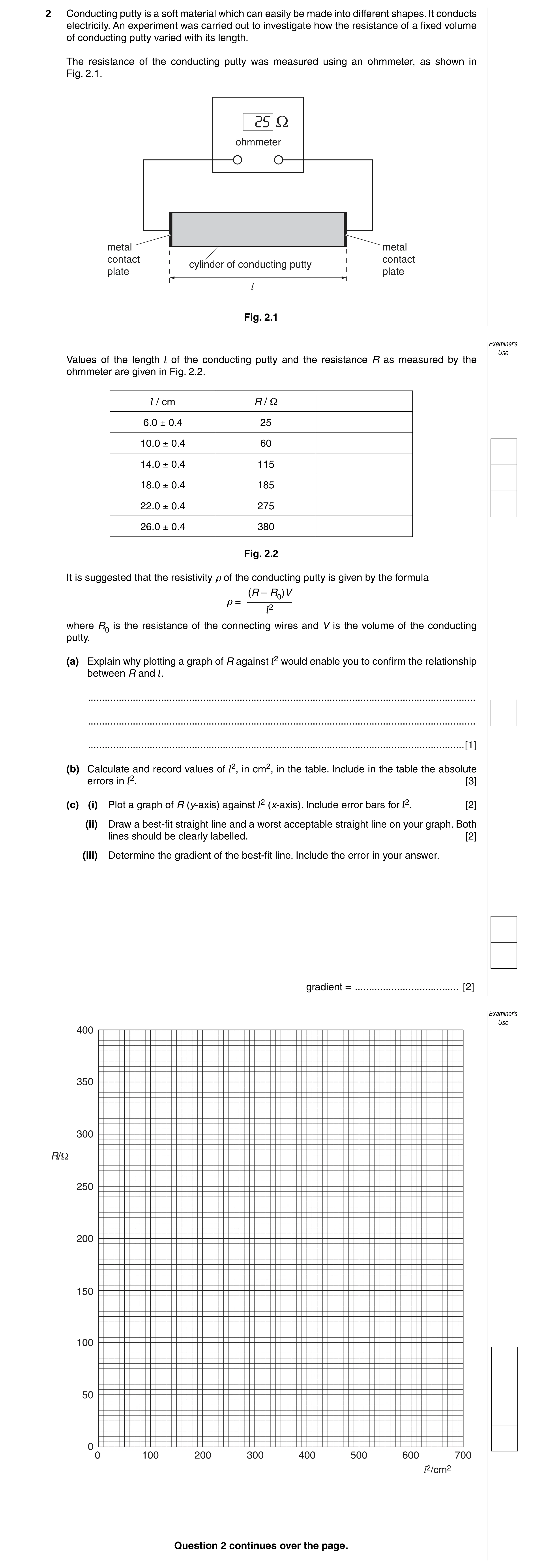
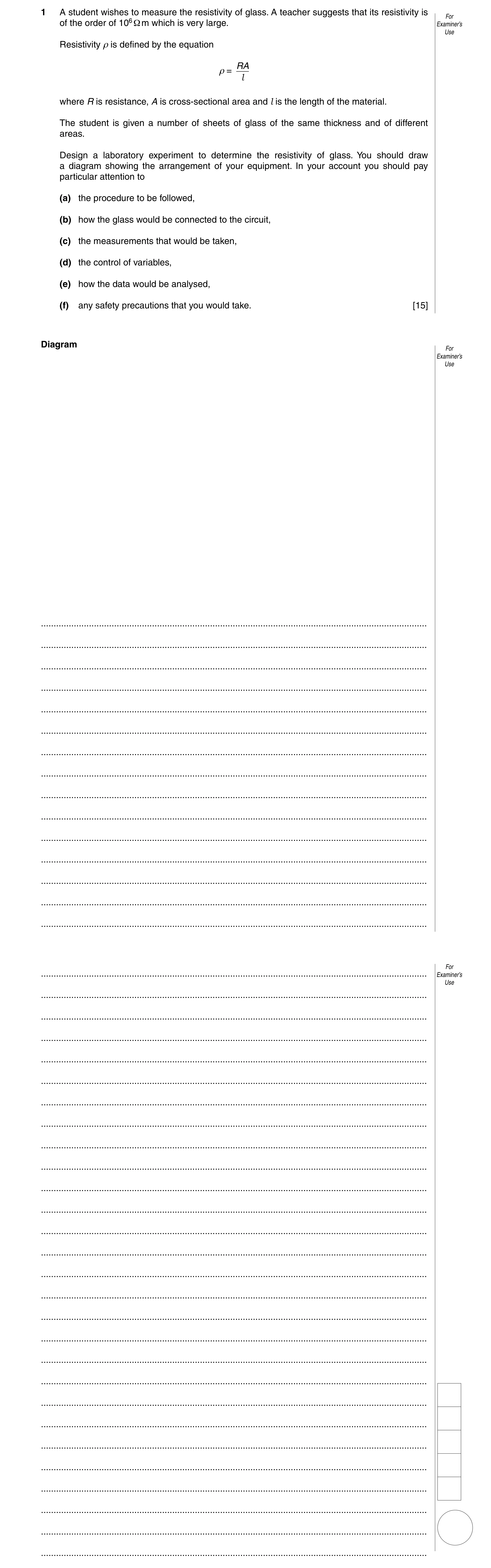
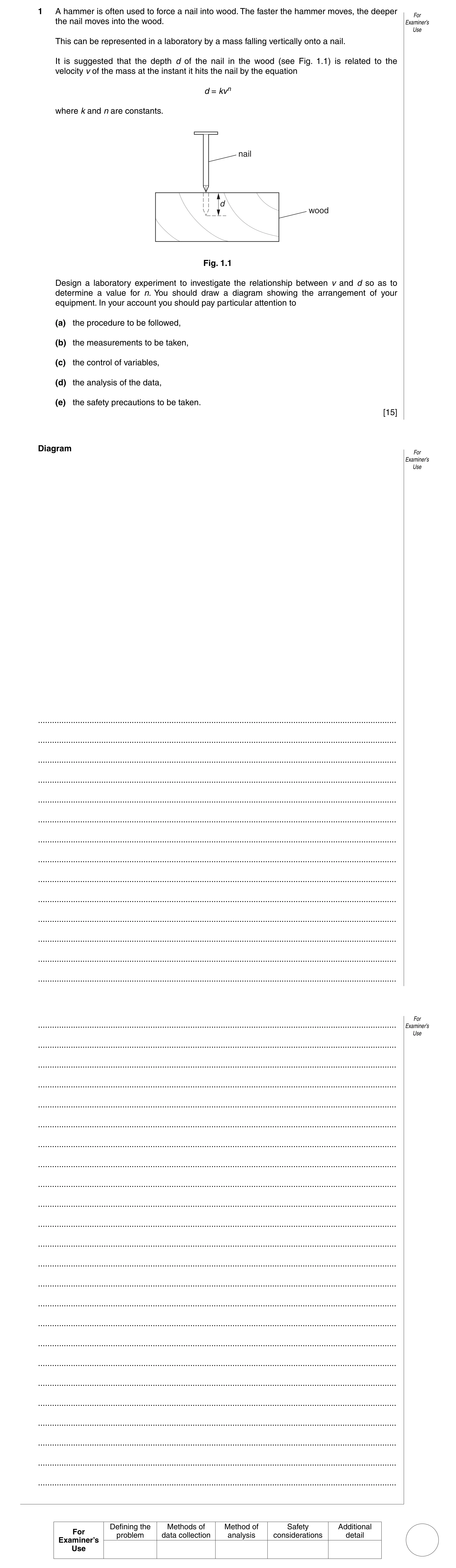
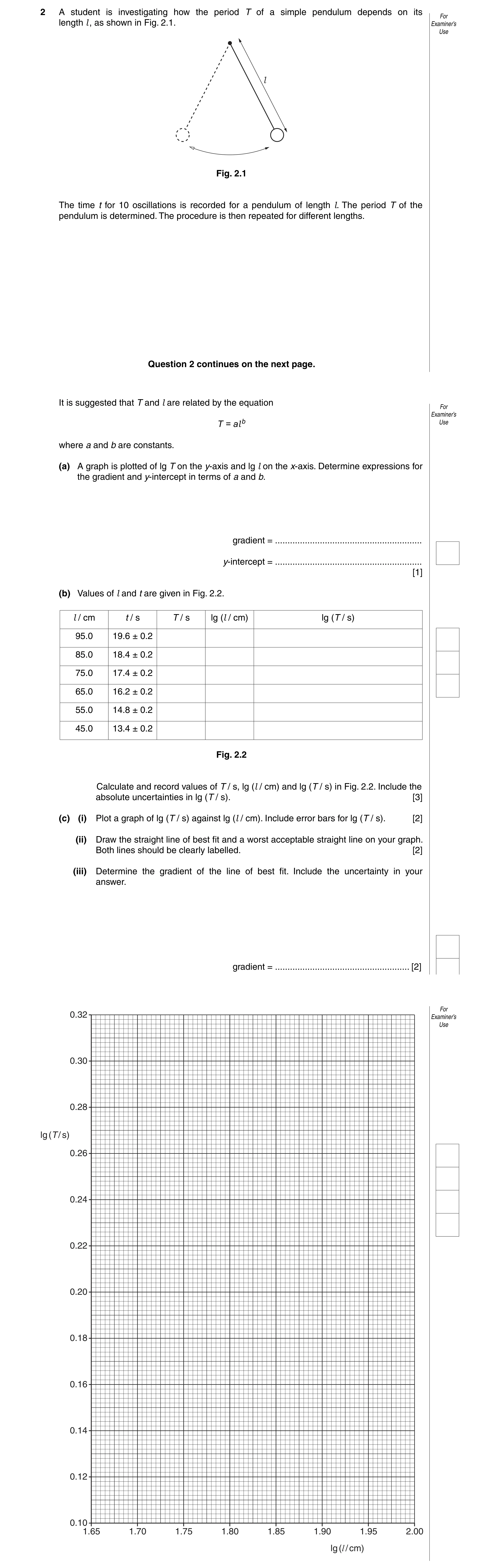
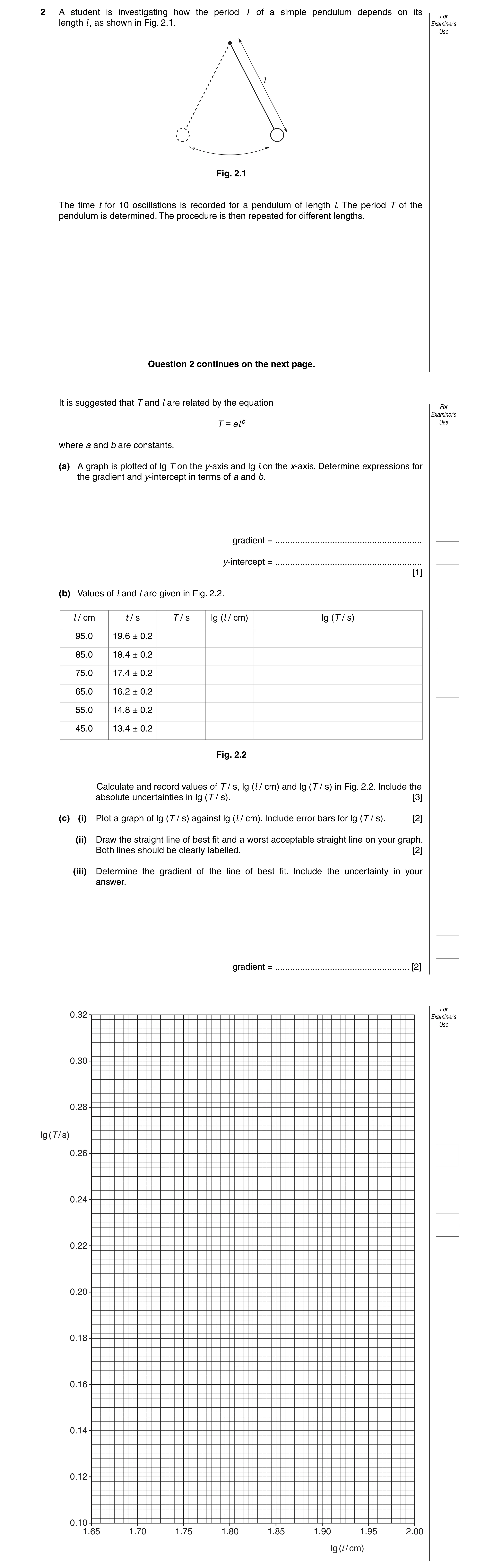
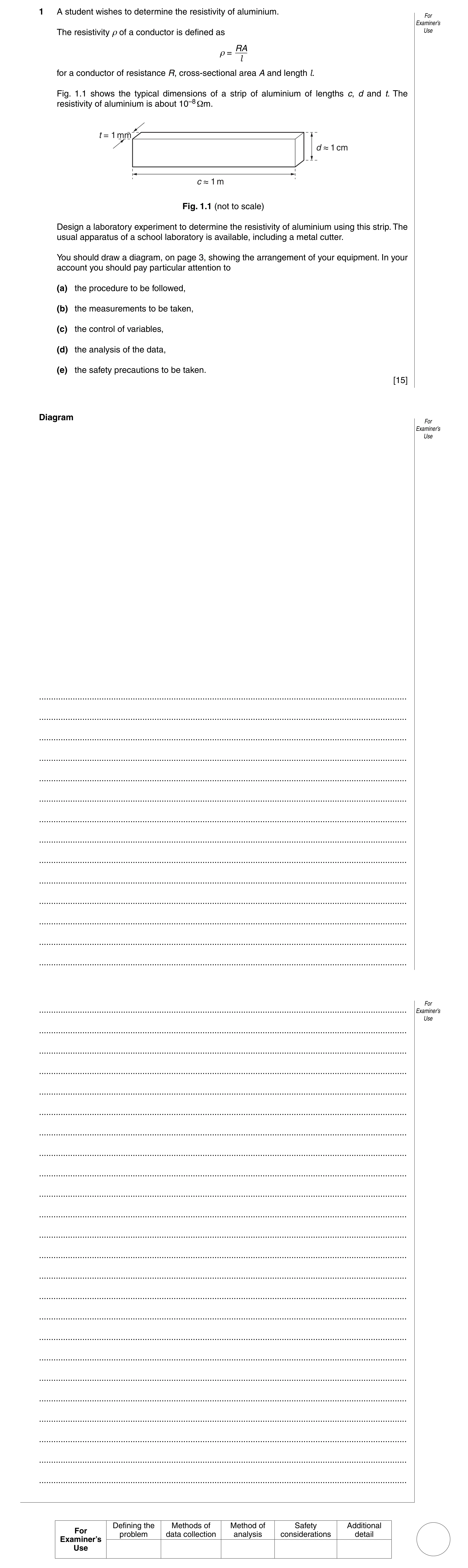
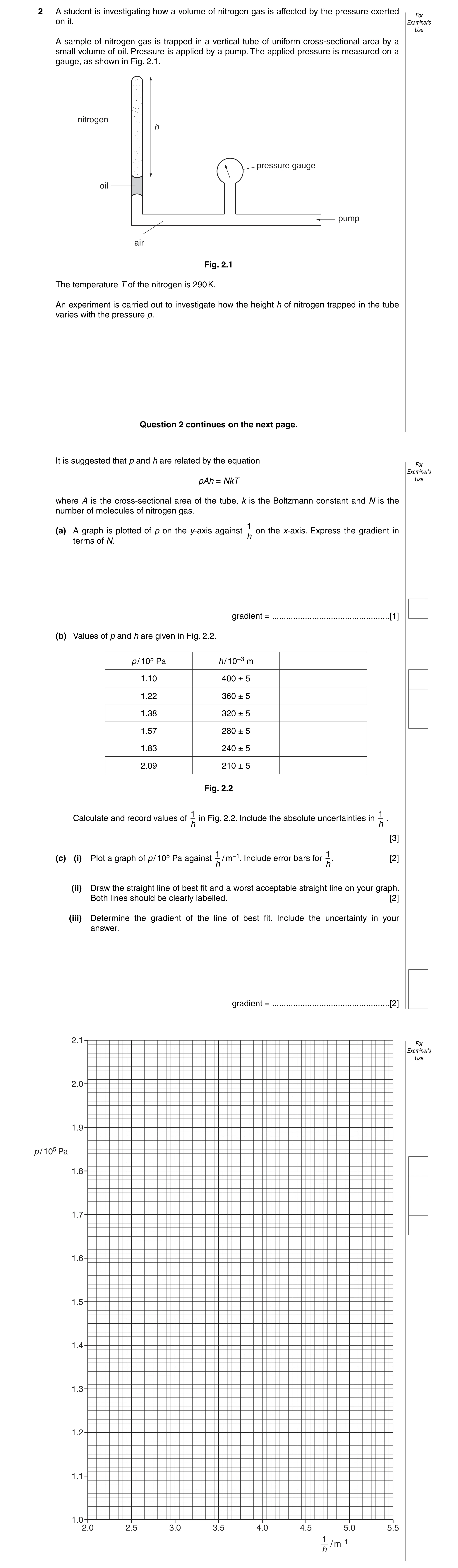
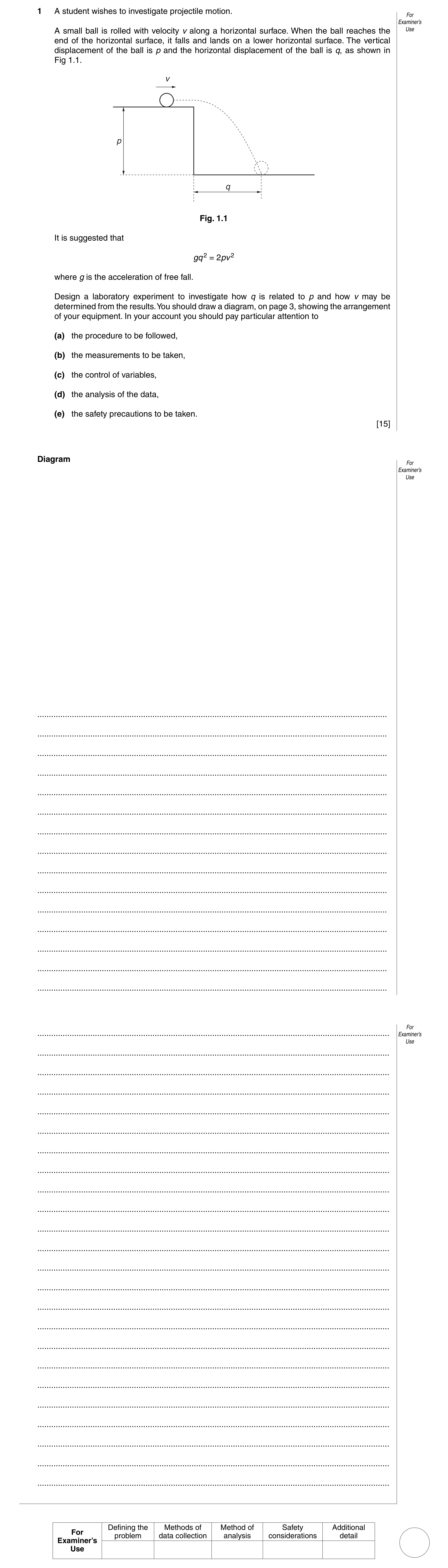
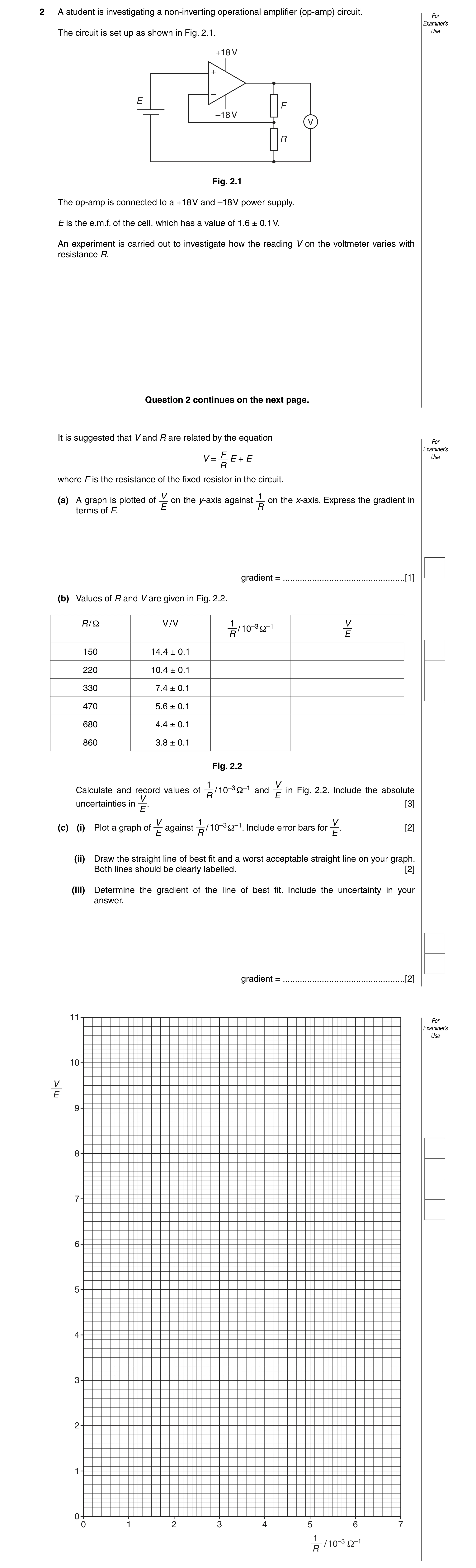
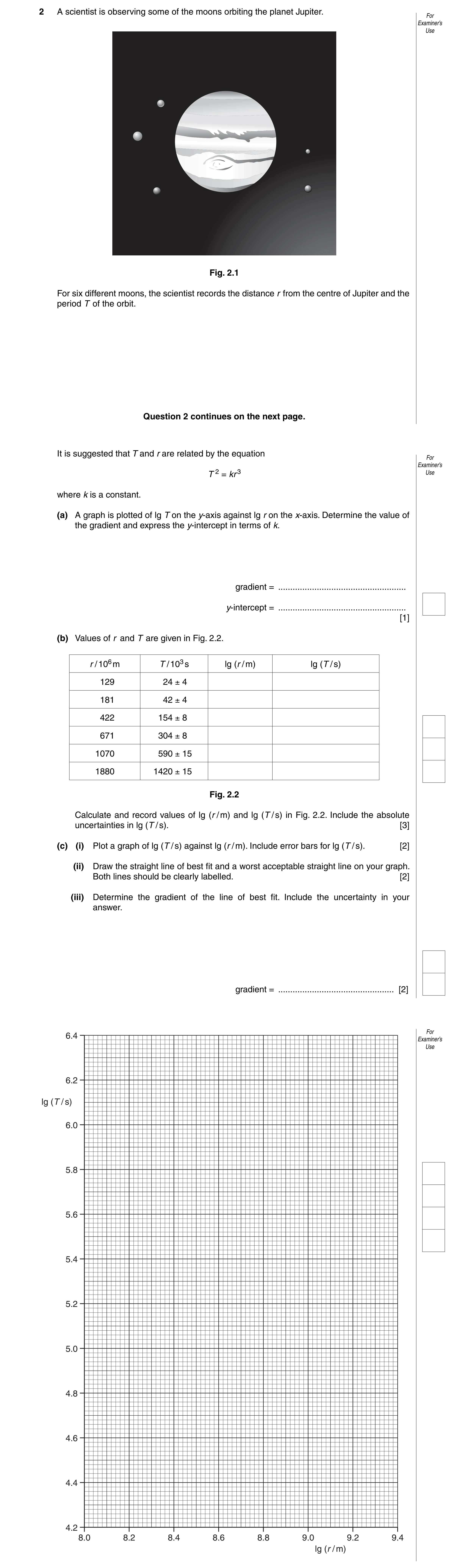
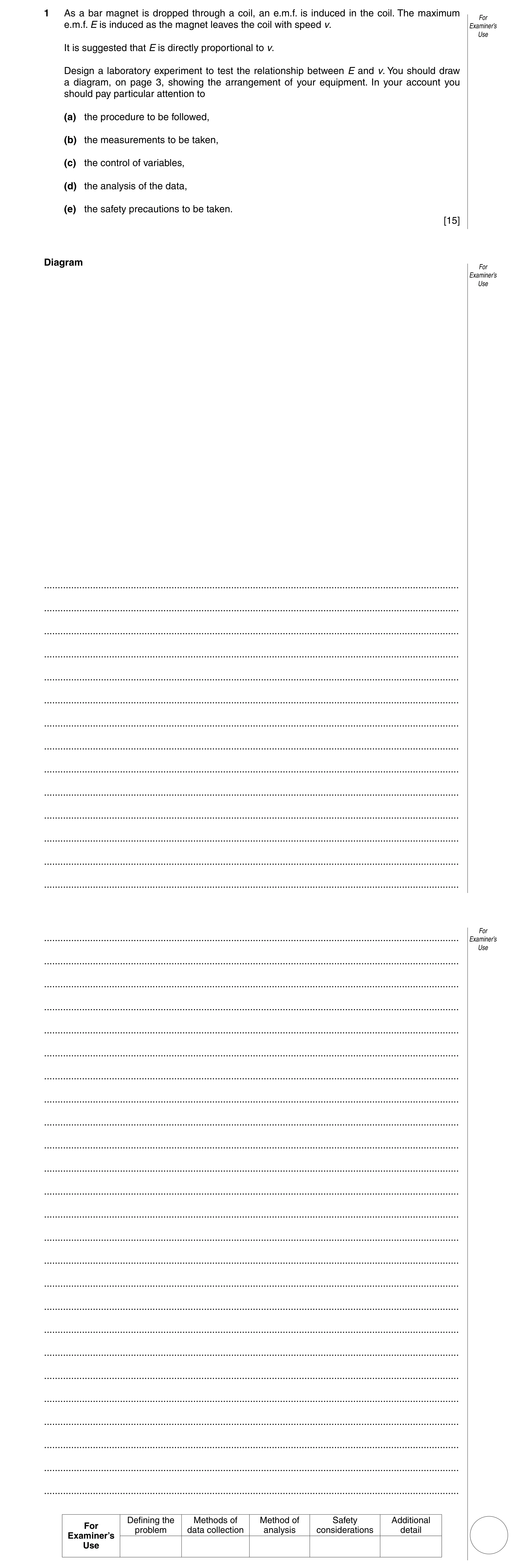
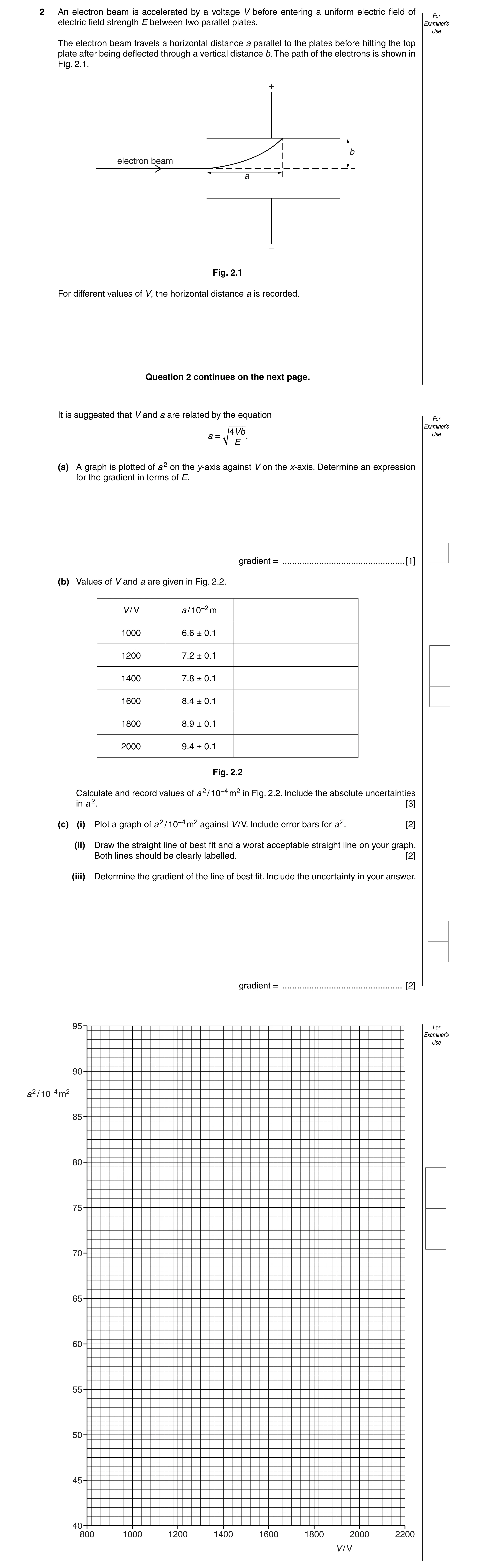
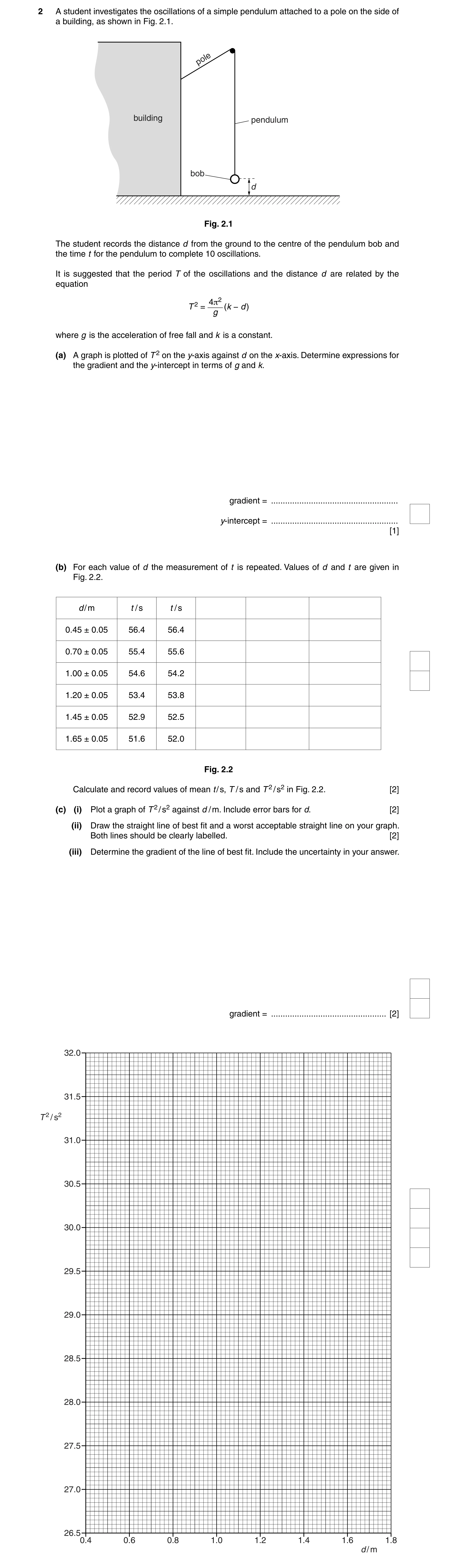
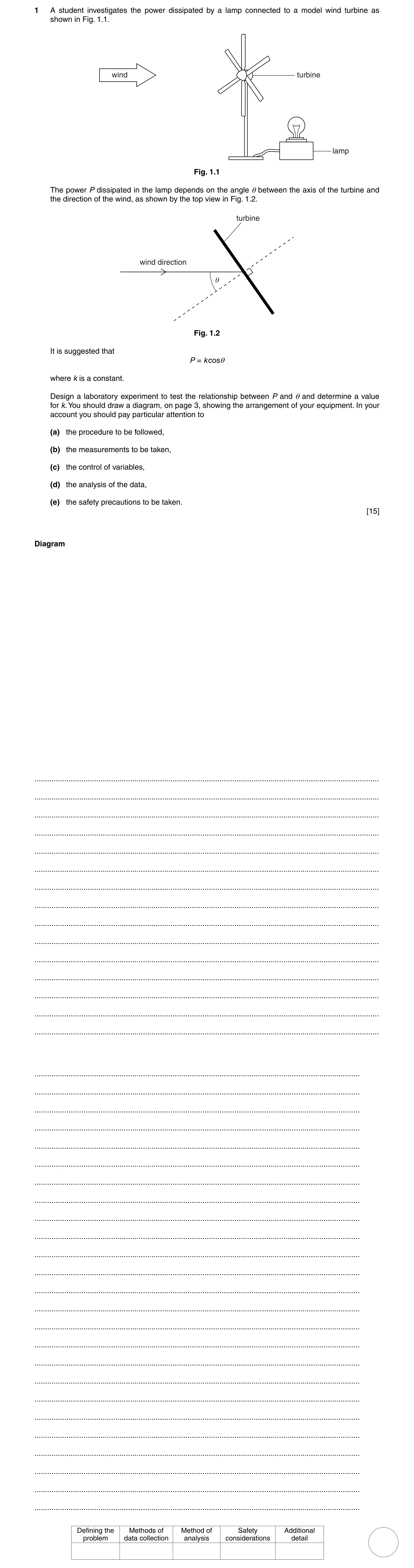
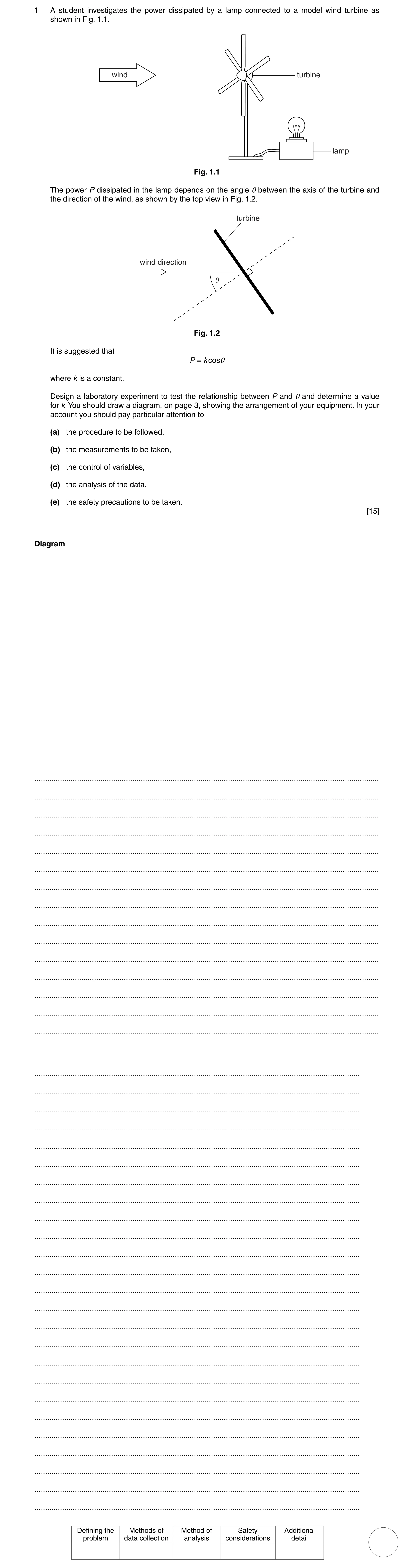
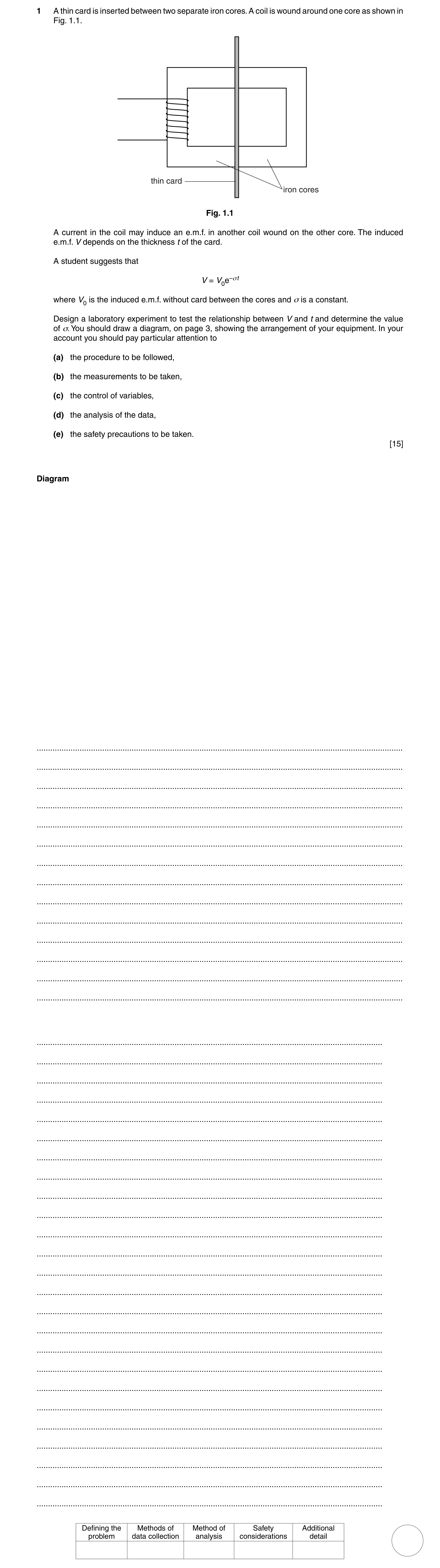
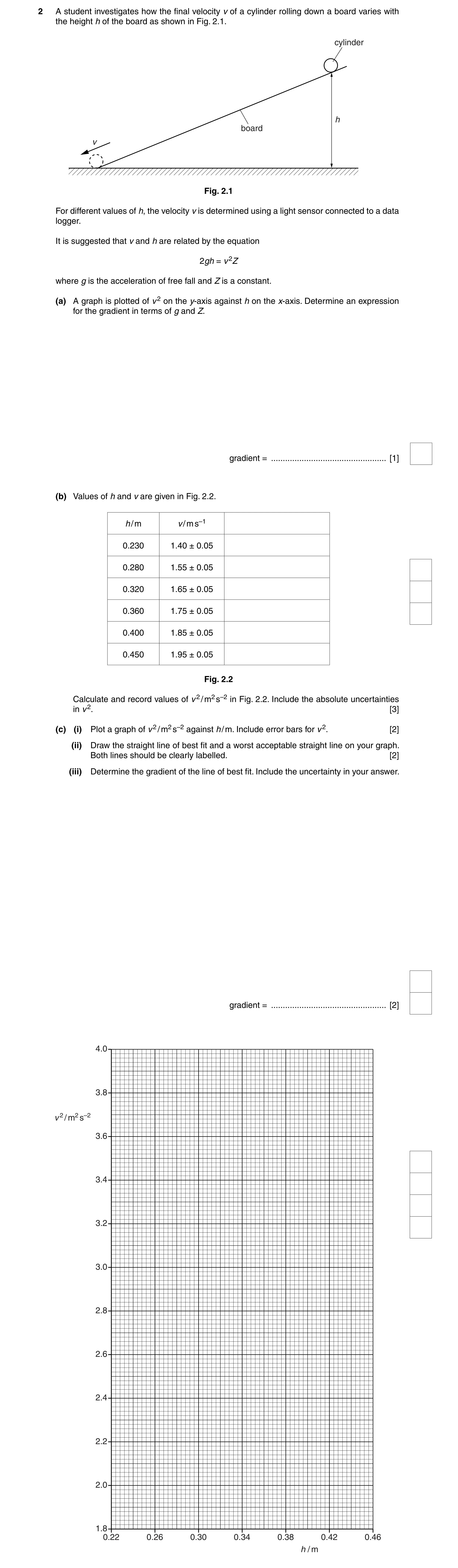
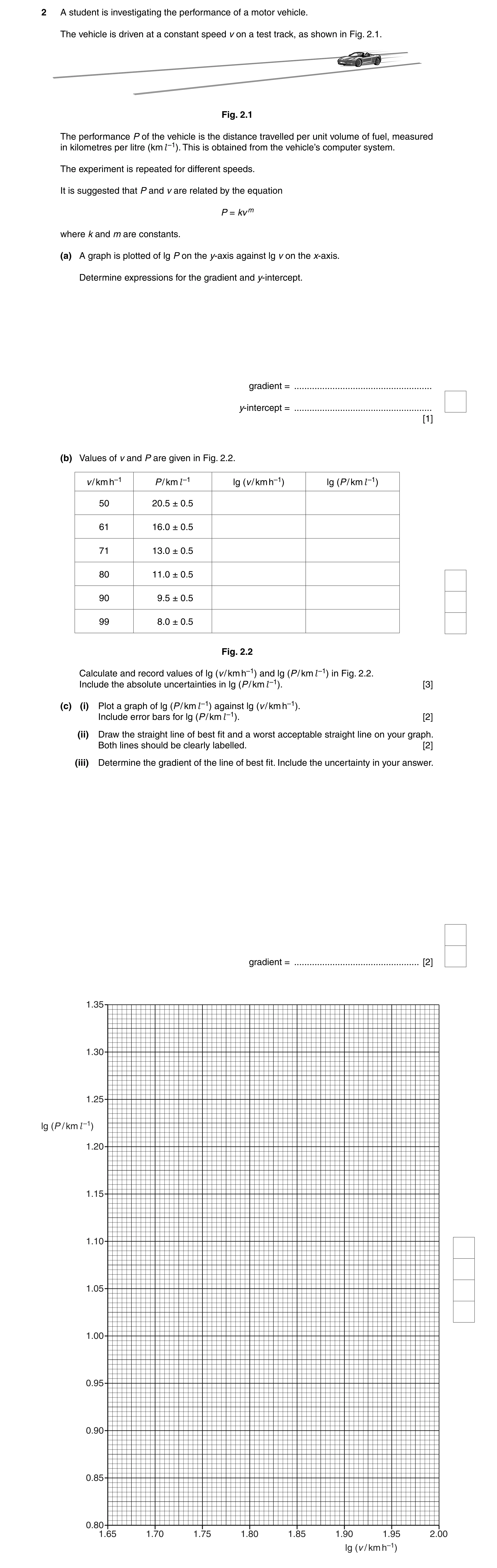
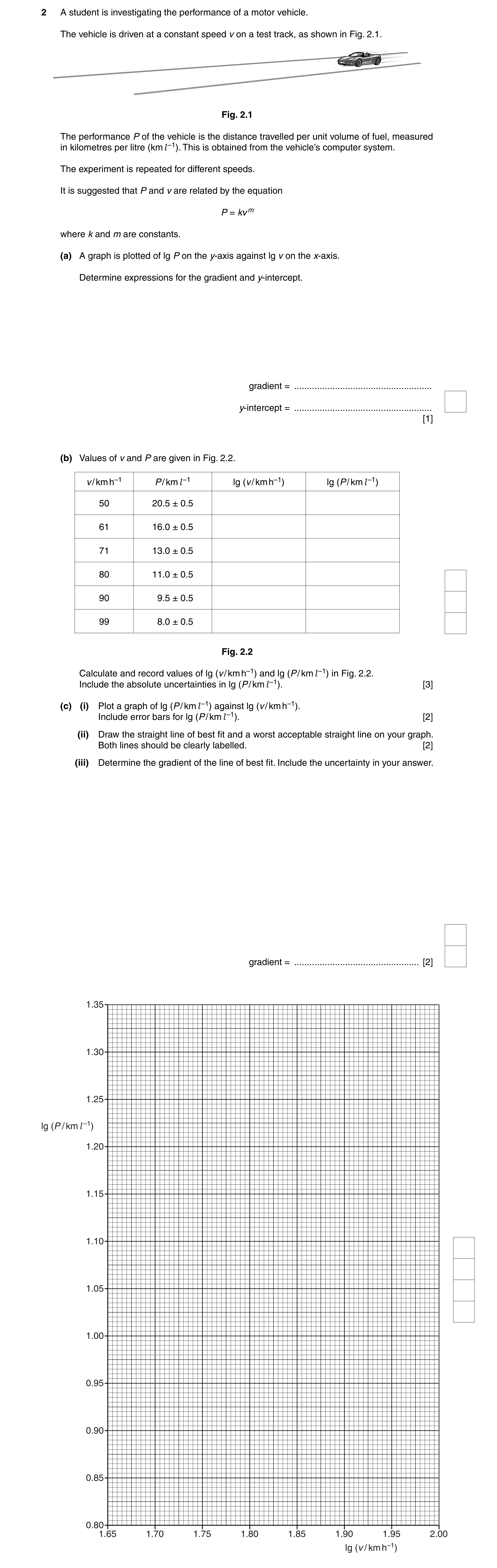
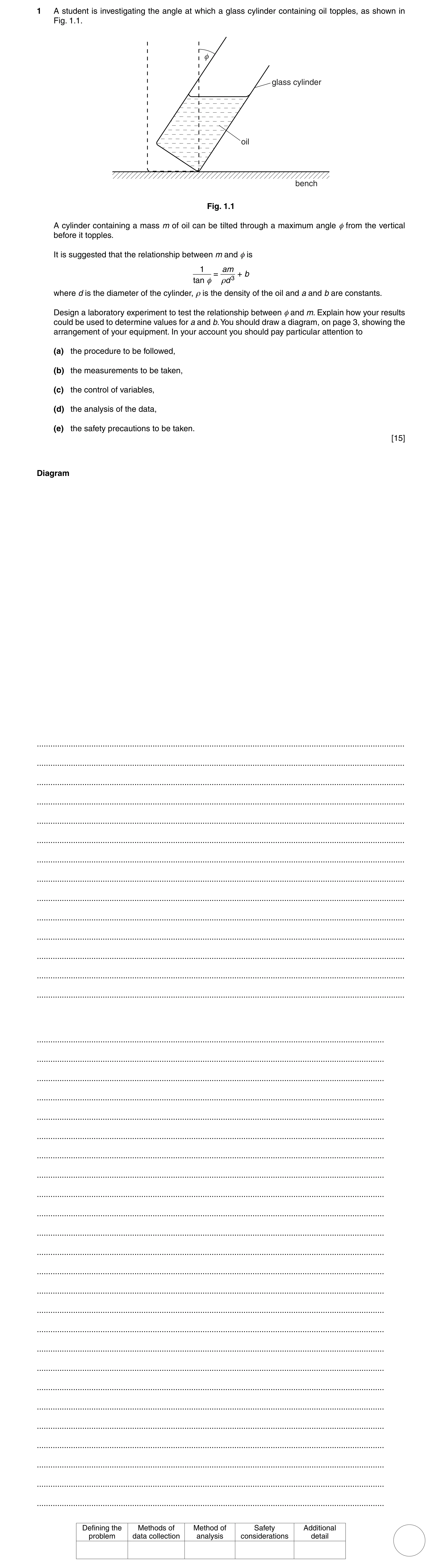
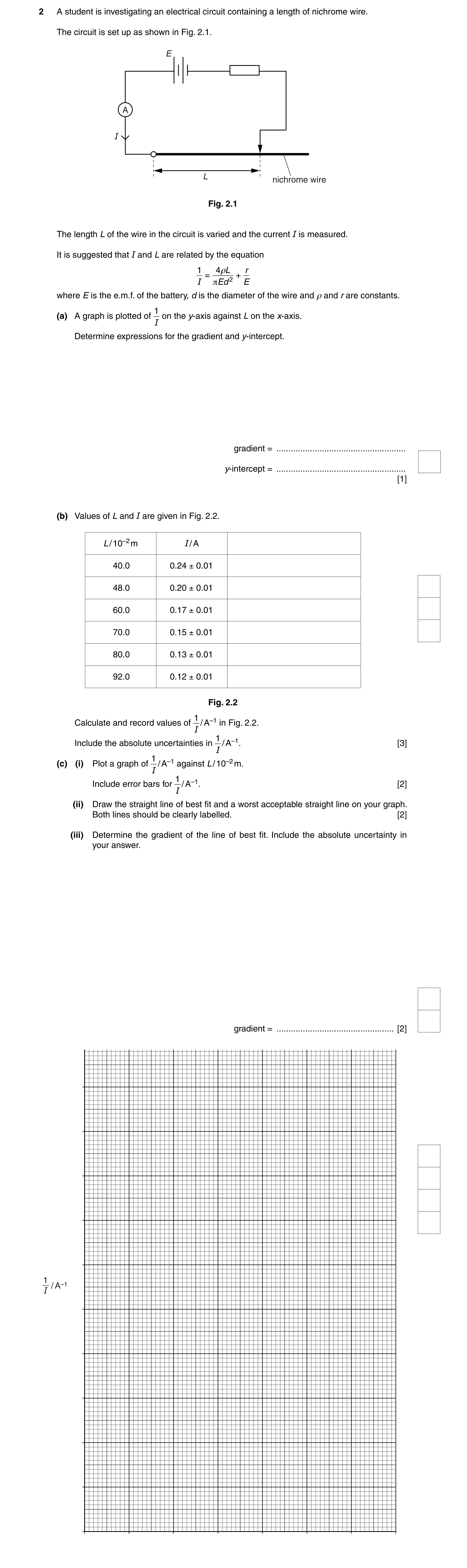
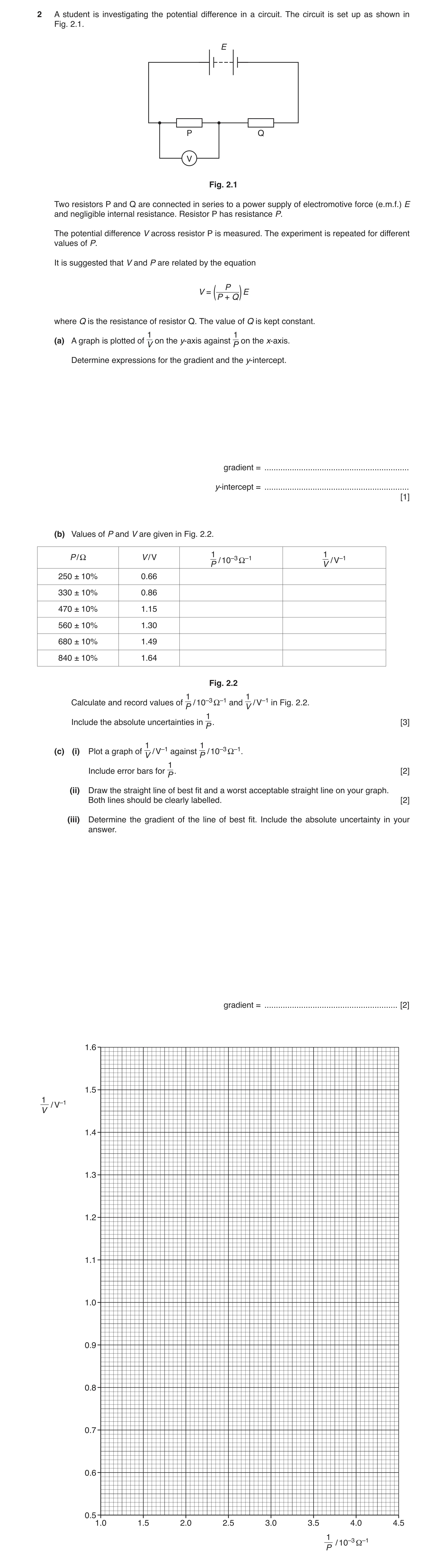
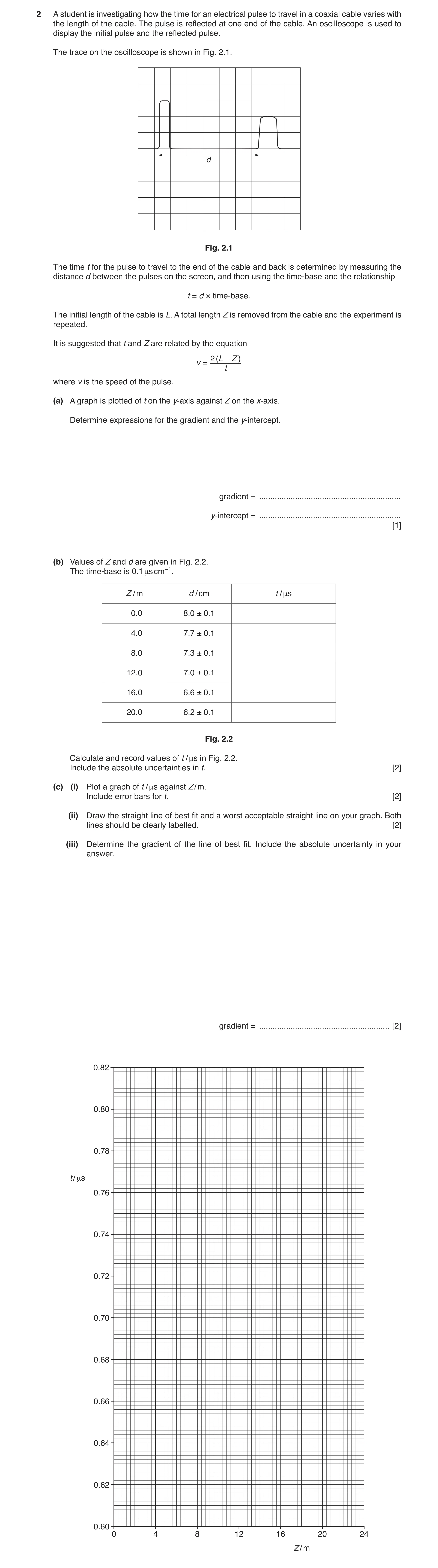
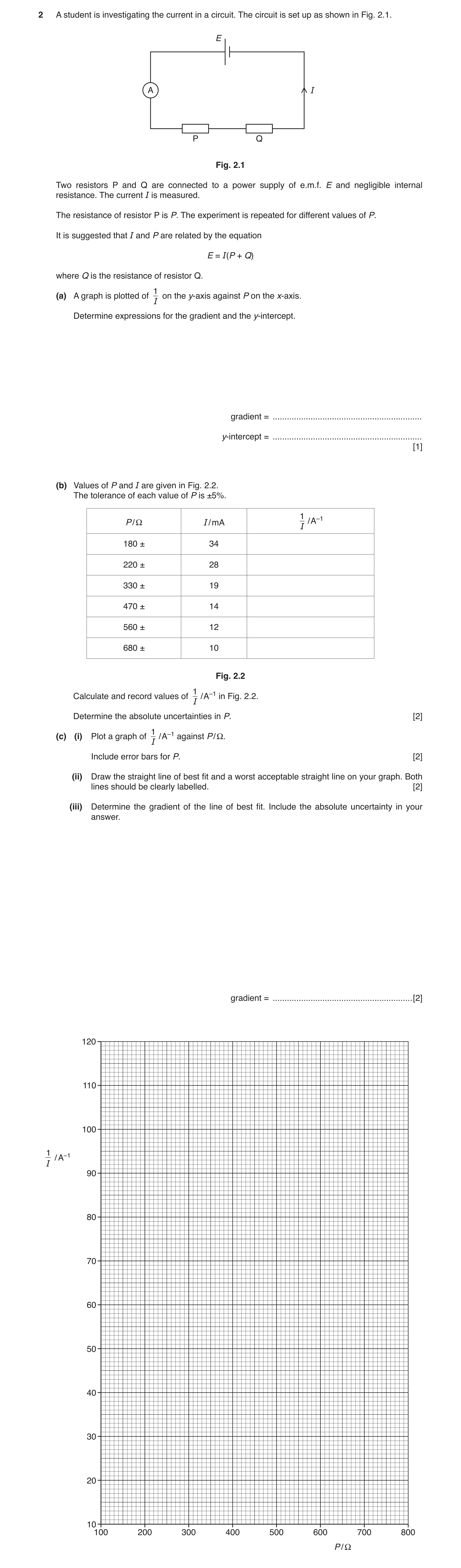
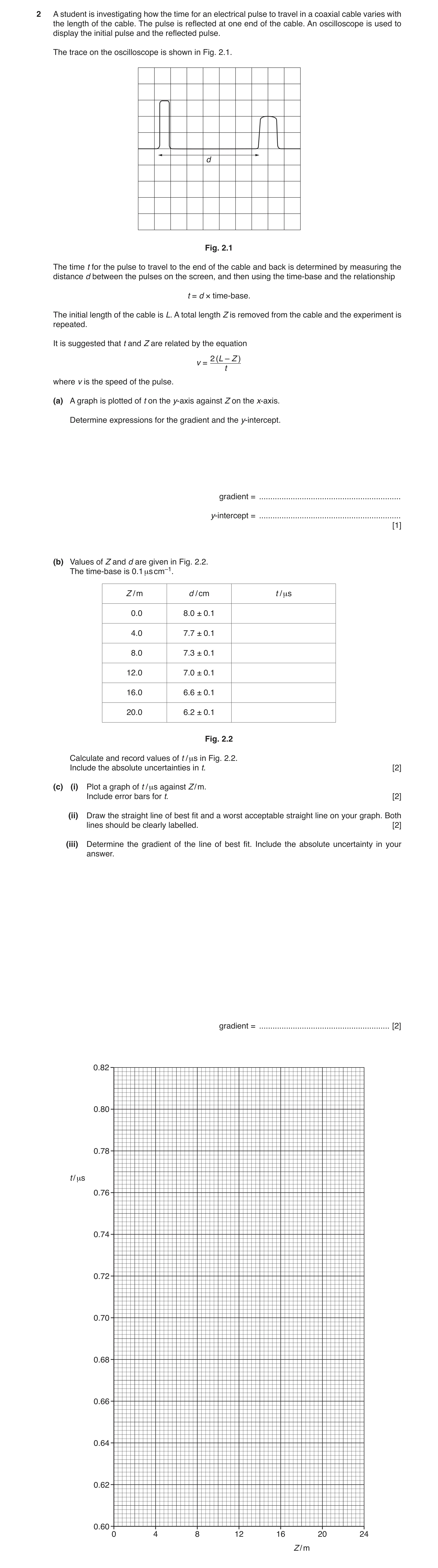
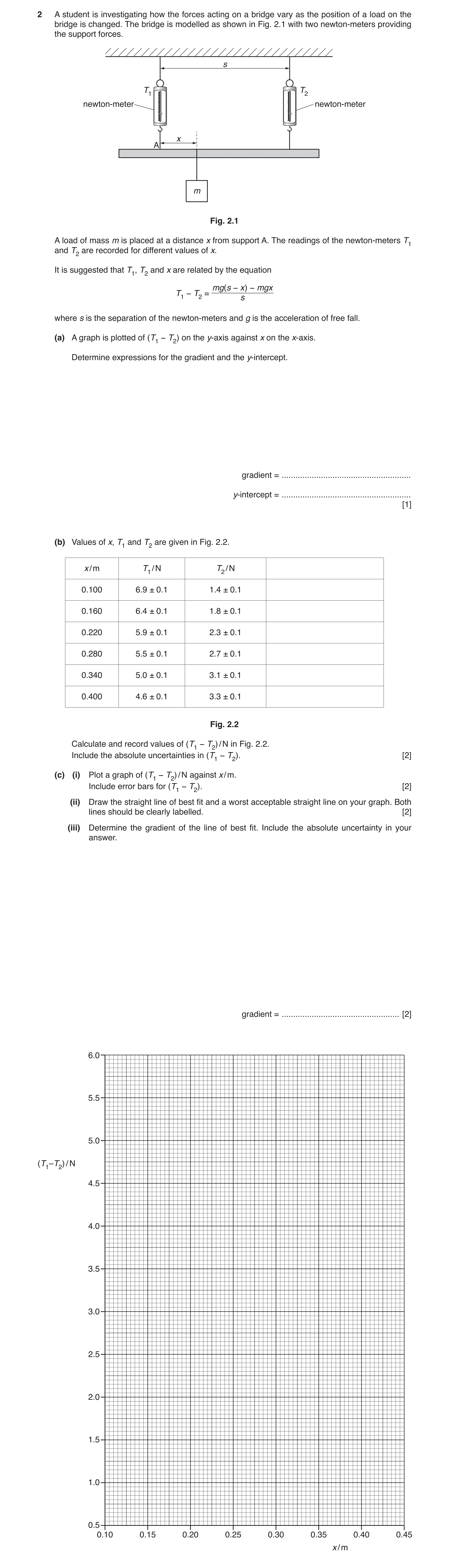
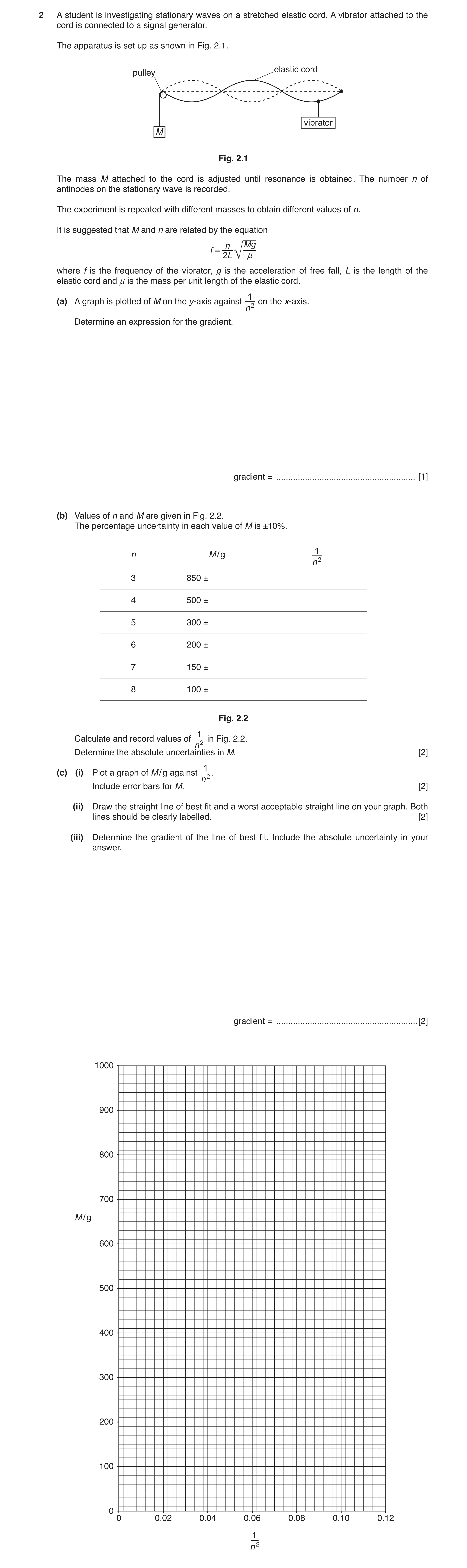
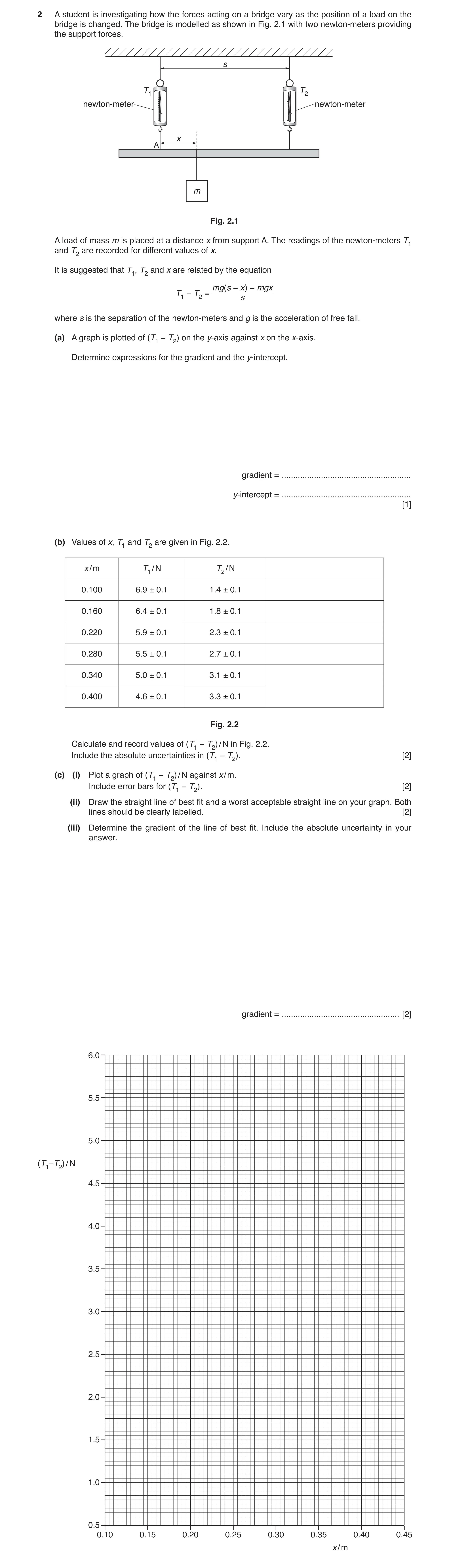
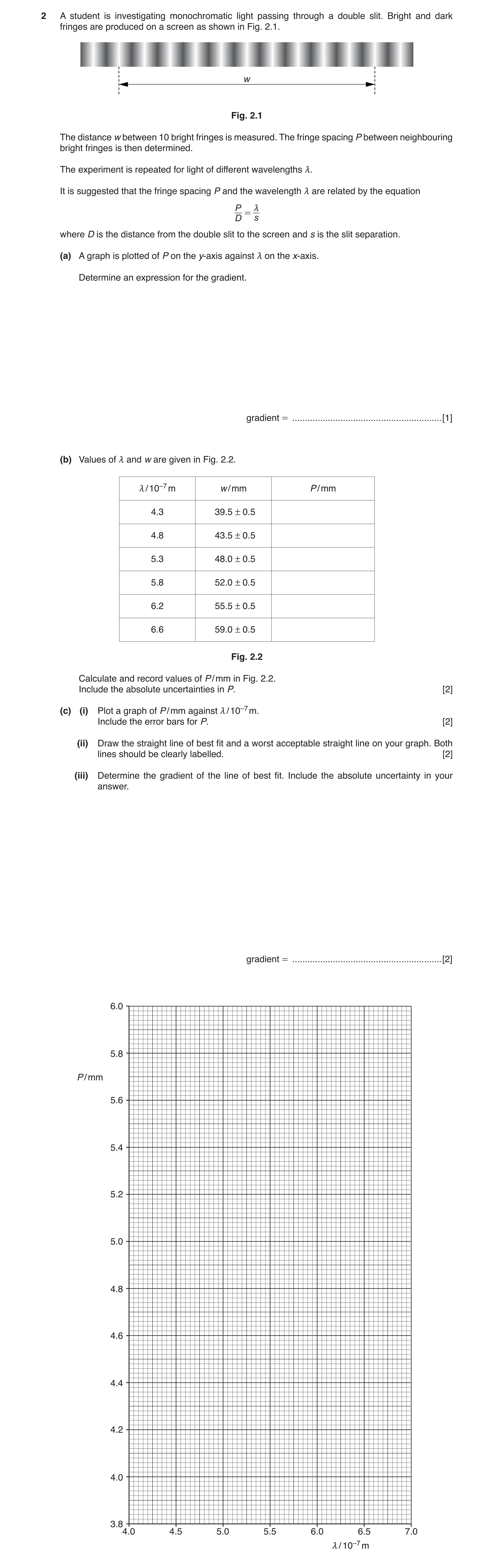
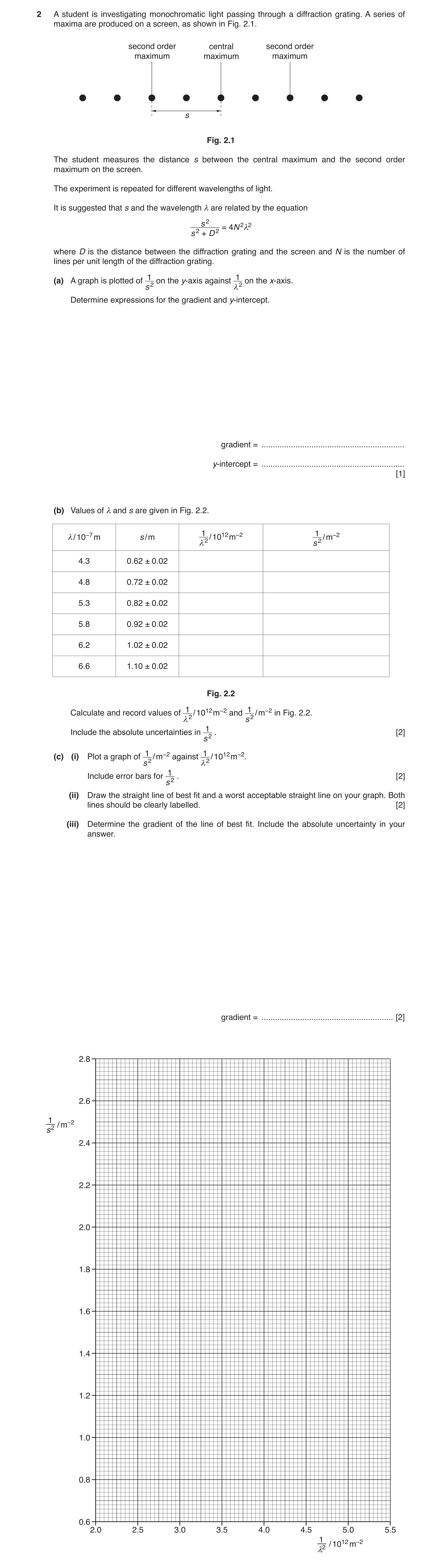
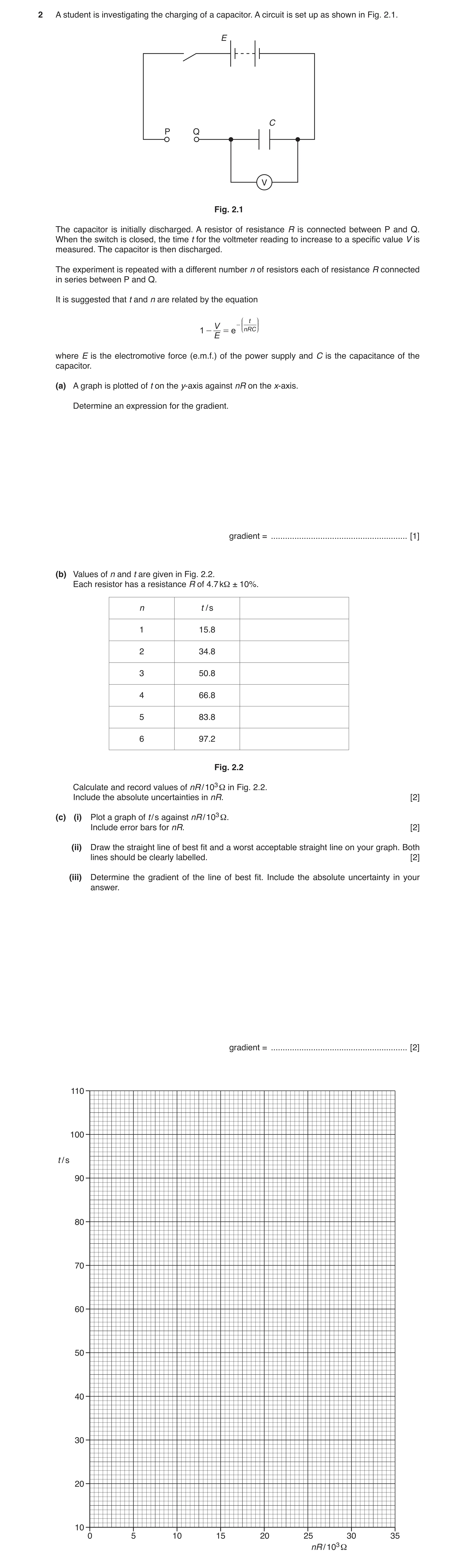
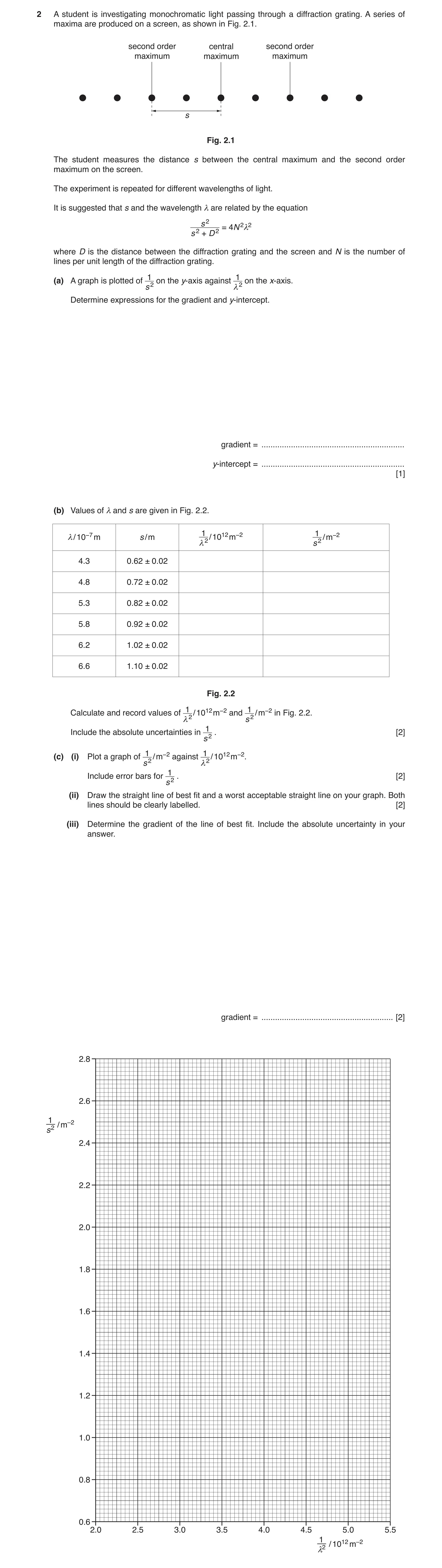
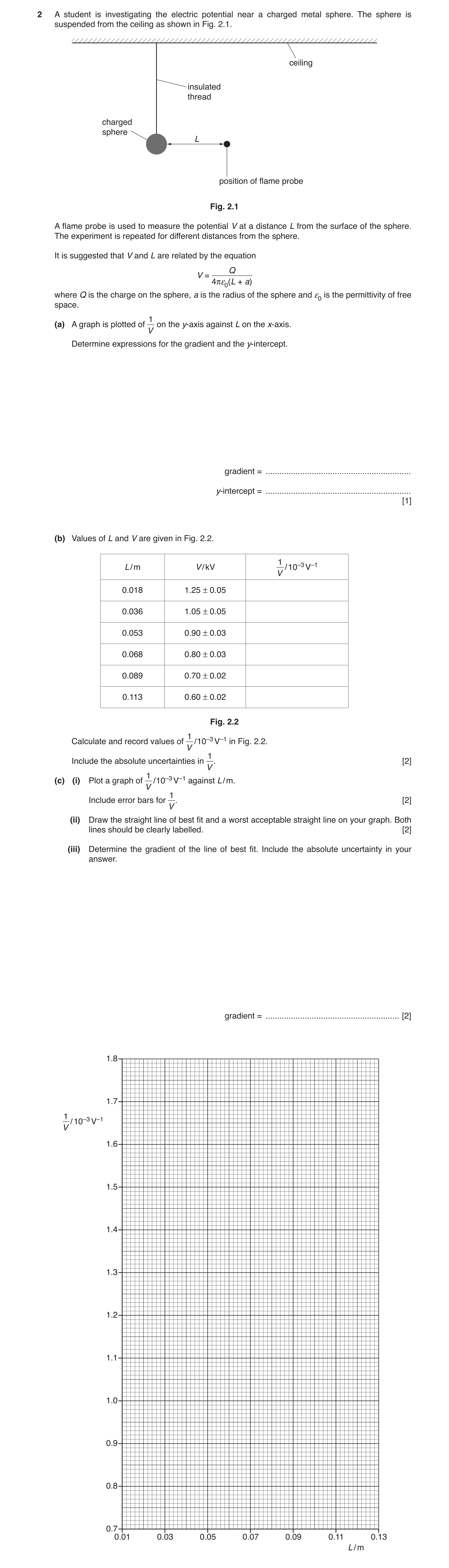
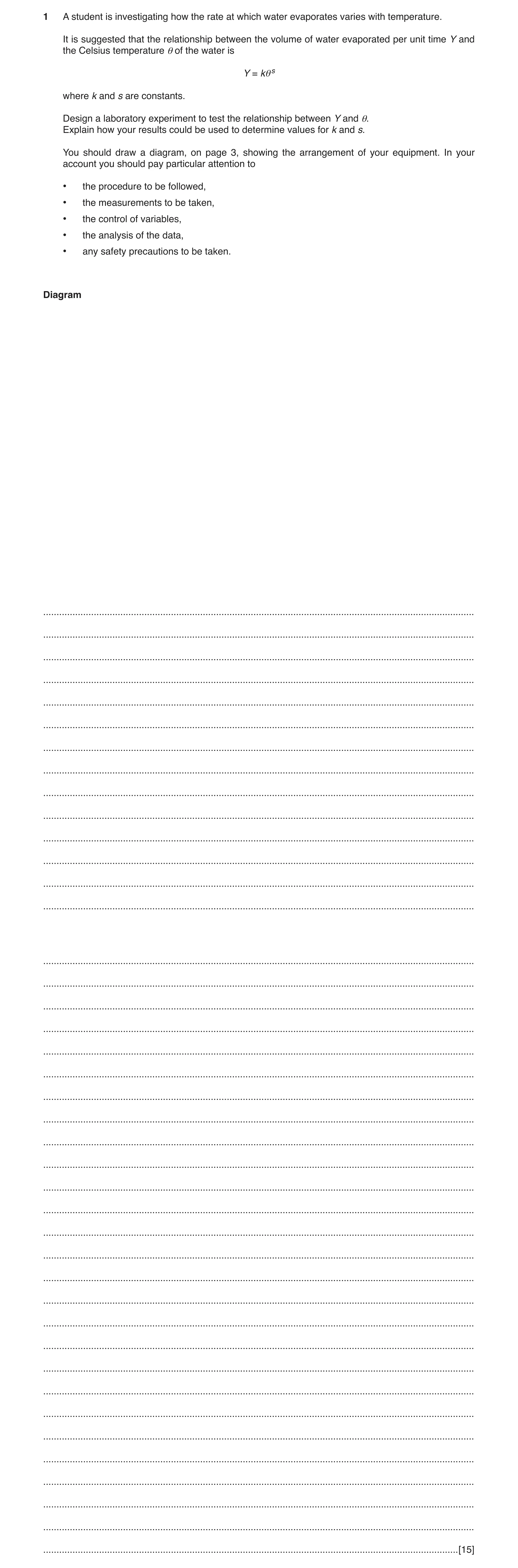
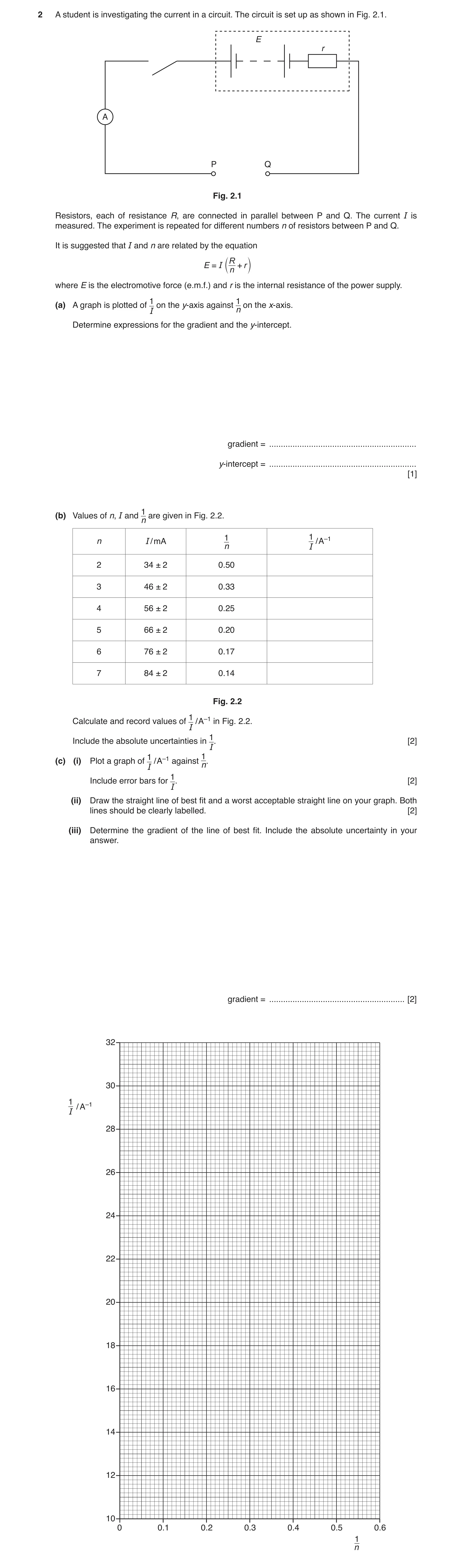
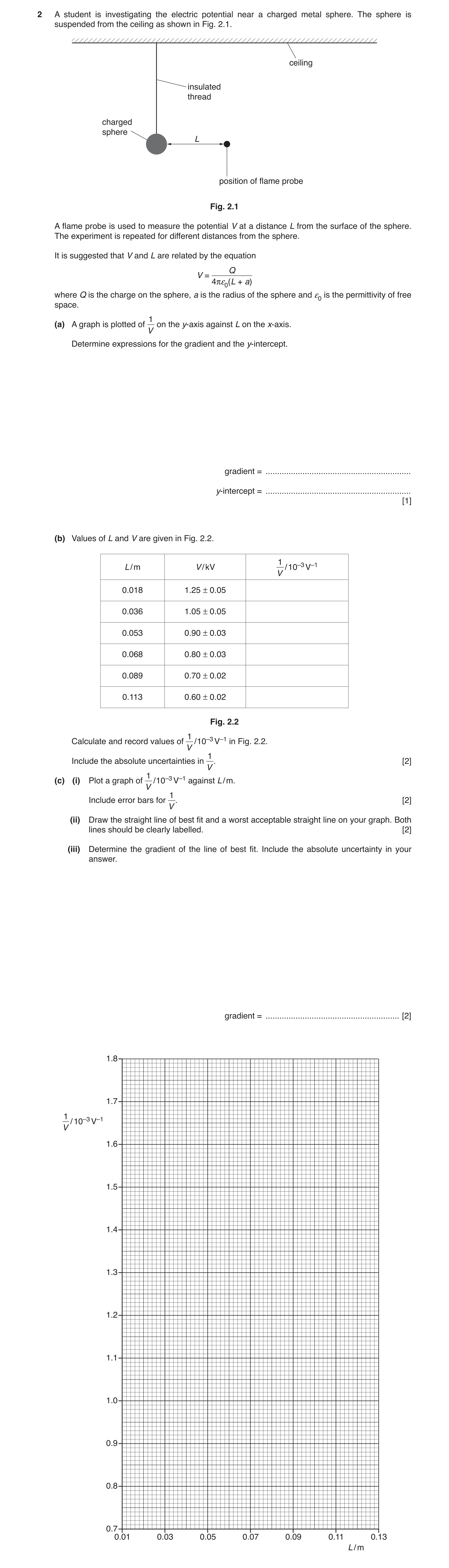
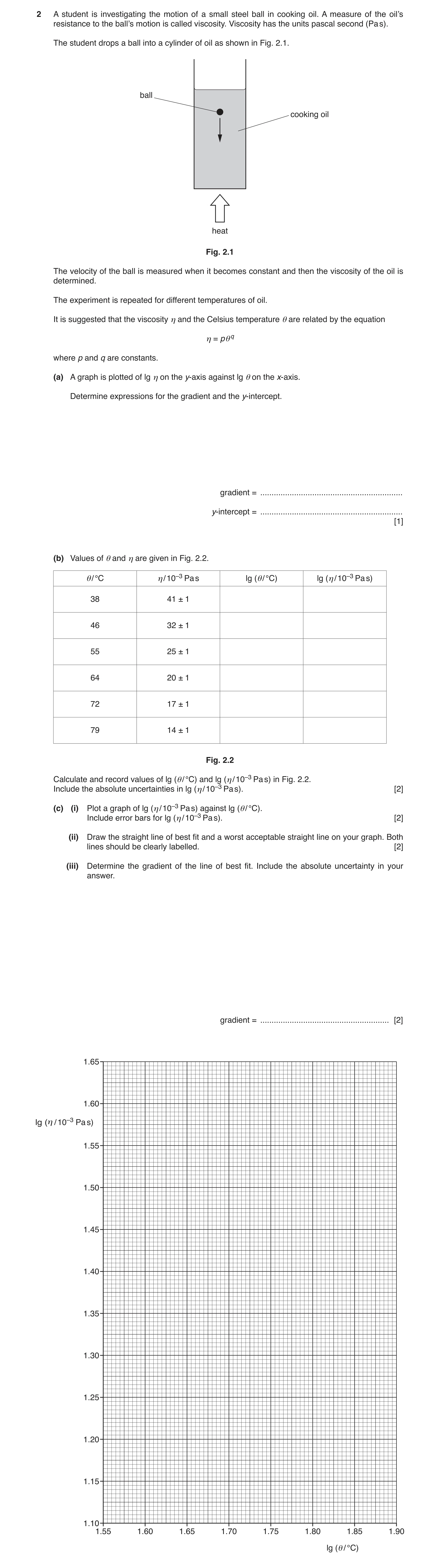
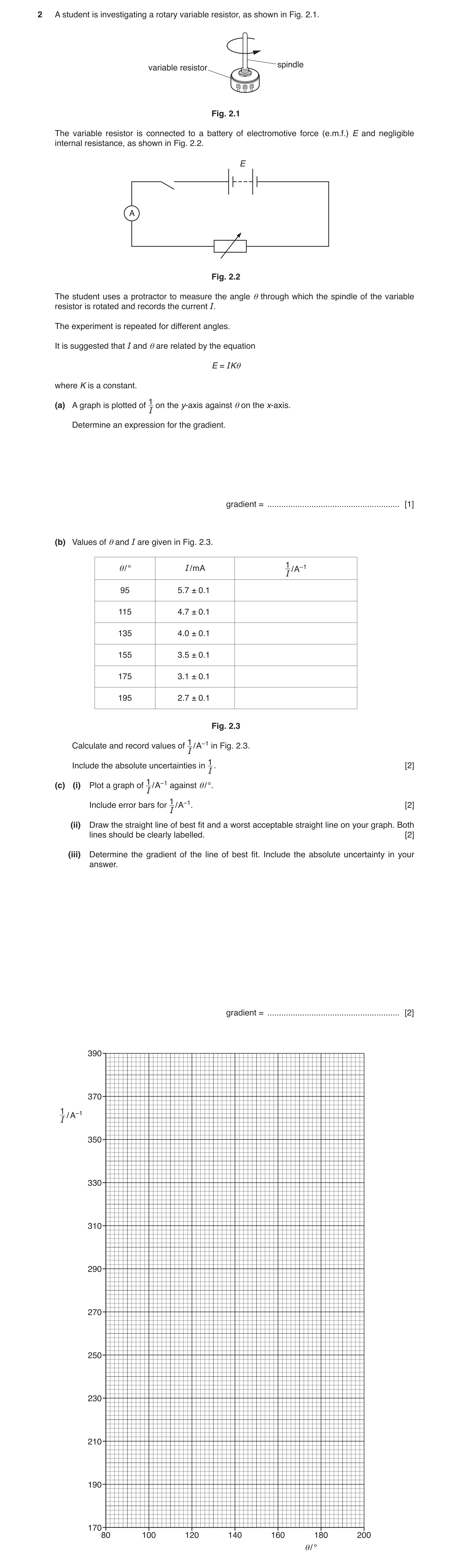
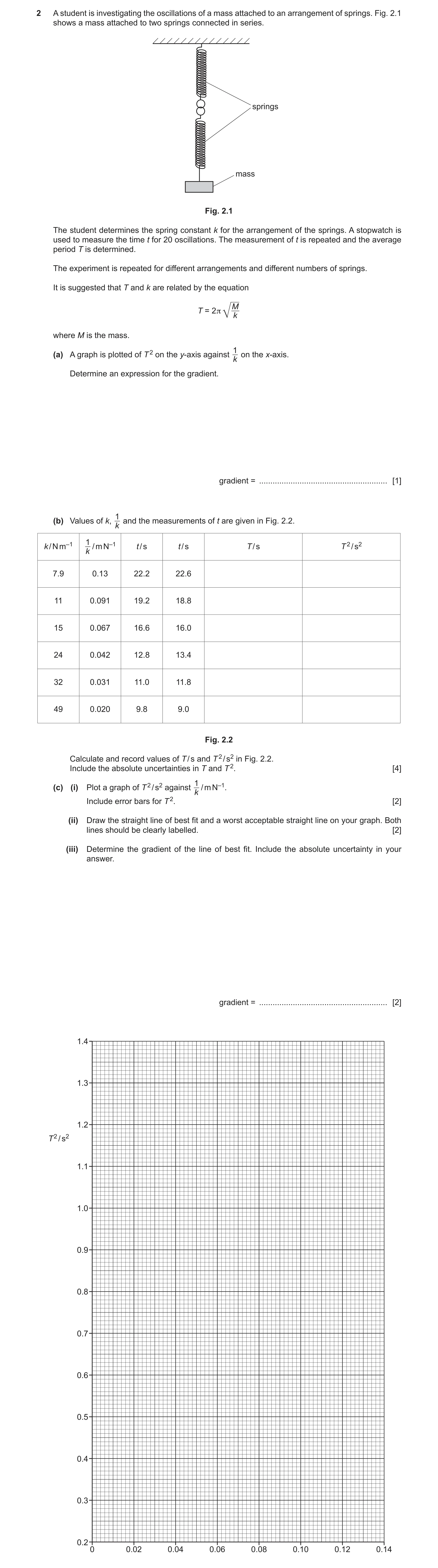
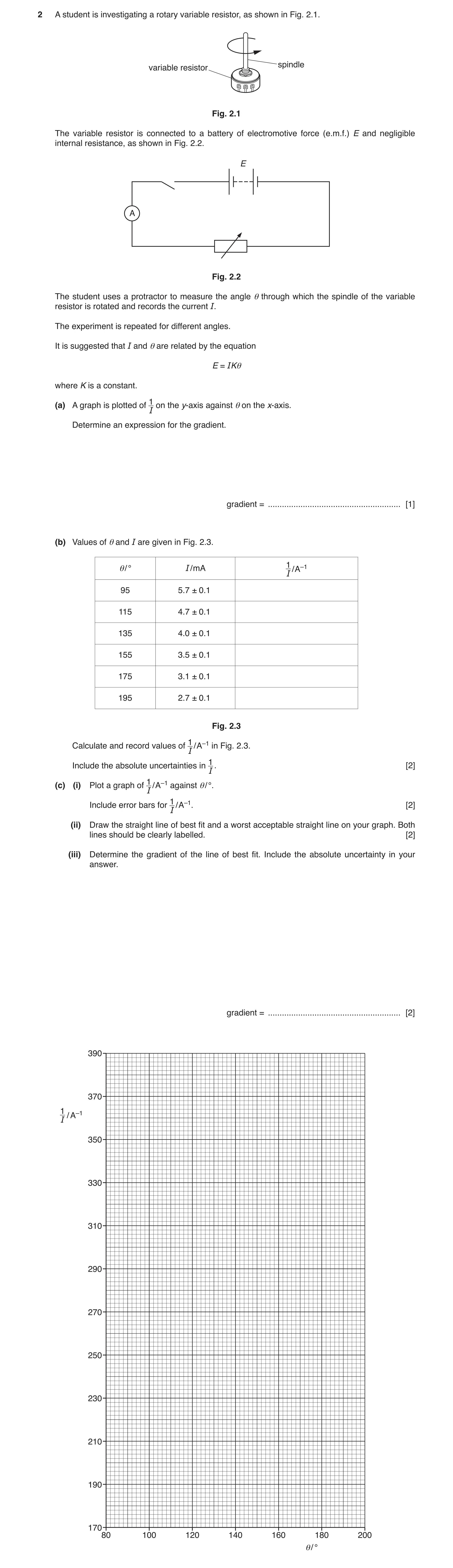
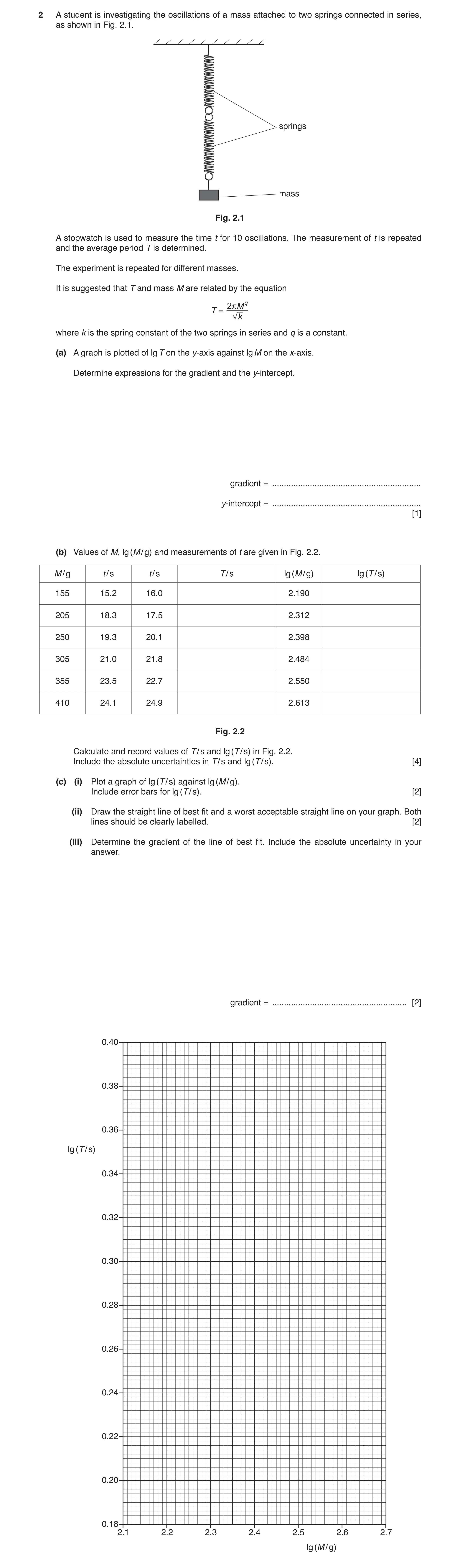
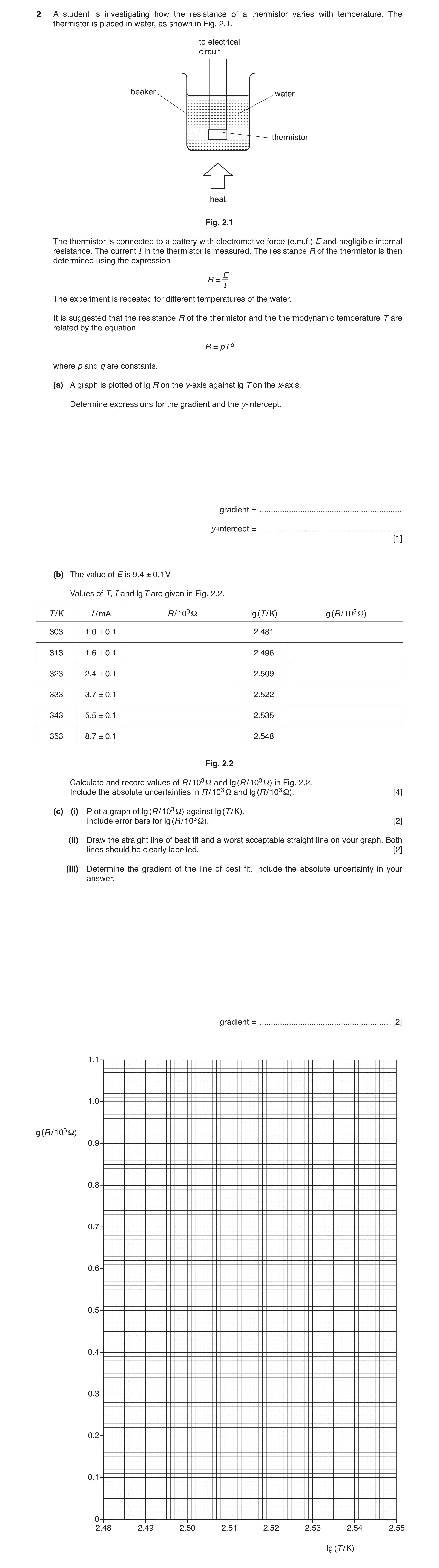
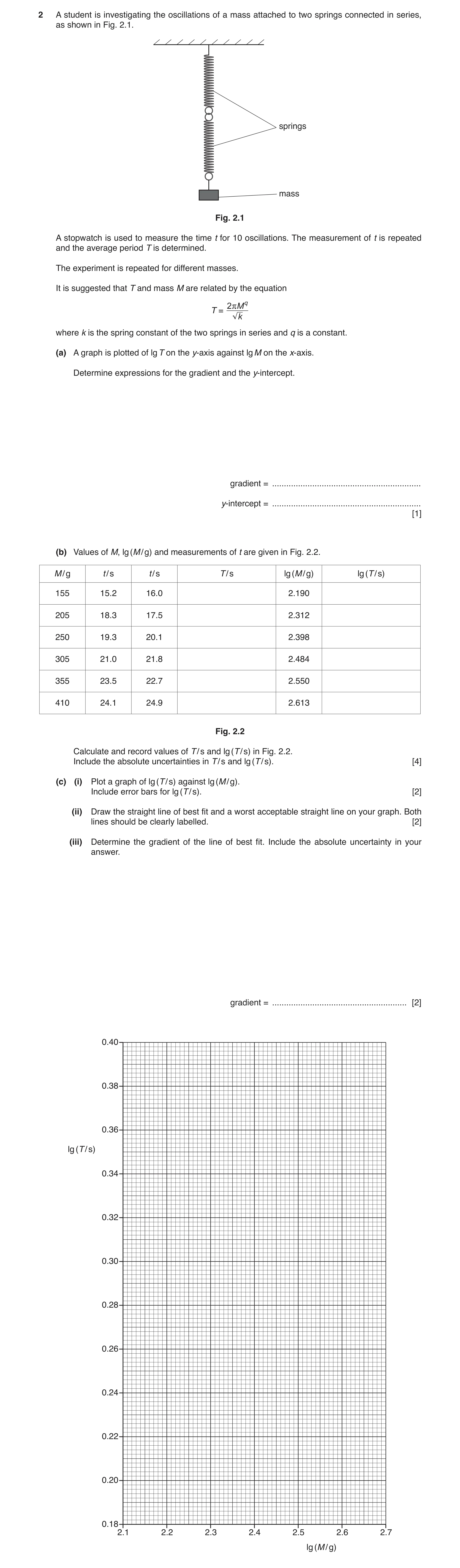
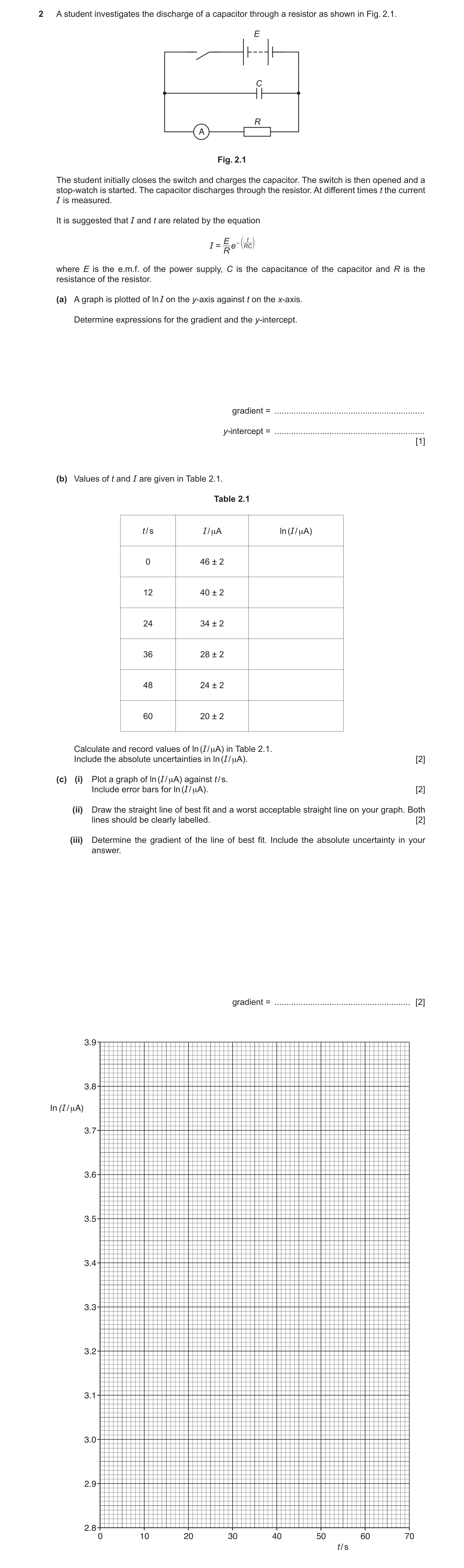
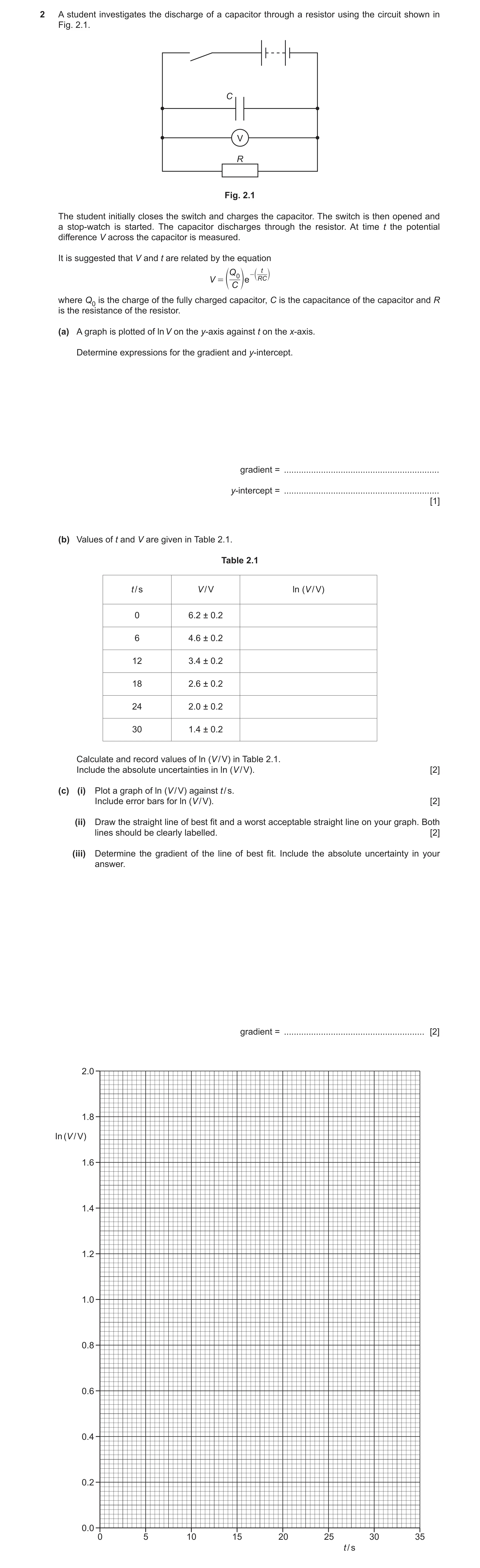
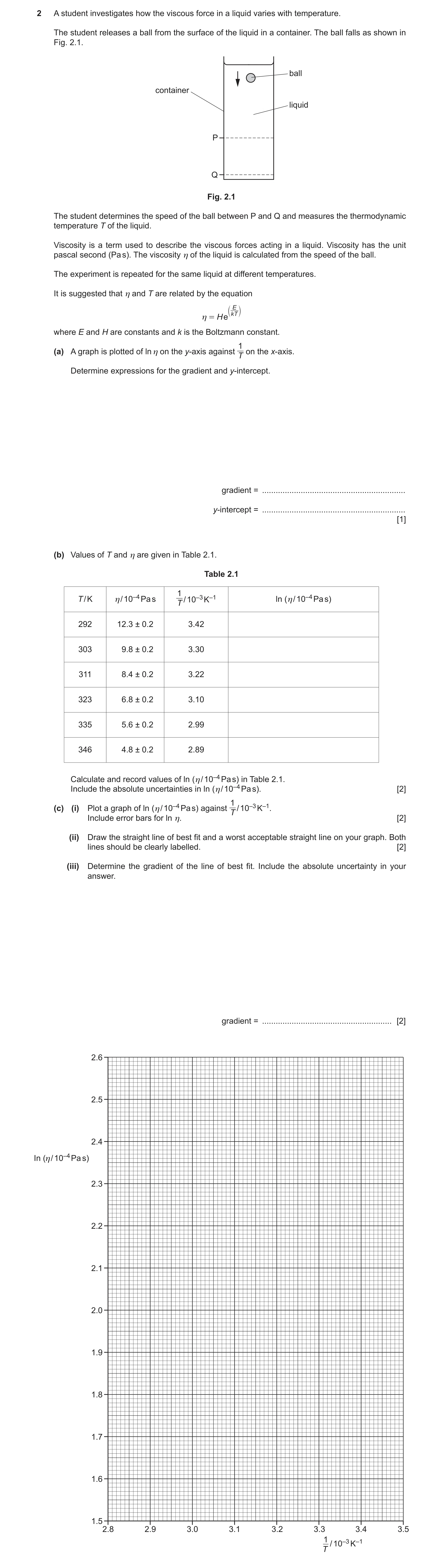
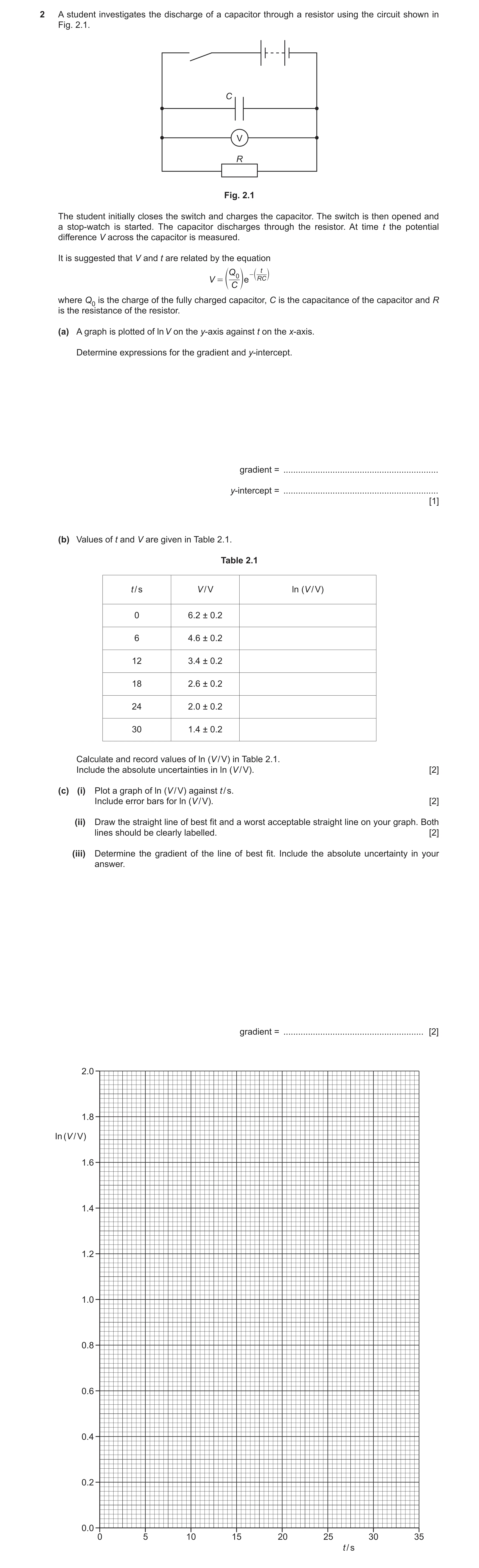
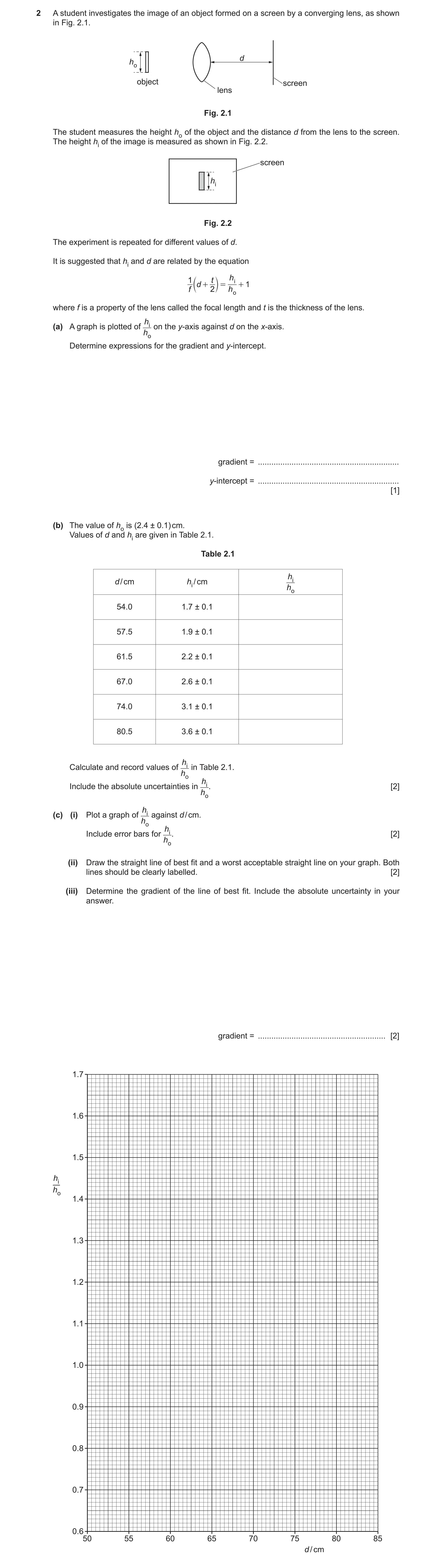
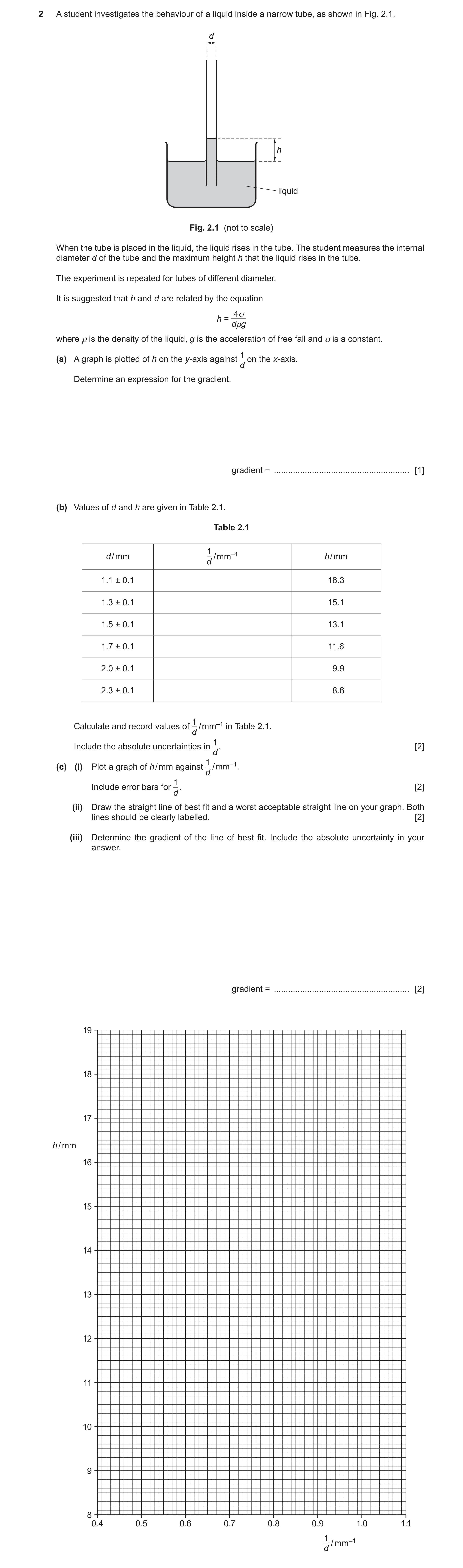
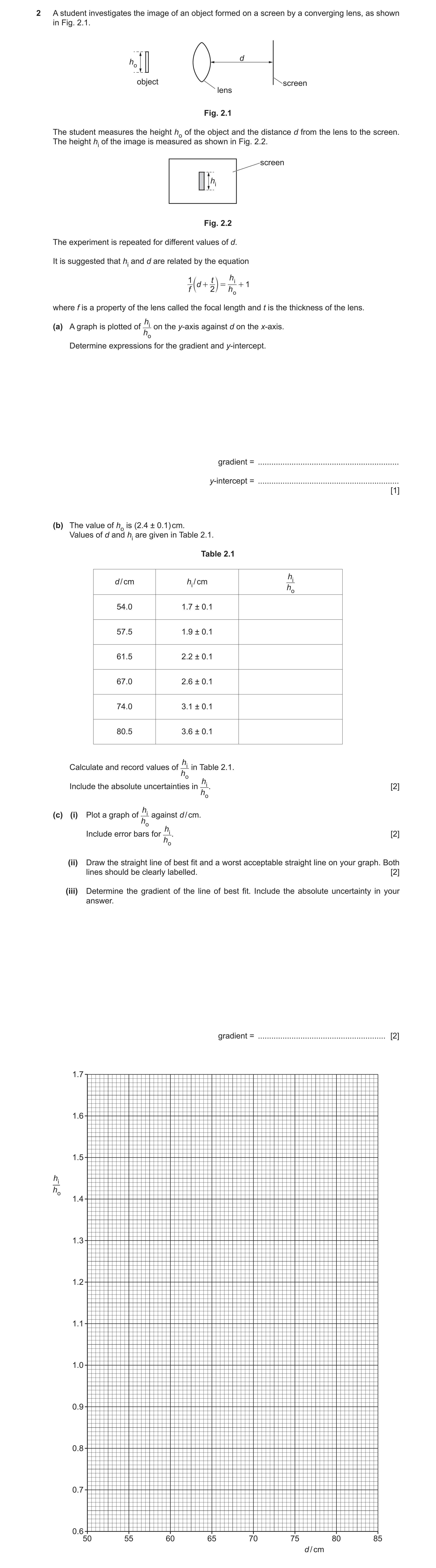
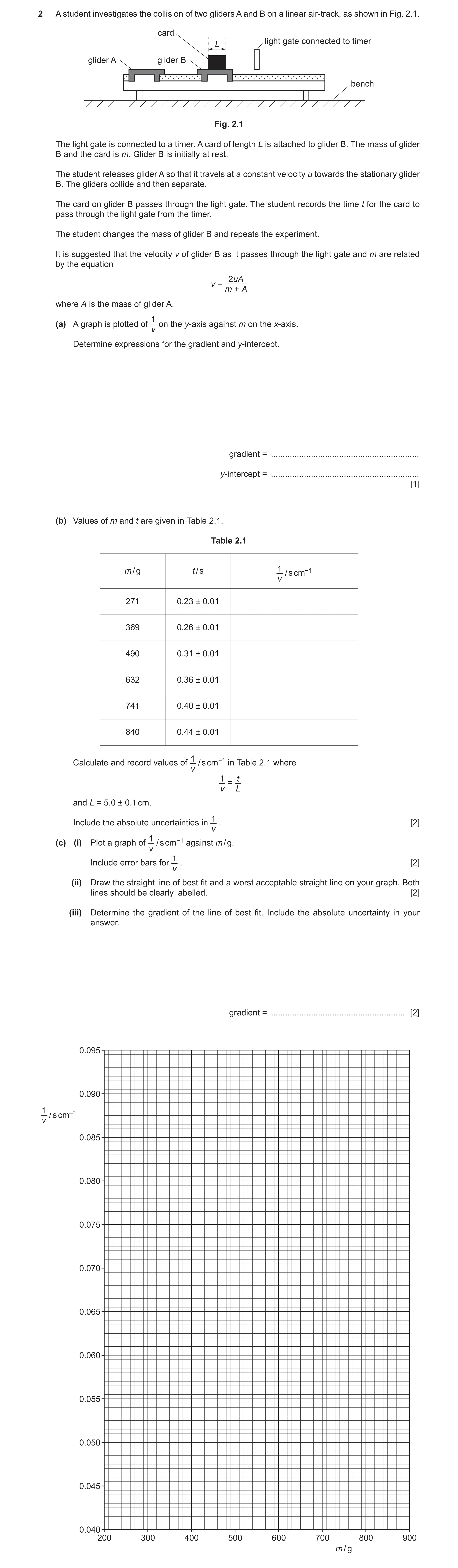
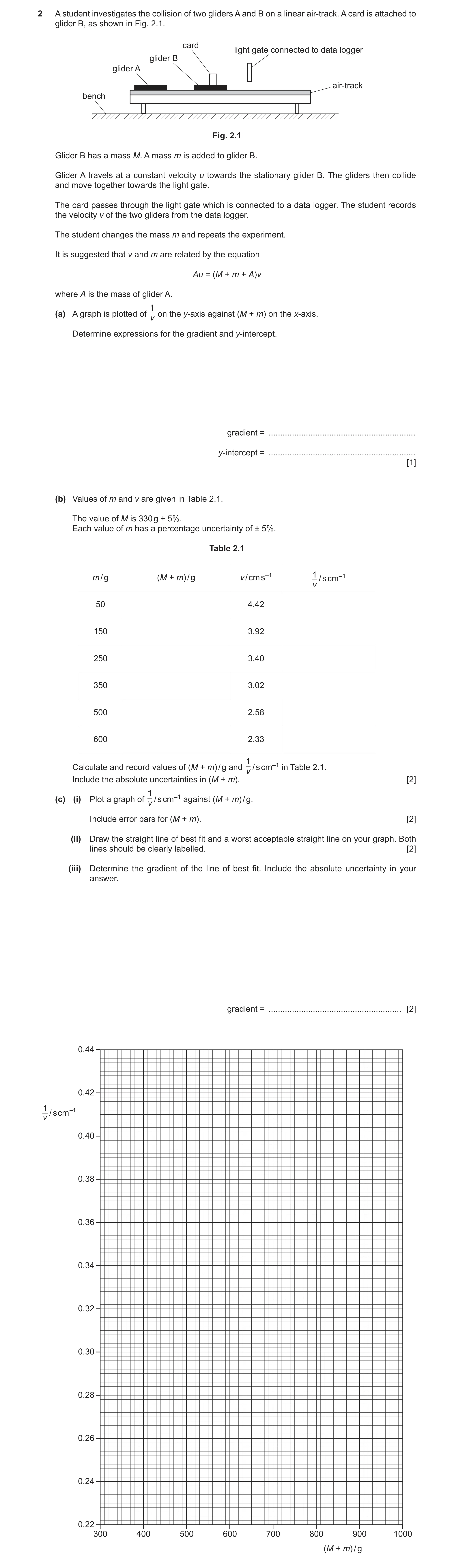
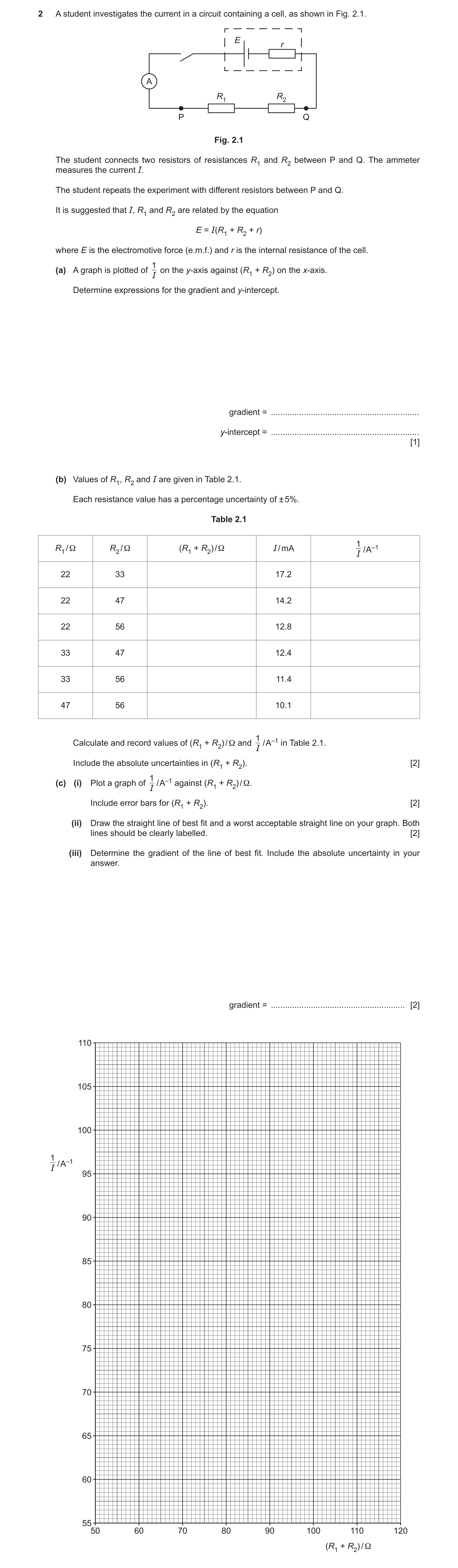
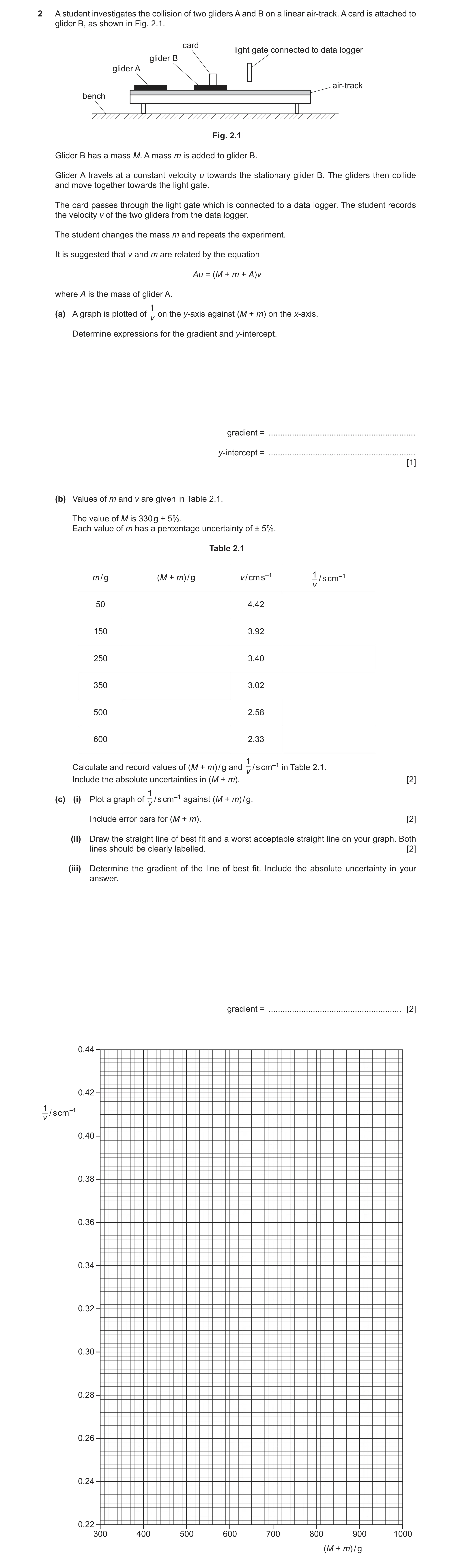
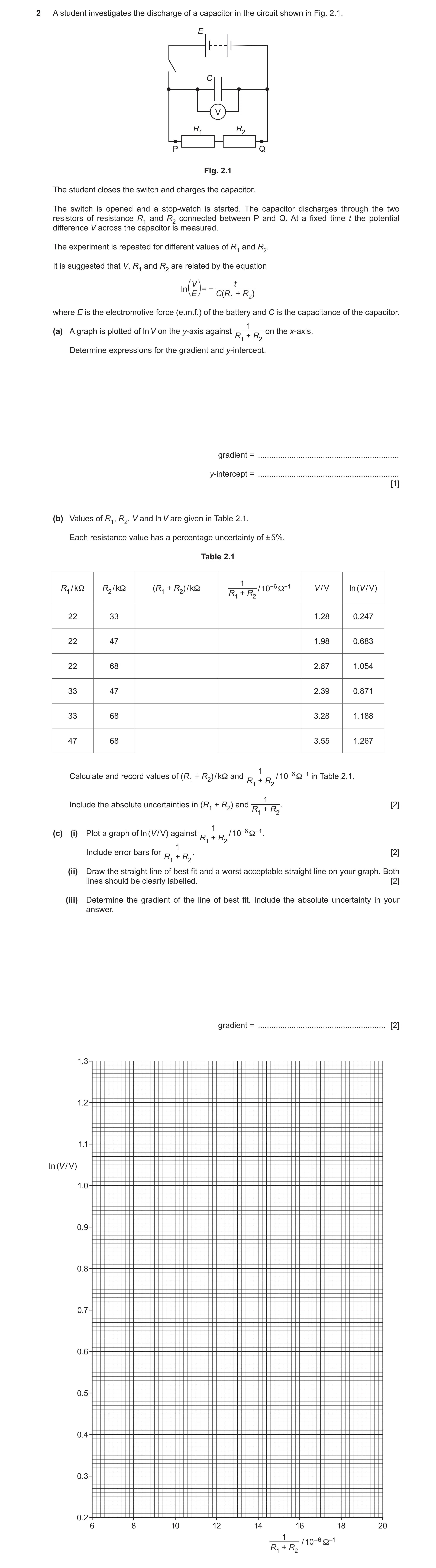
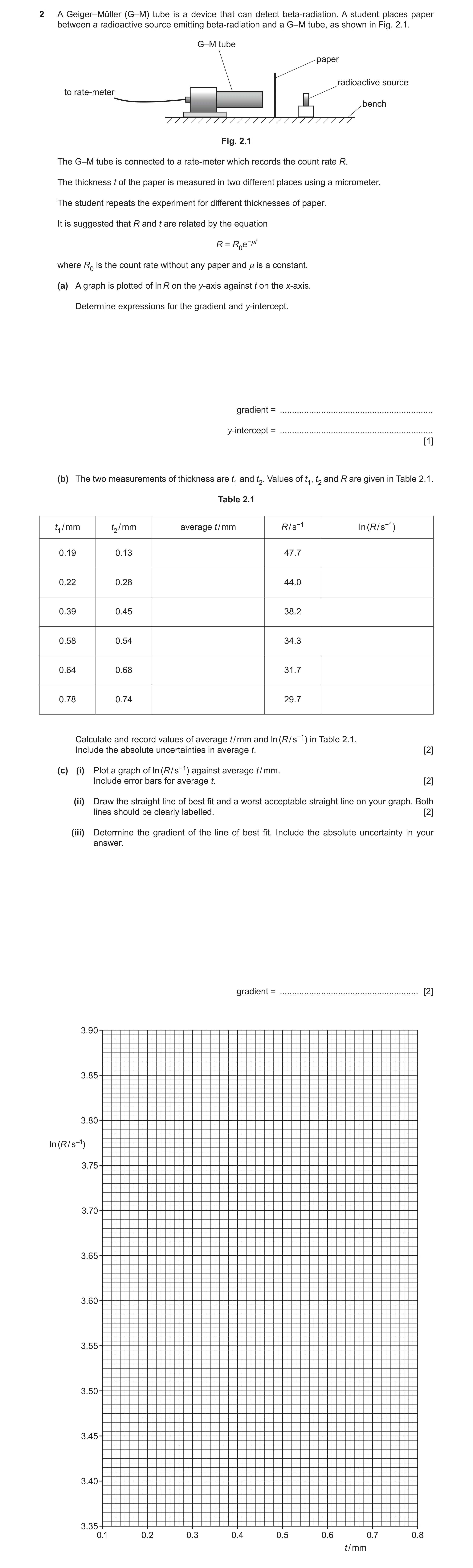
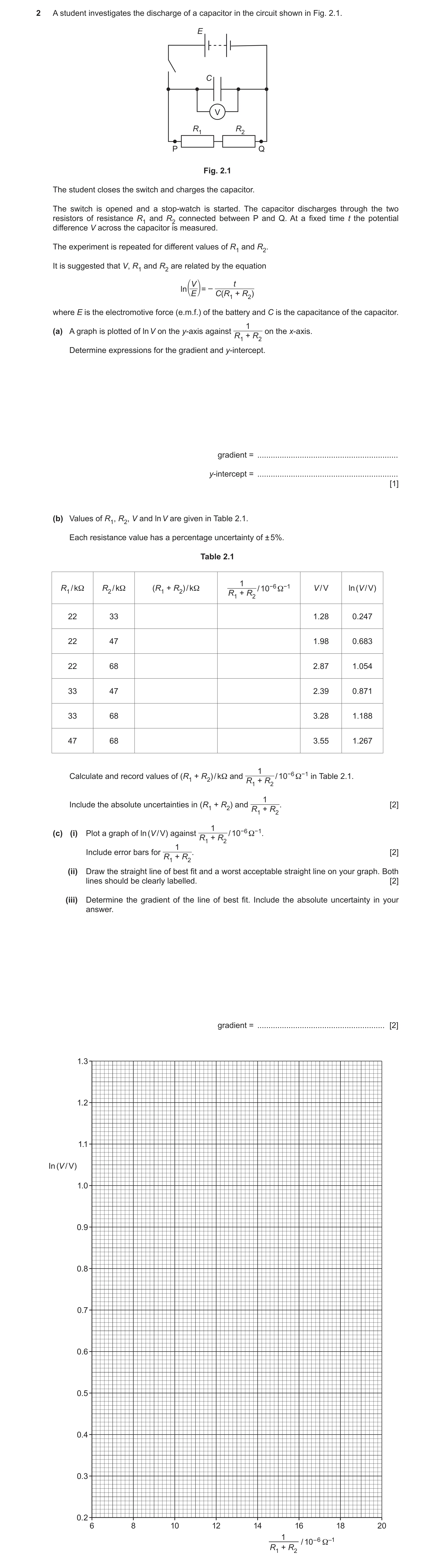
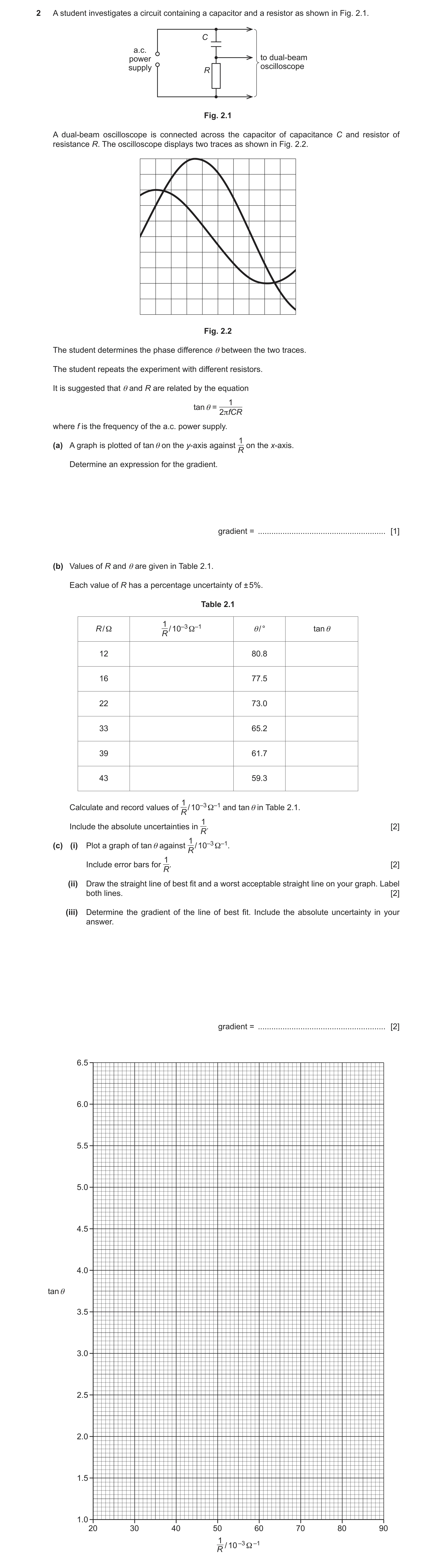
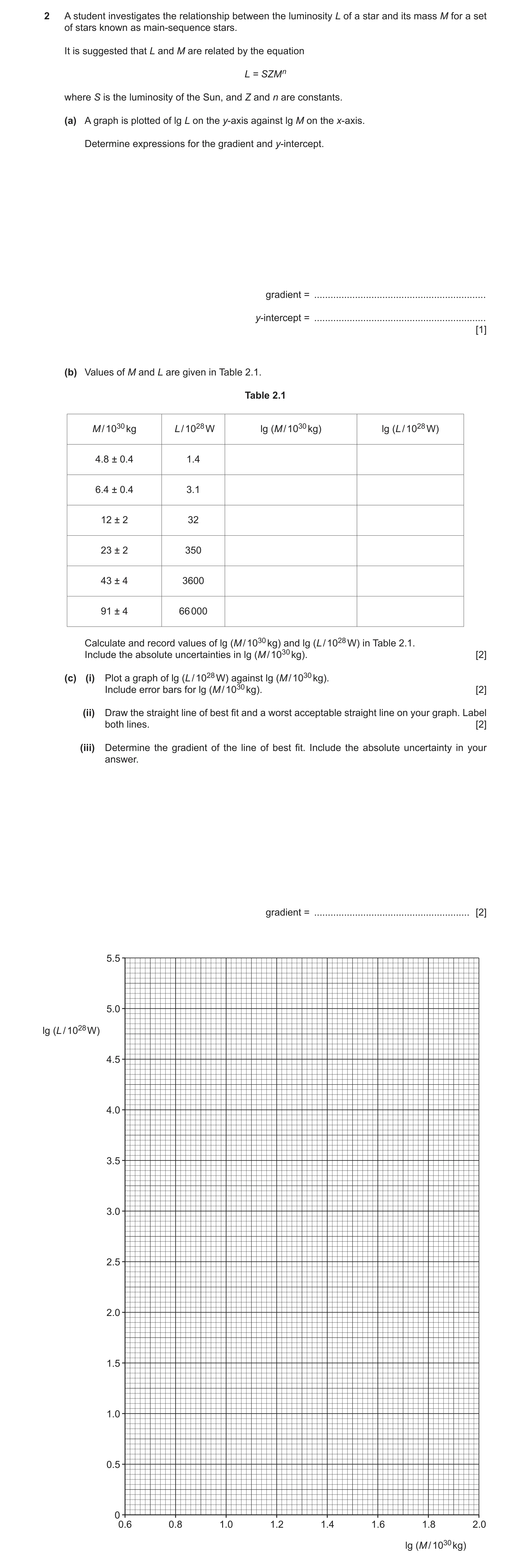
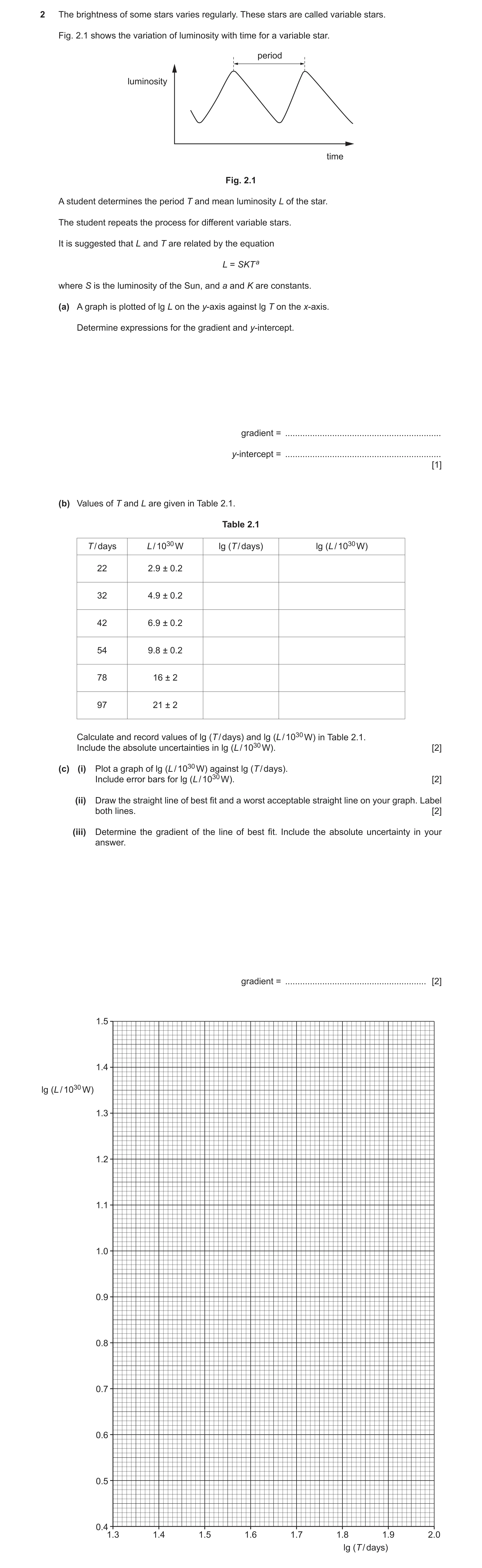
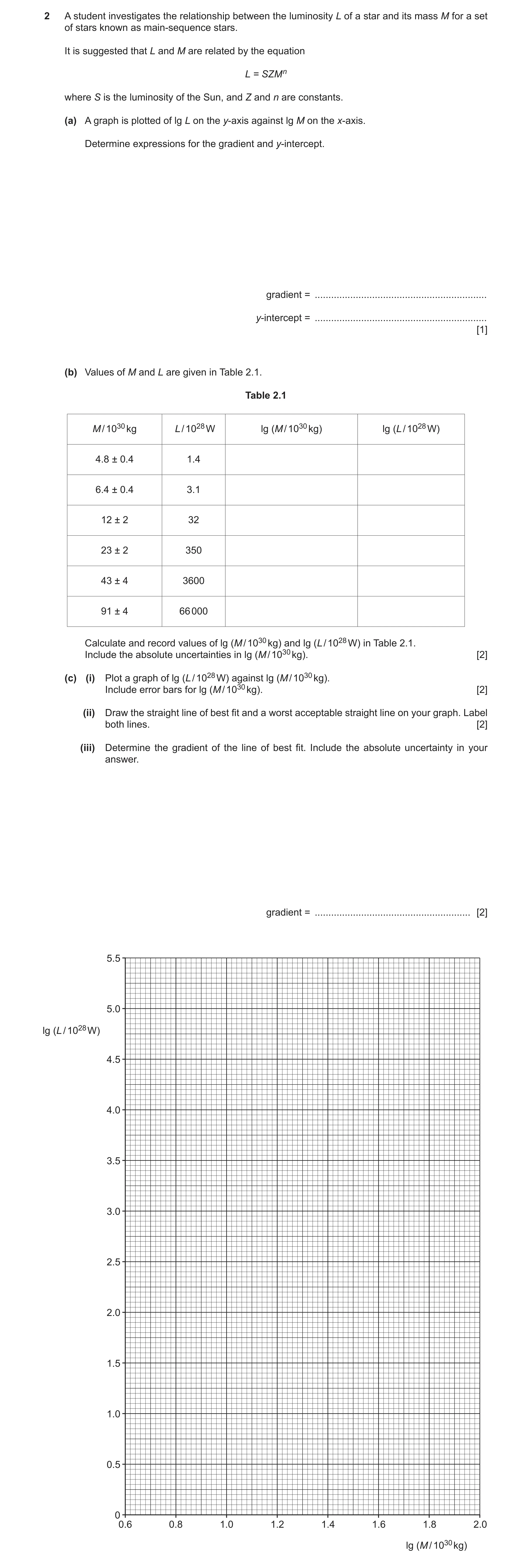
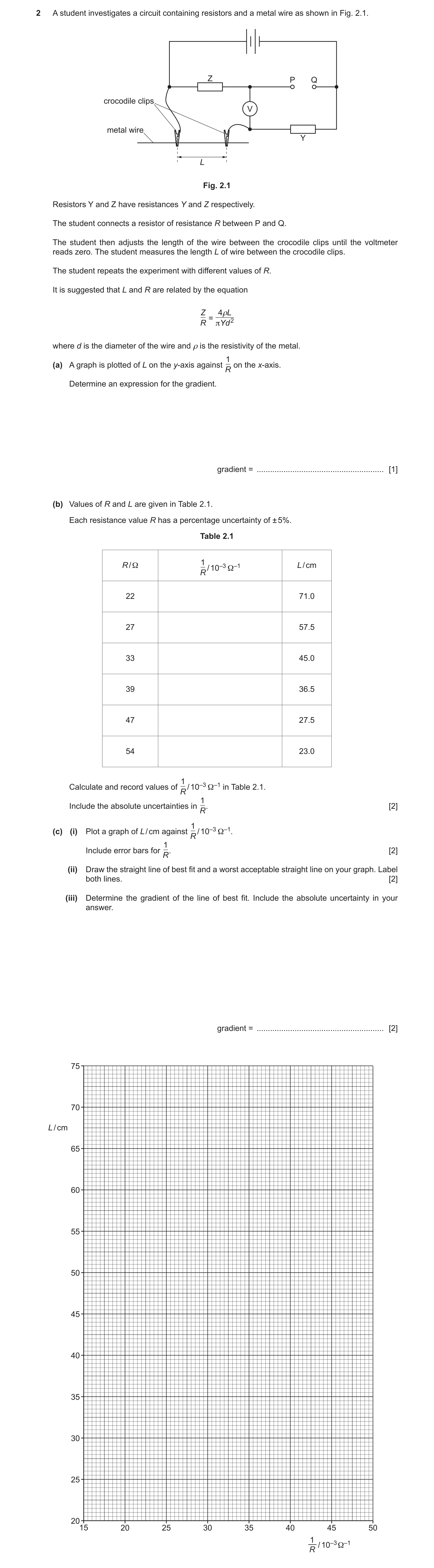
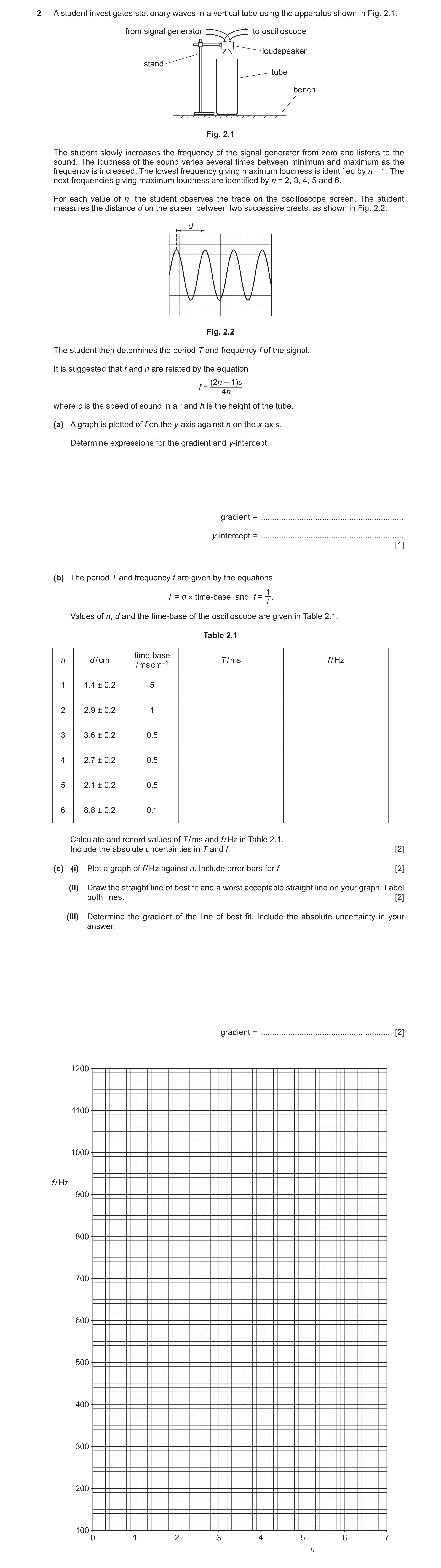
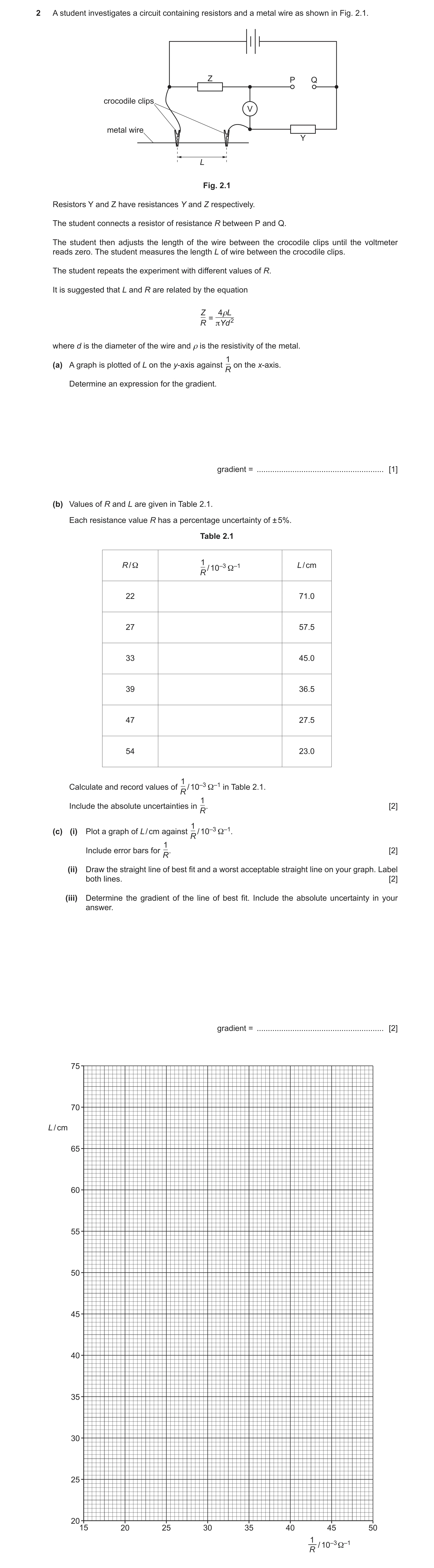
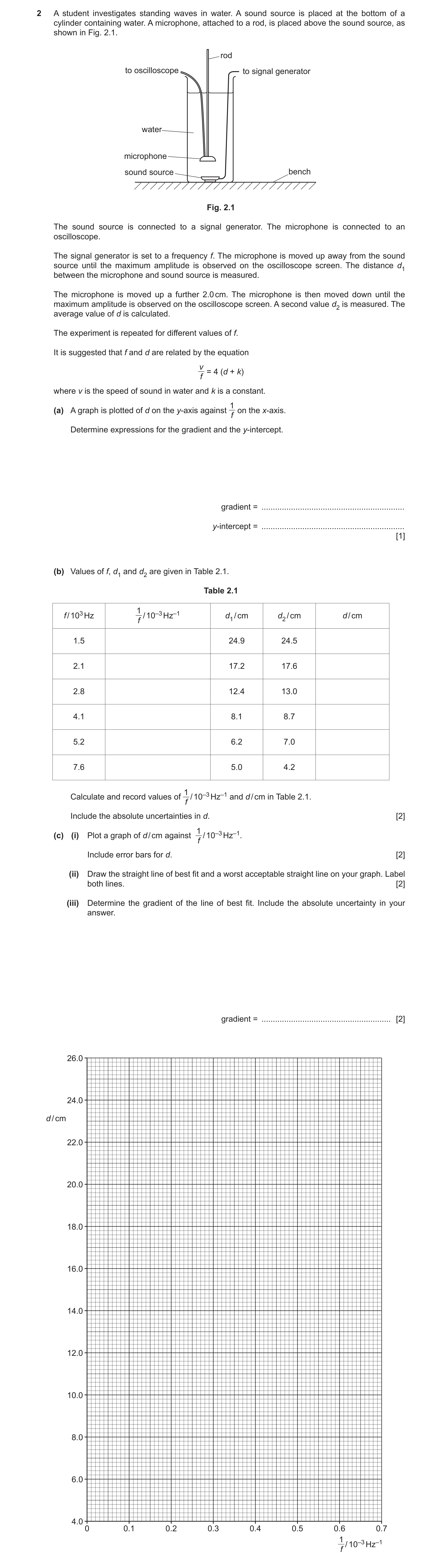
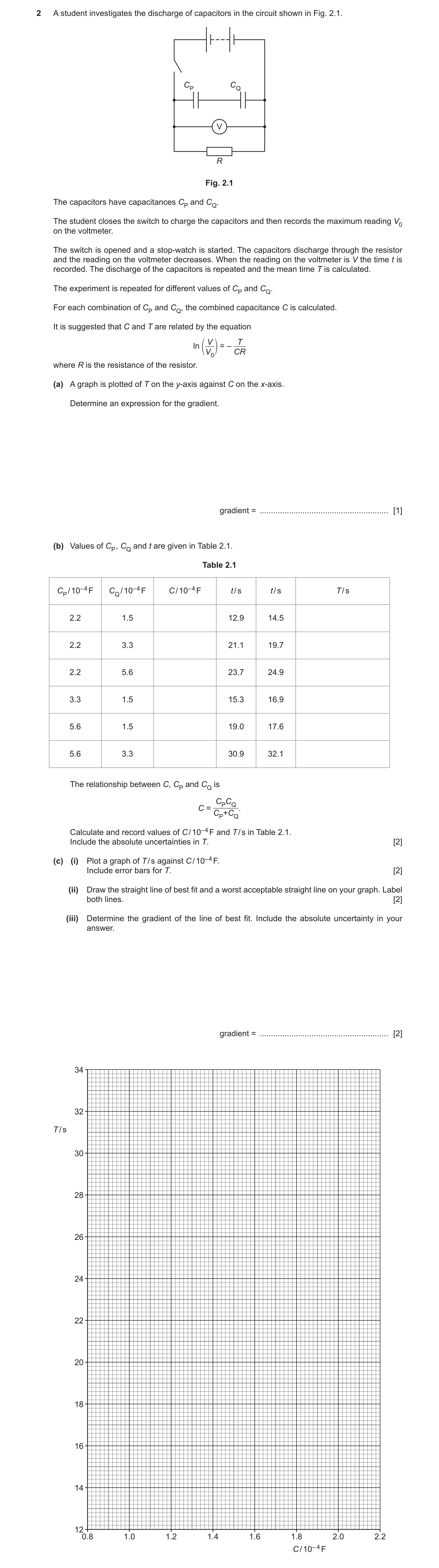
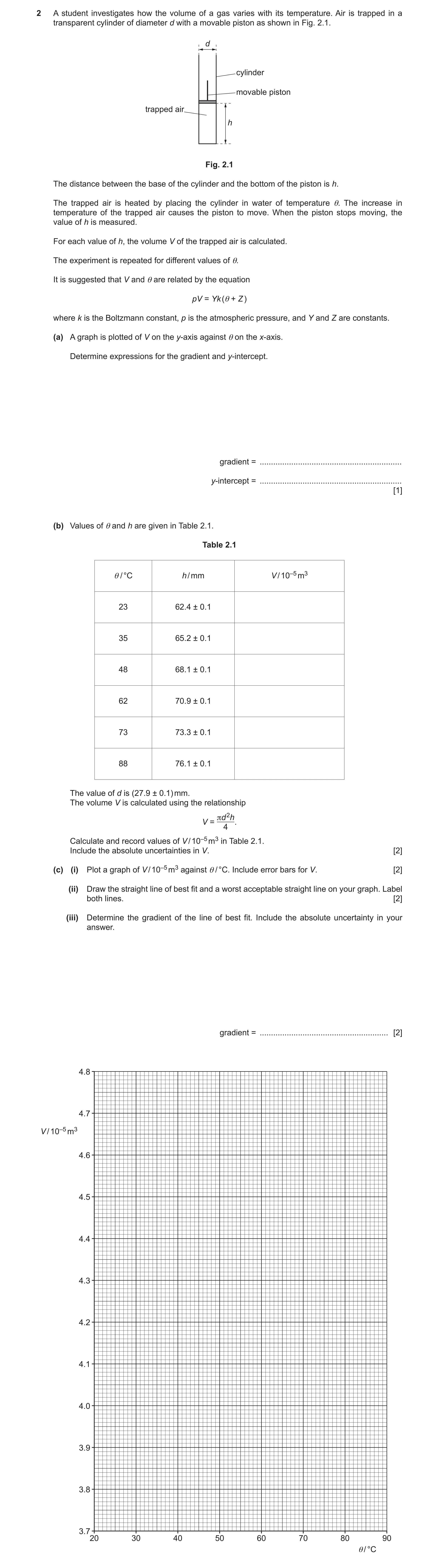
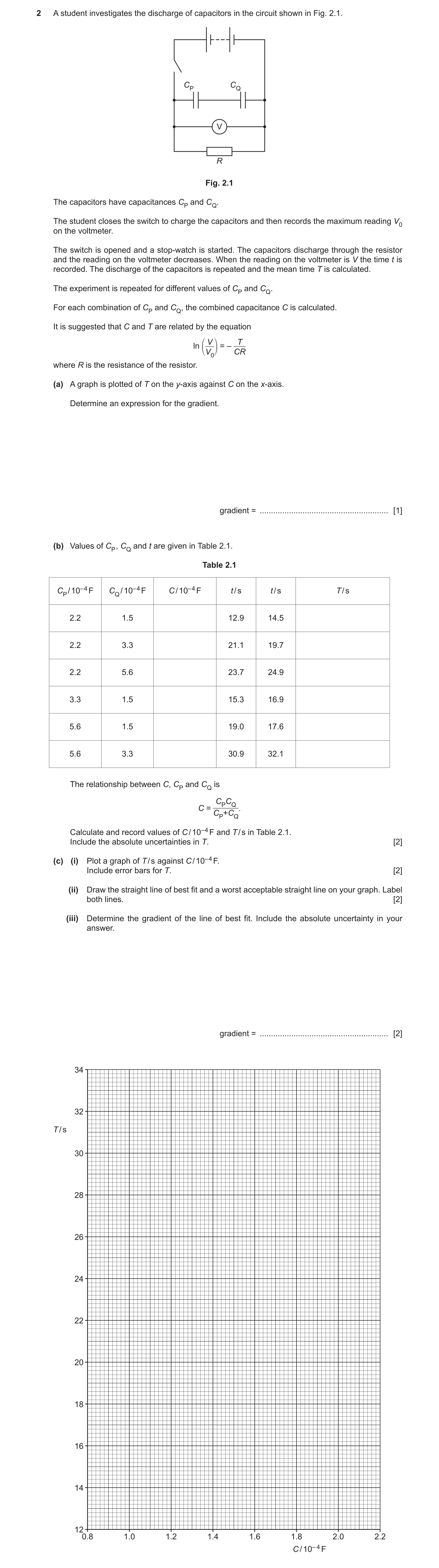
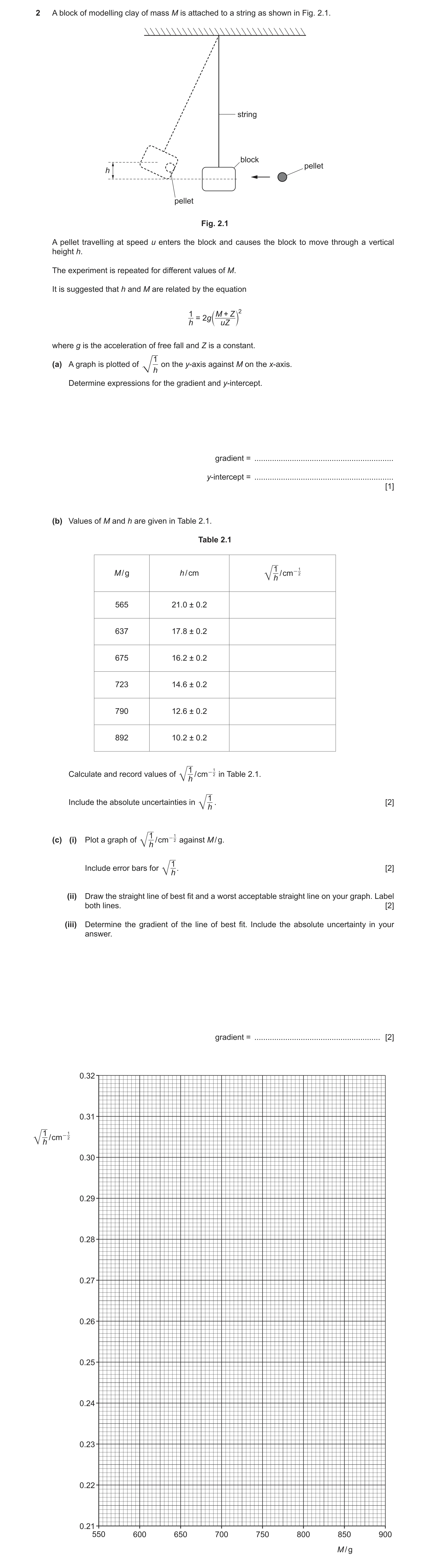
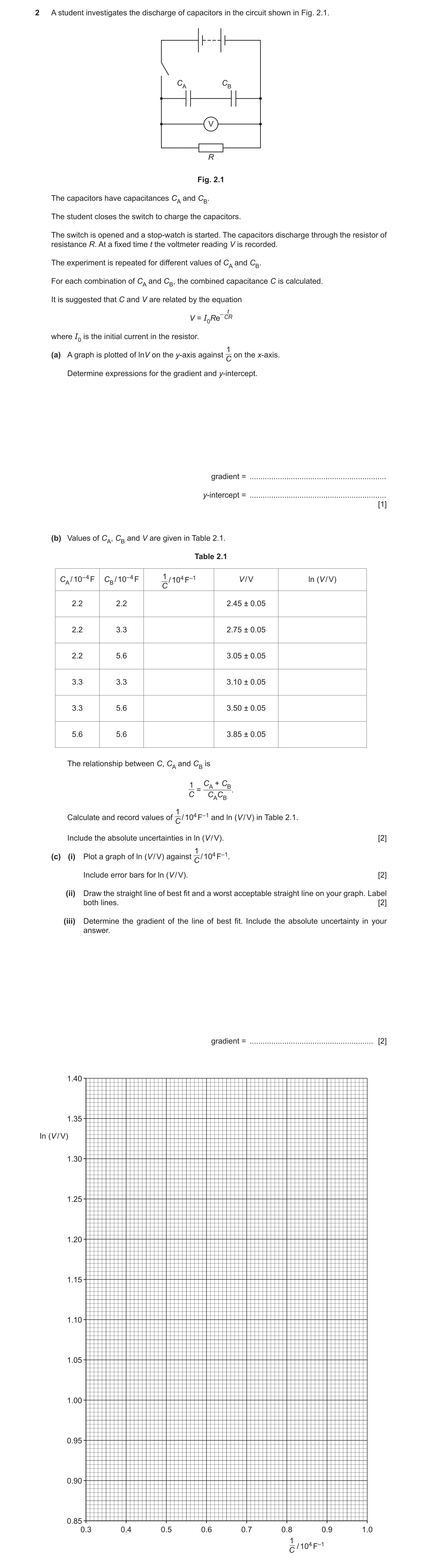
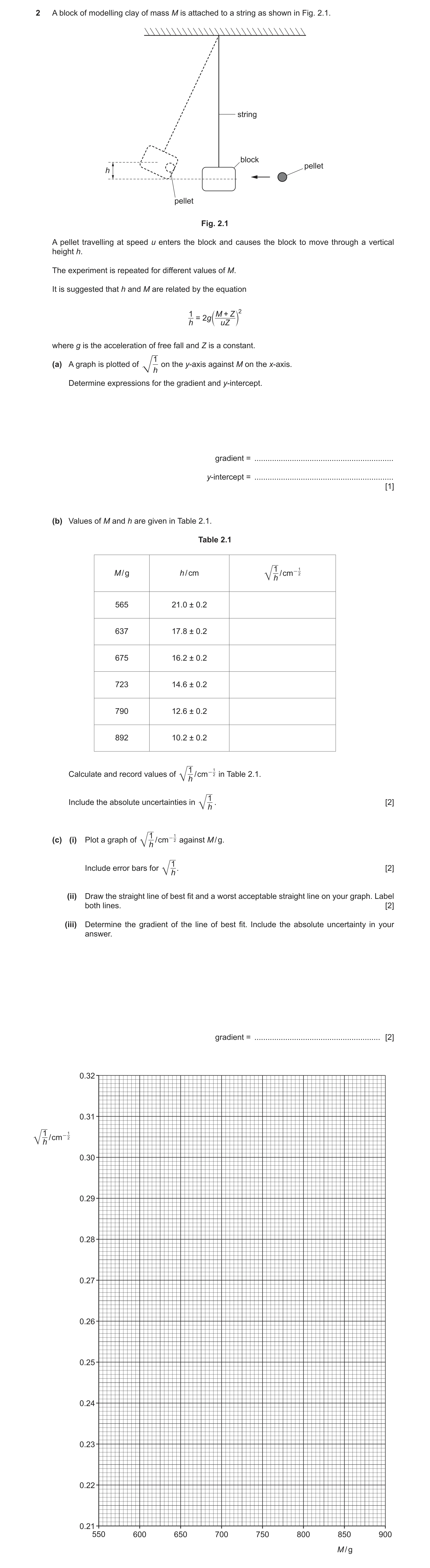
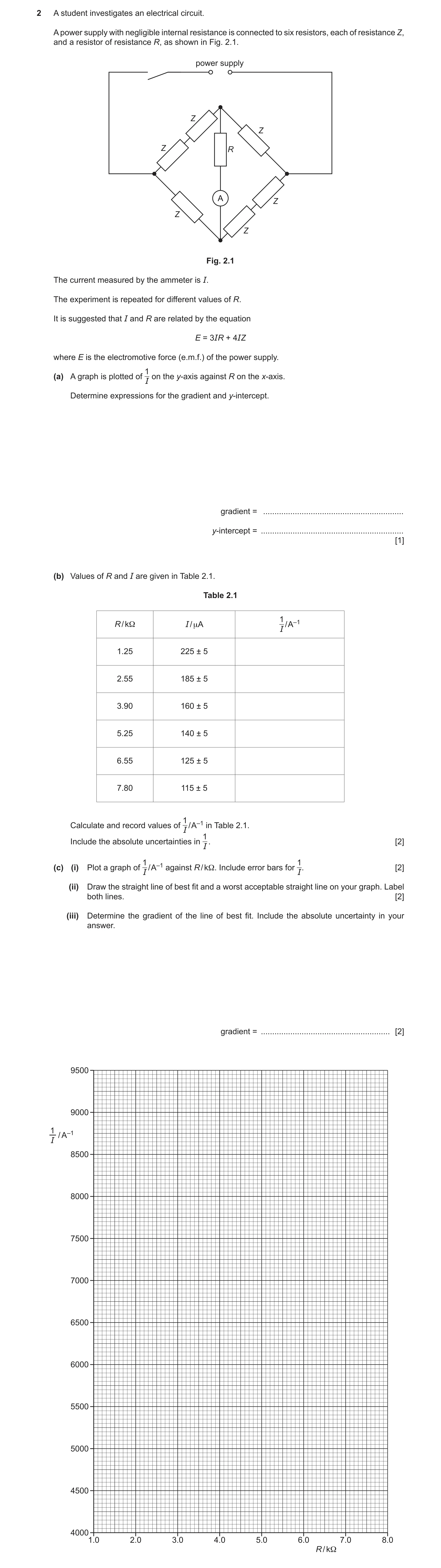
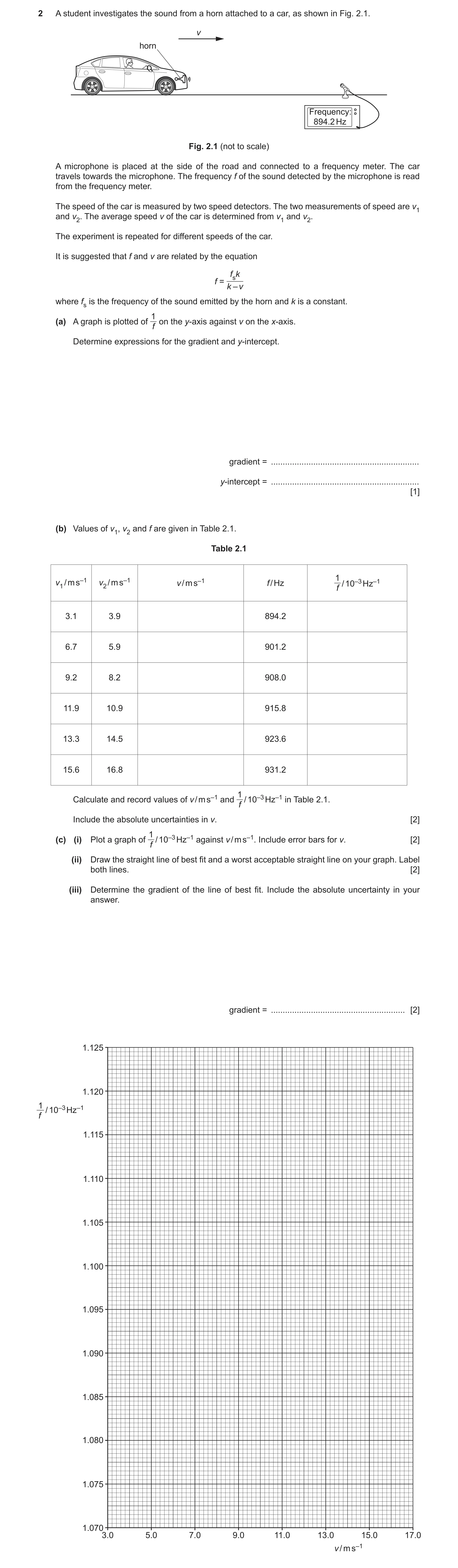
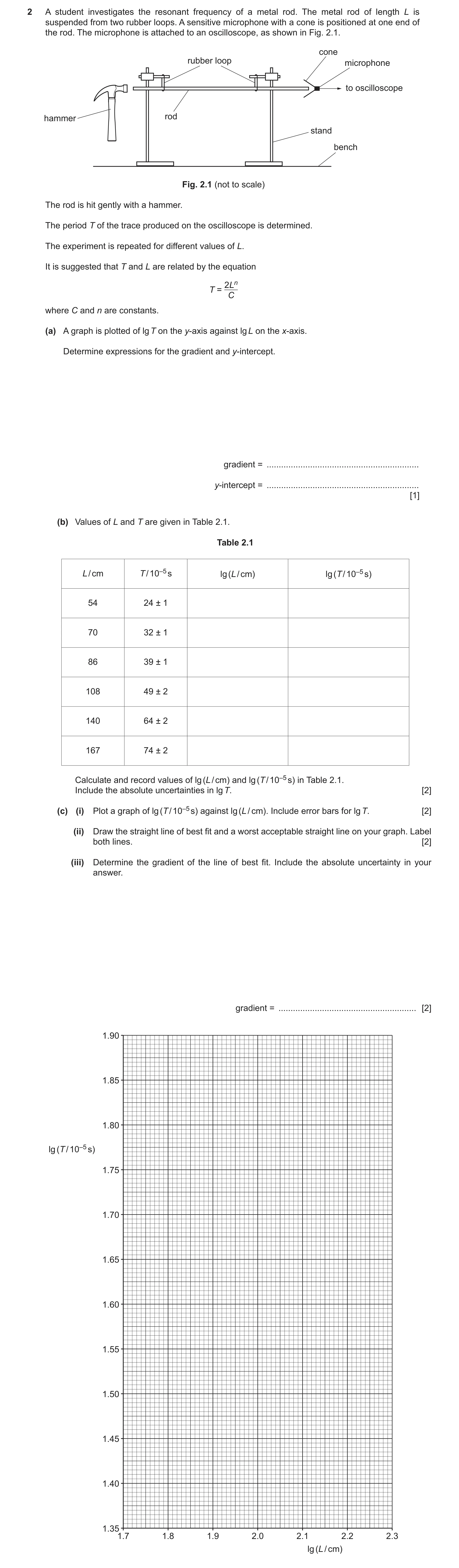
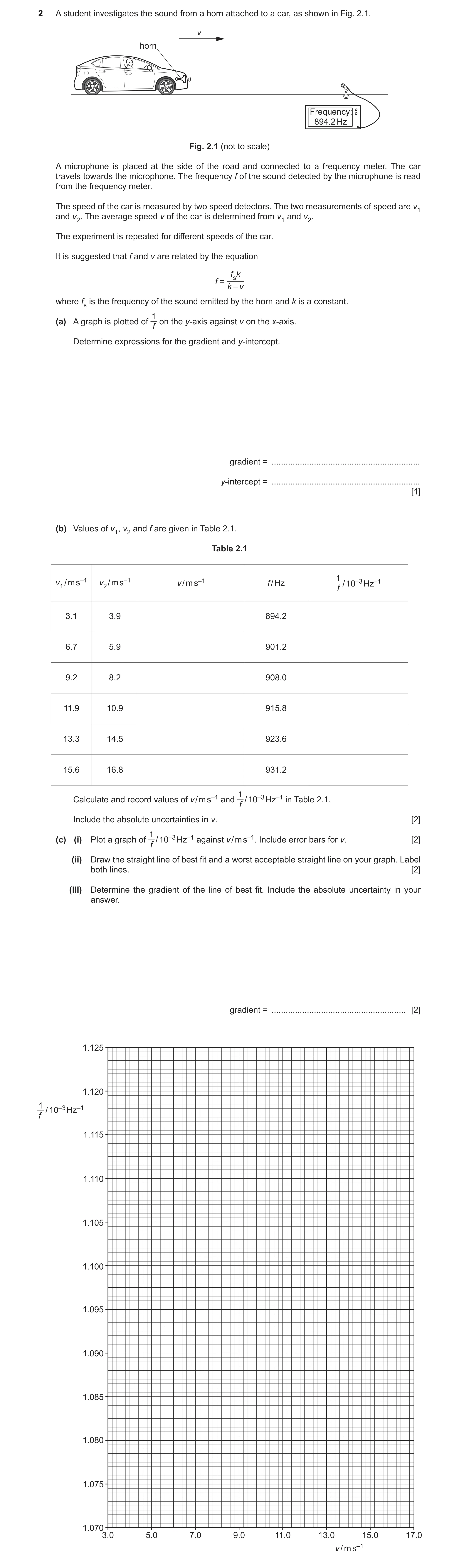
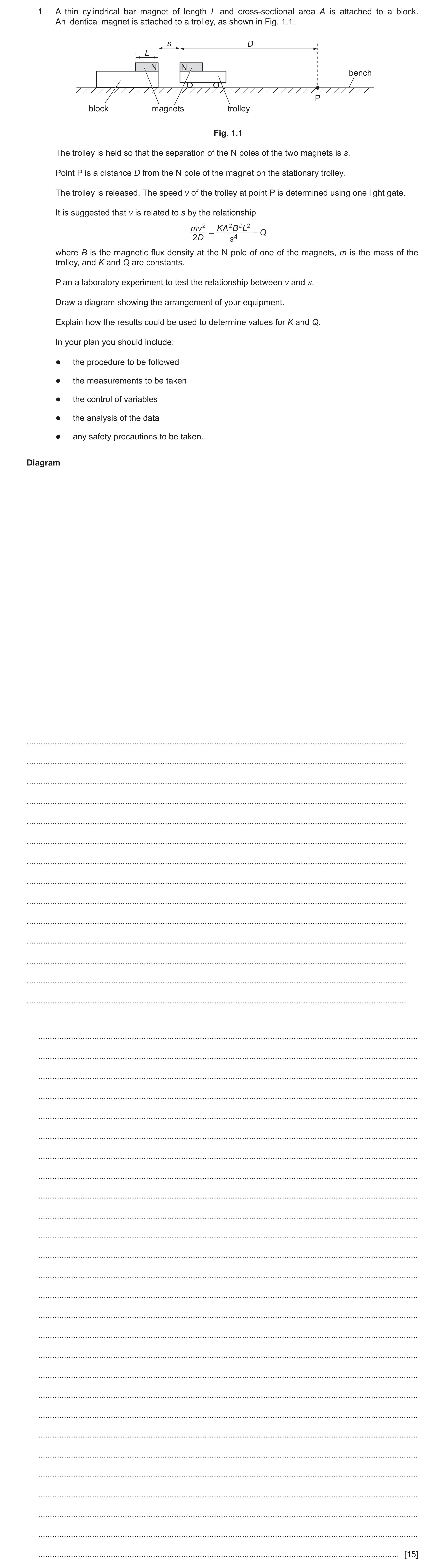
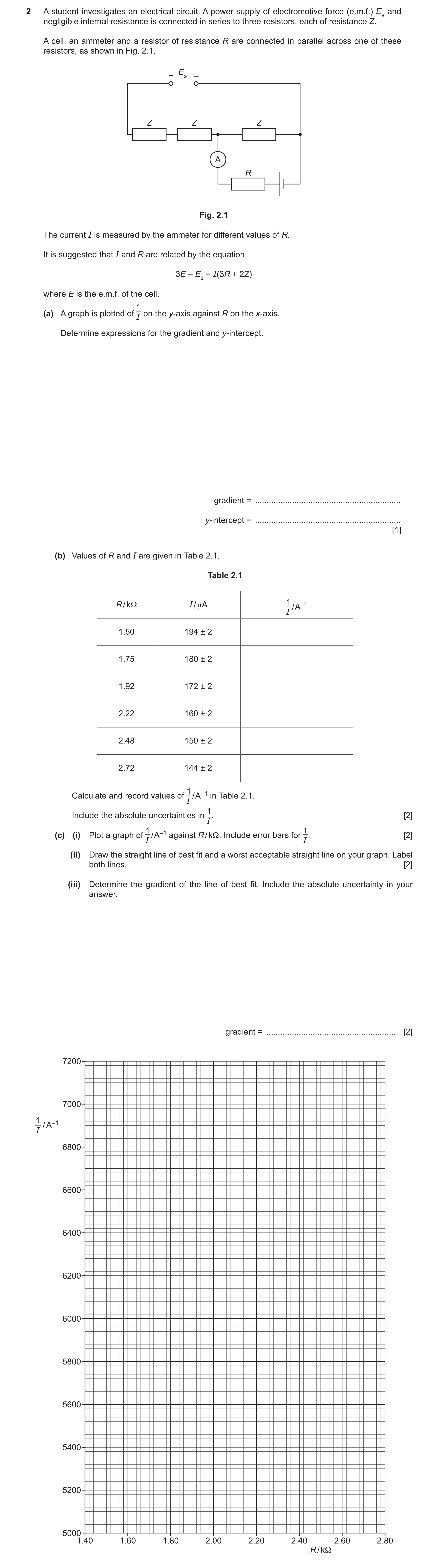
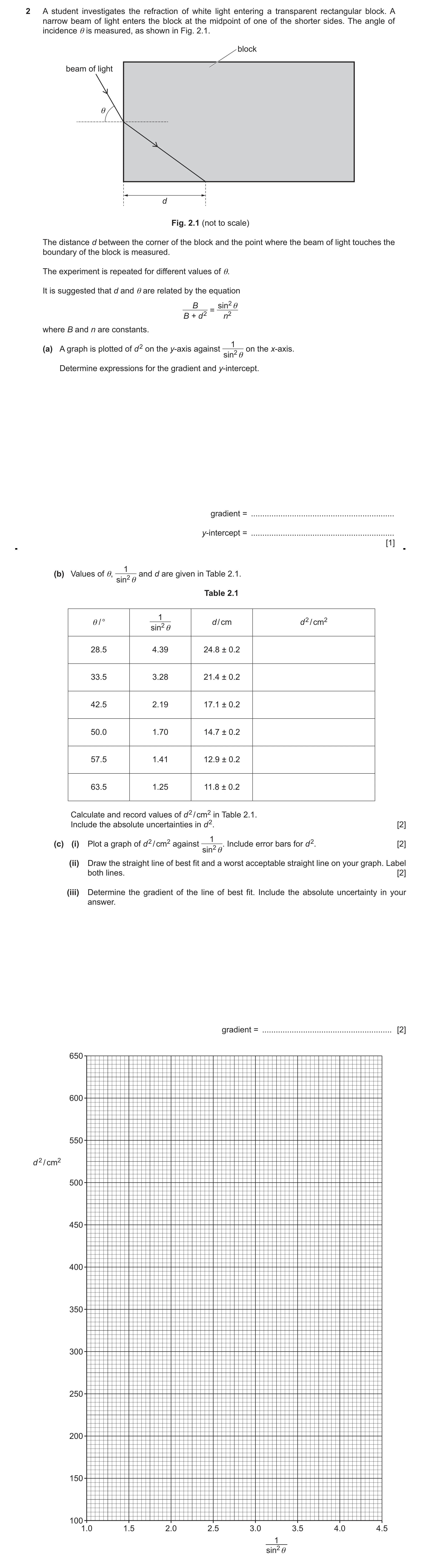
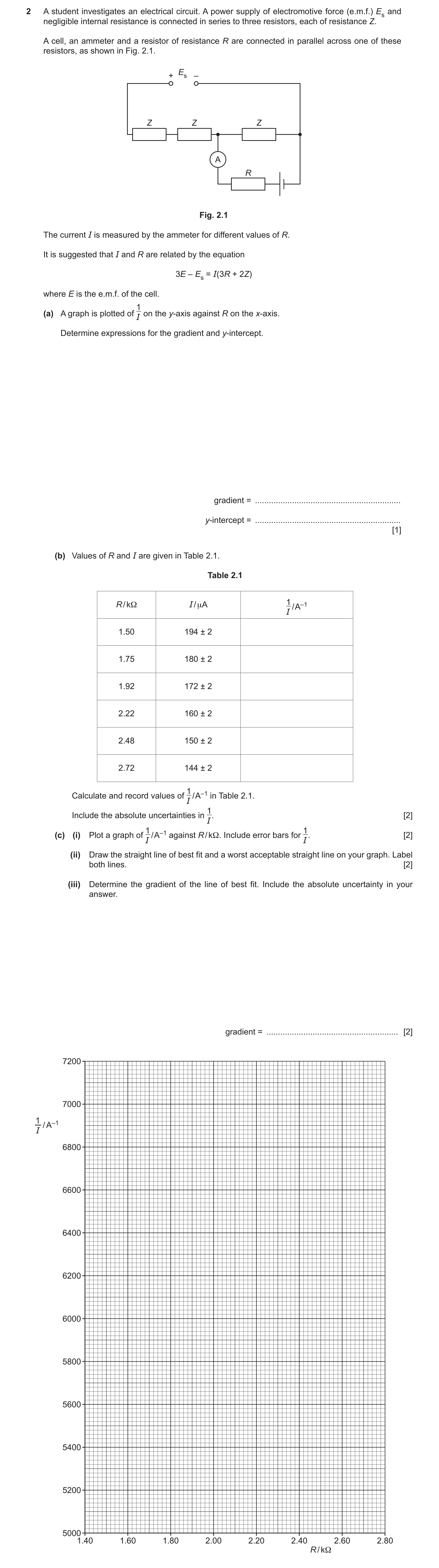
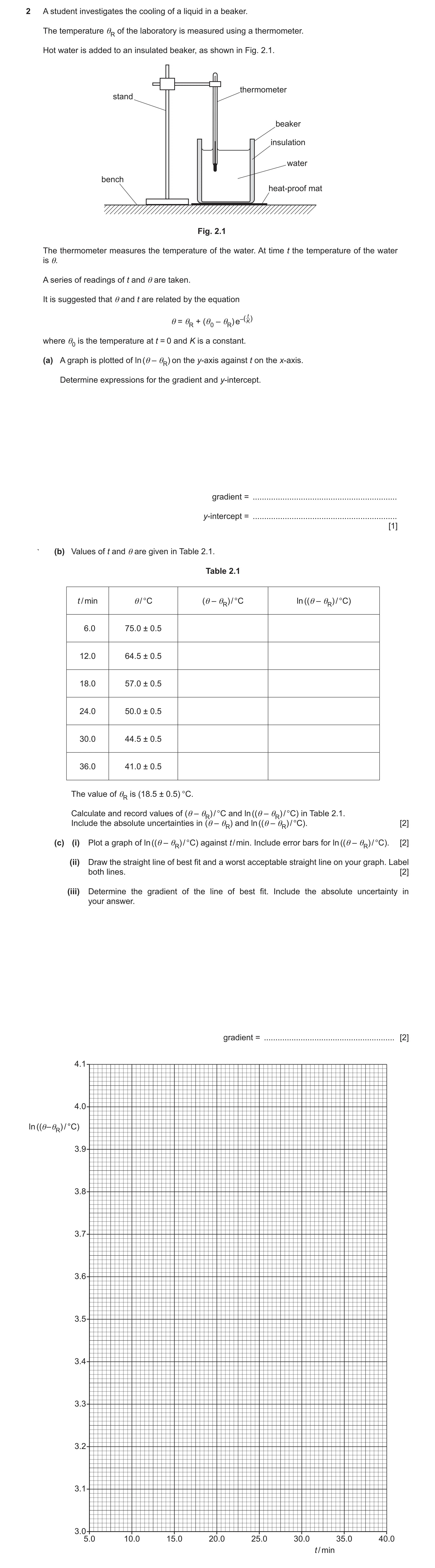
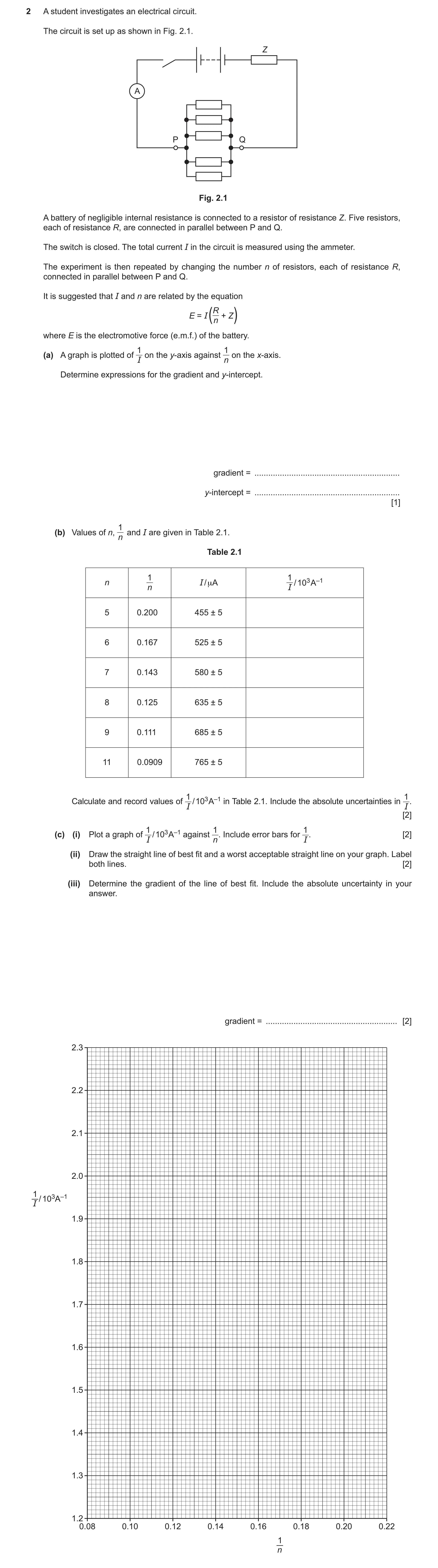
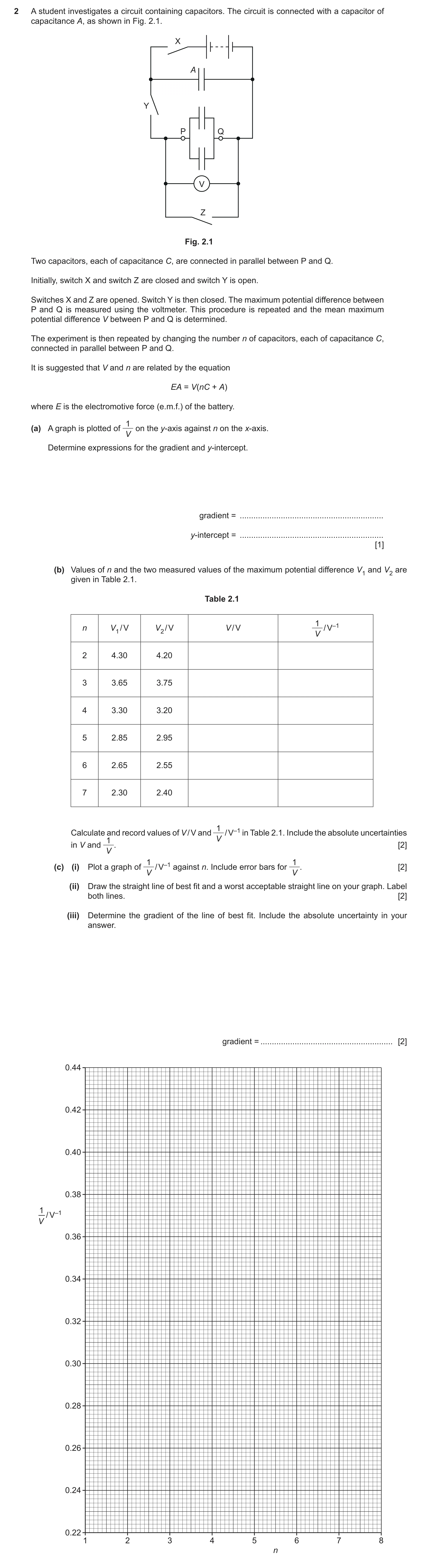
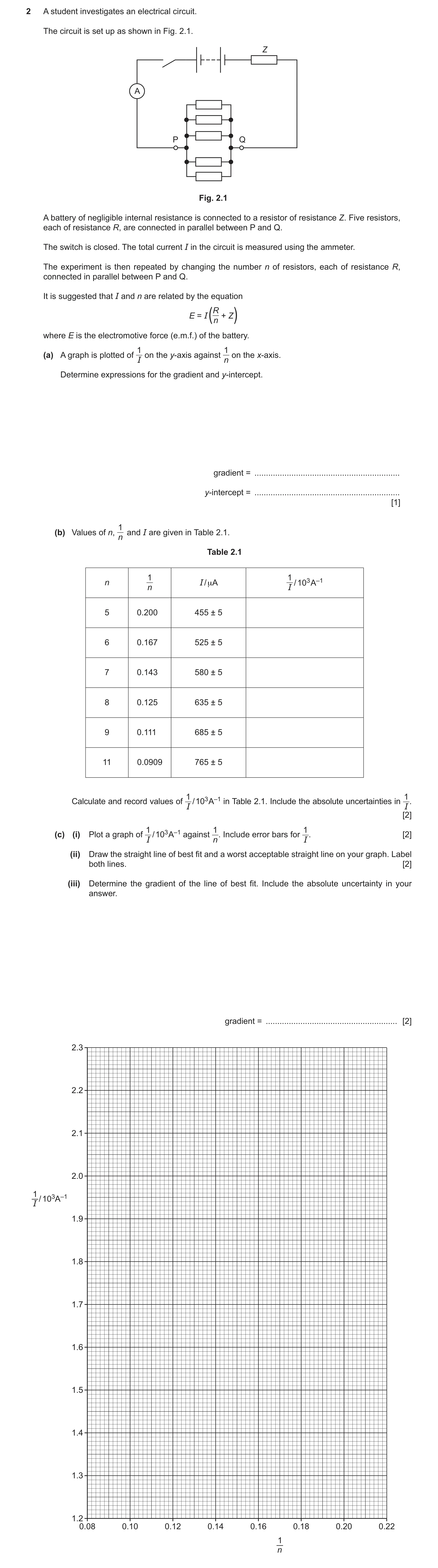
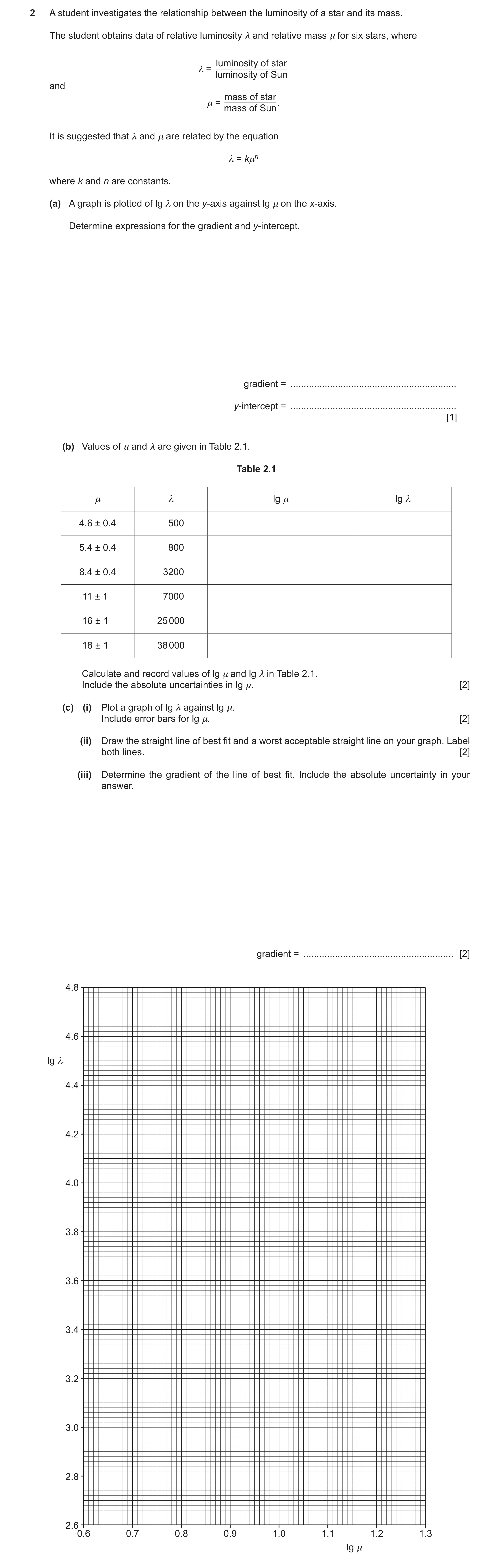
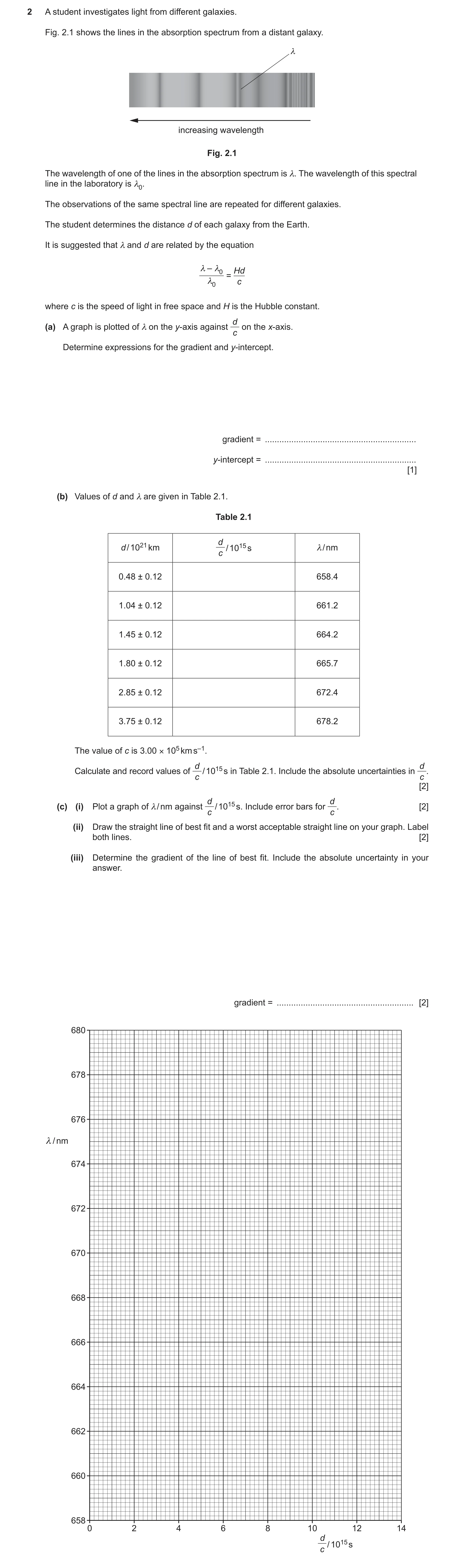
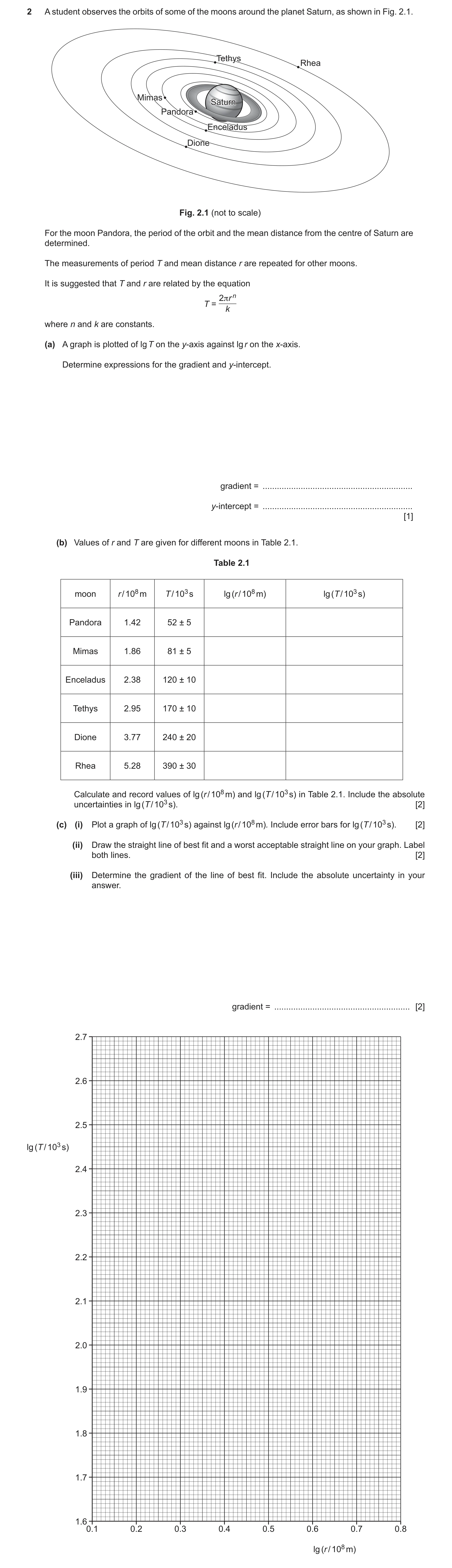
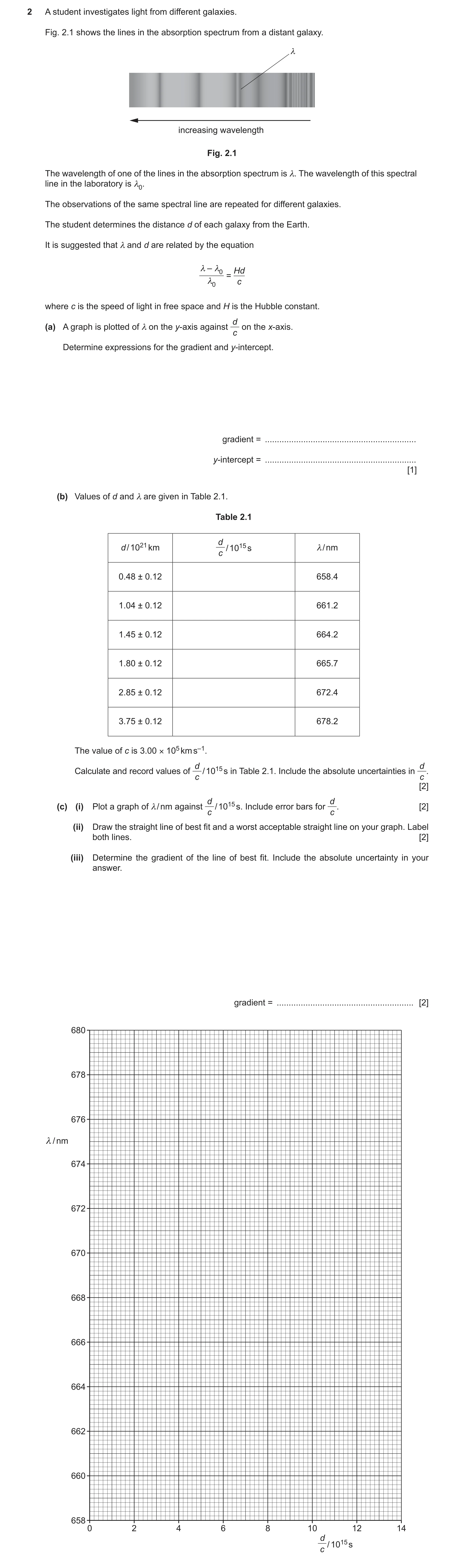
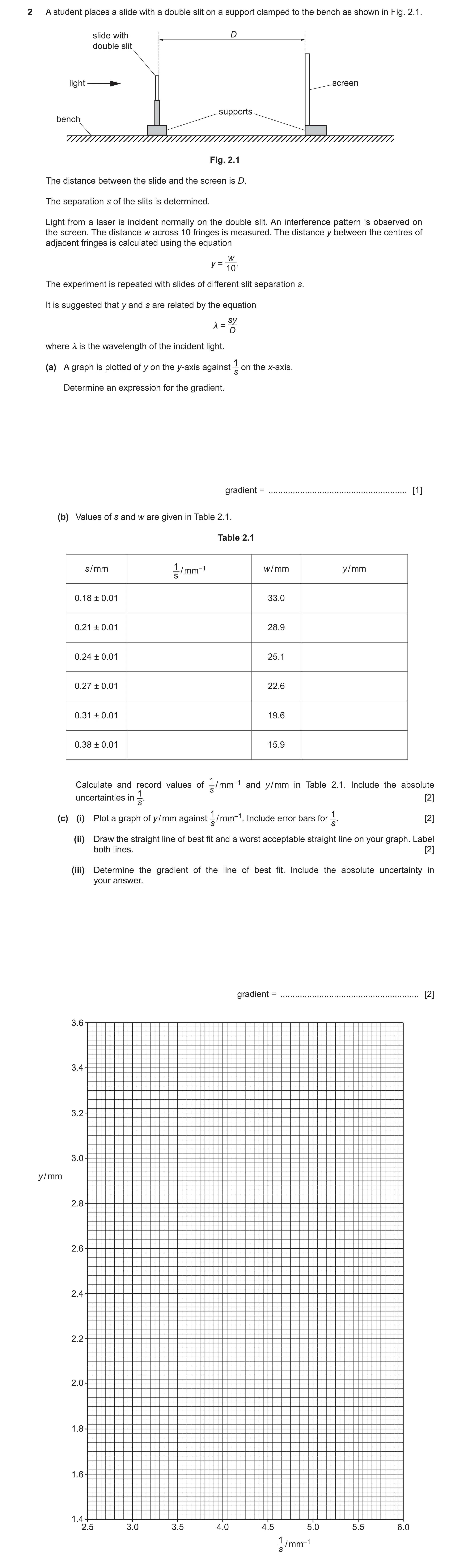
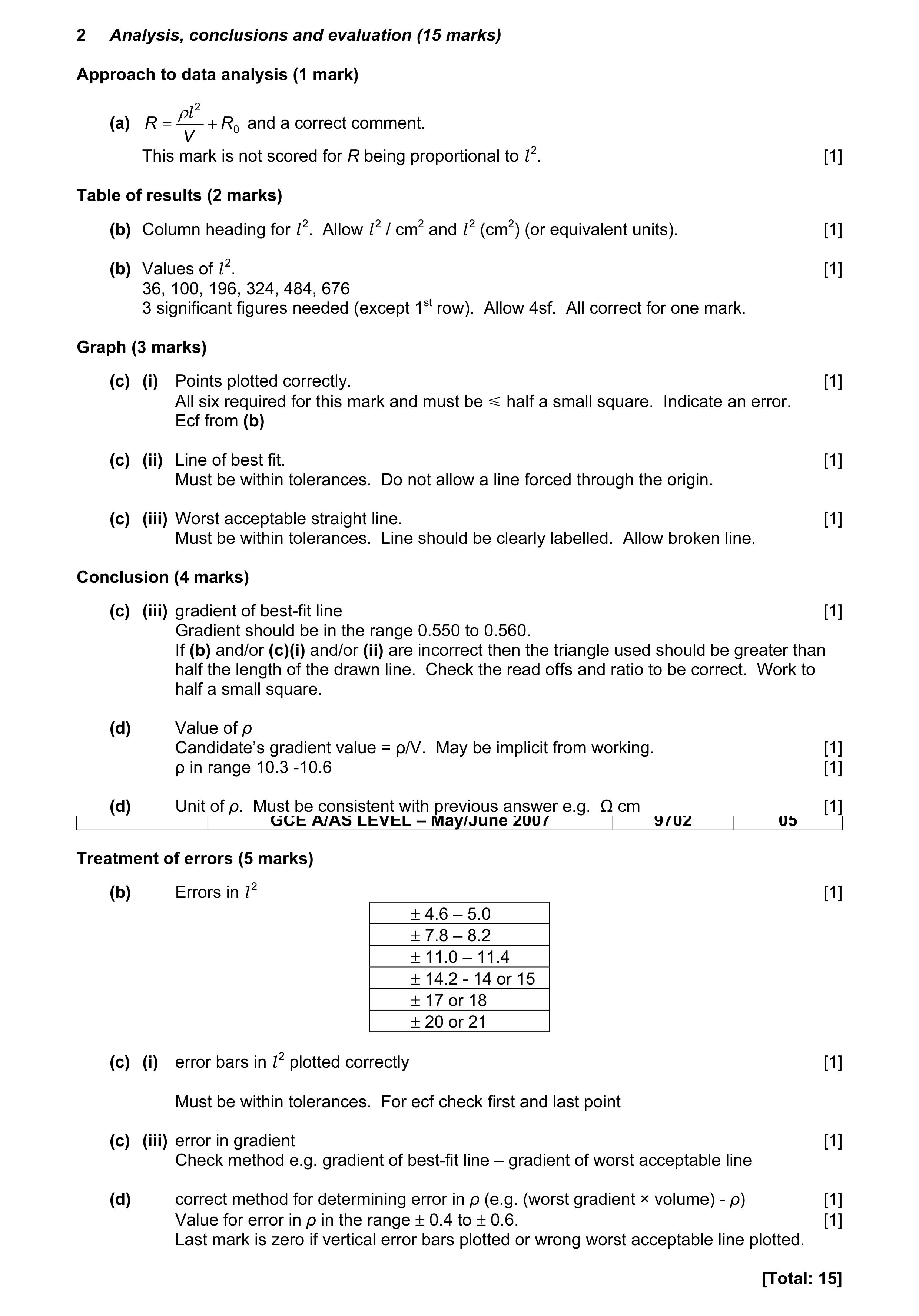 10
10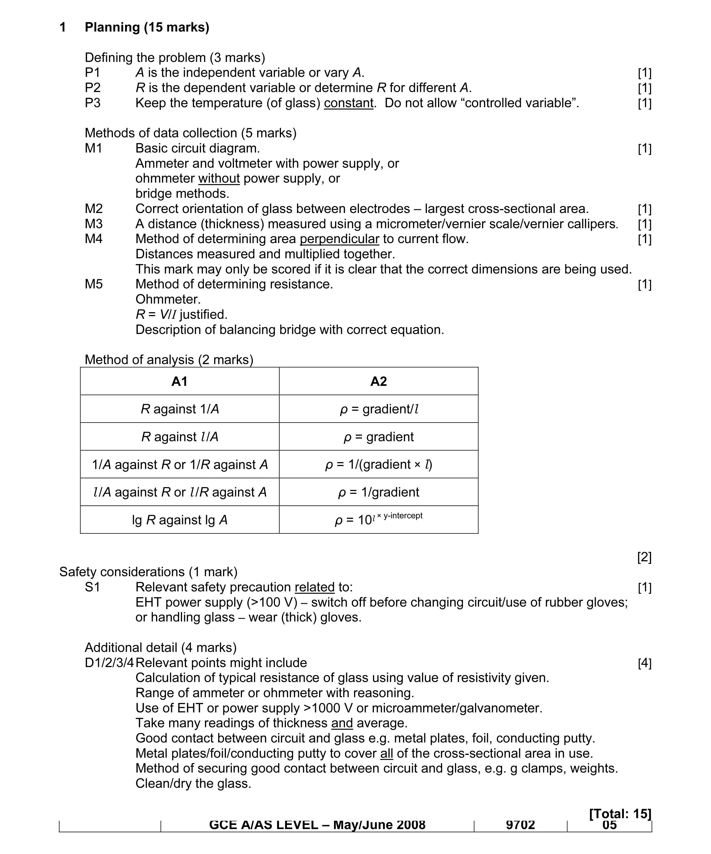 15
15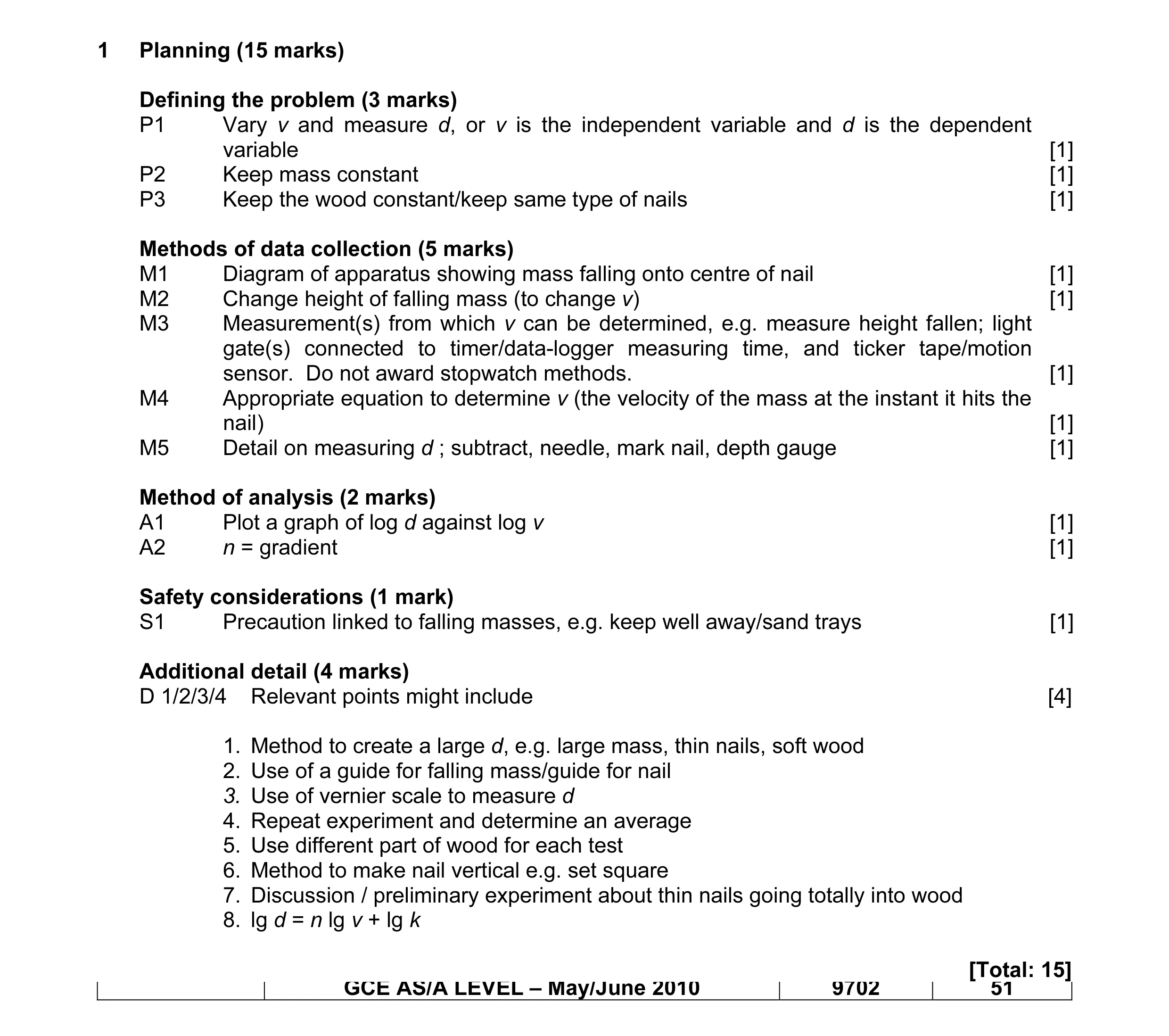 15
15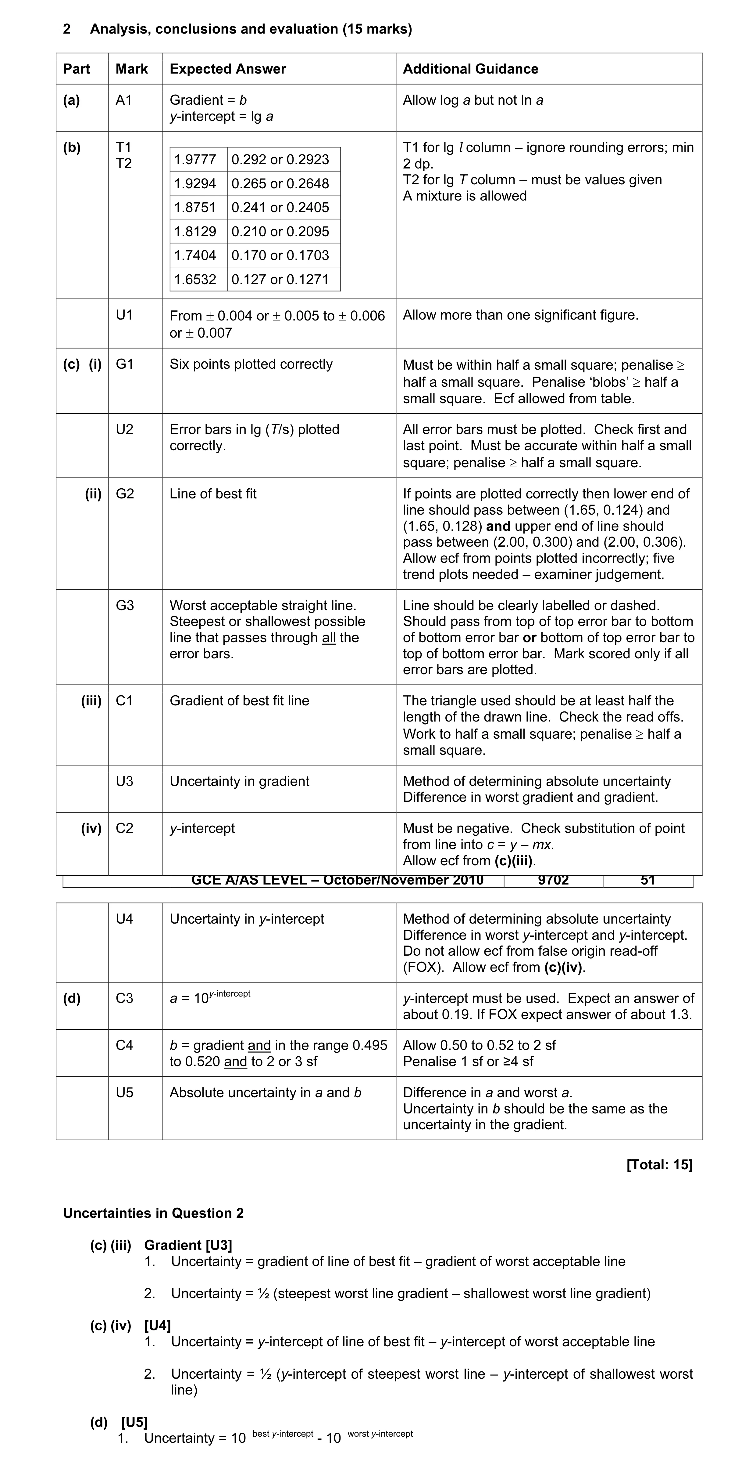 10
10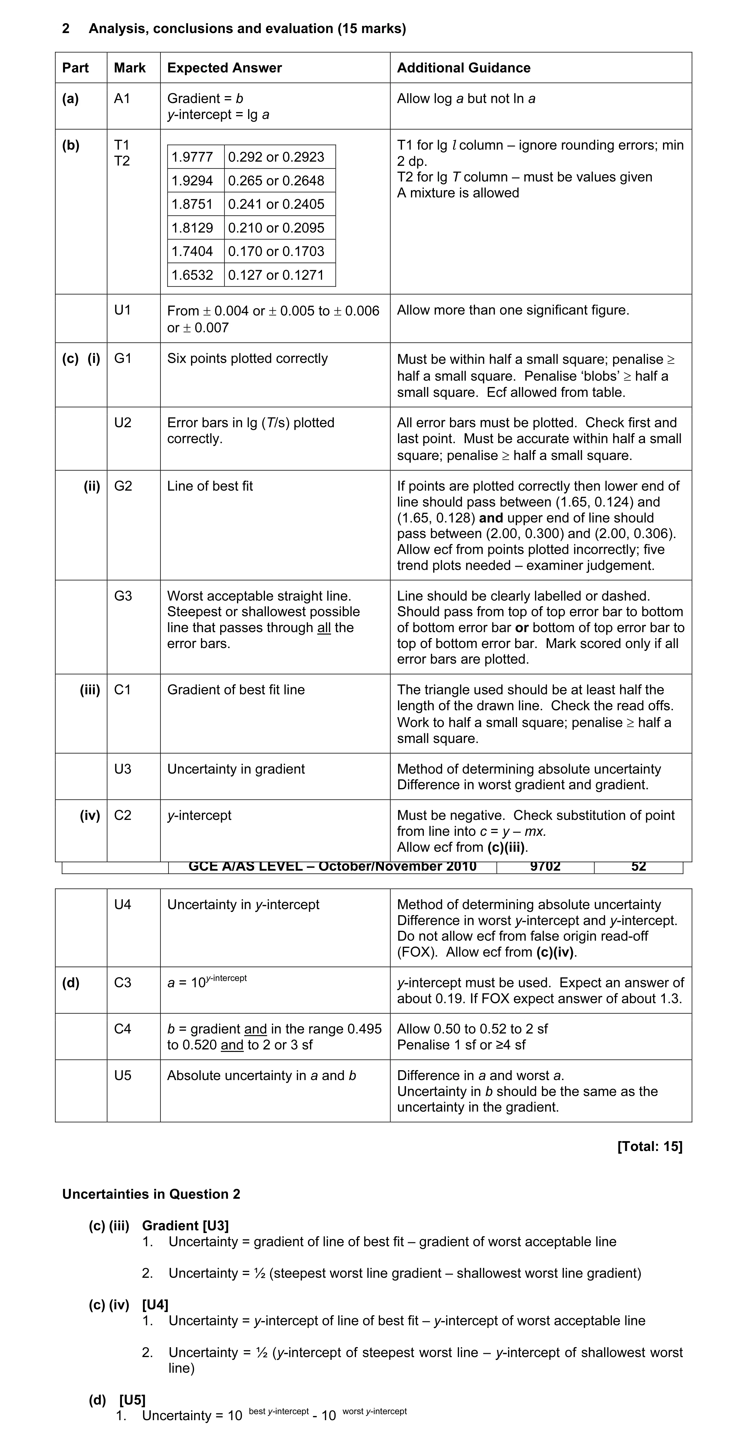 10
10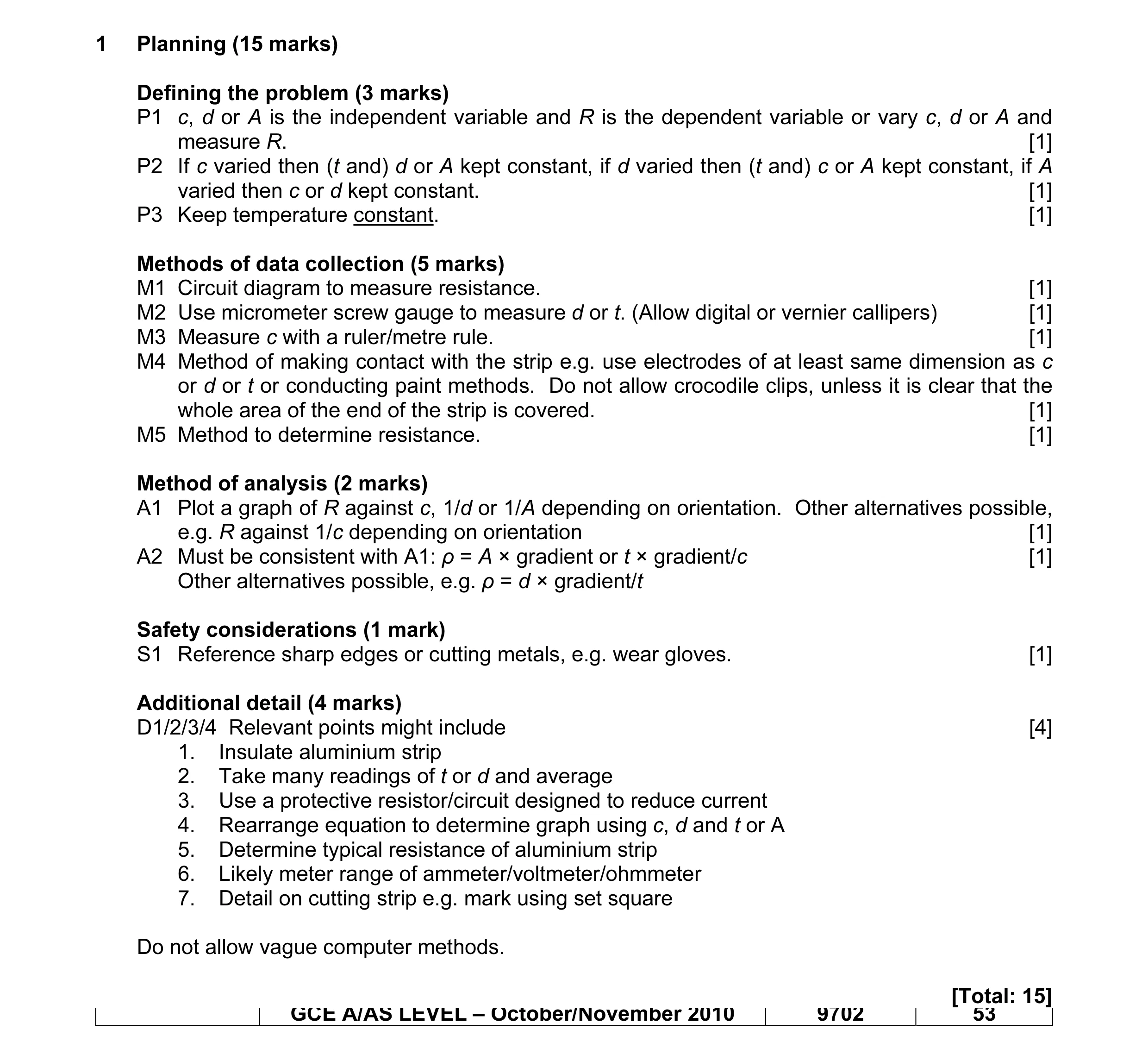 15
15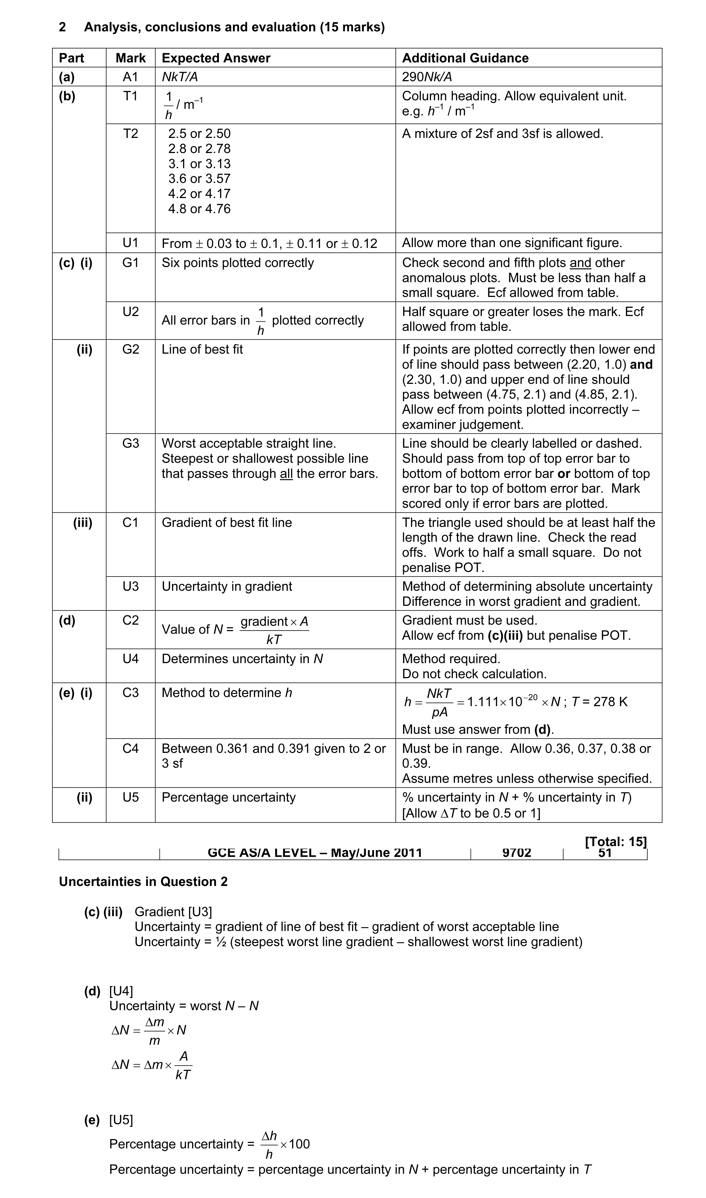 10
10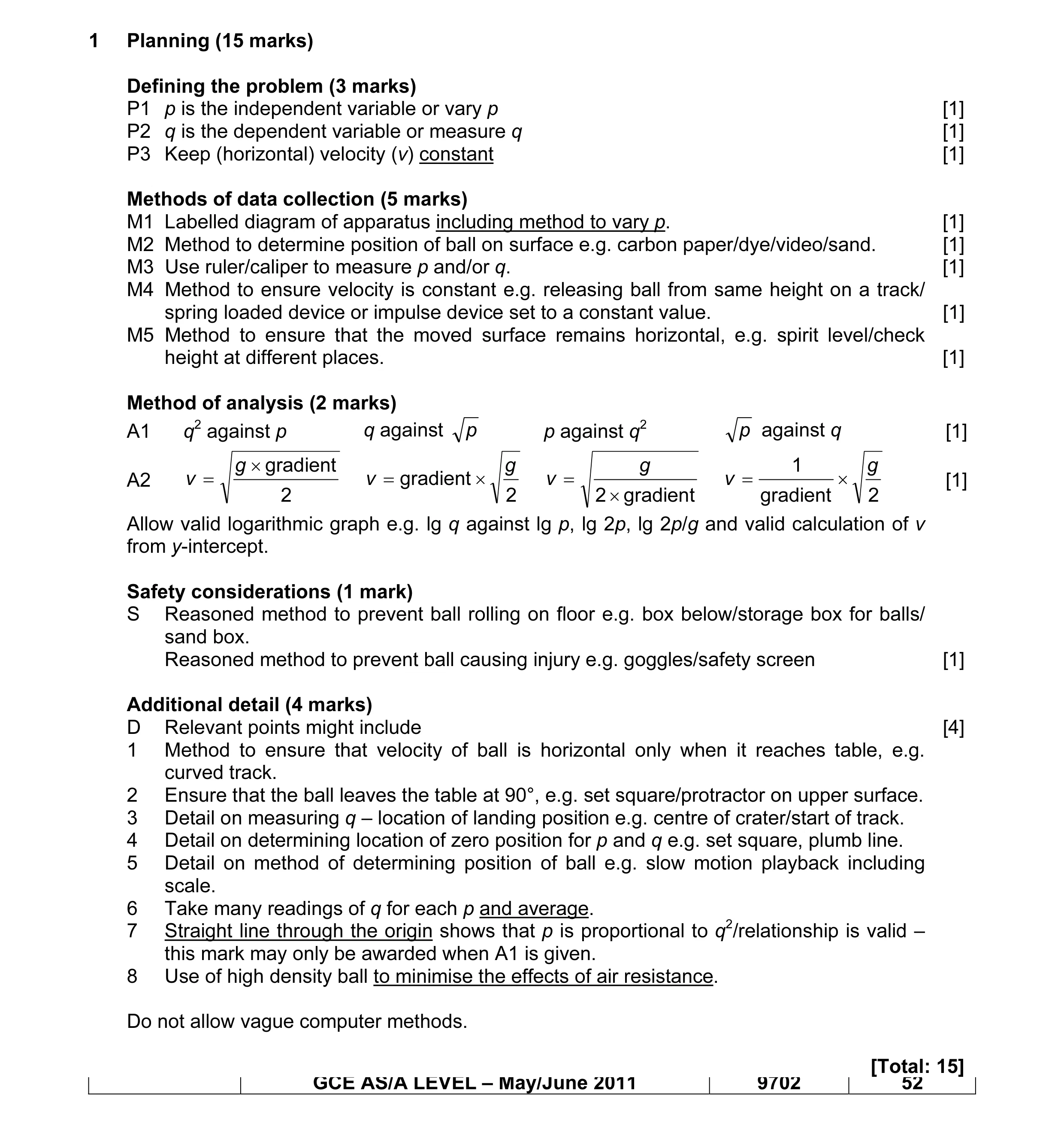 15
15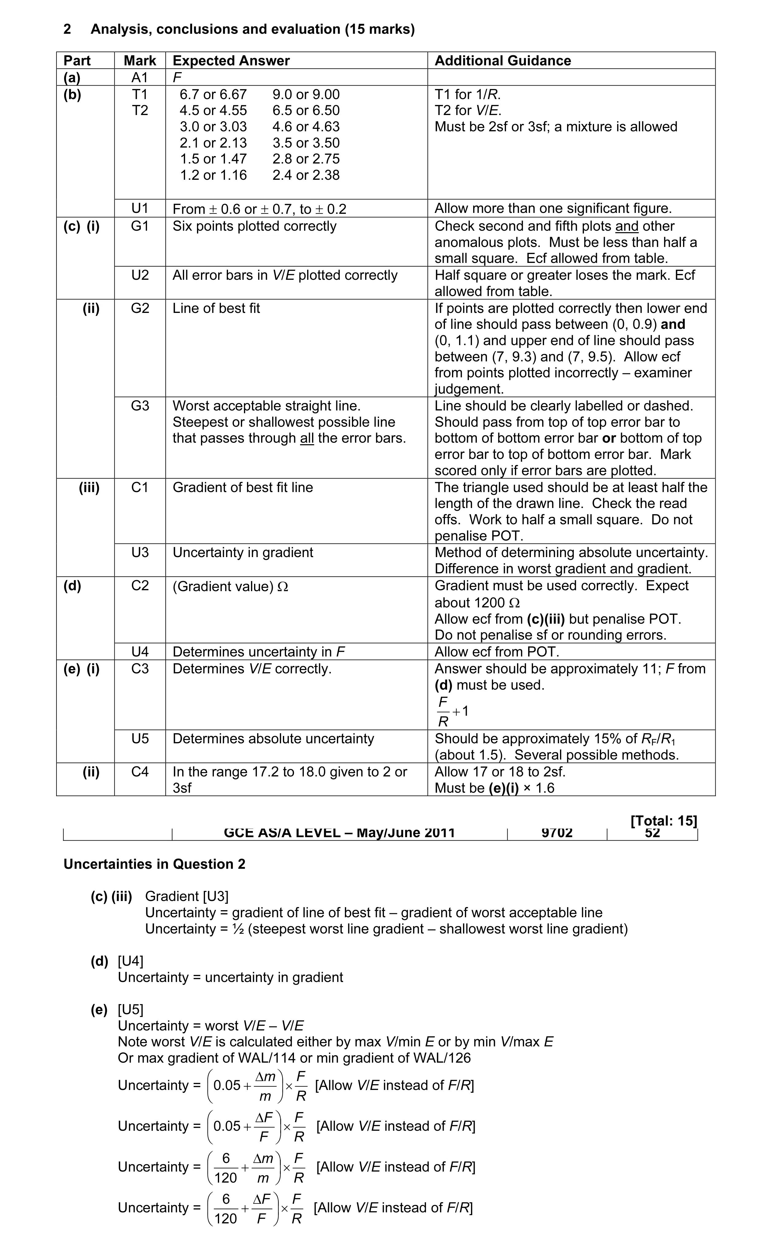 10
10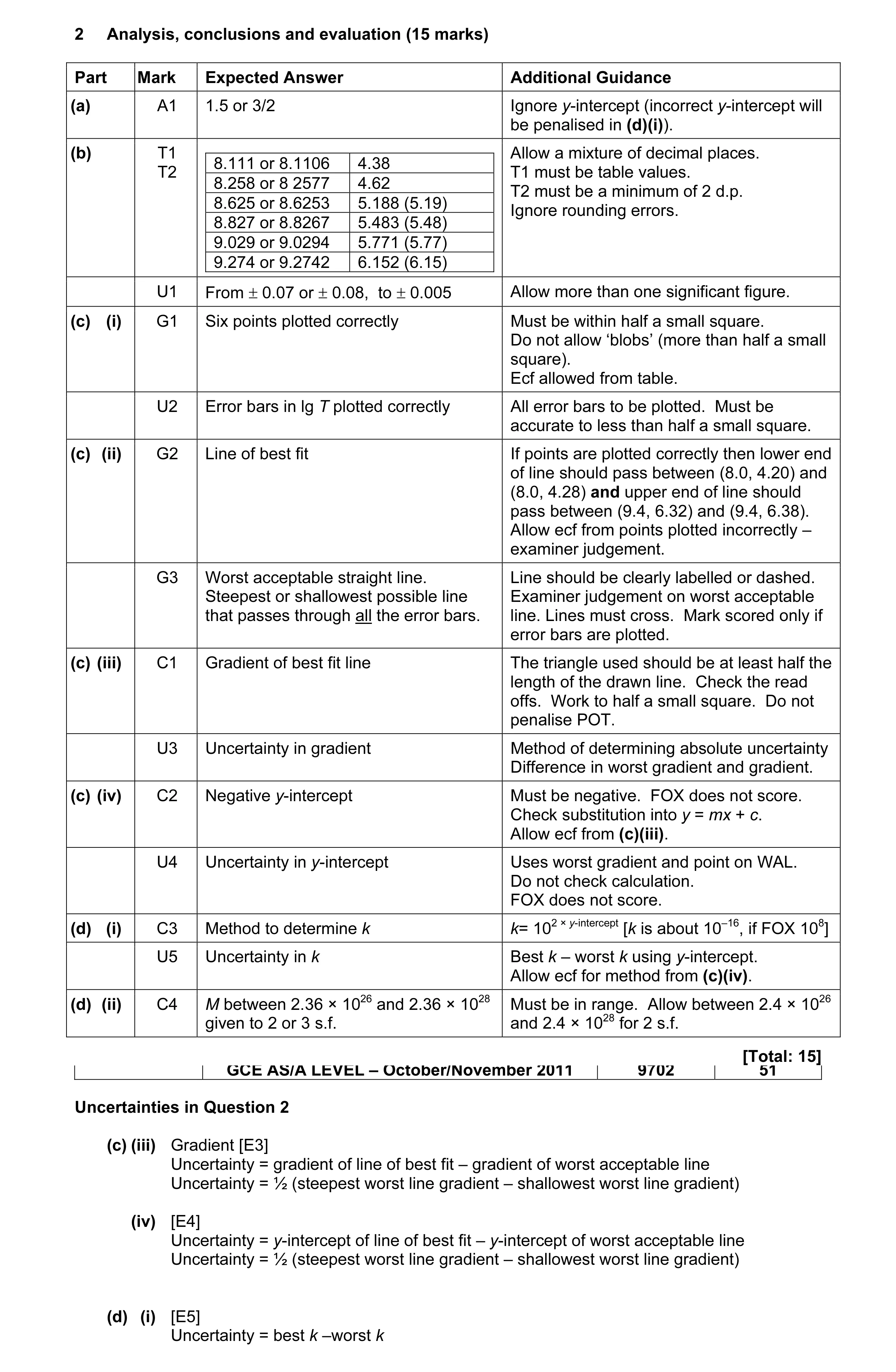 10
10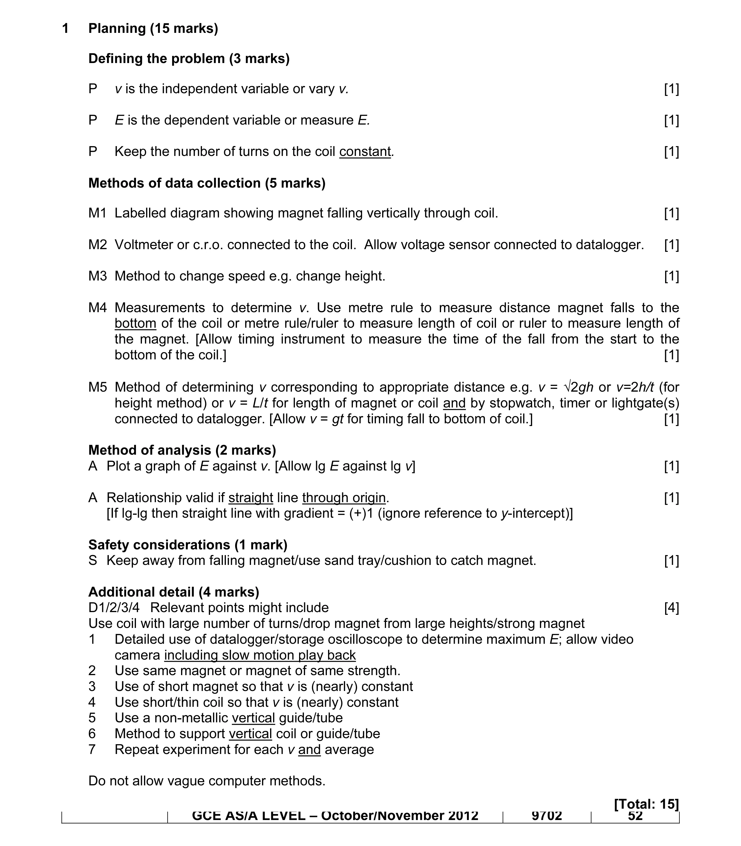 15
15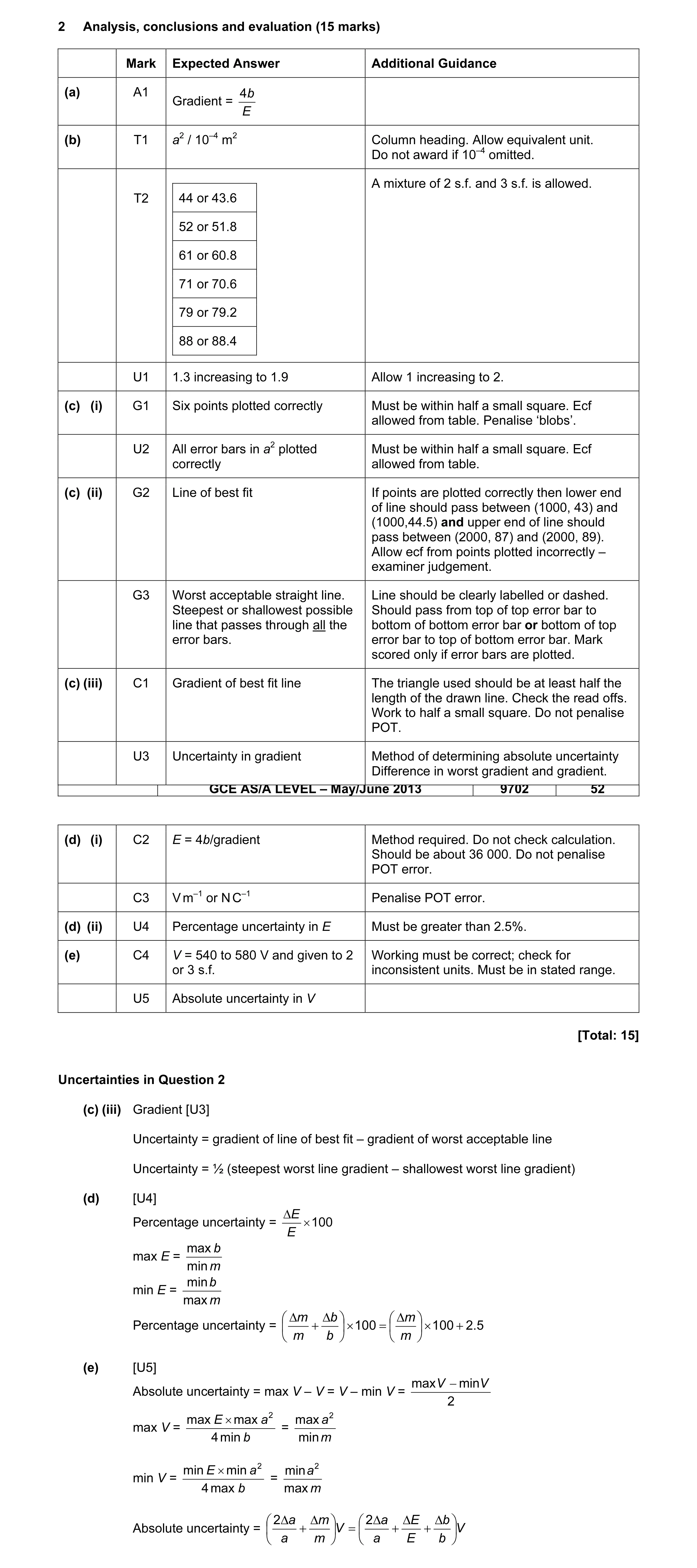 10
10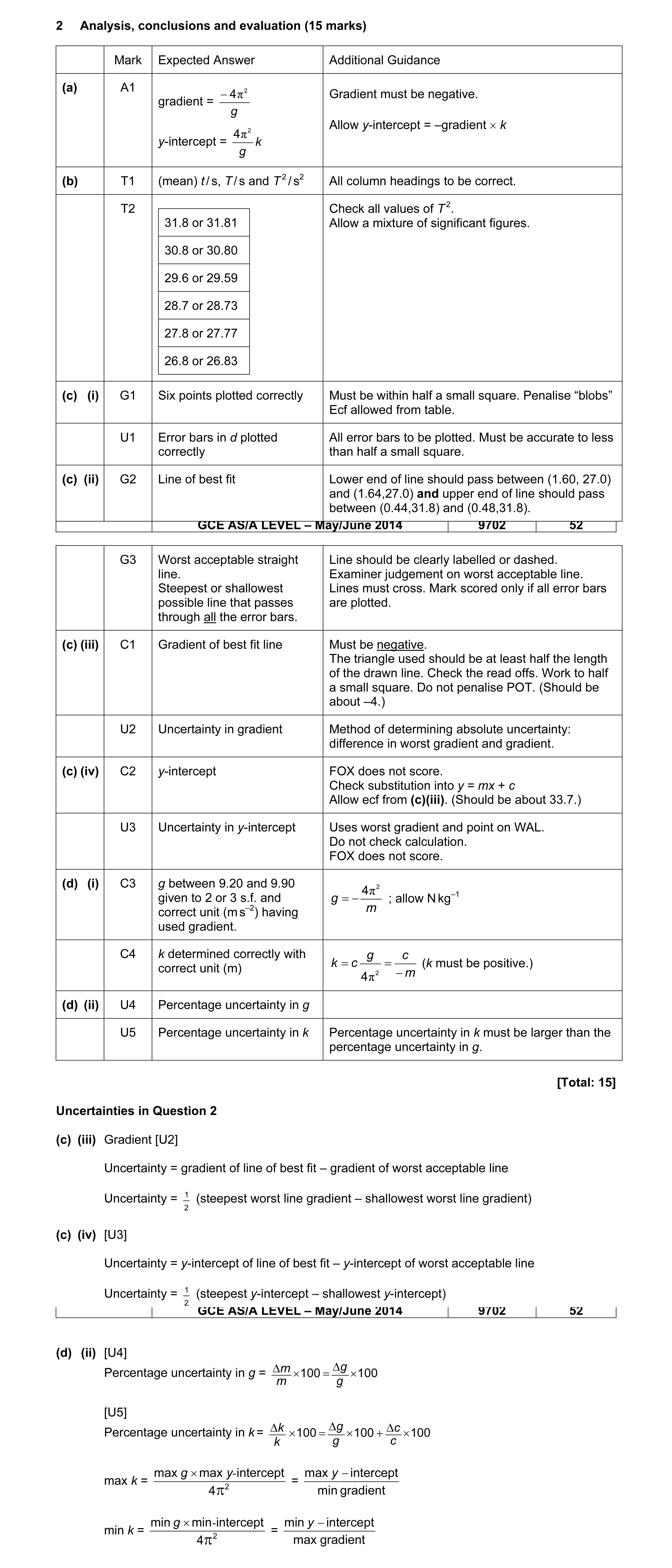 9
9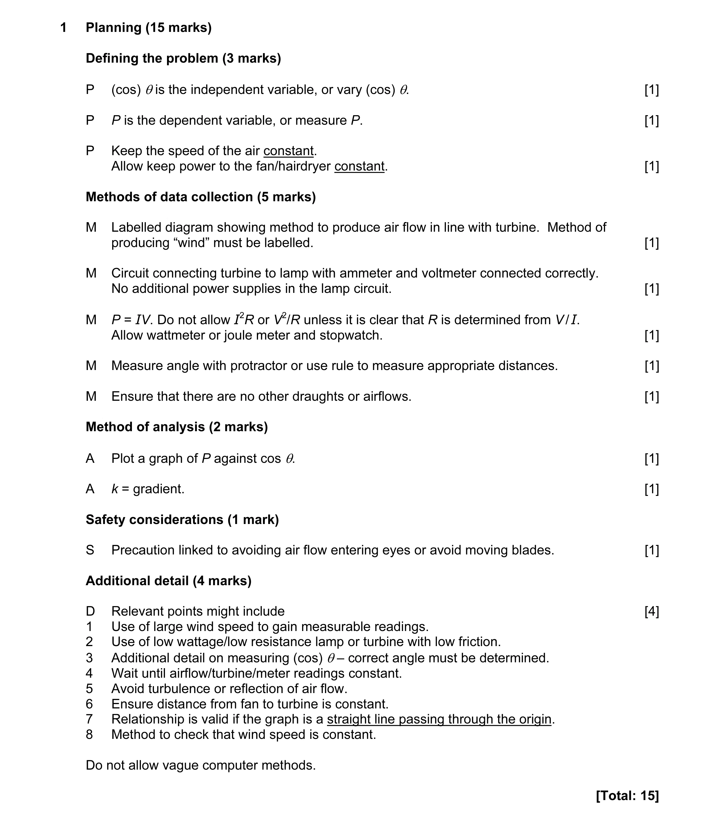 15
15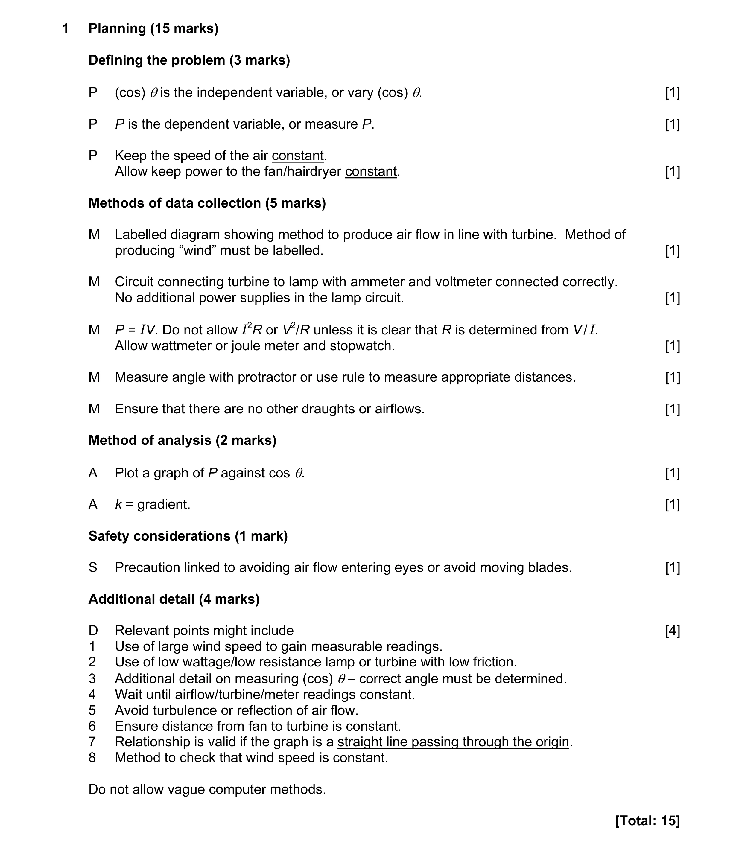 15
15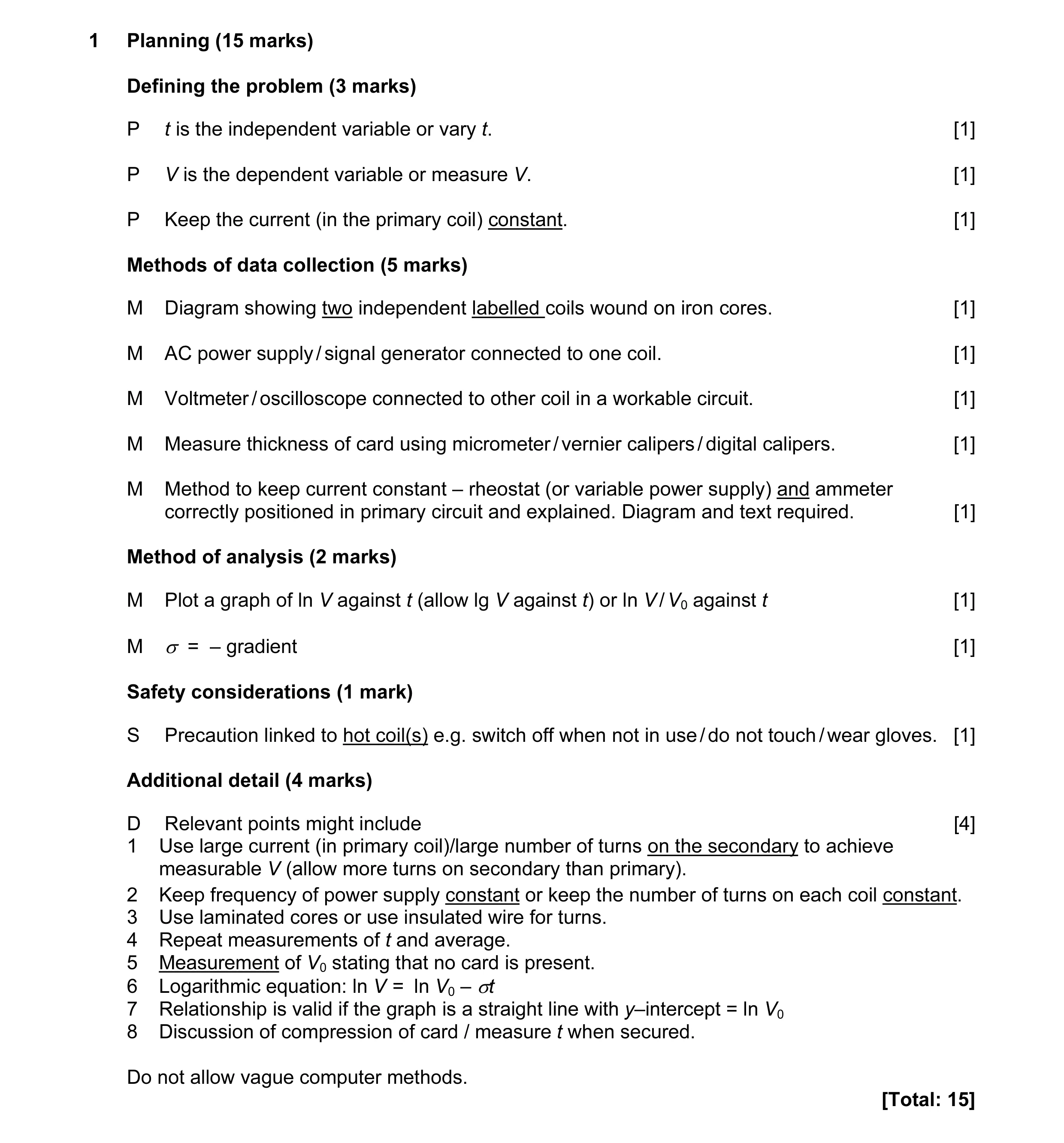 15
15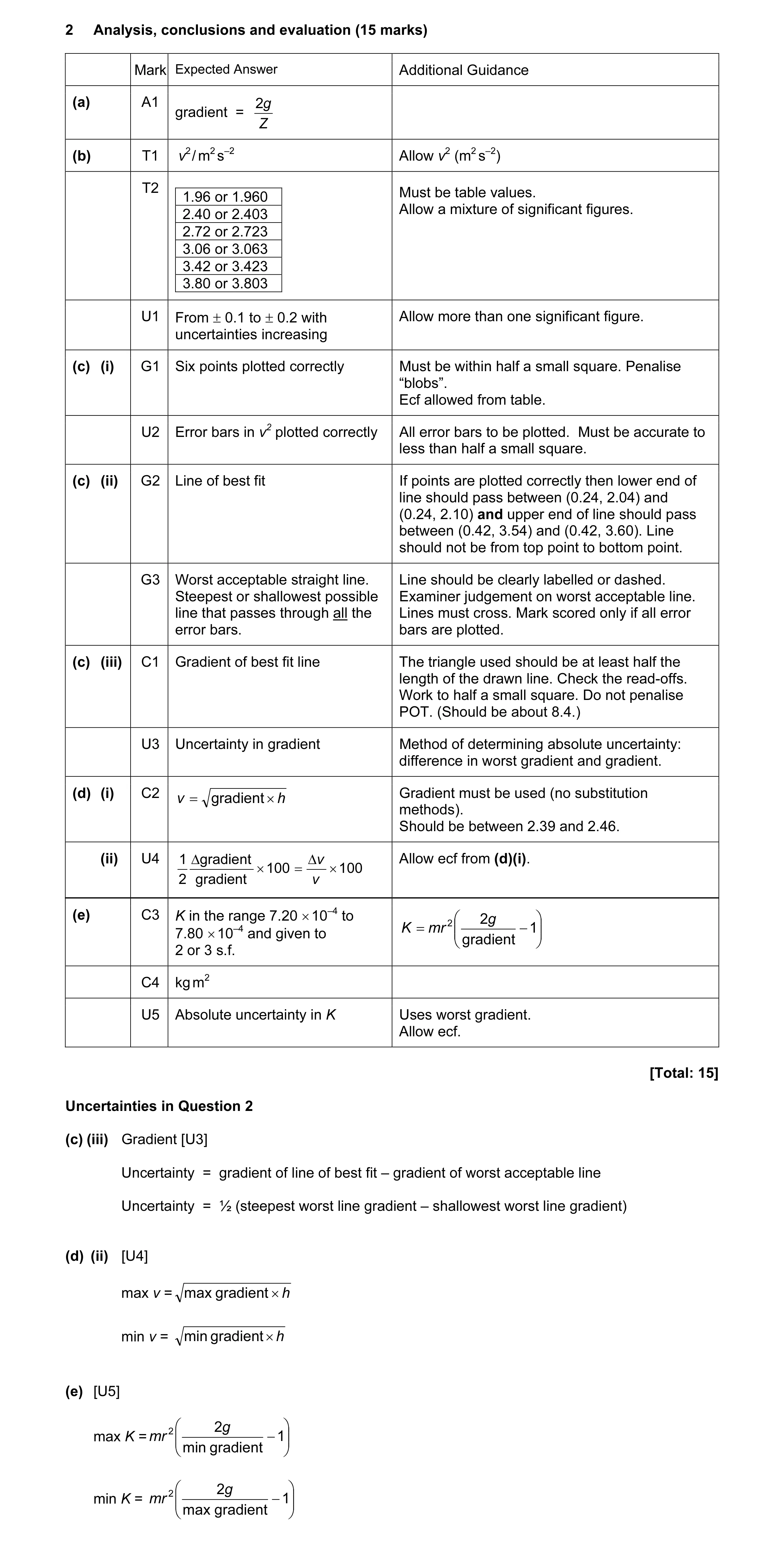 10
10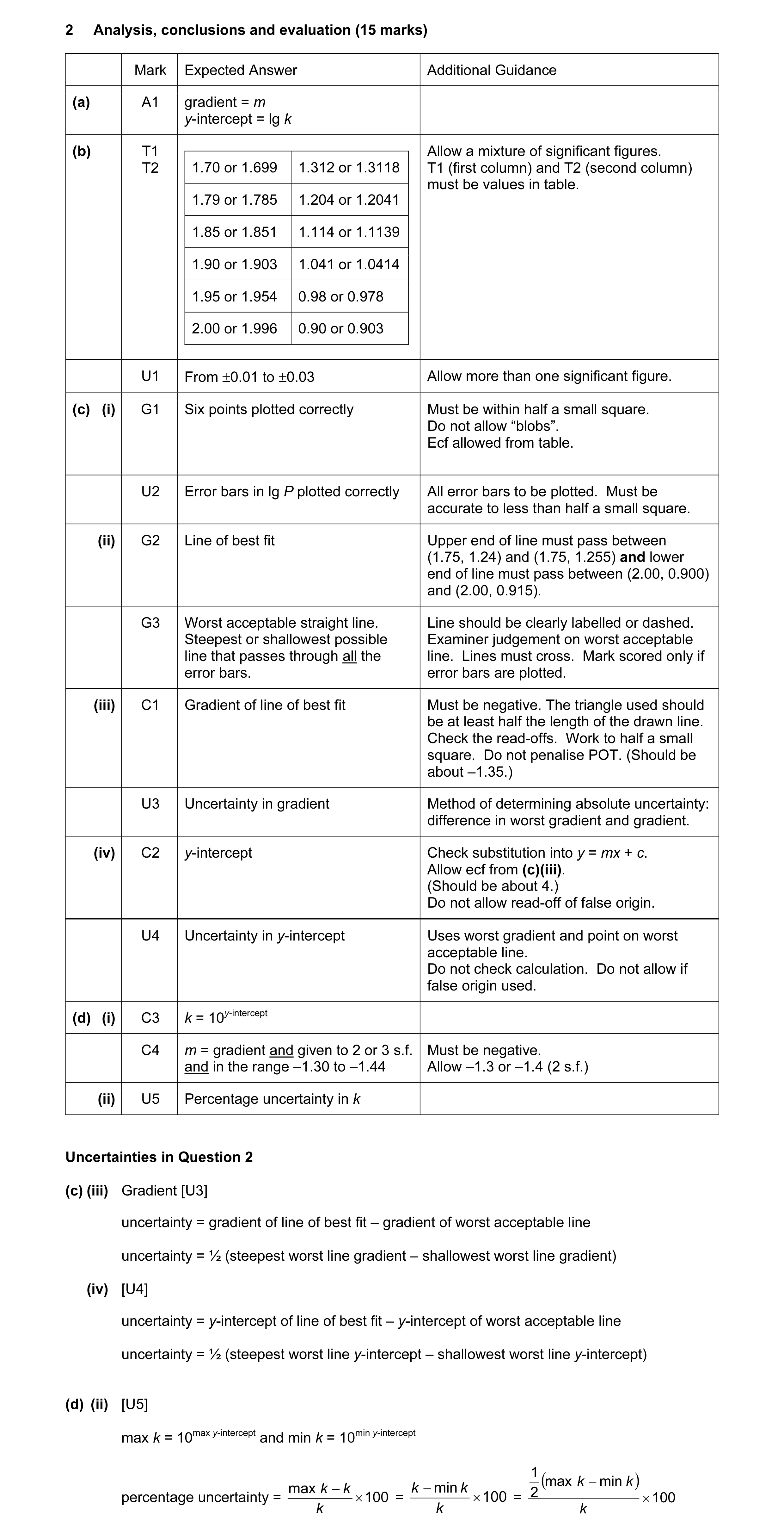 10
10 10
10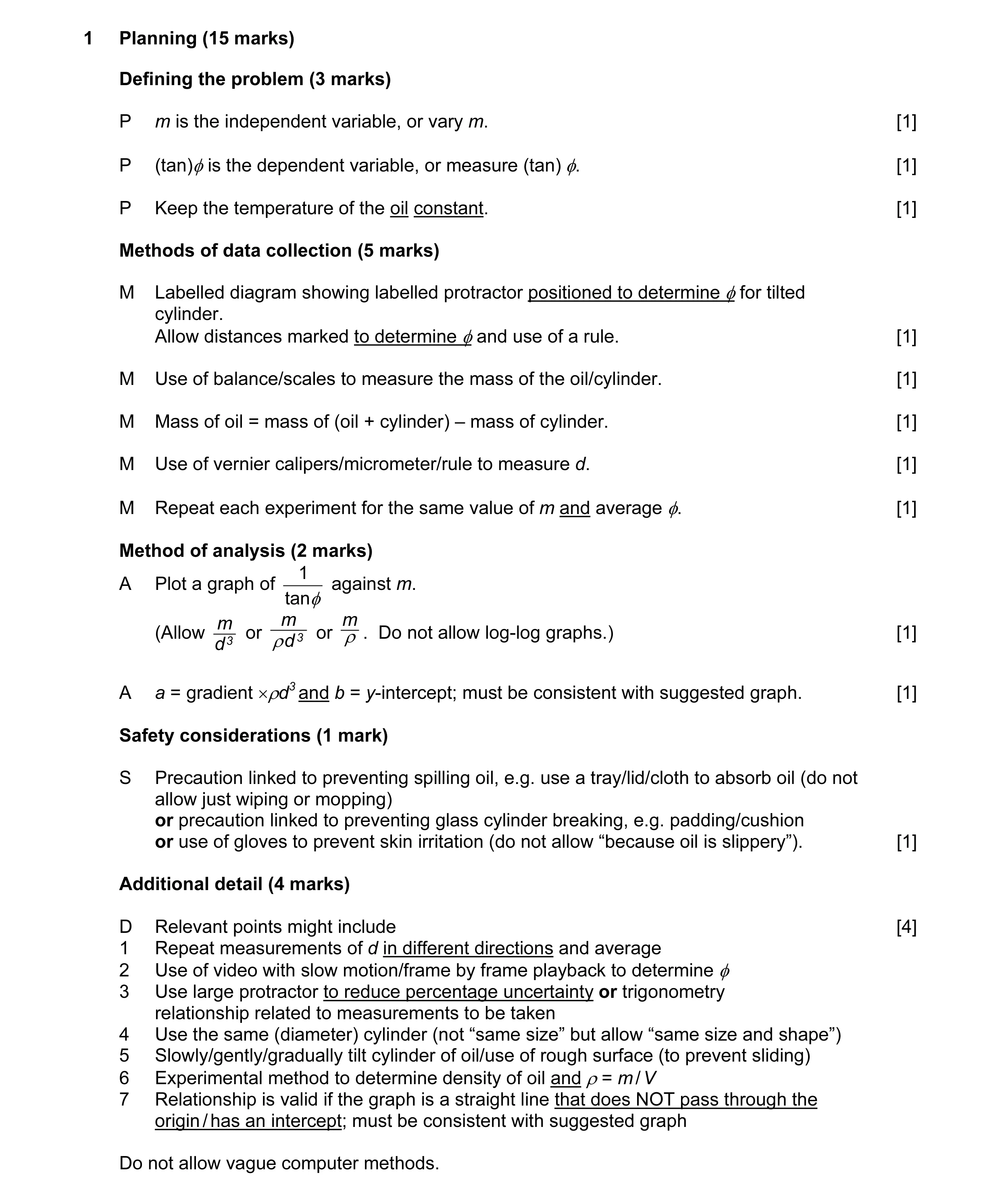 15
15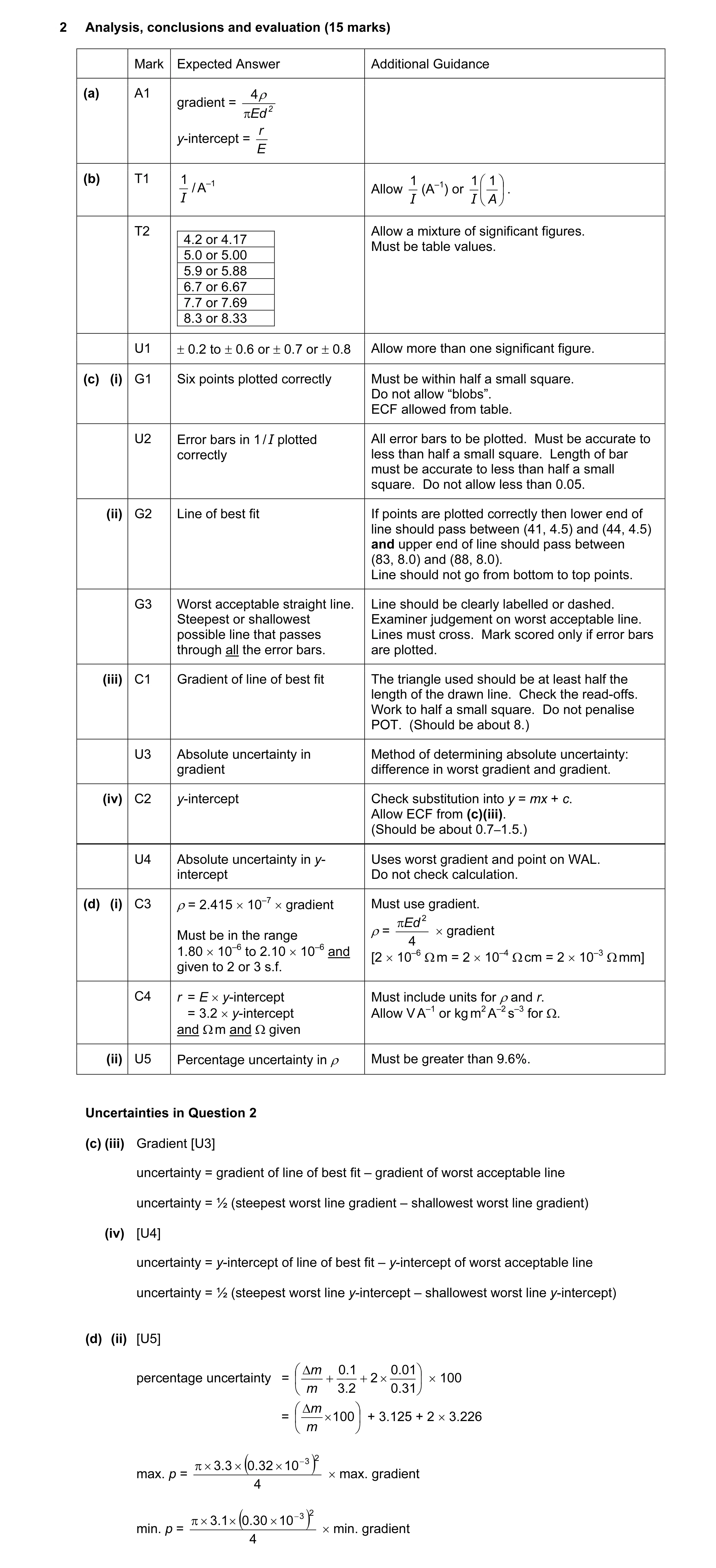 10
10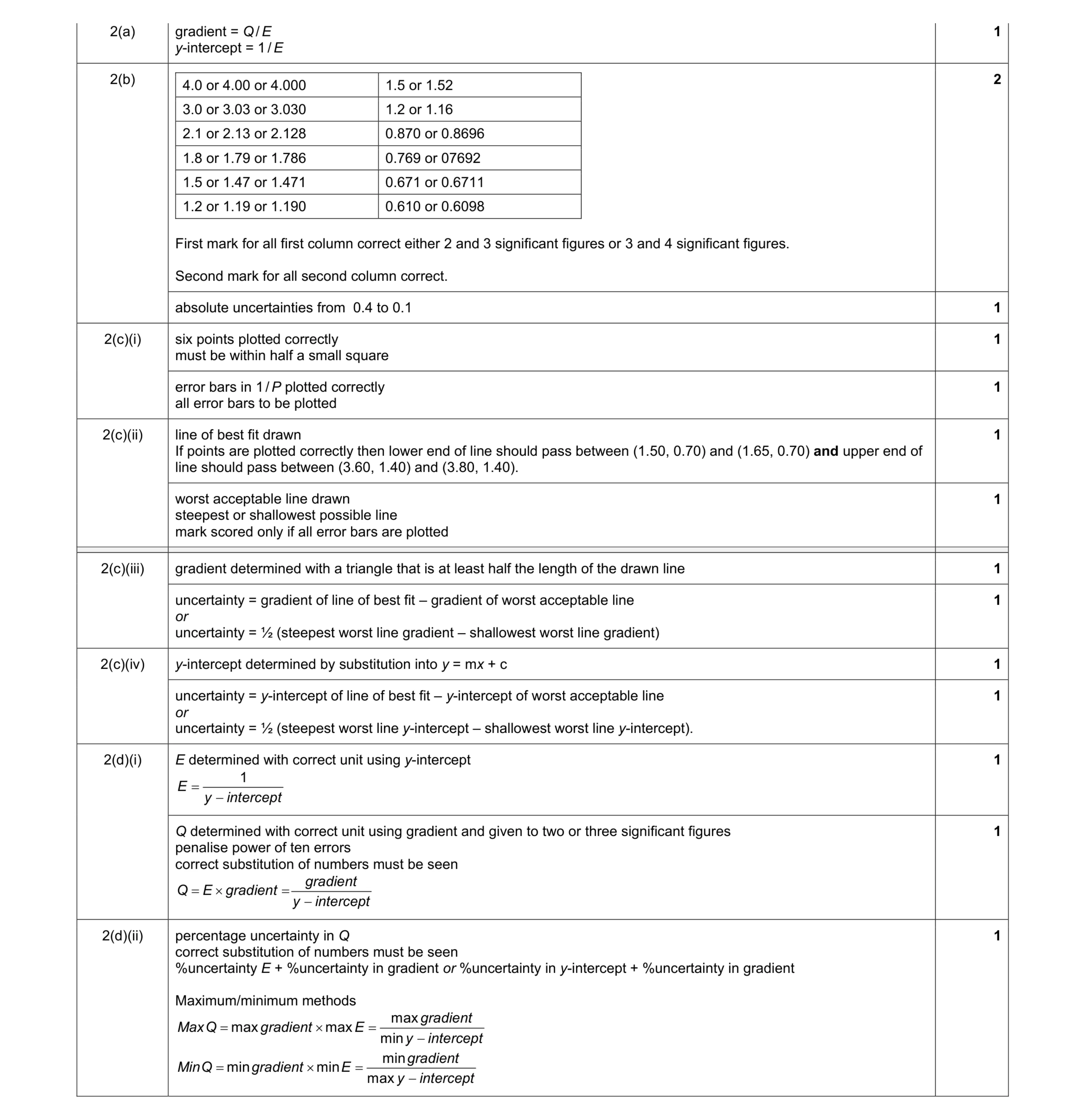 10
10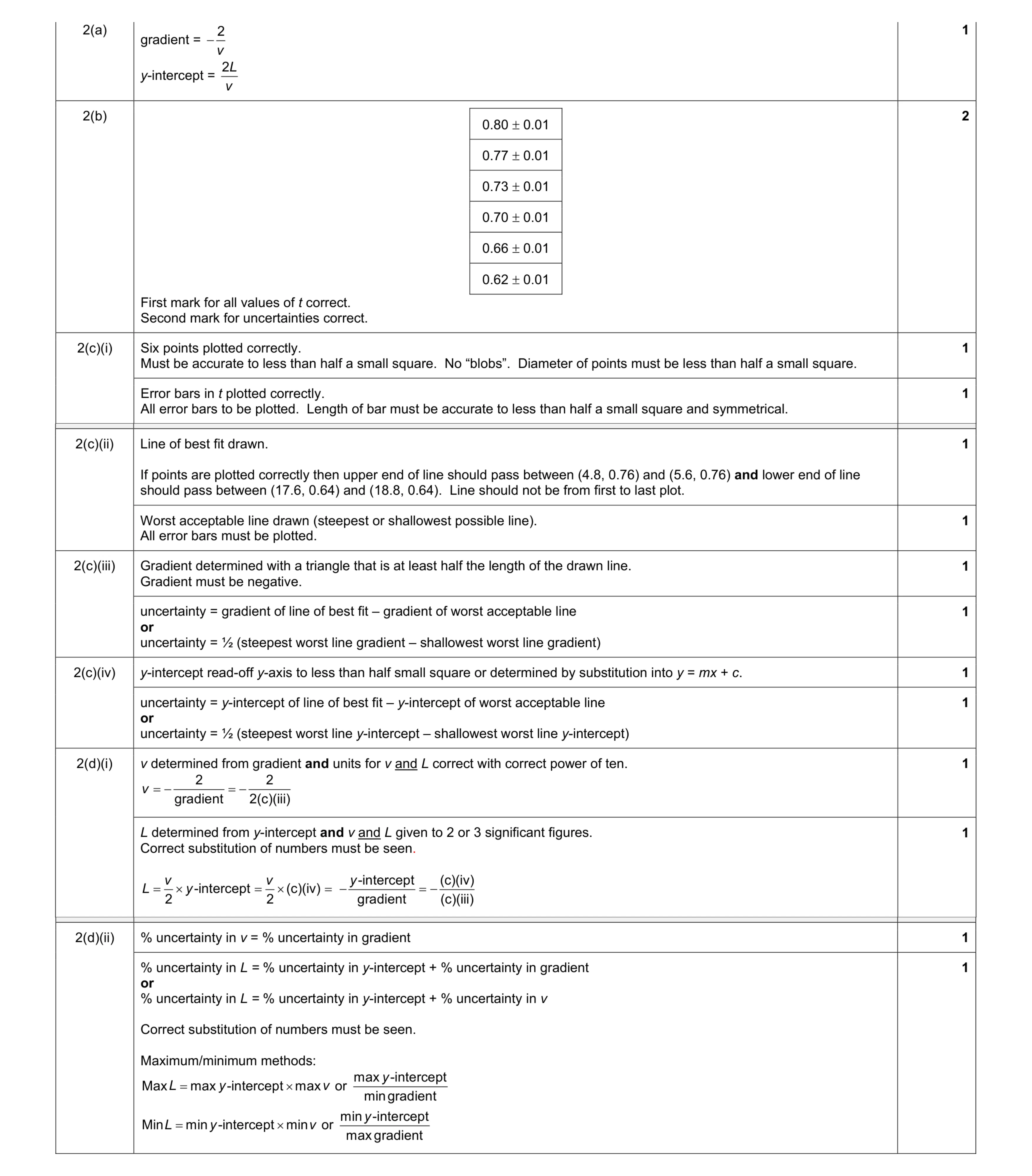 9
9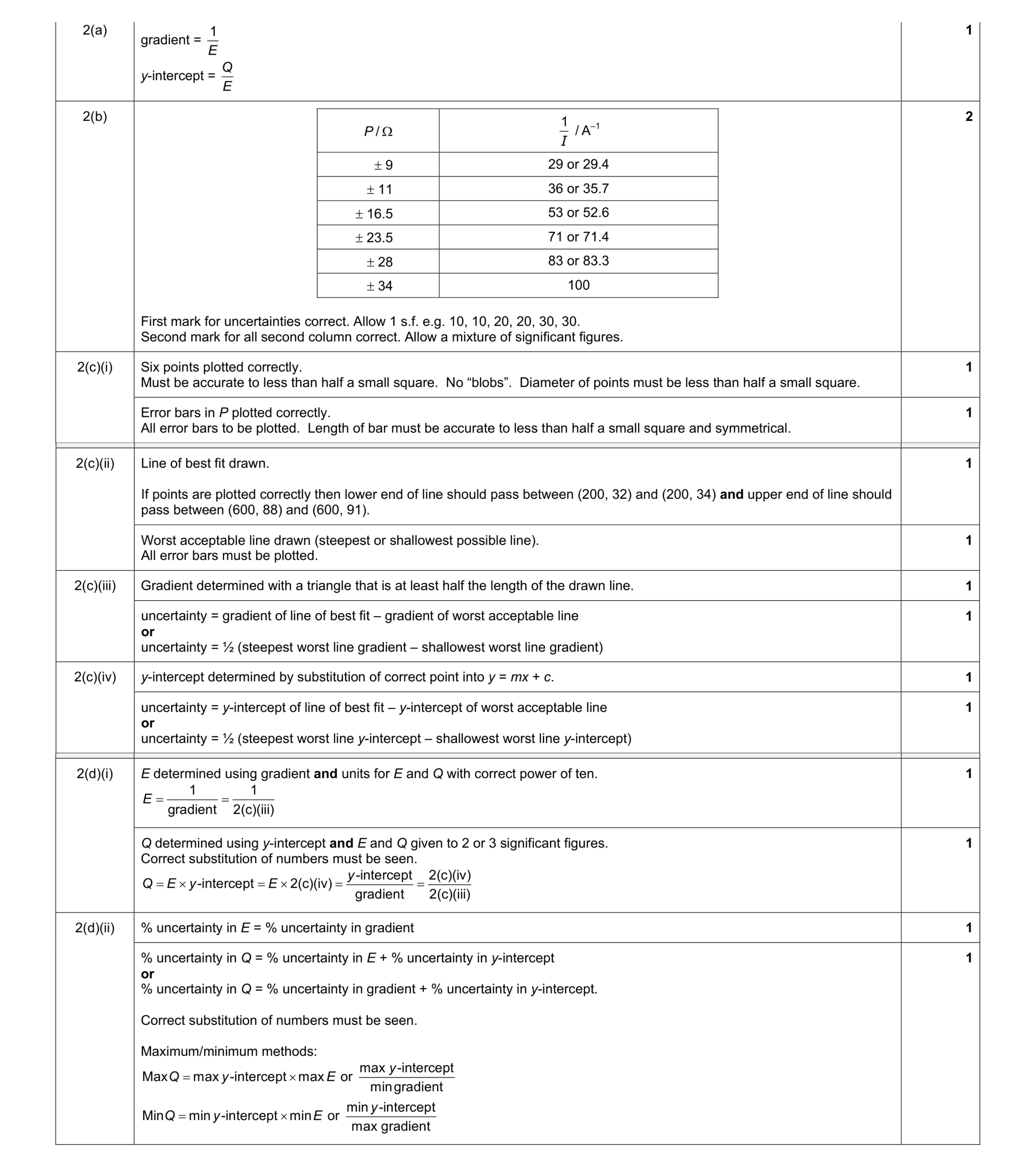 9
9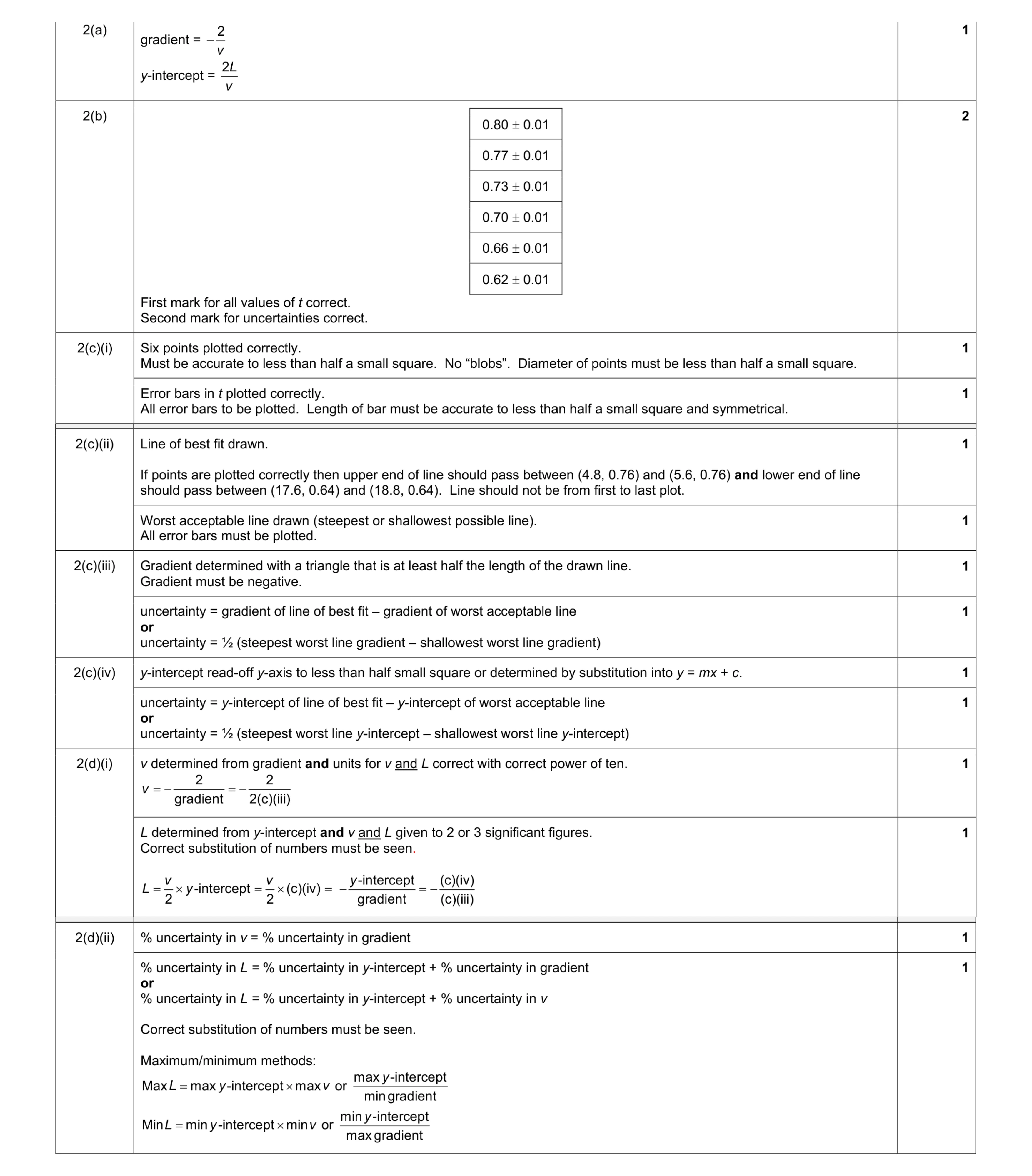 9
9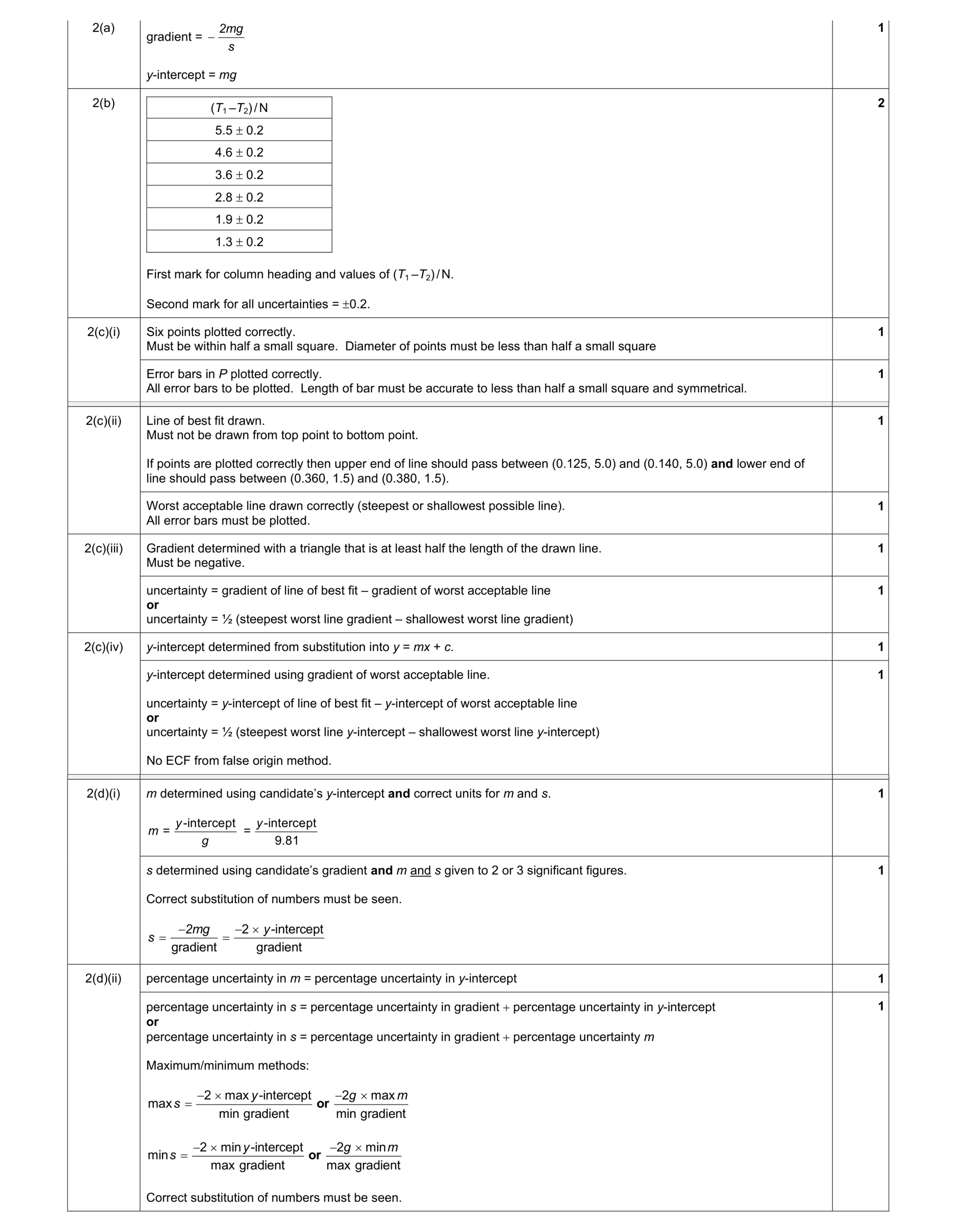 9
9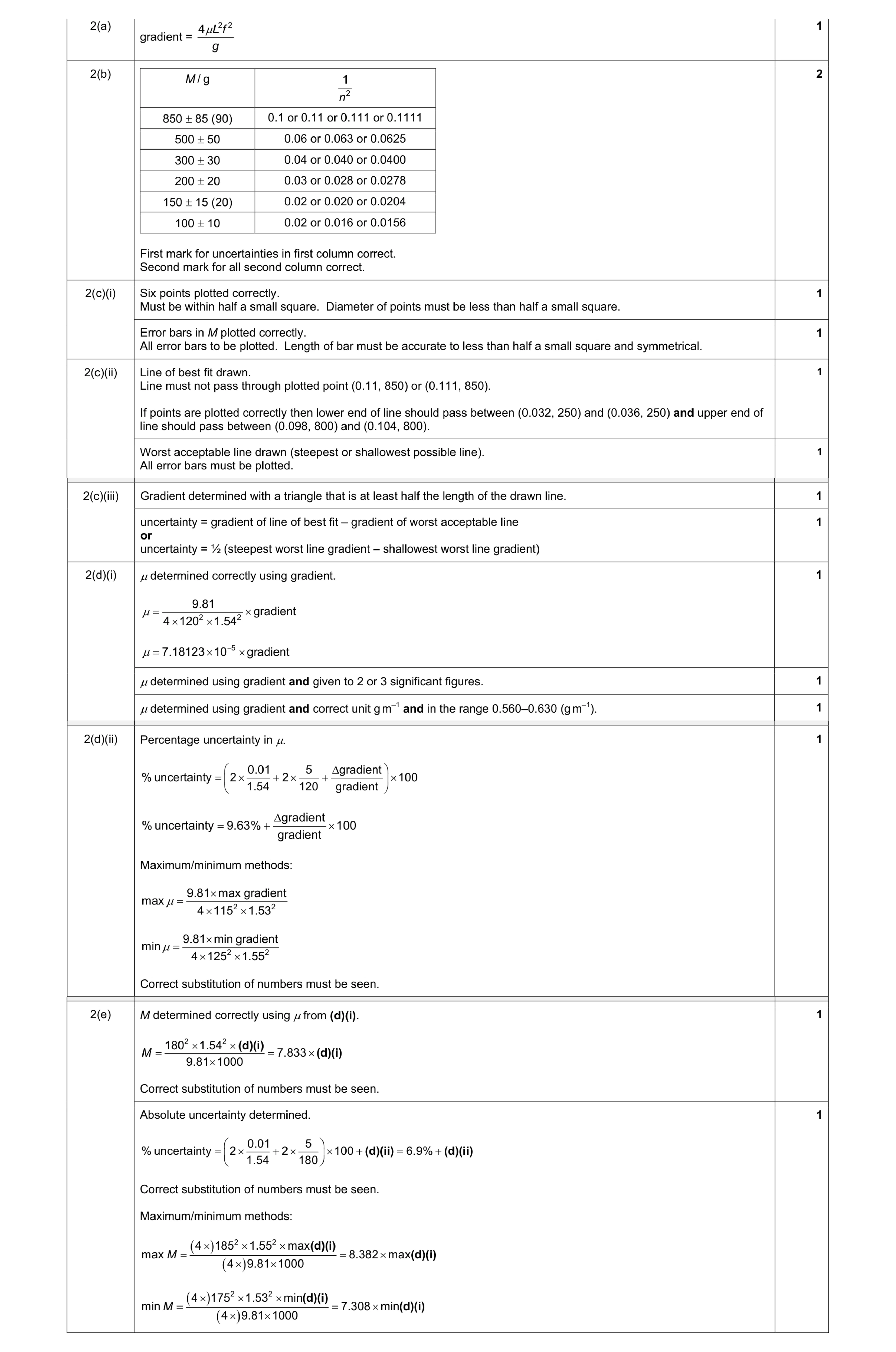 9
9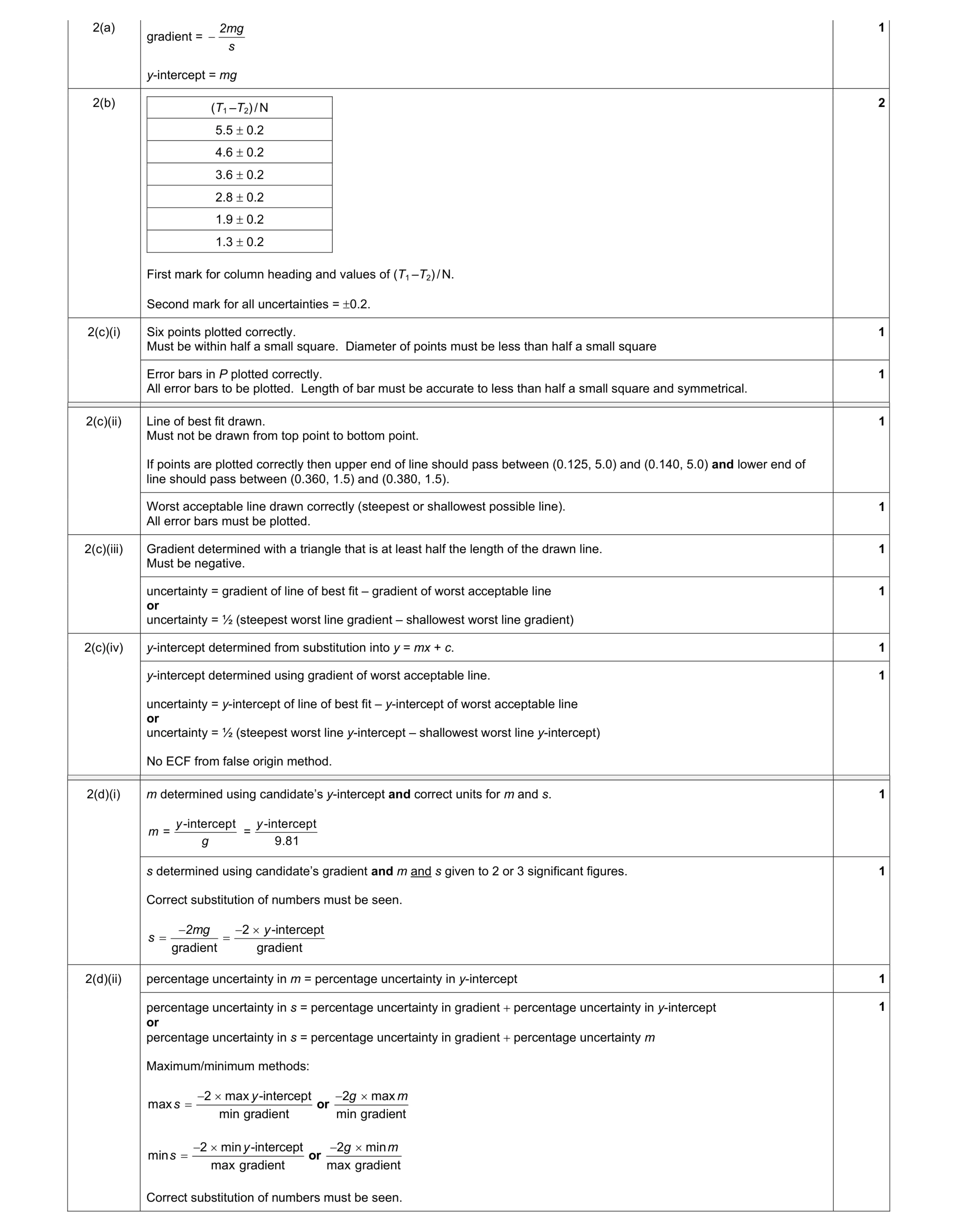 9
9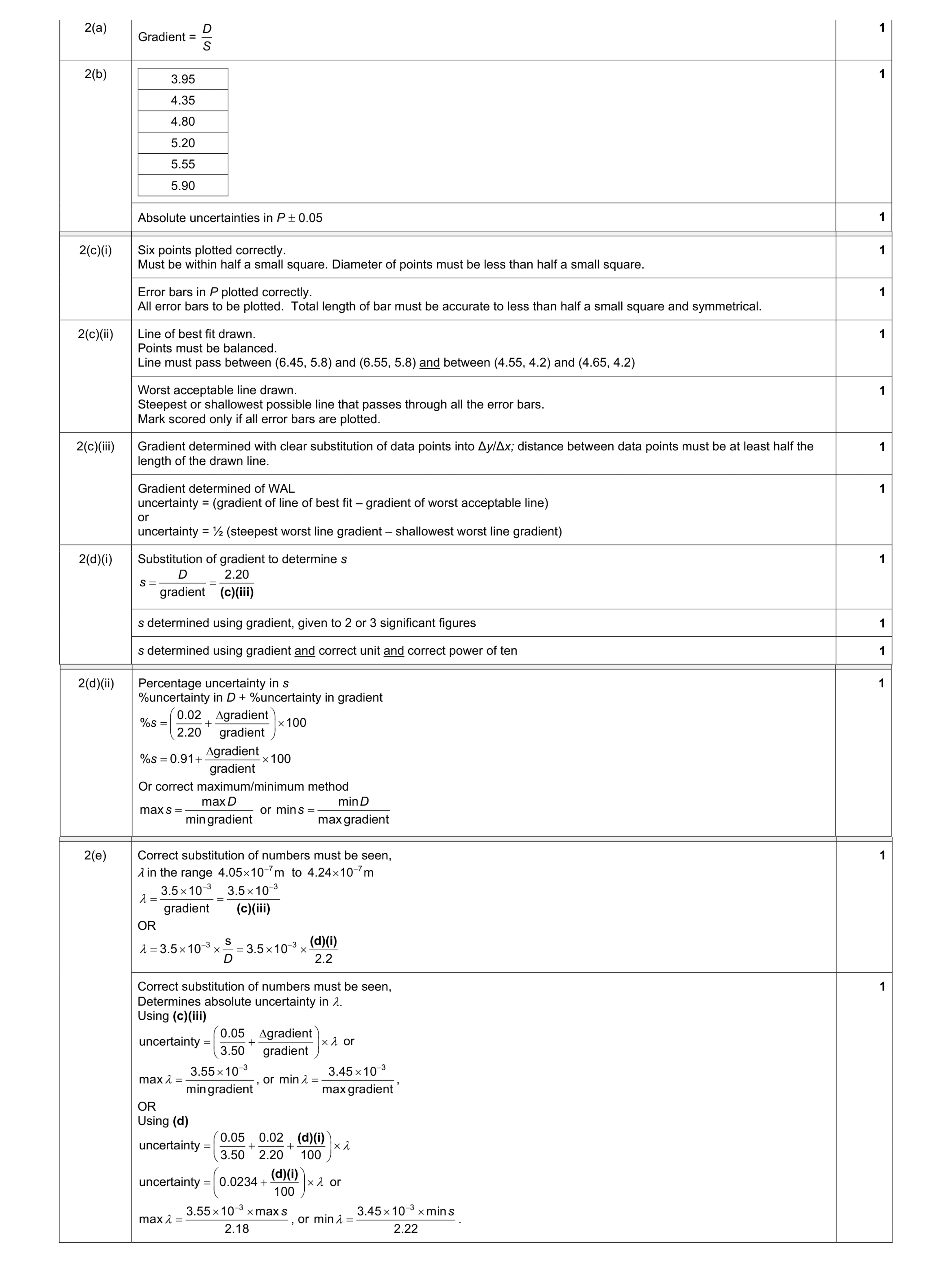 9
9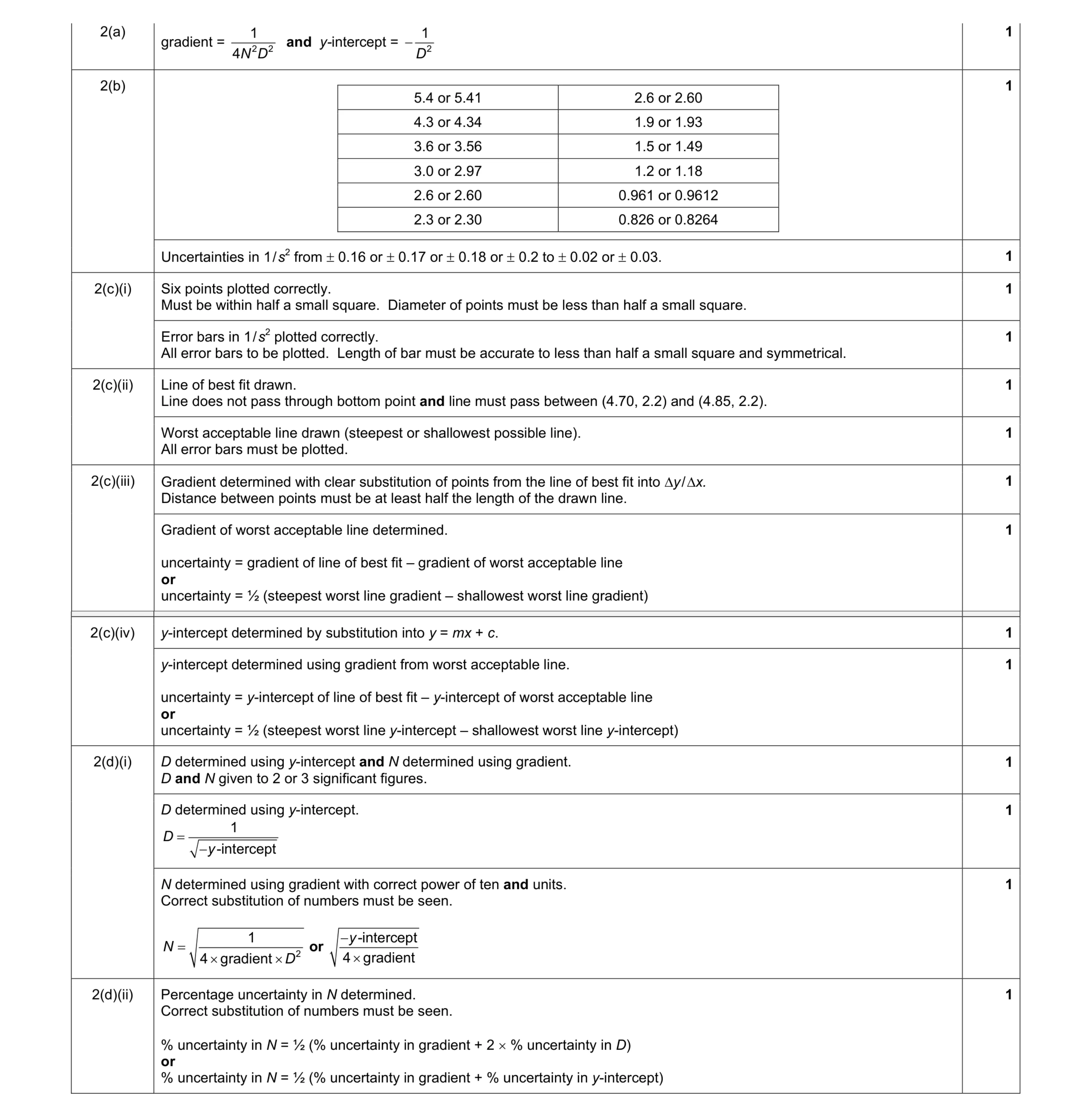 9
9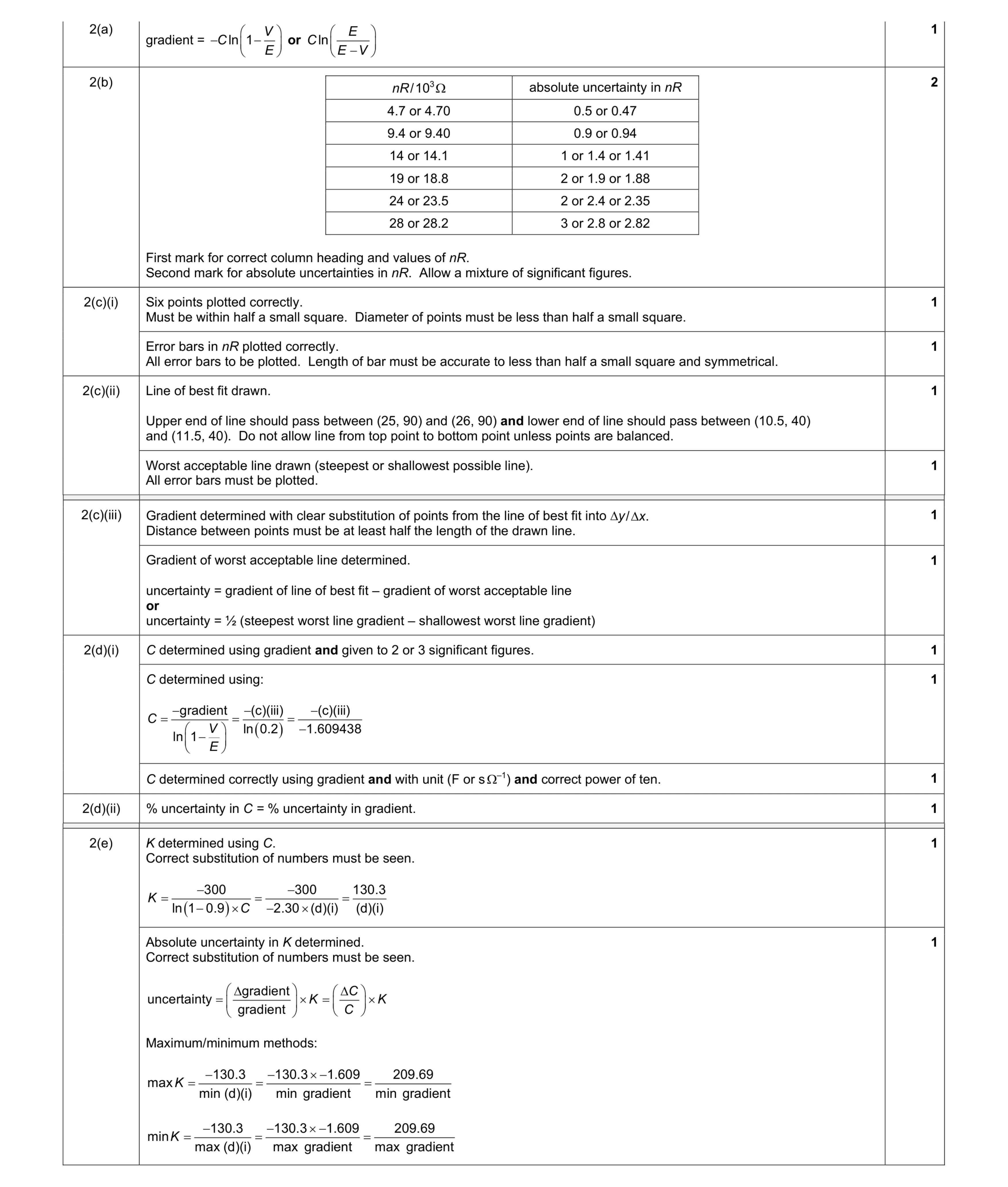 9
9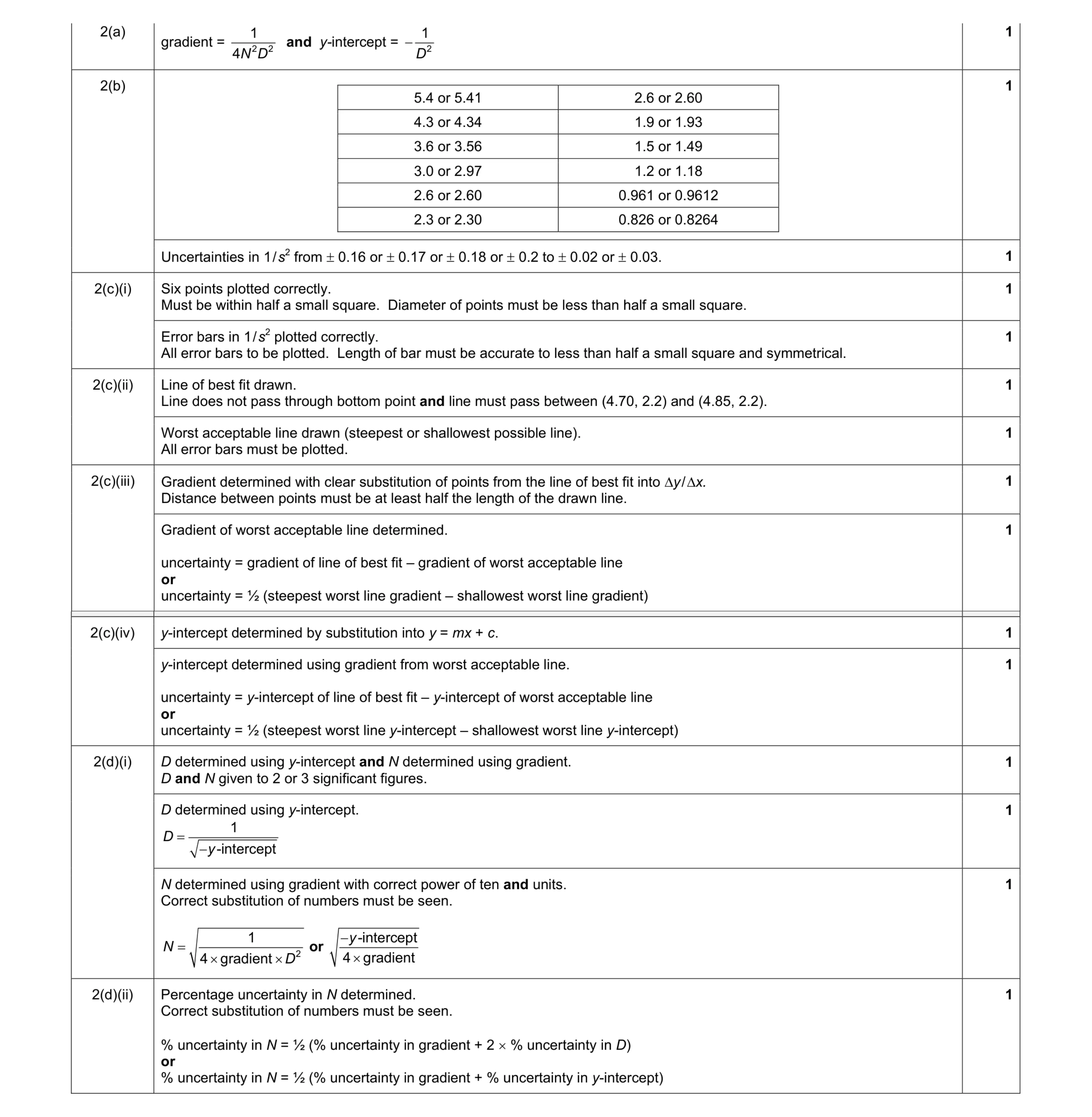 9
9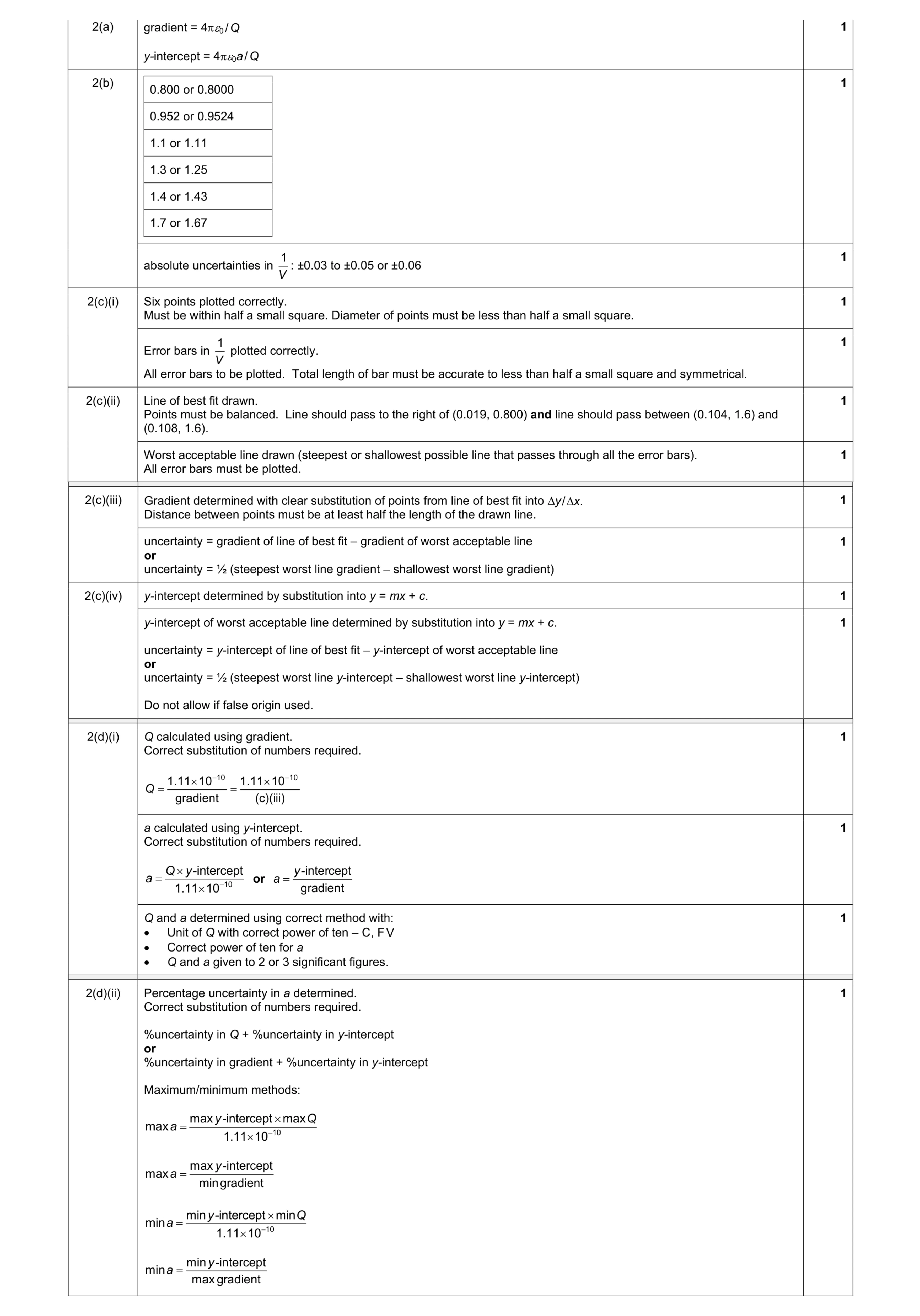 9
9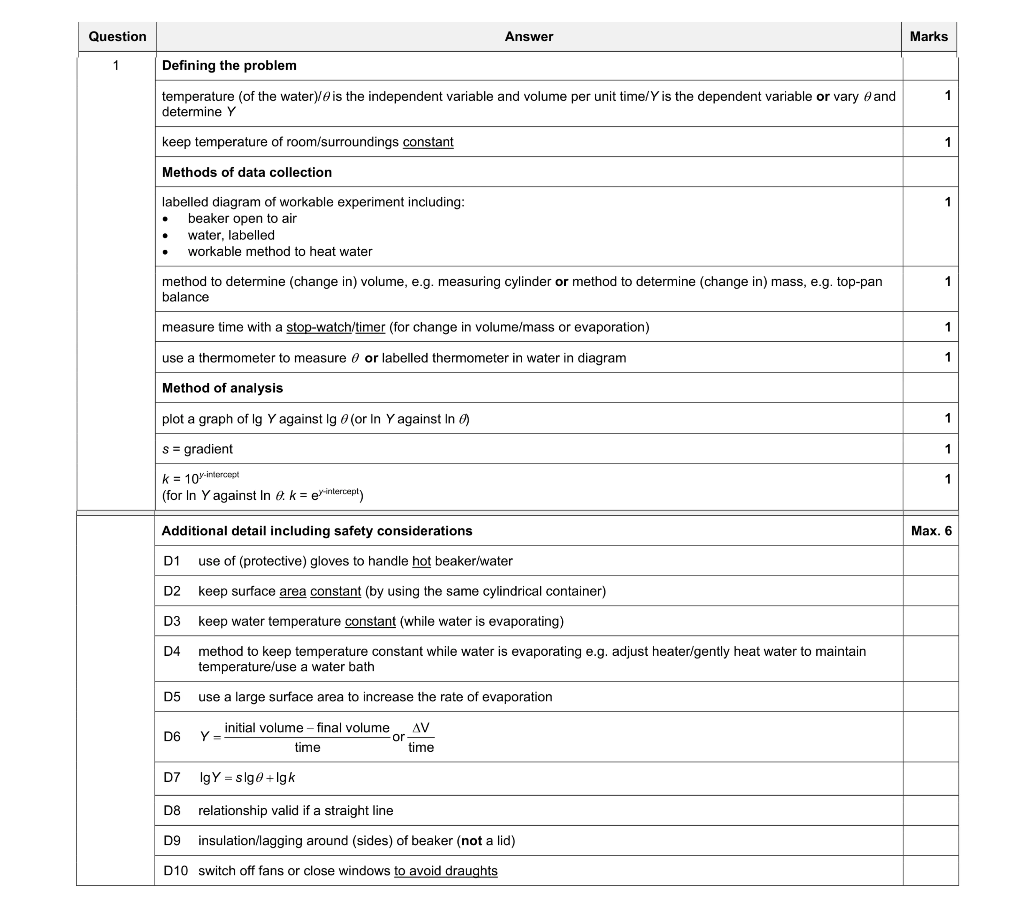 15
15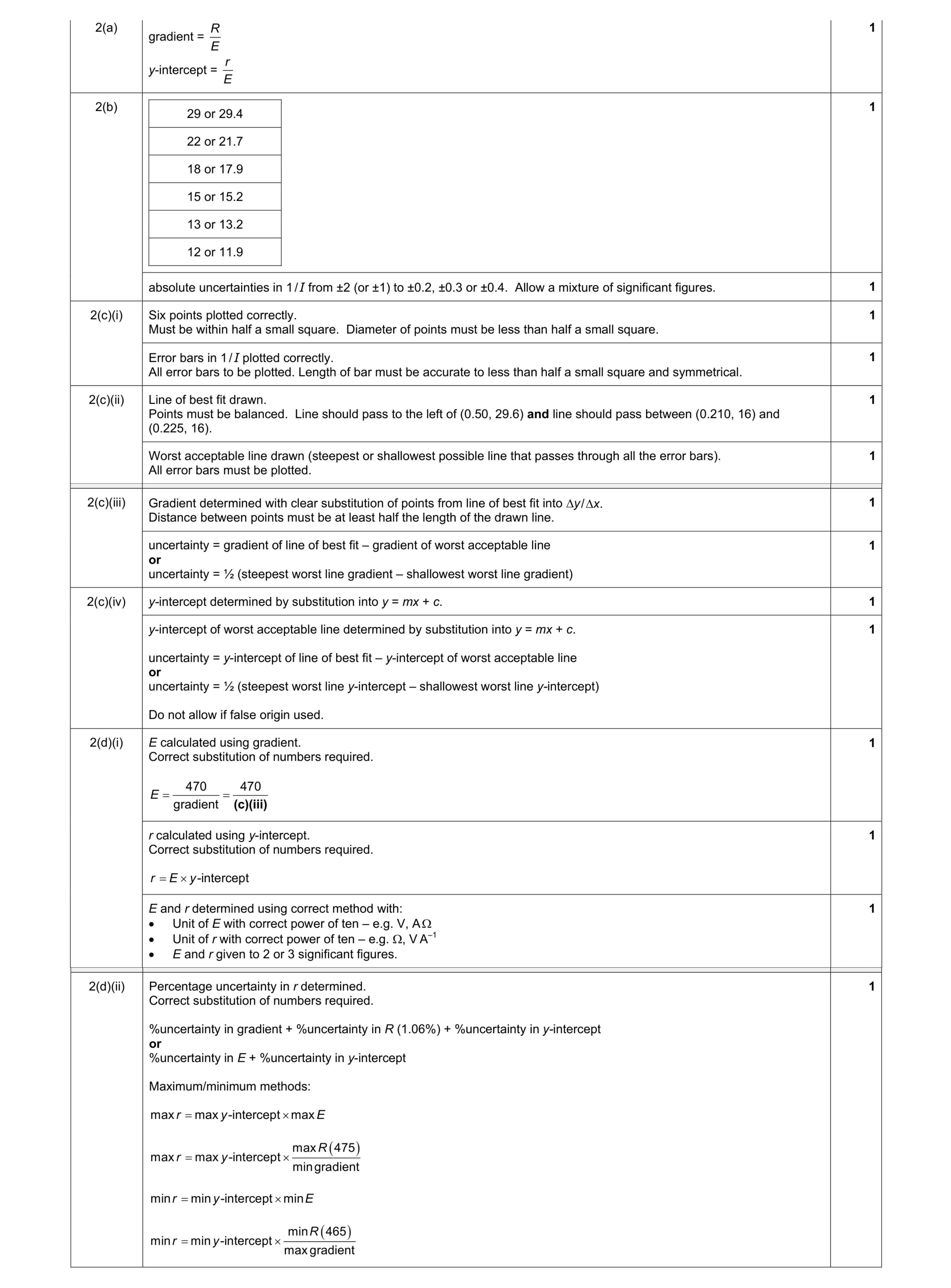 9
9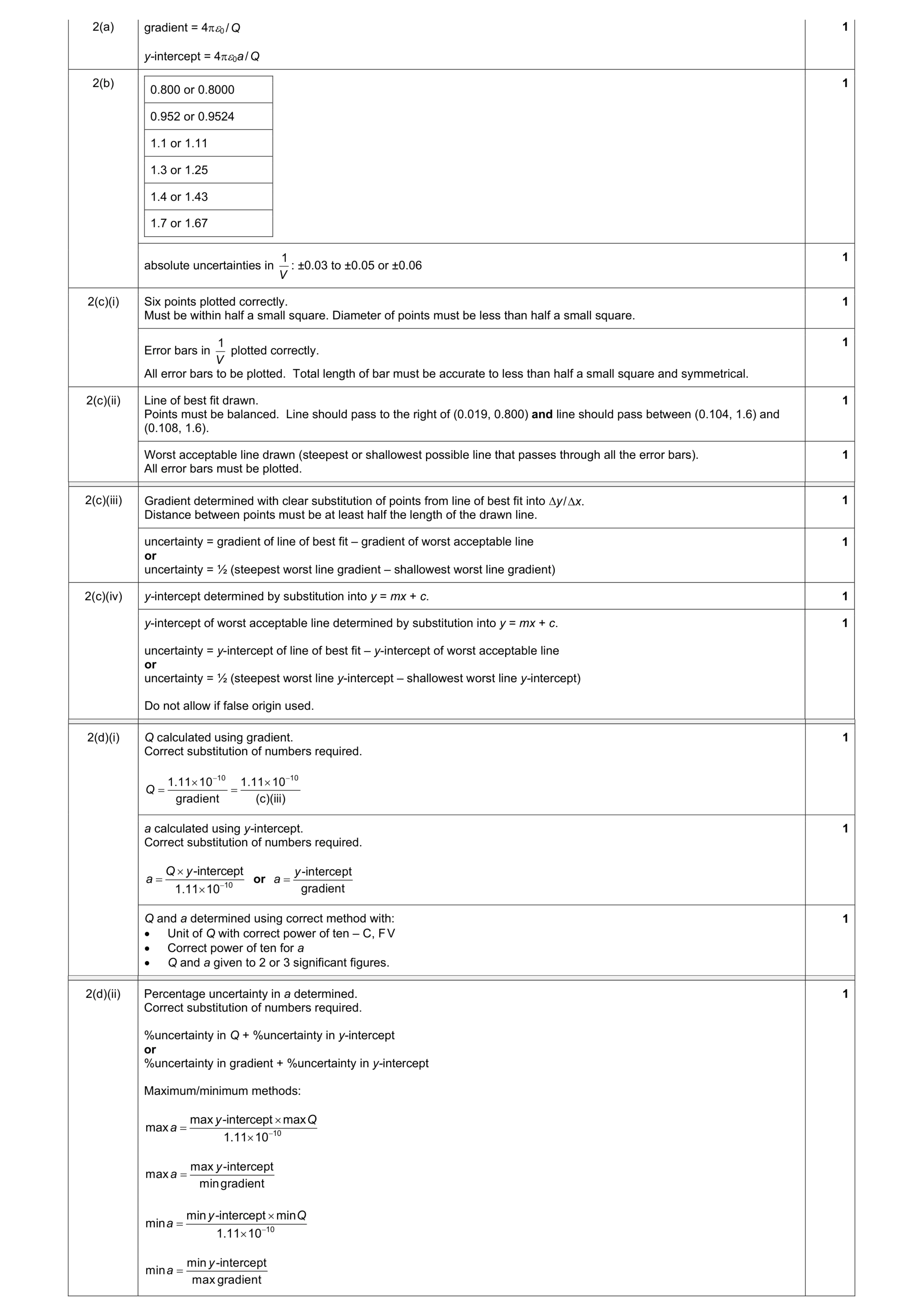 9
9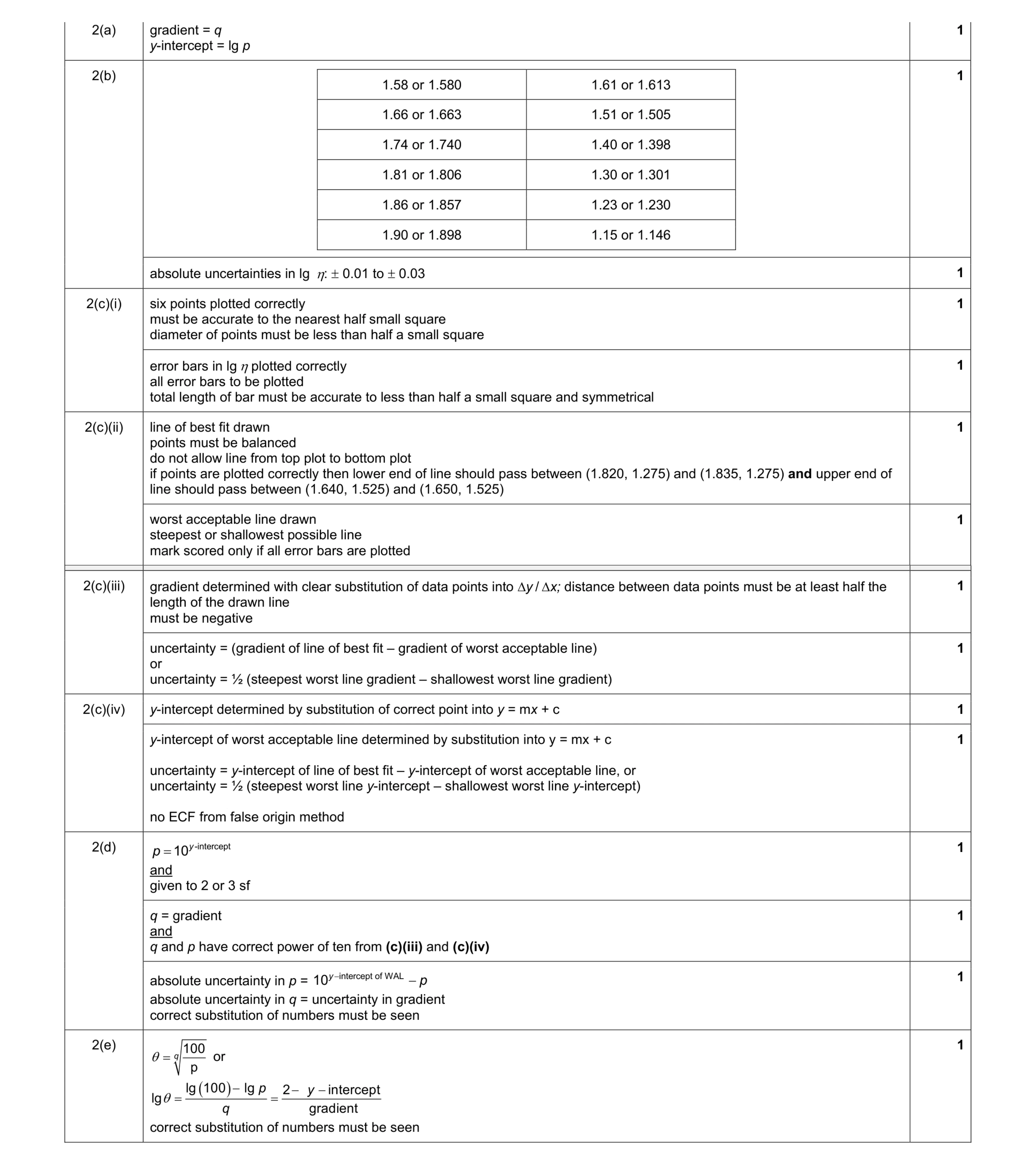 9
9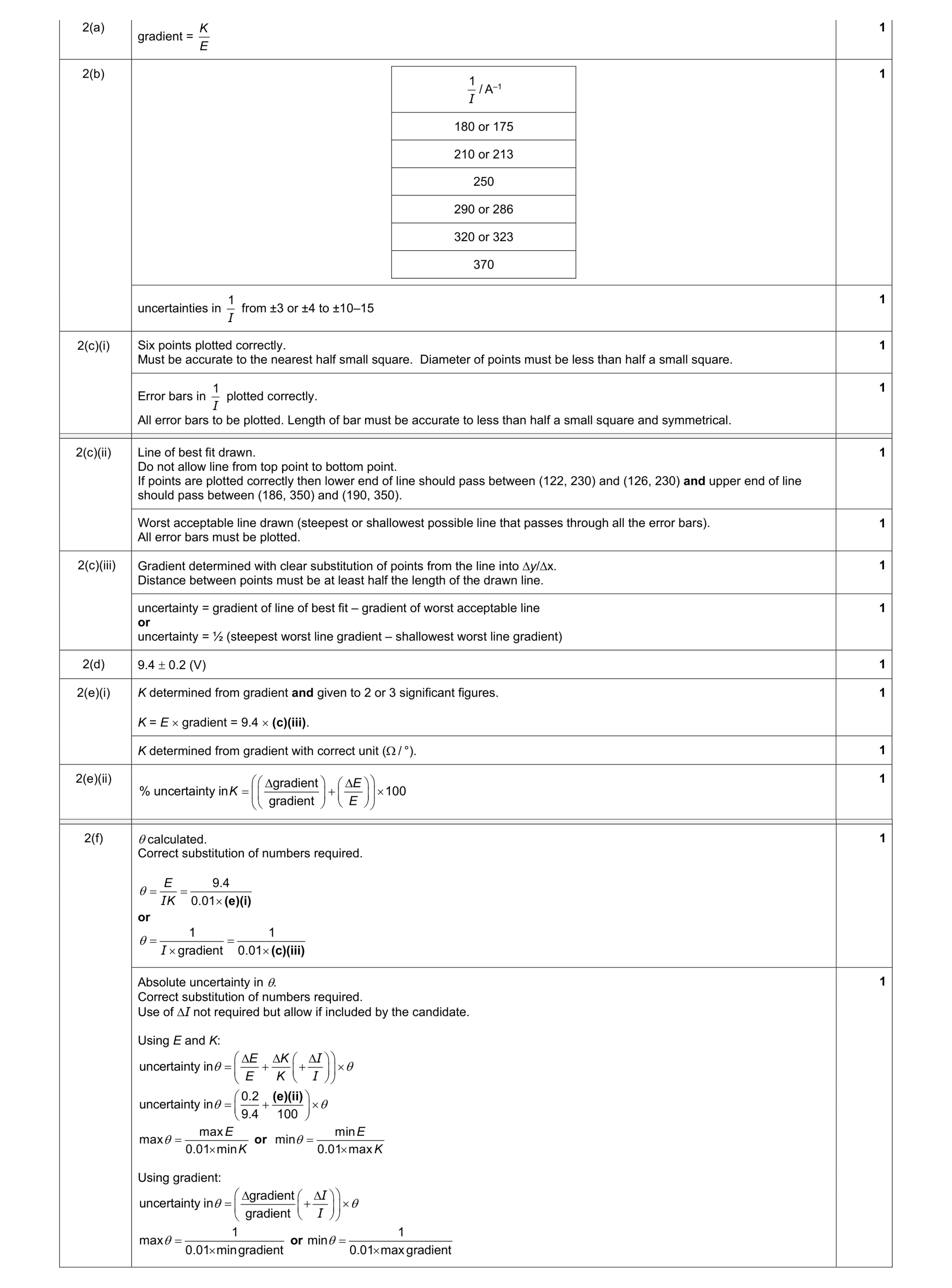 9
9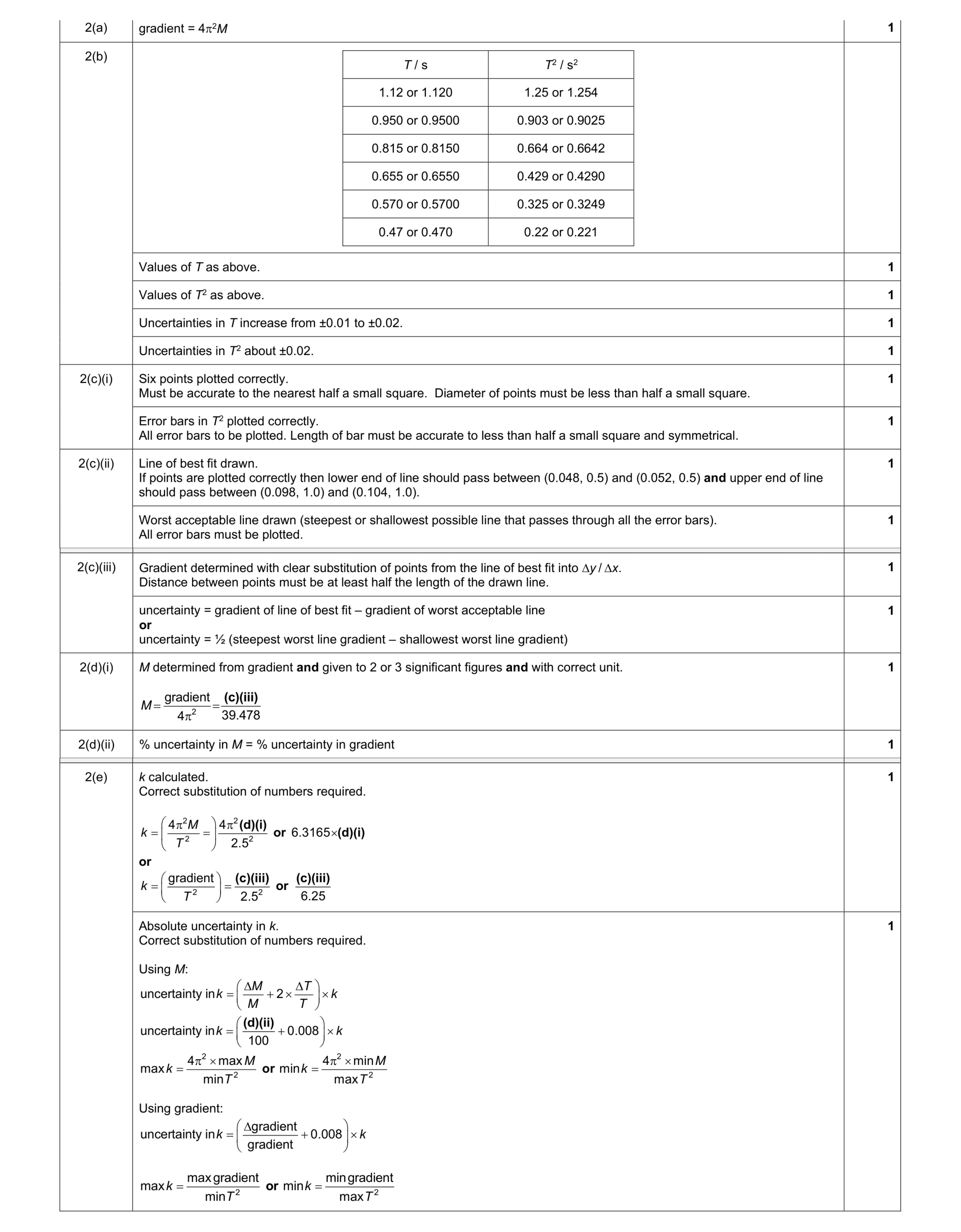 11
11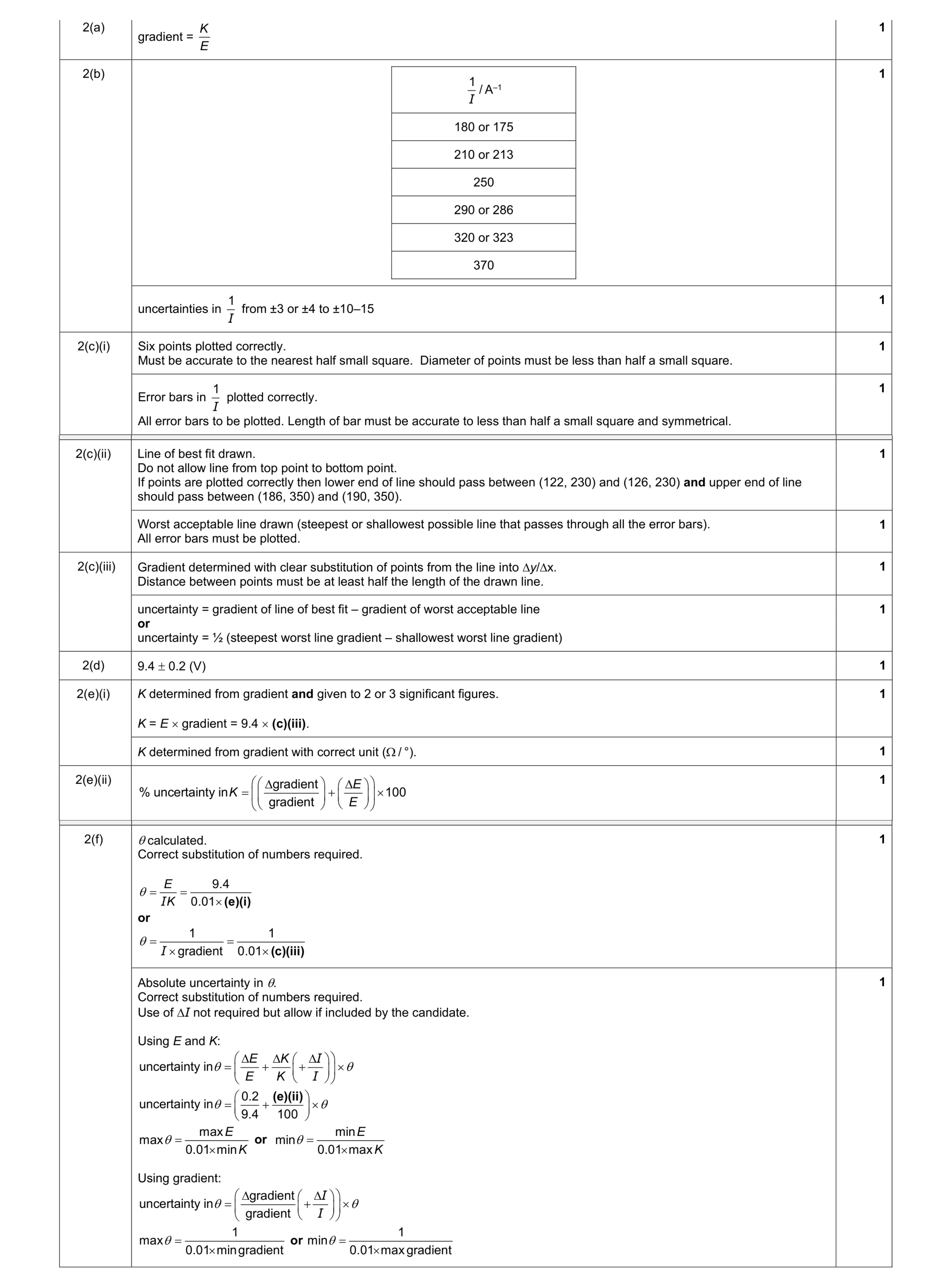 9
9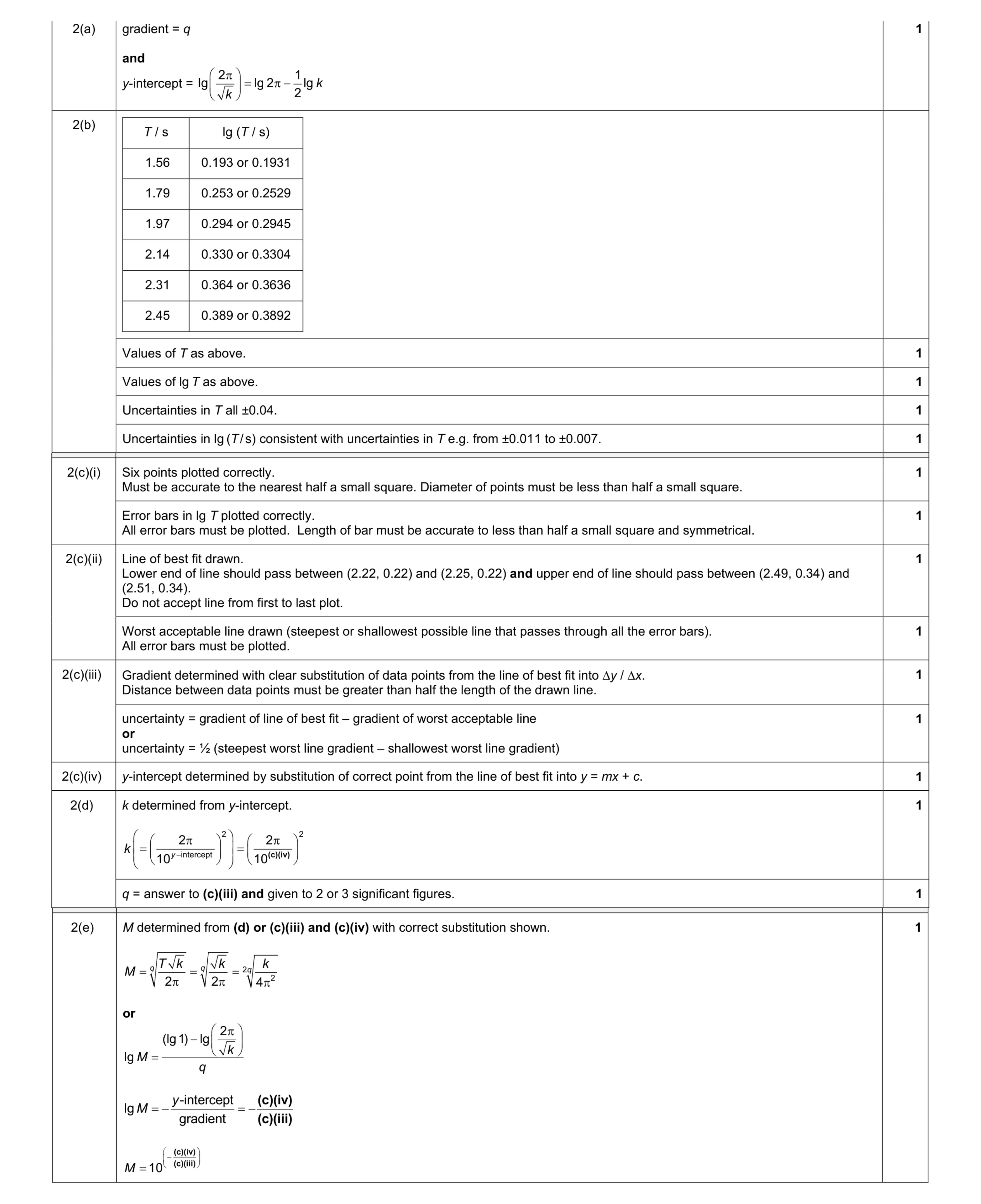 11
11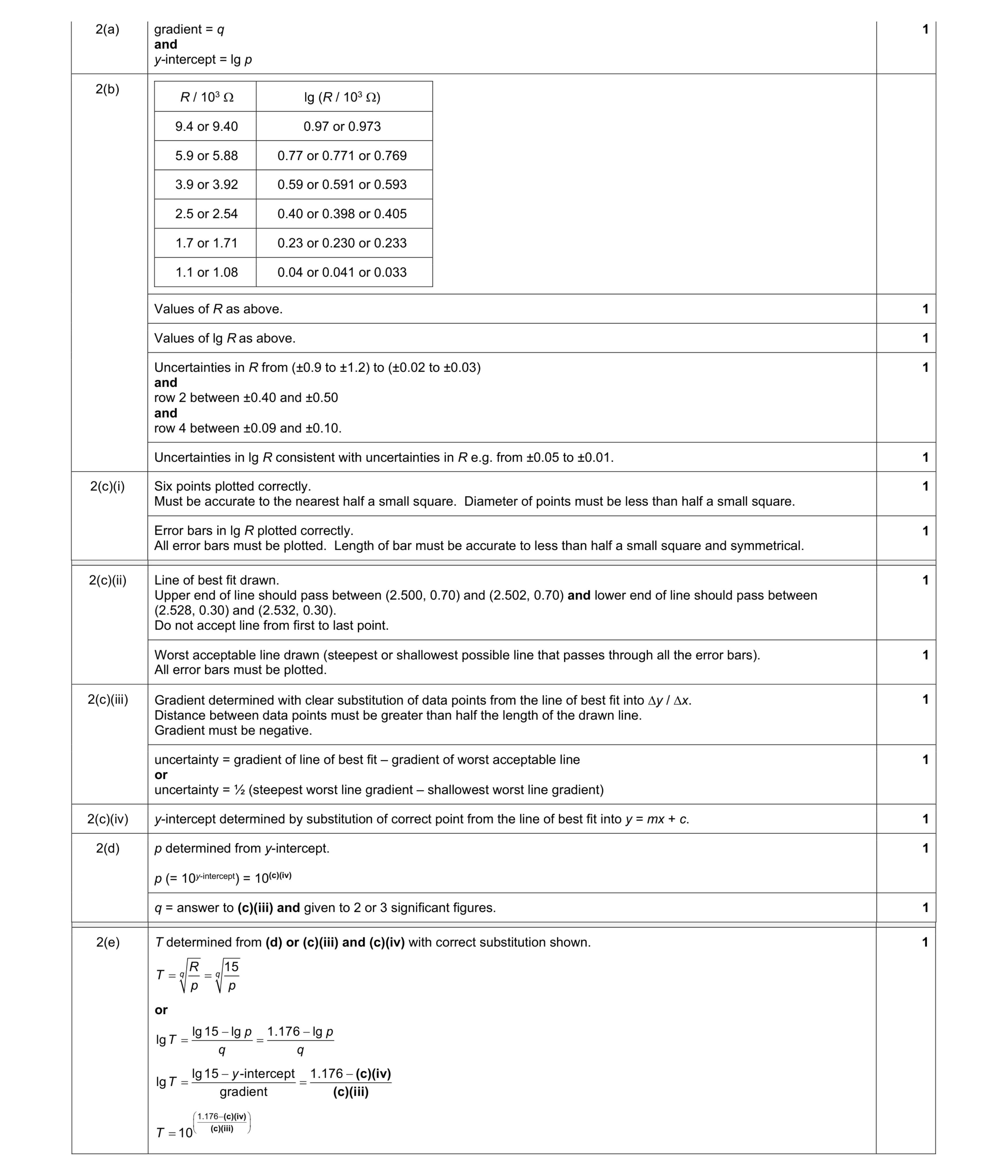 11
11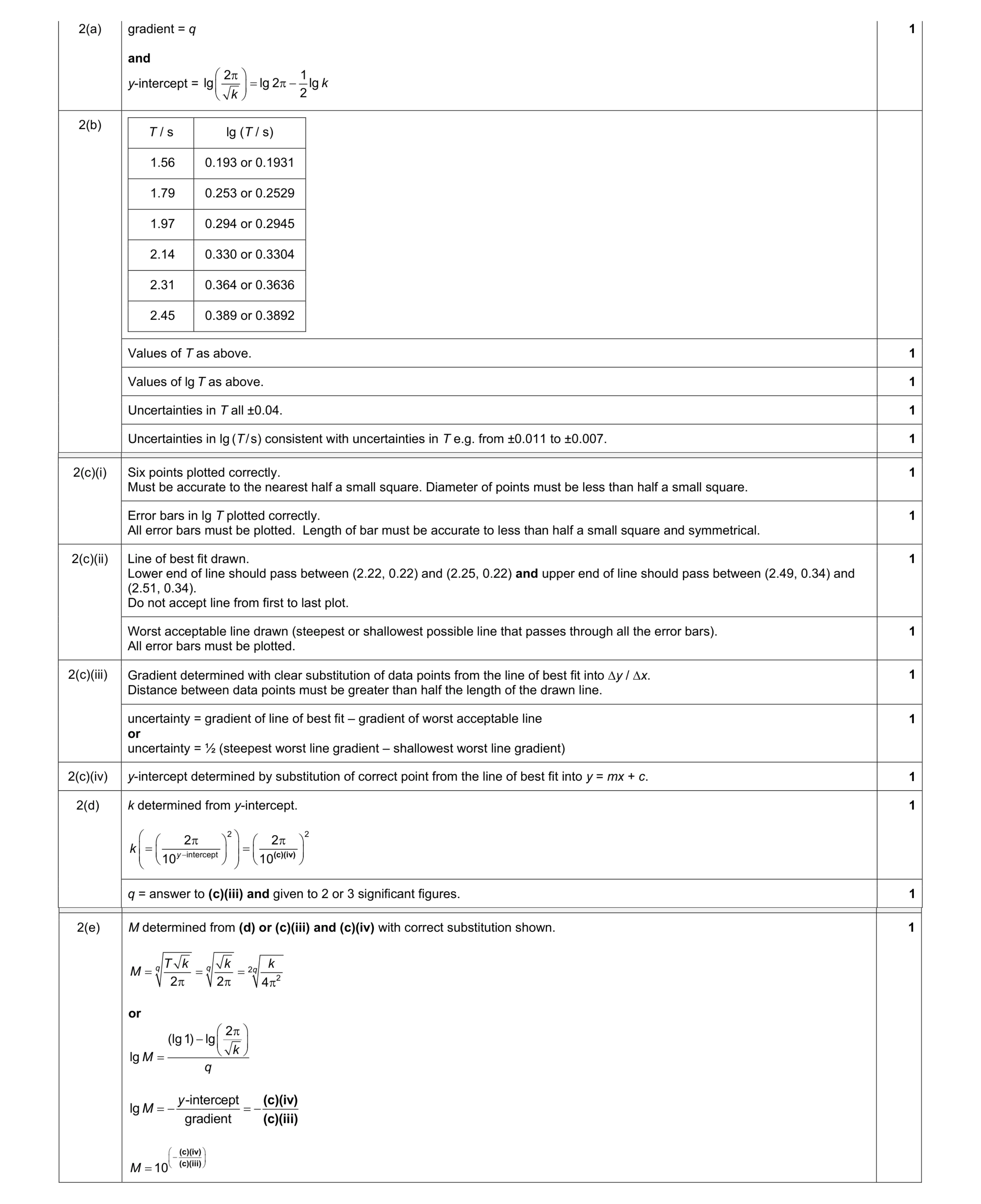 11
11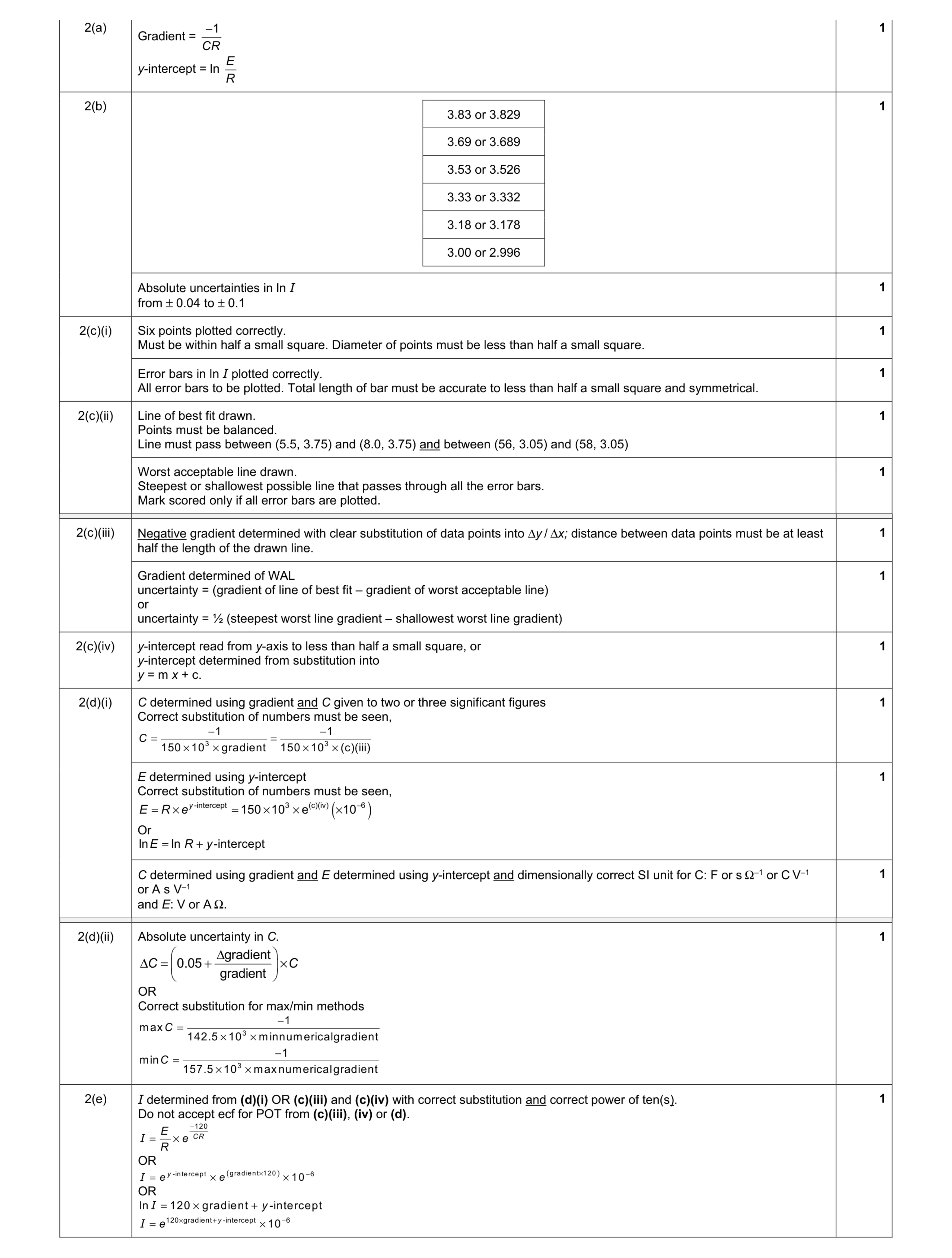 9
9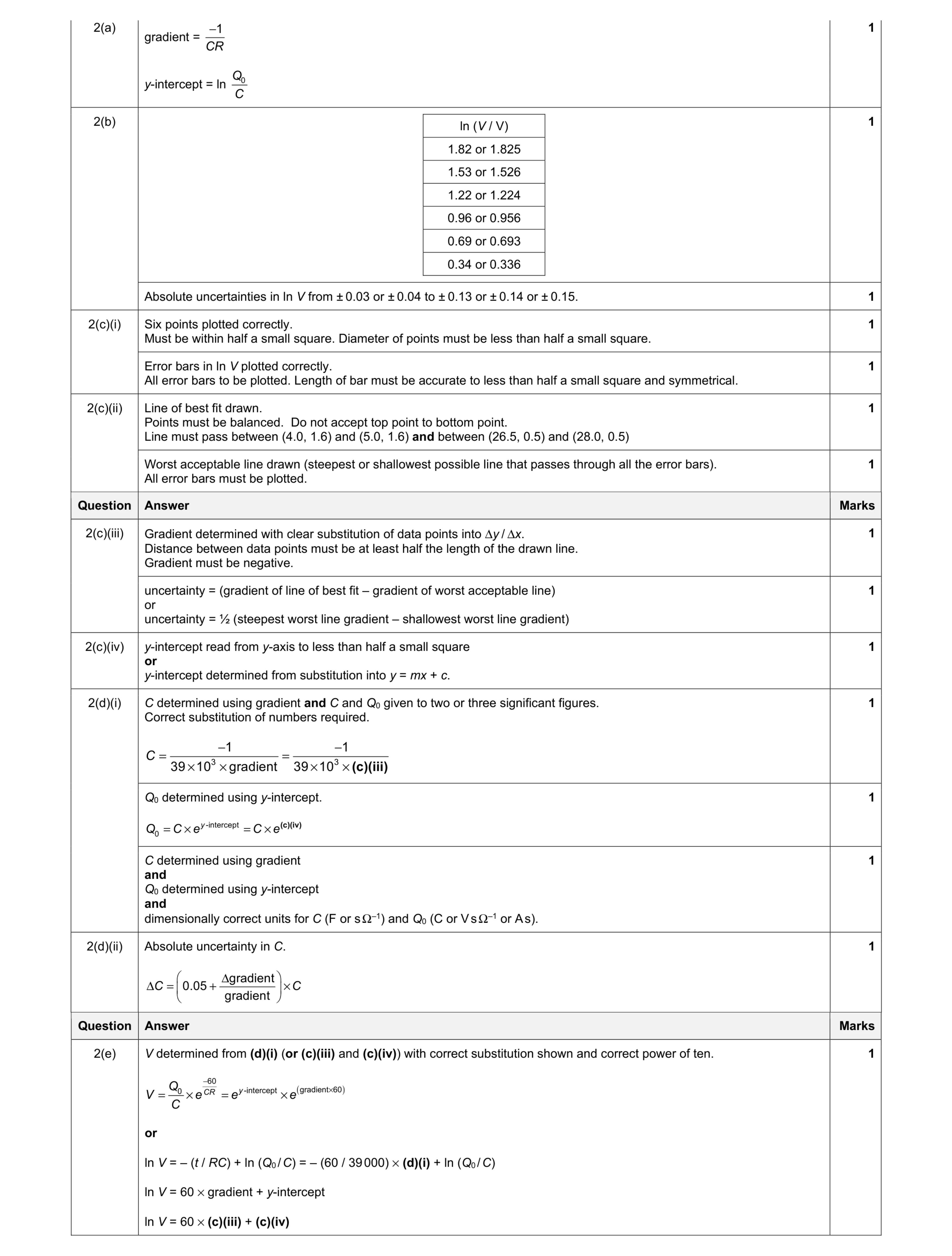 9
9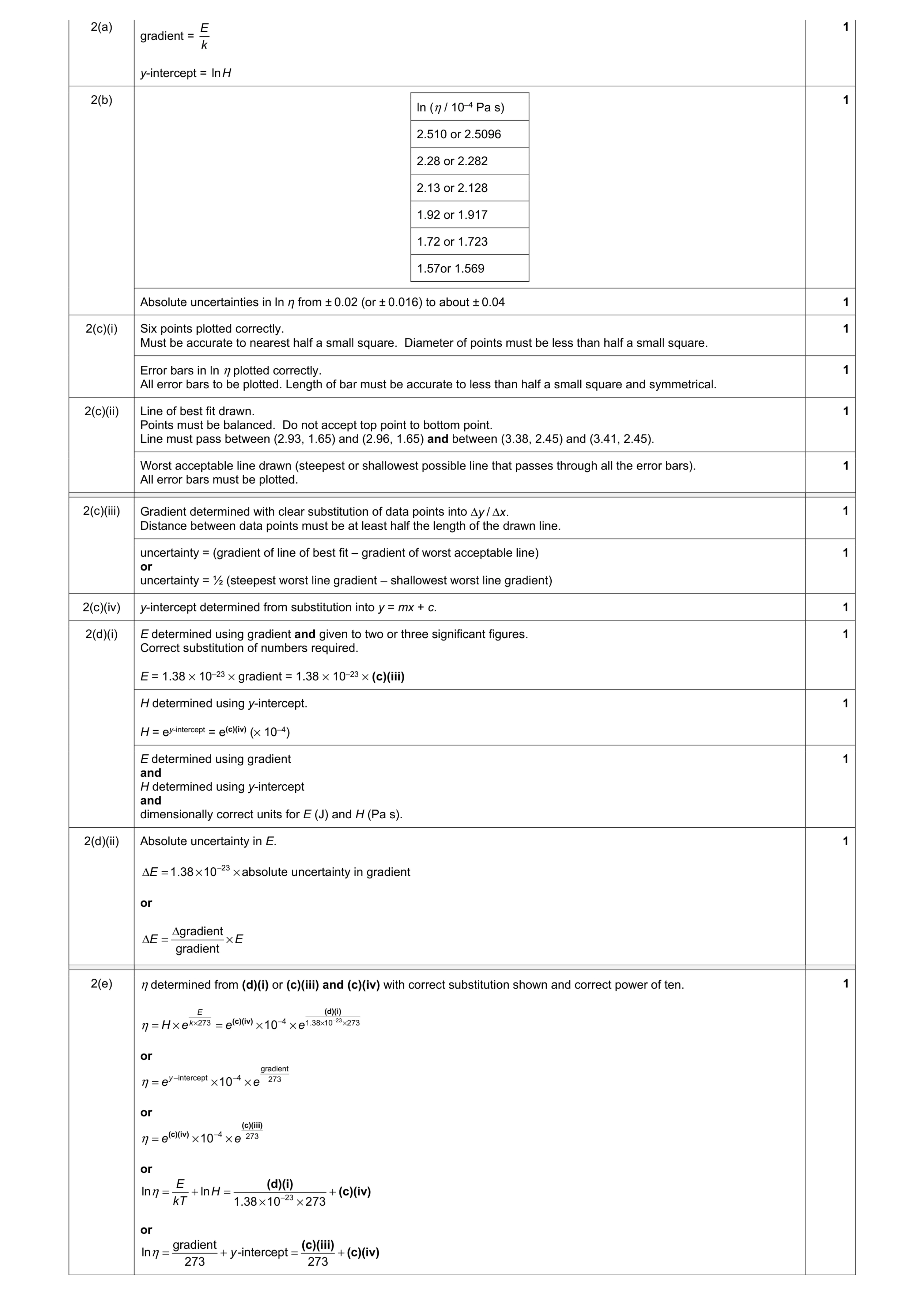 9
9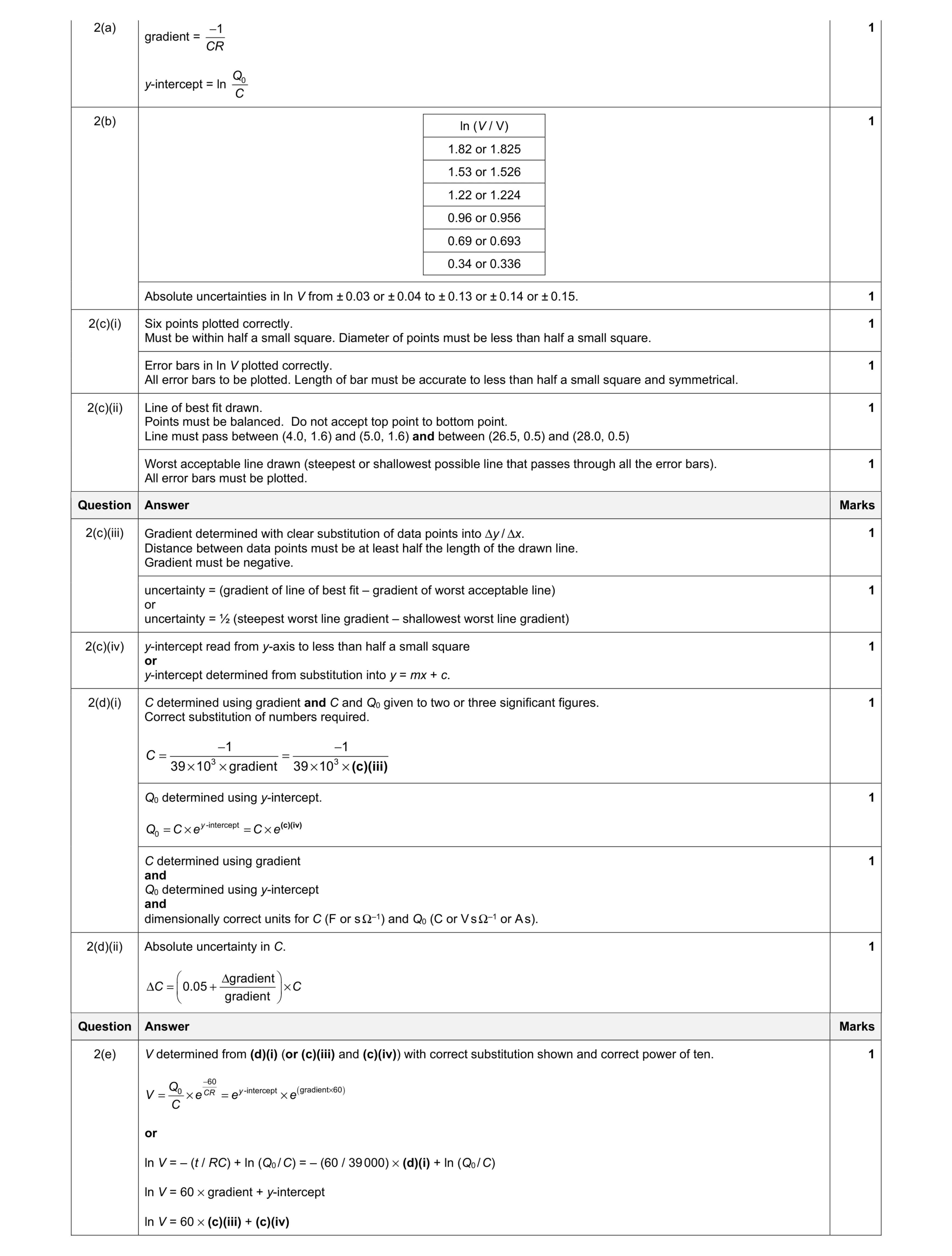 9
9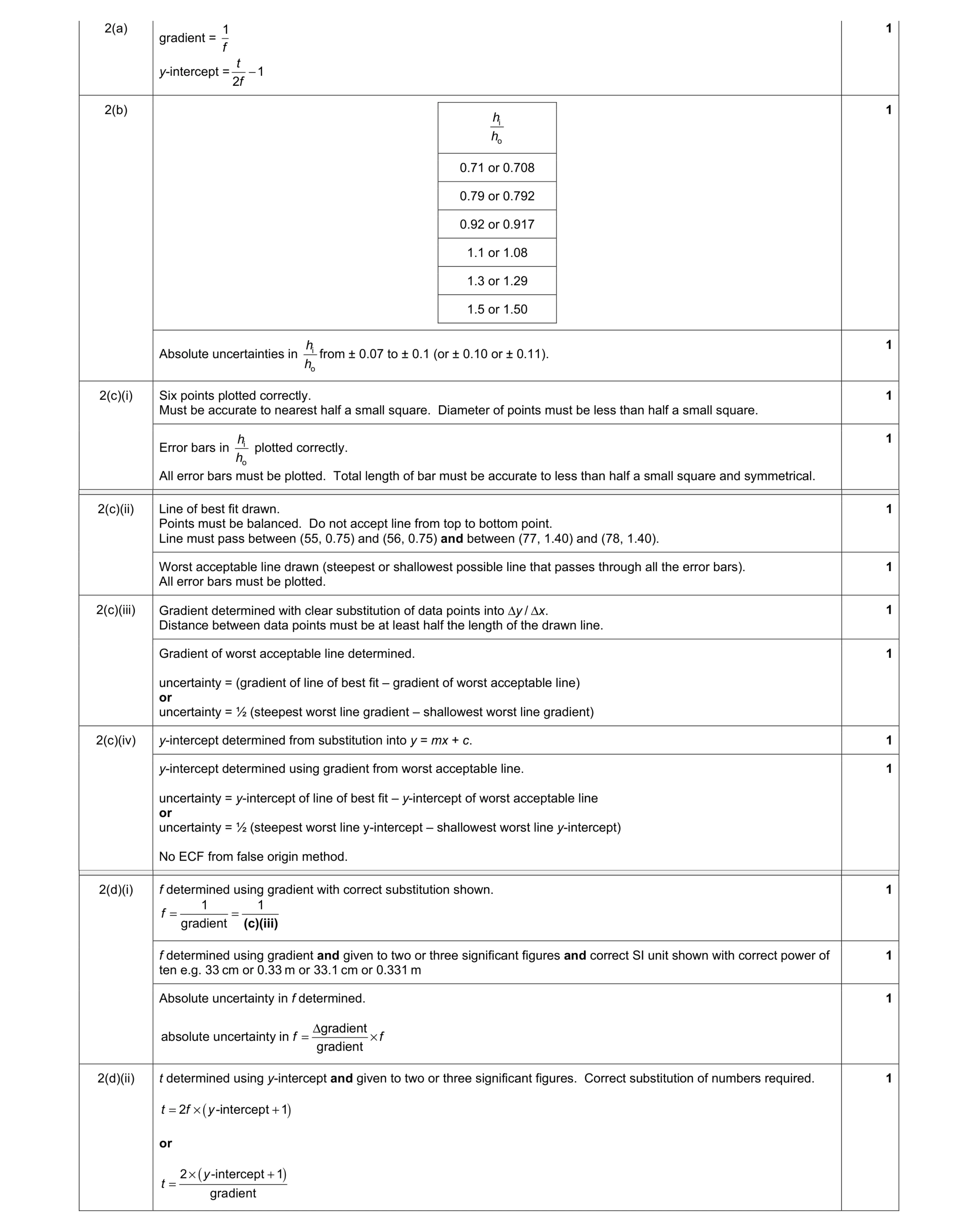 9
9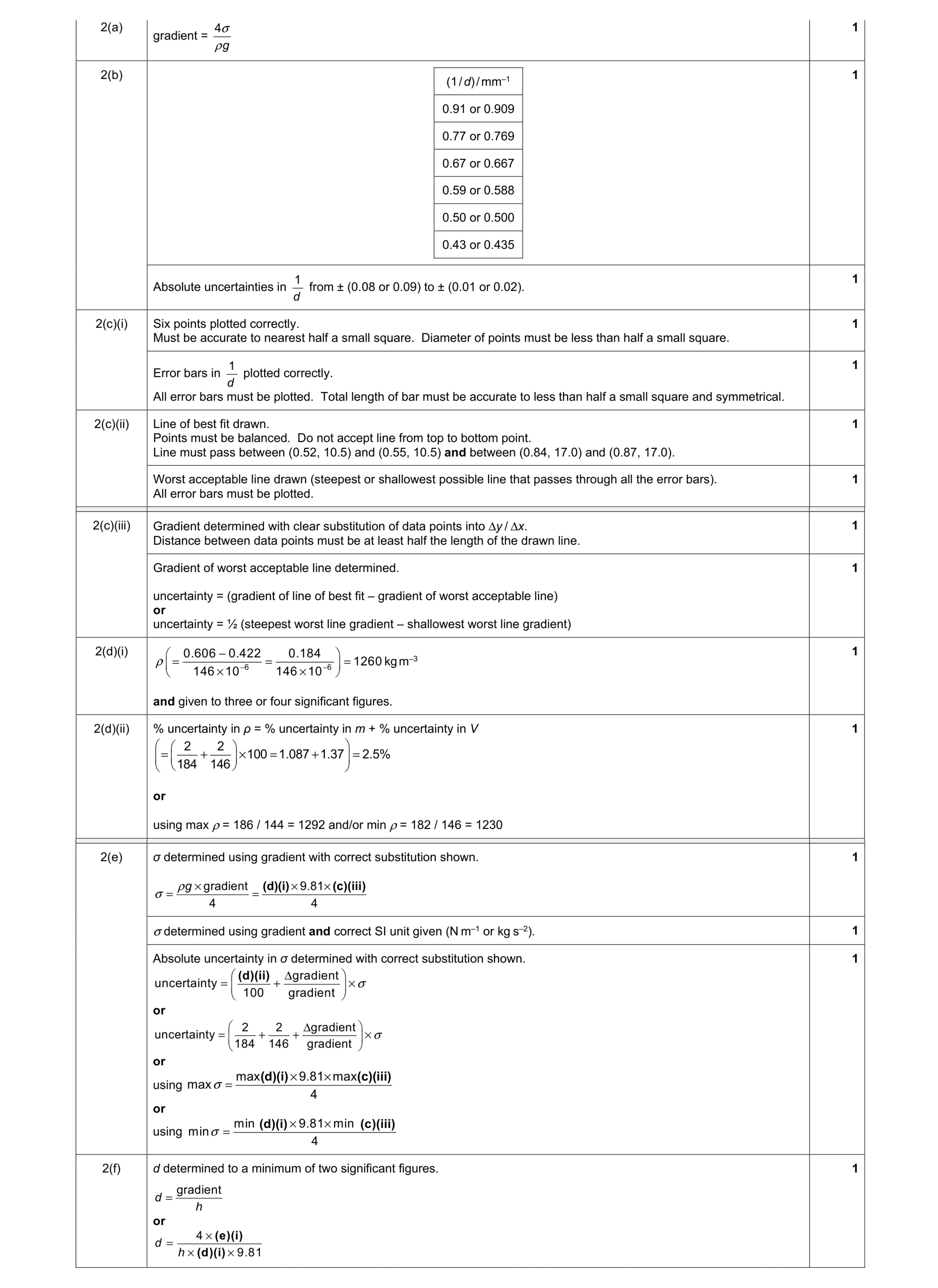 9
9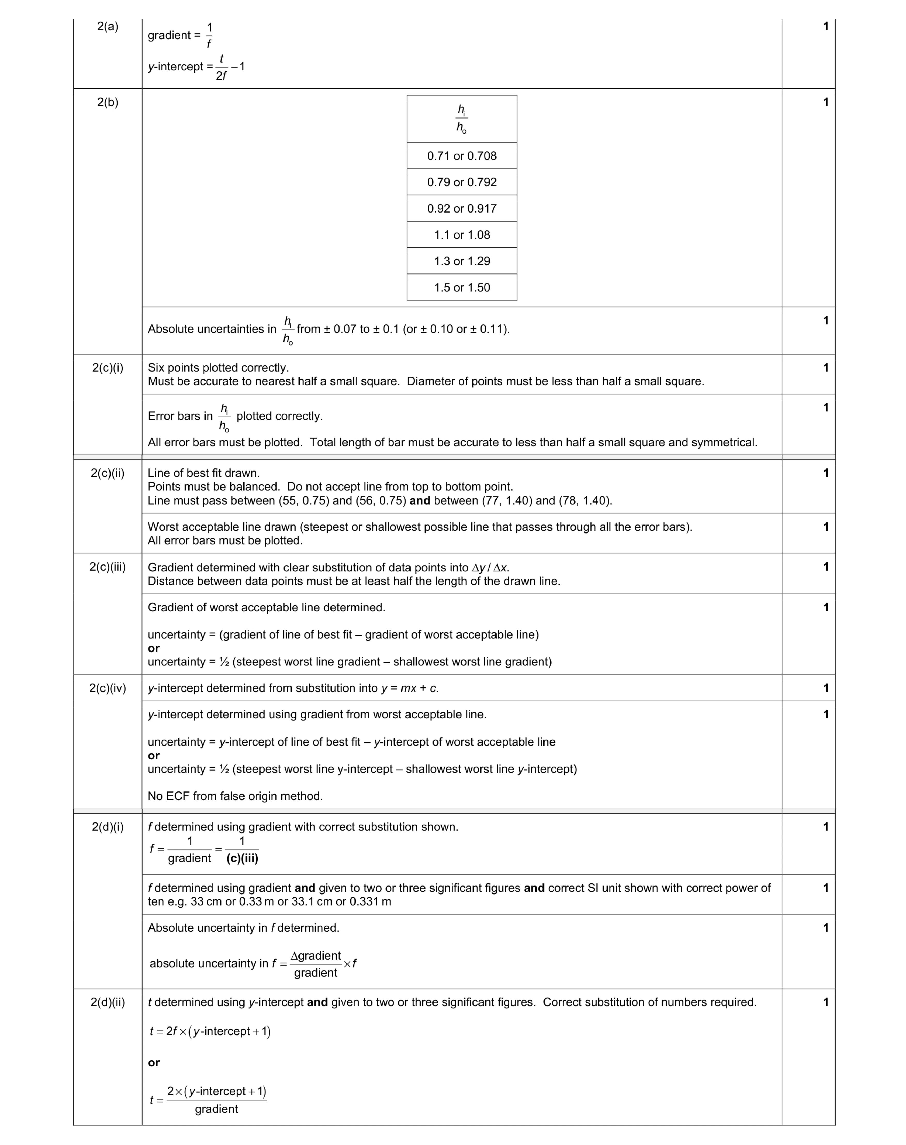 9
9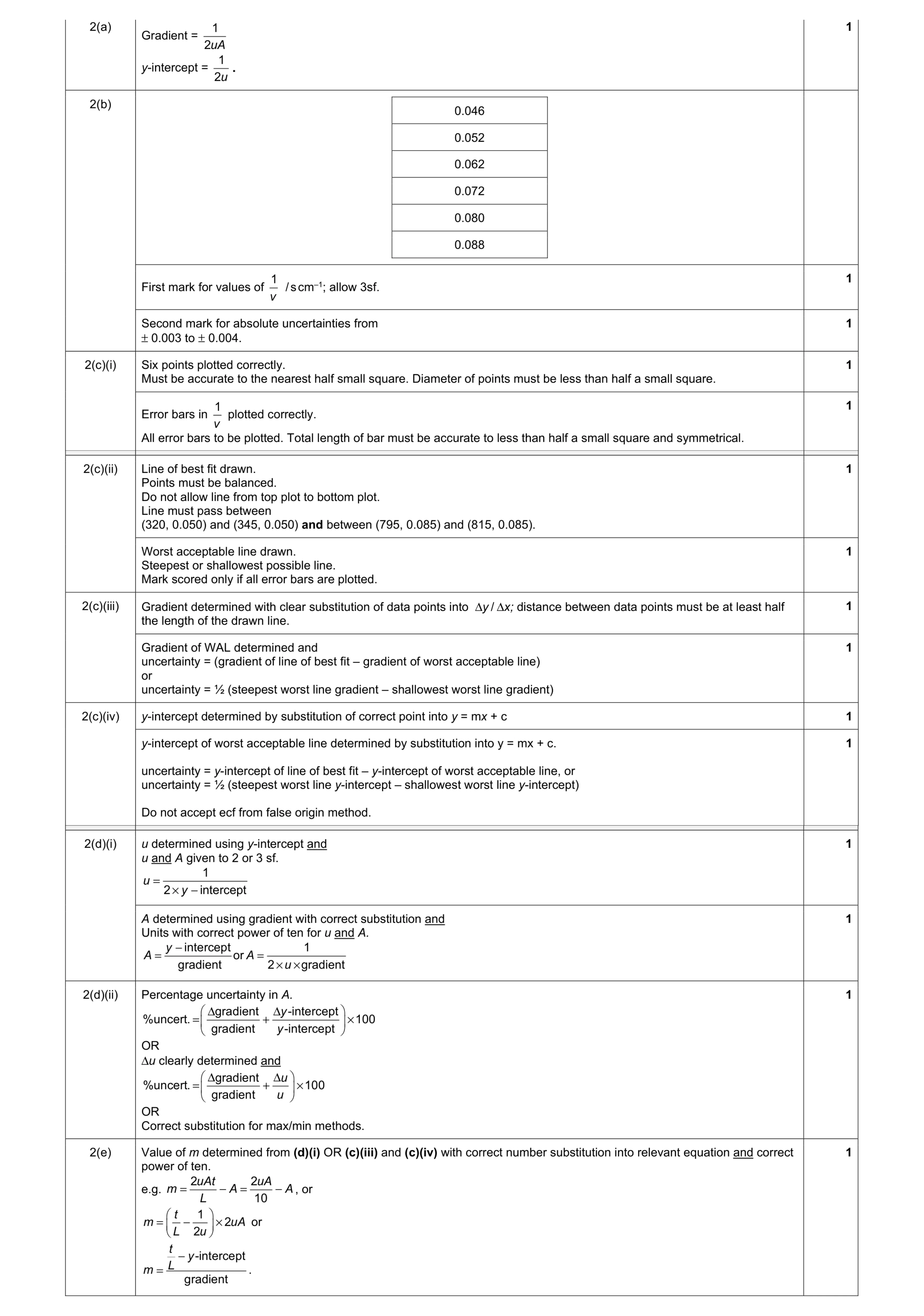 9
9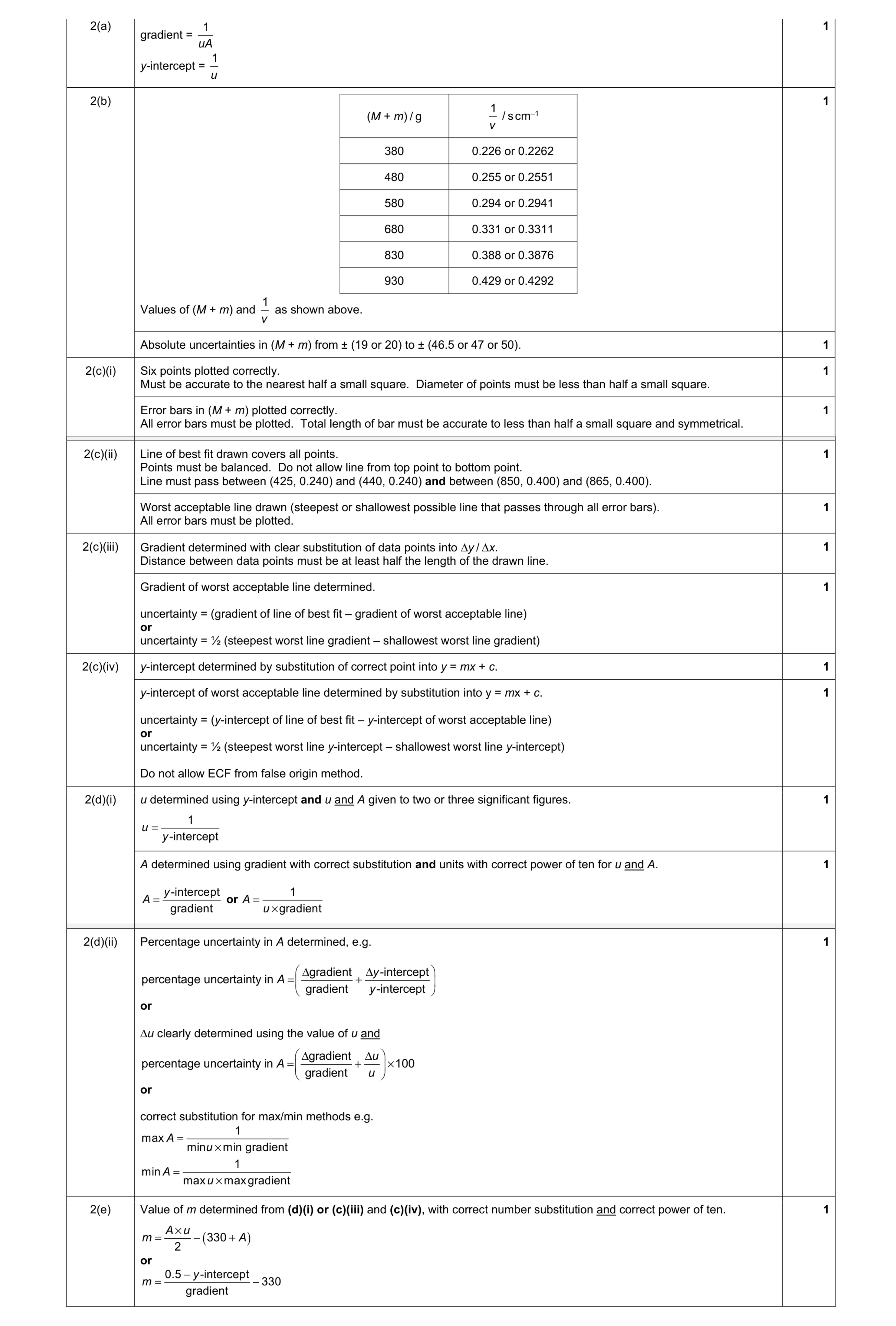 9
9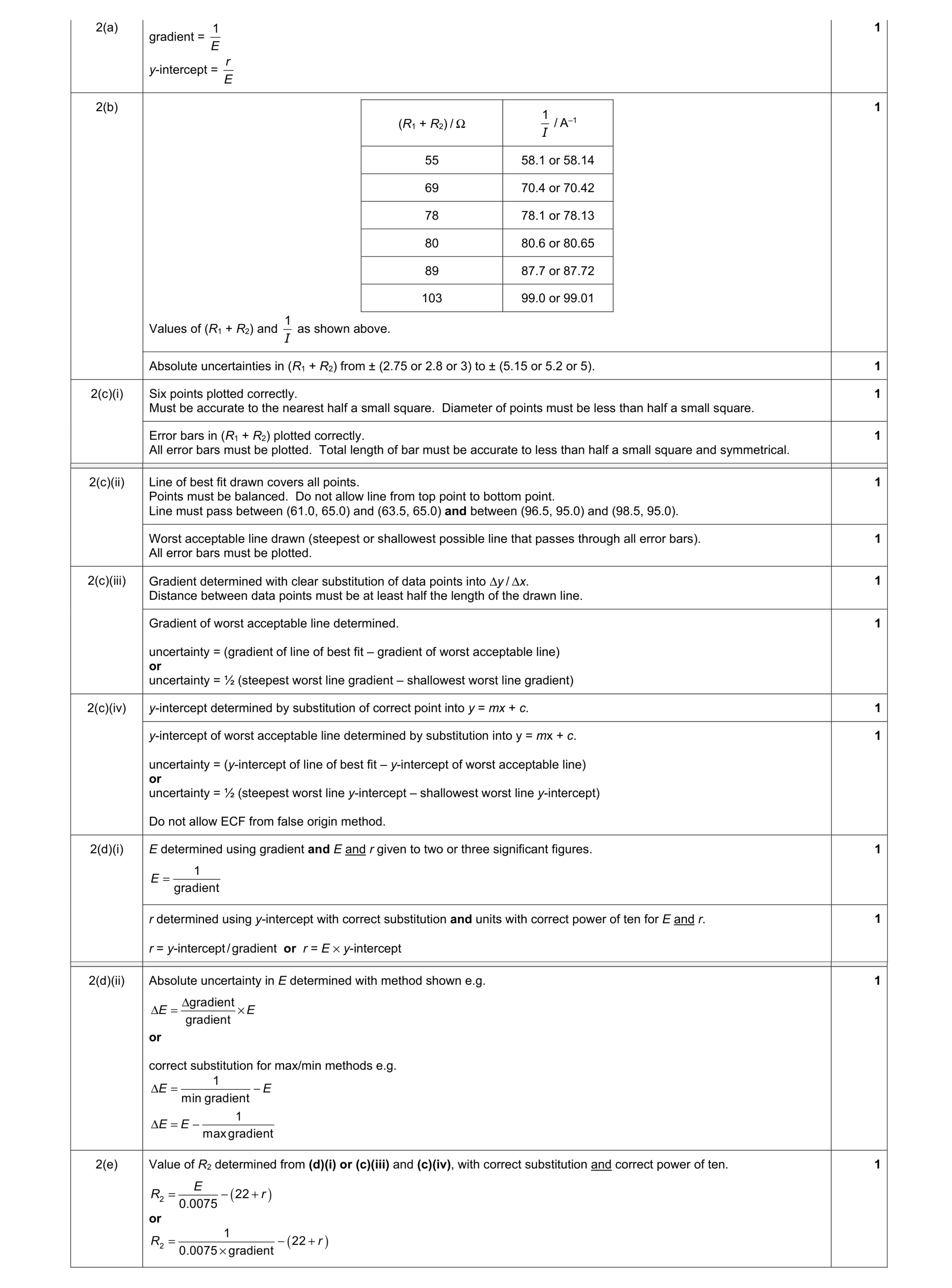 9
9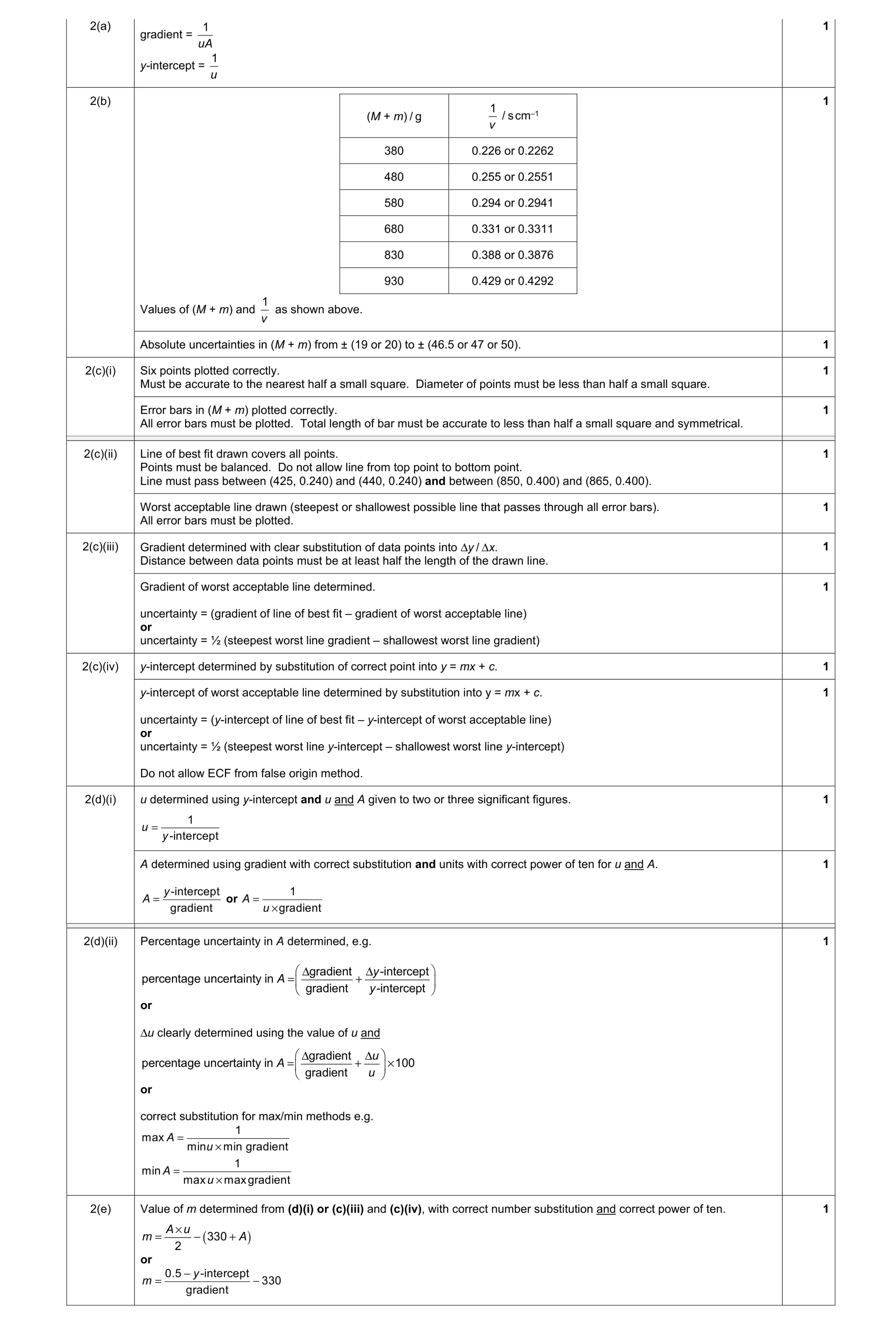 9
9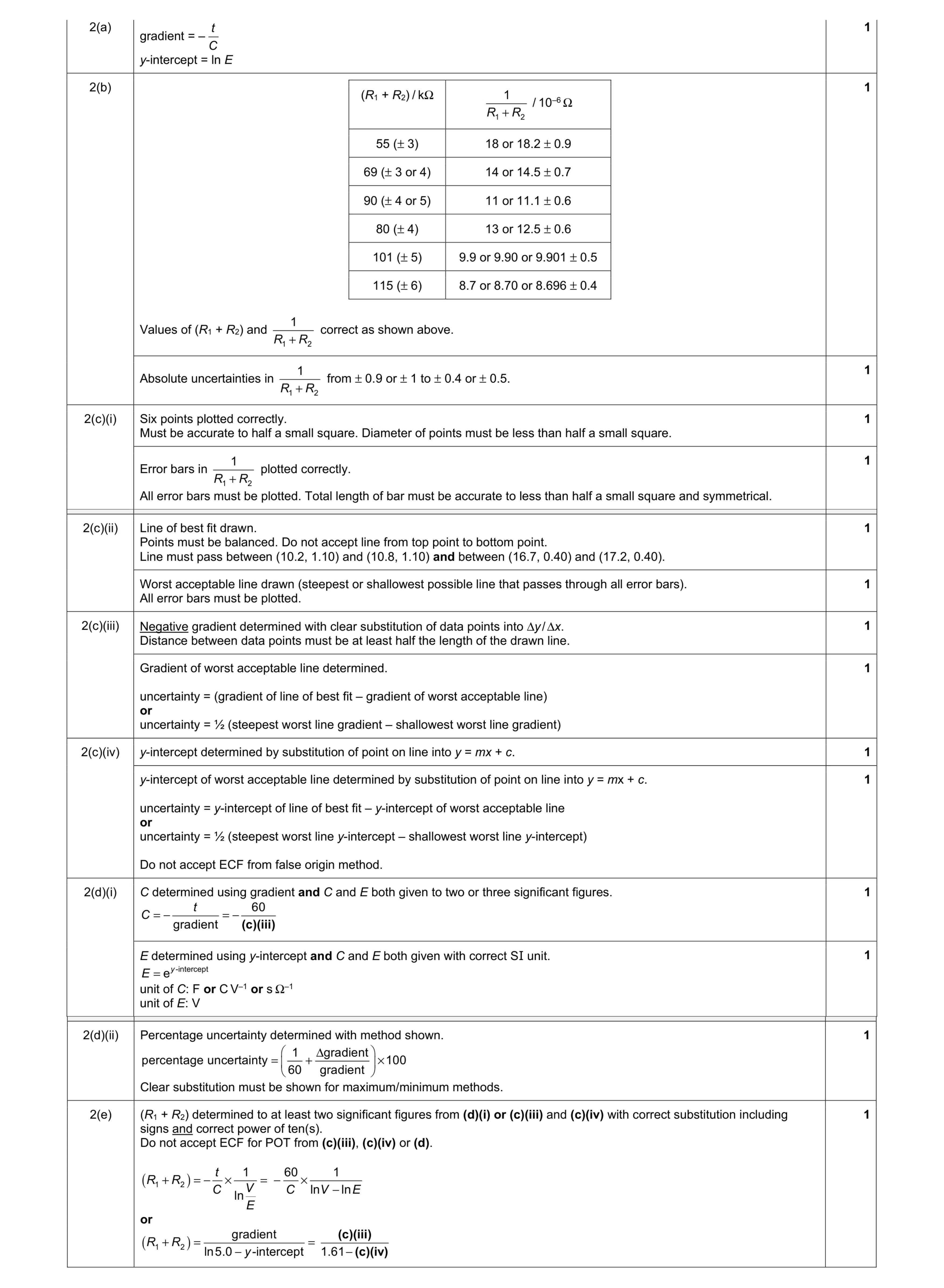 9
9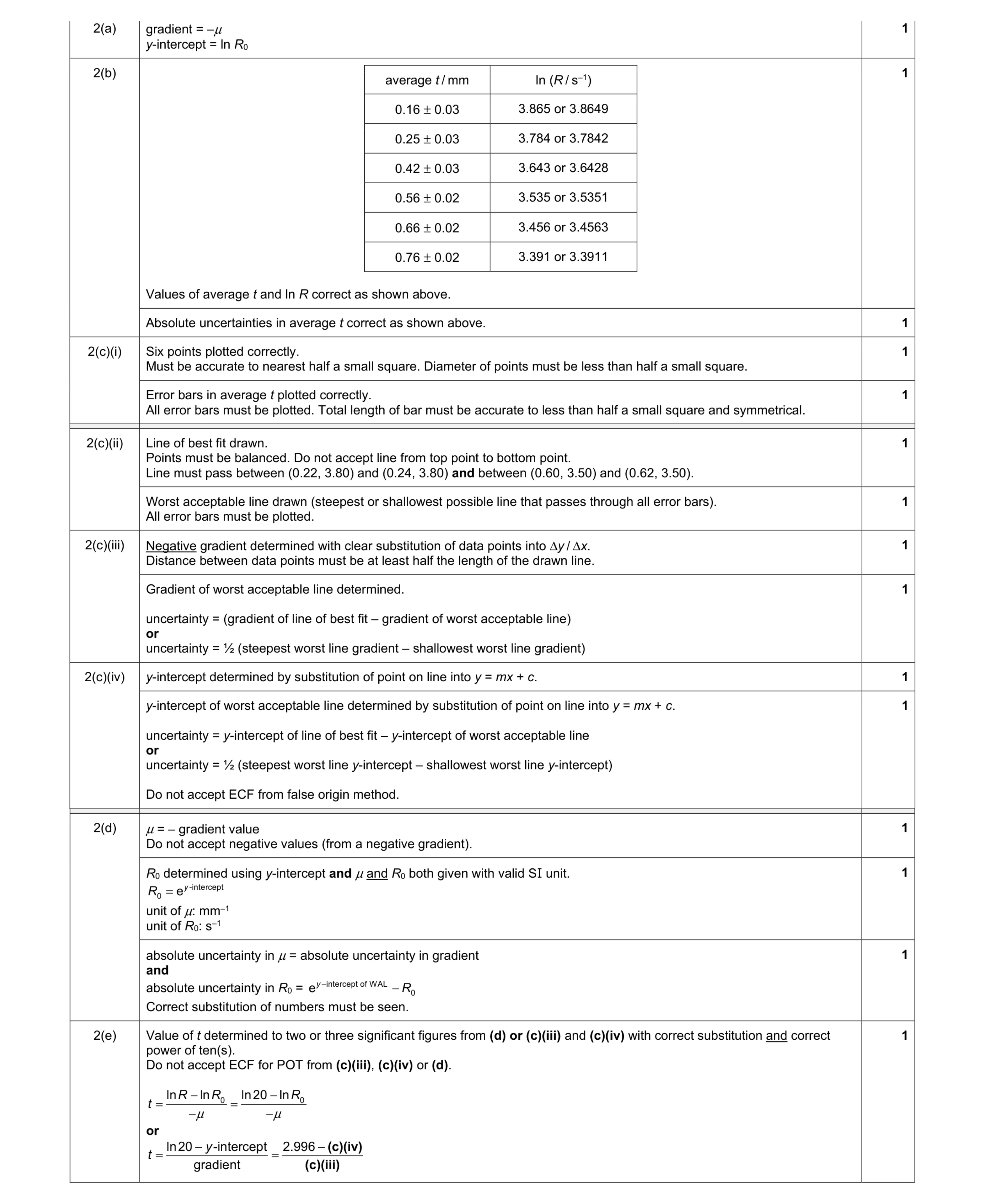 9
9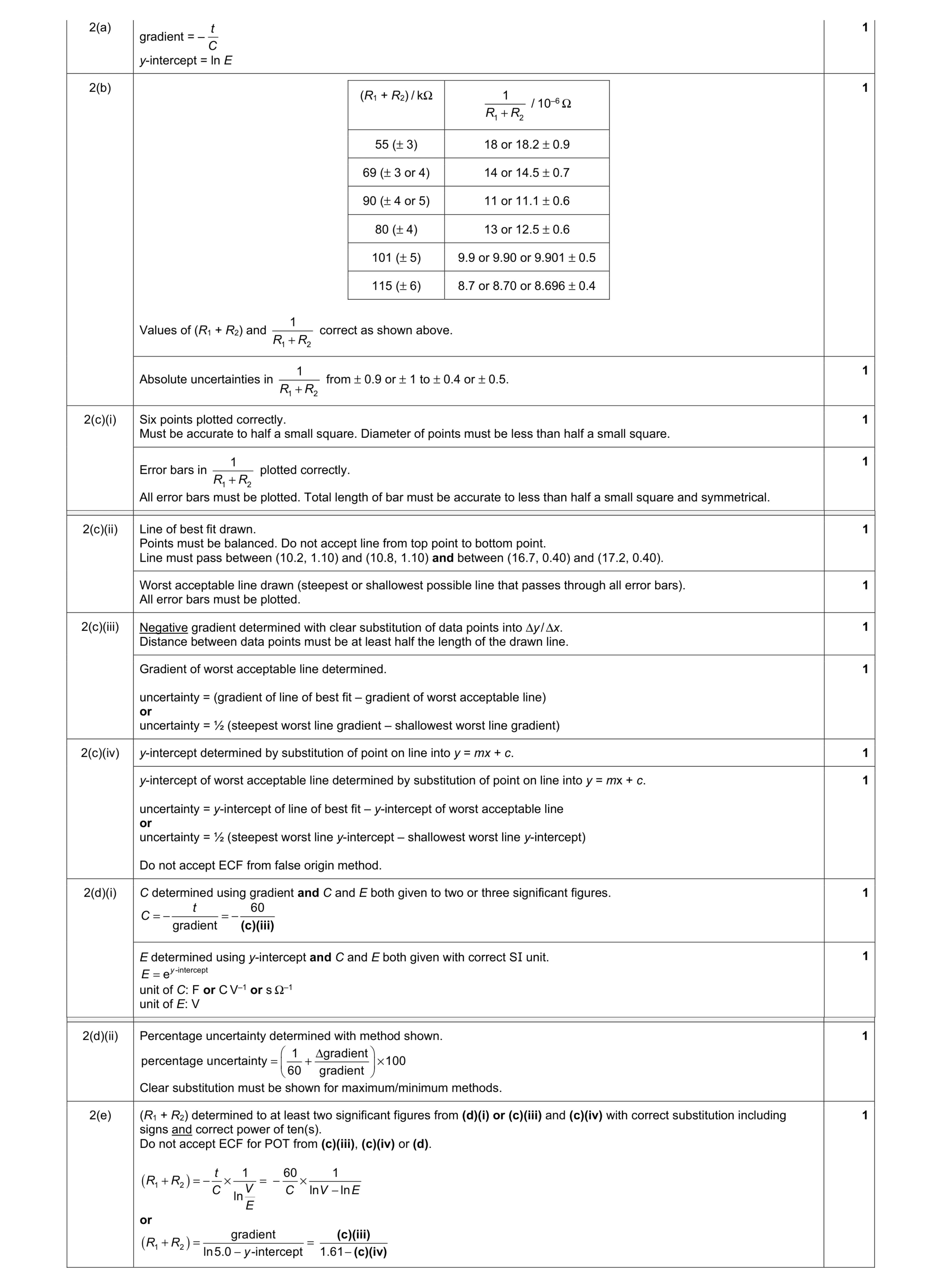 9
9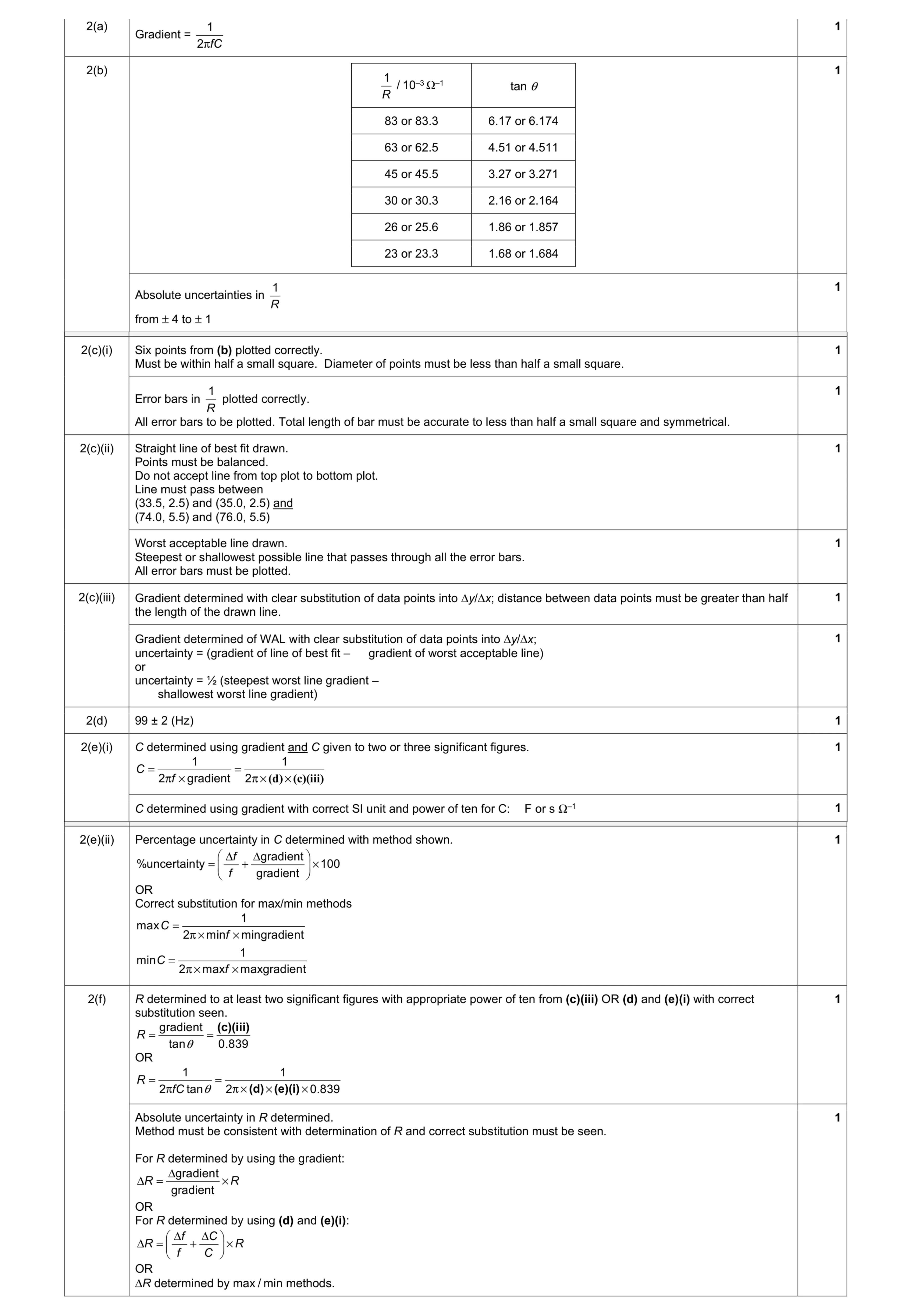 9
9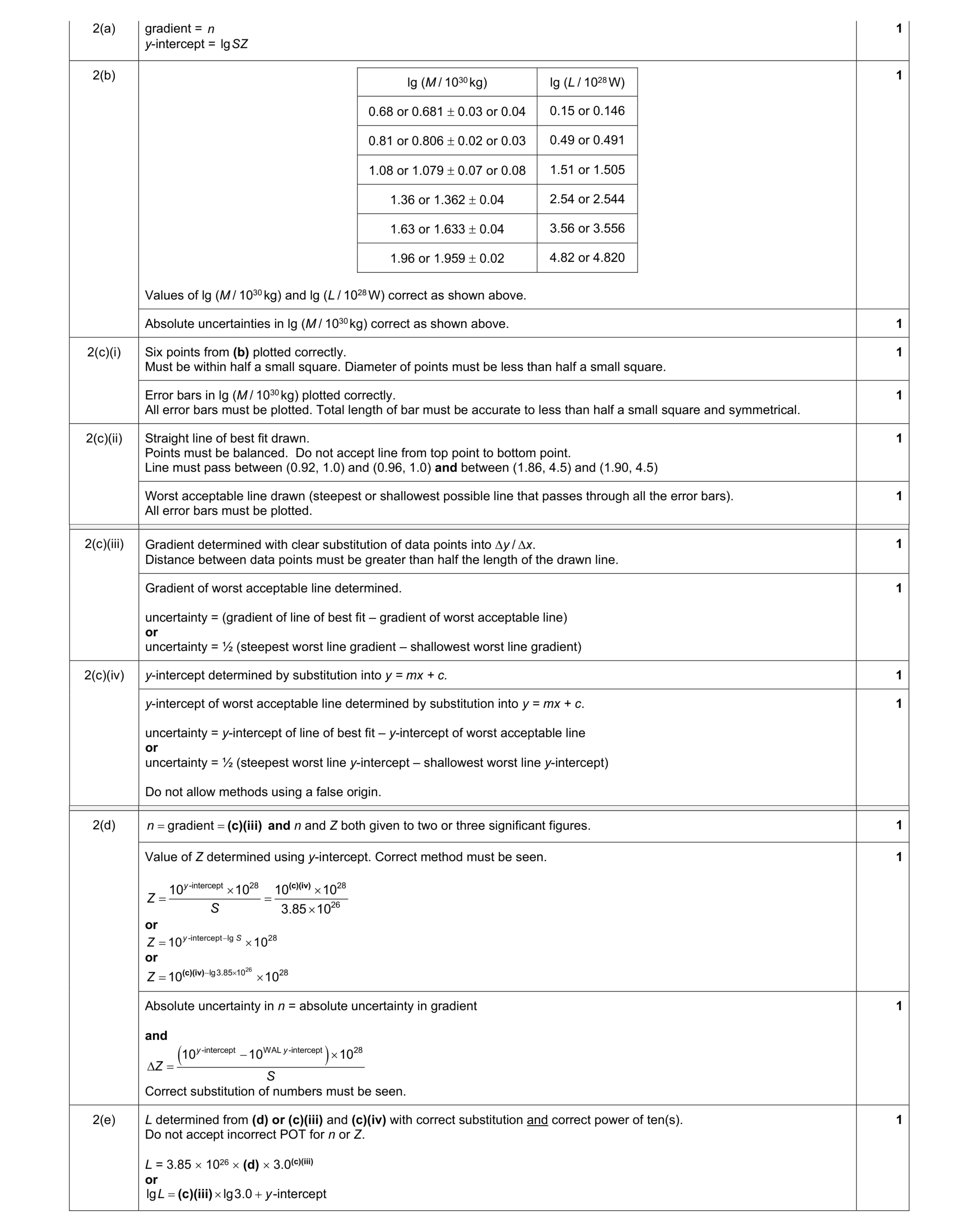 9
9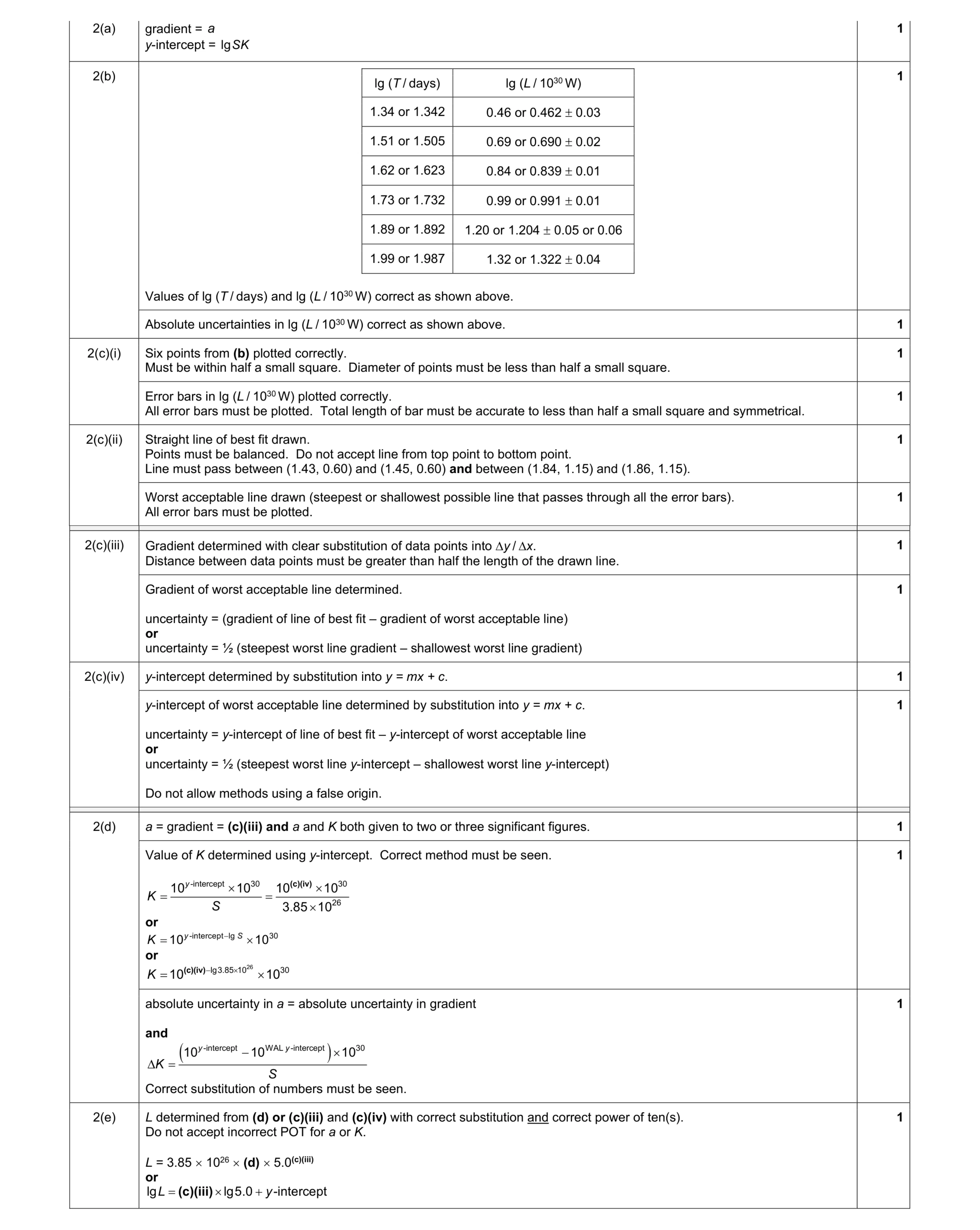 9
9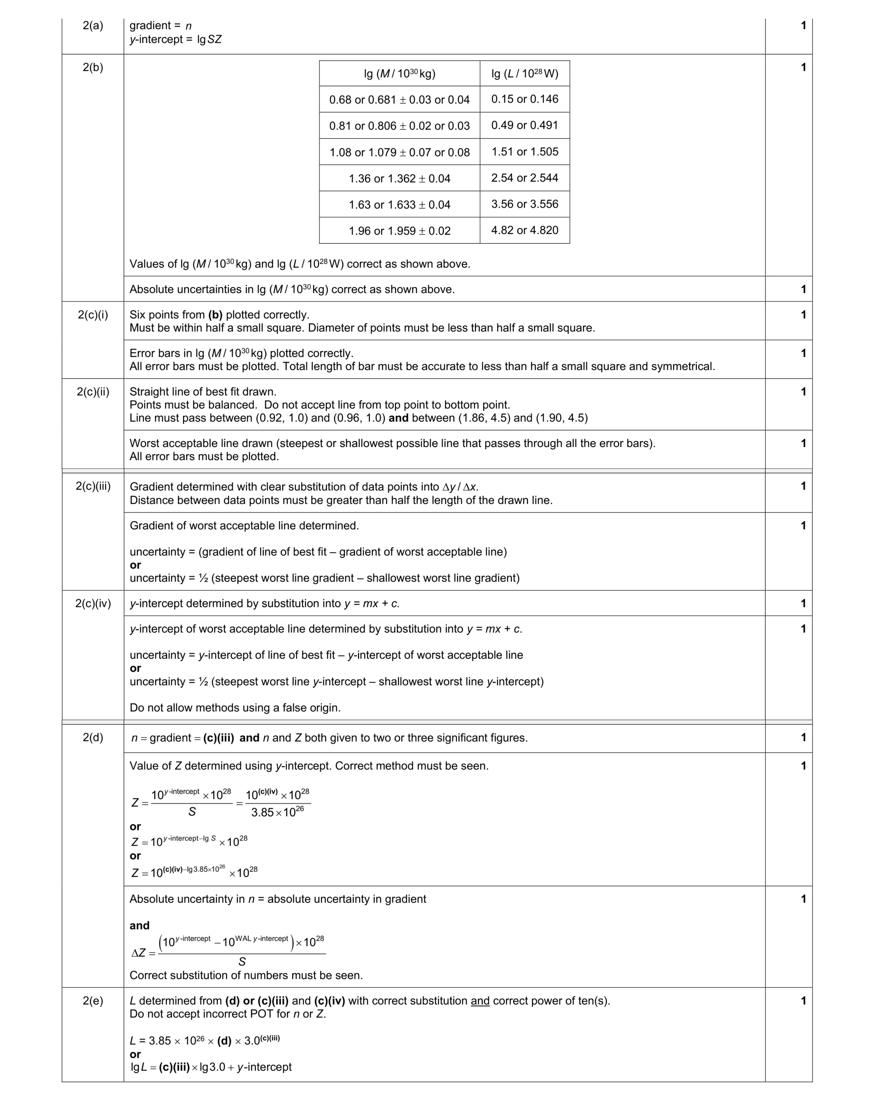 9
9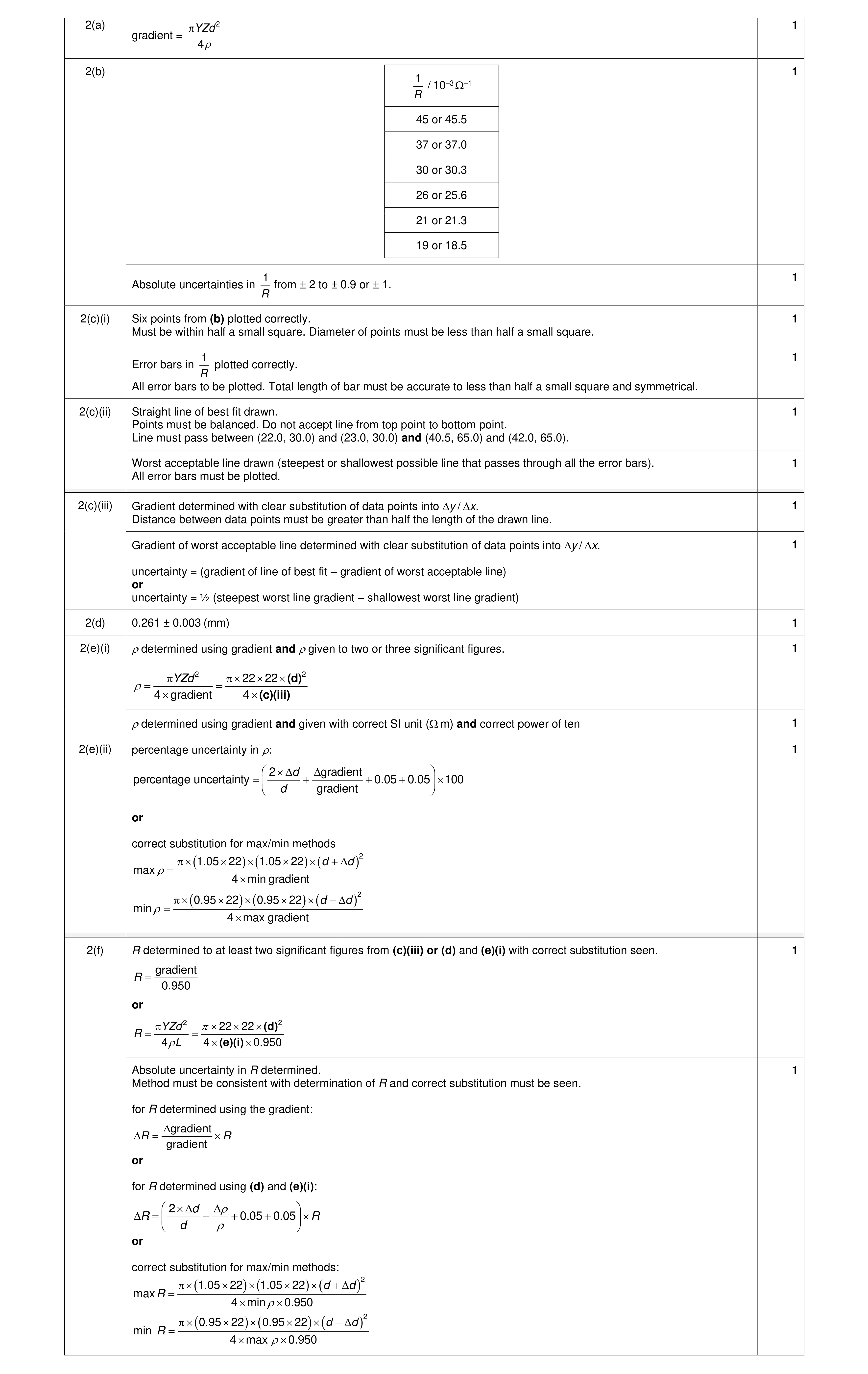 9
9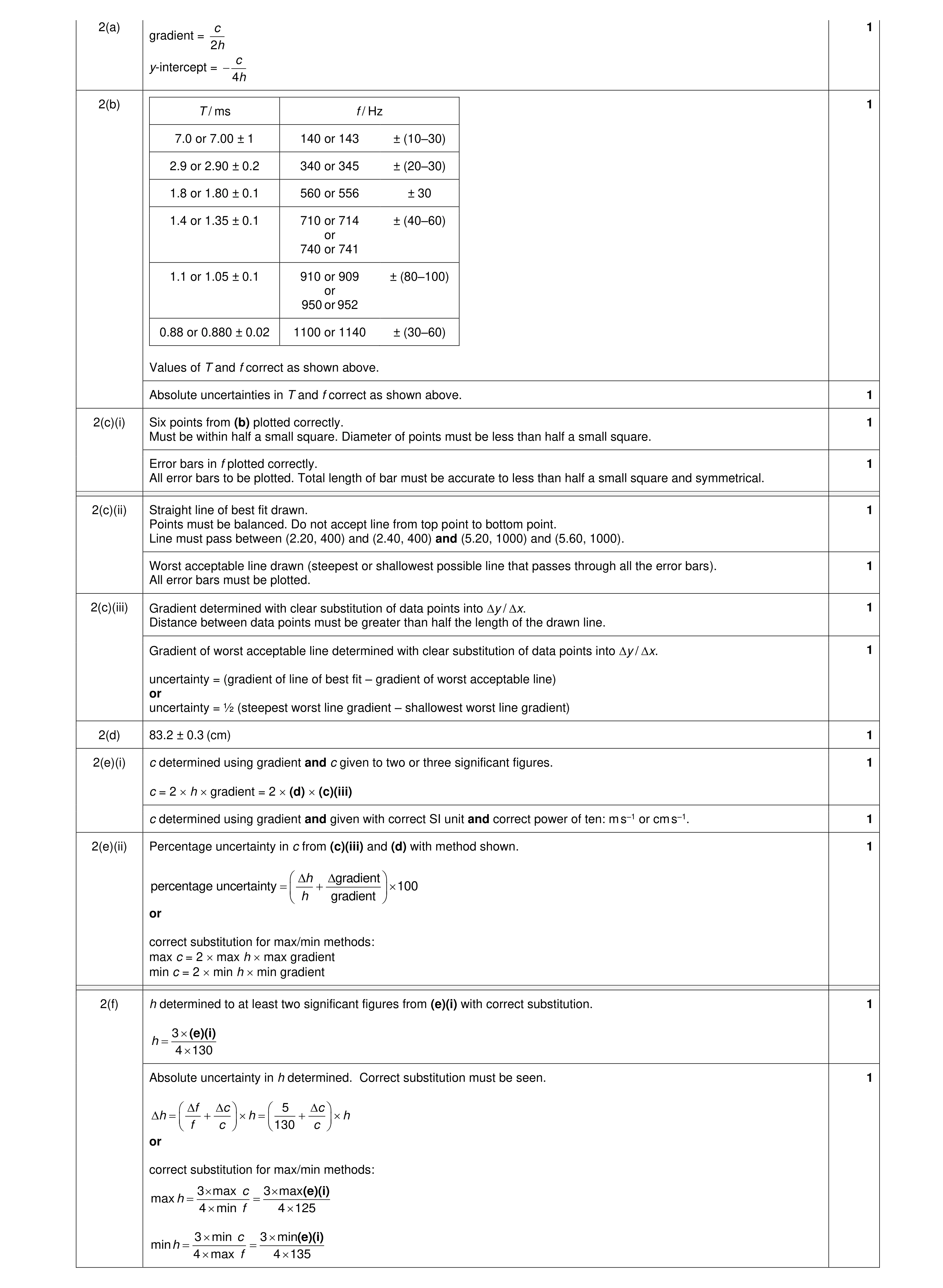 9
9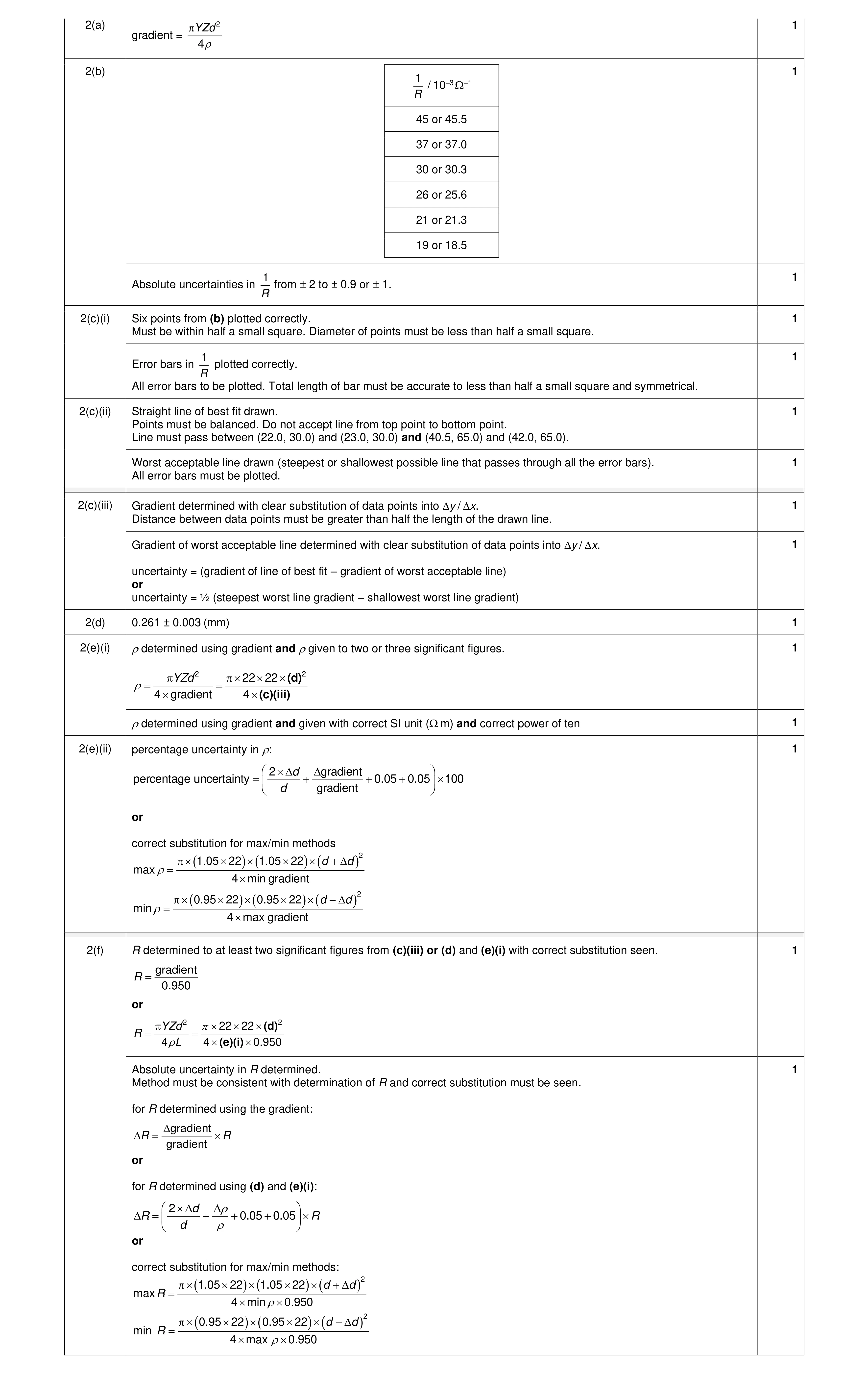 9
9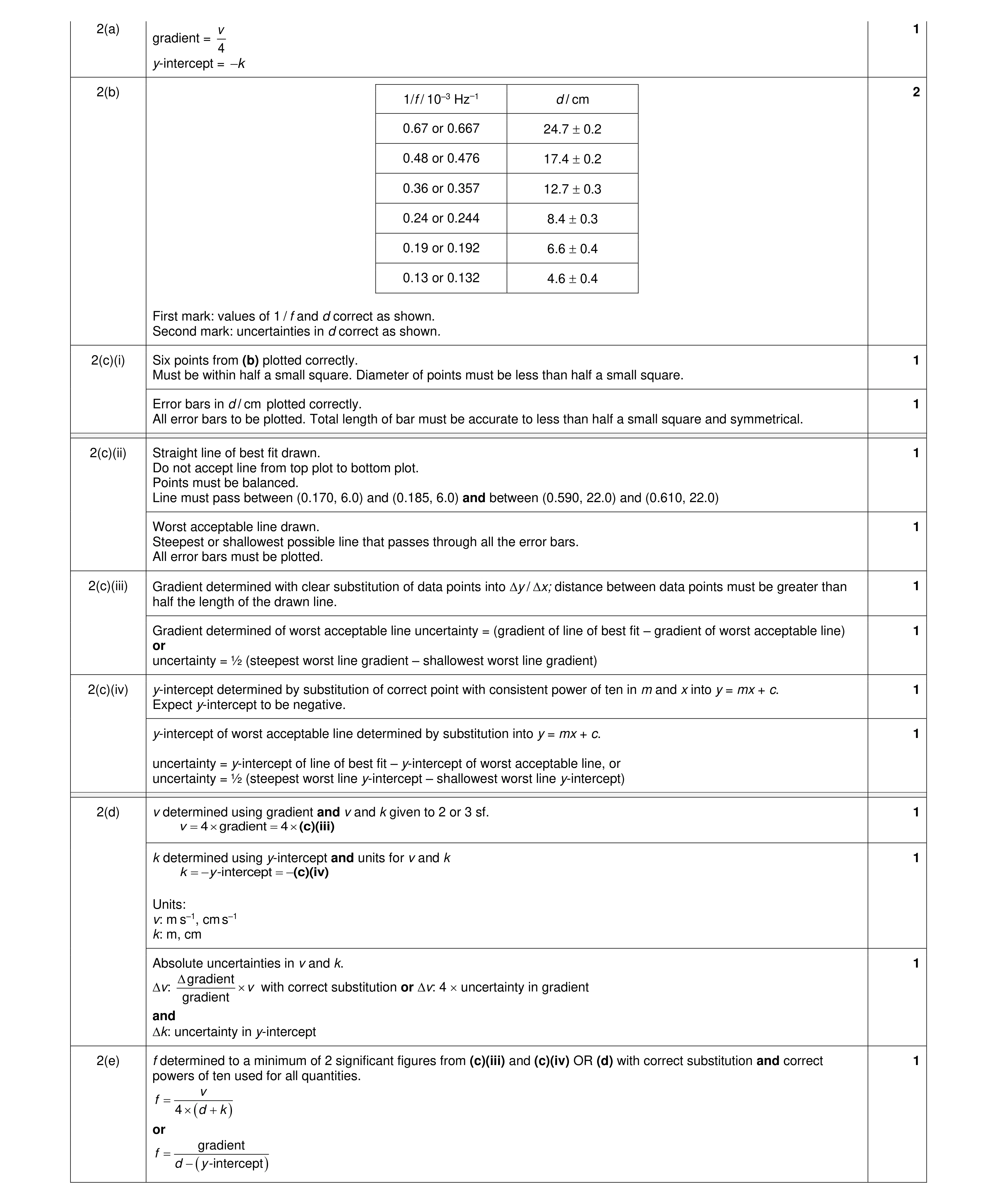 9
9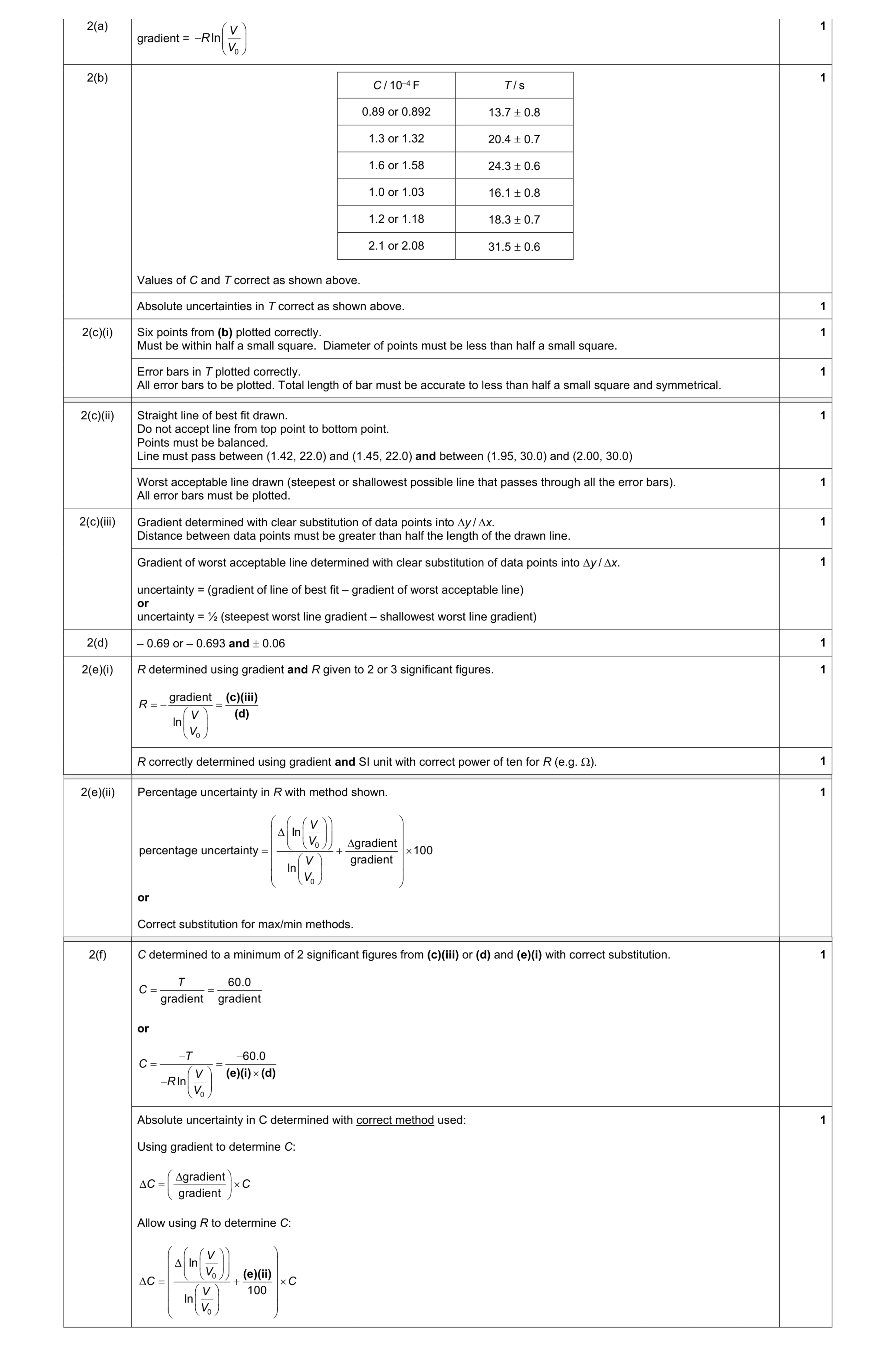 9
9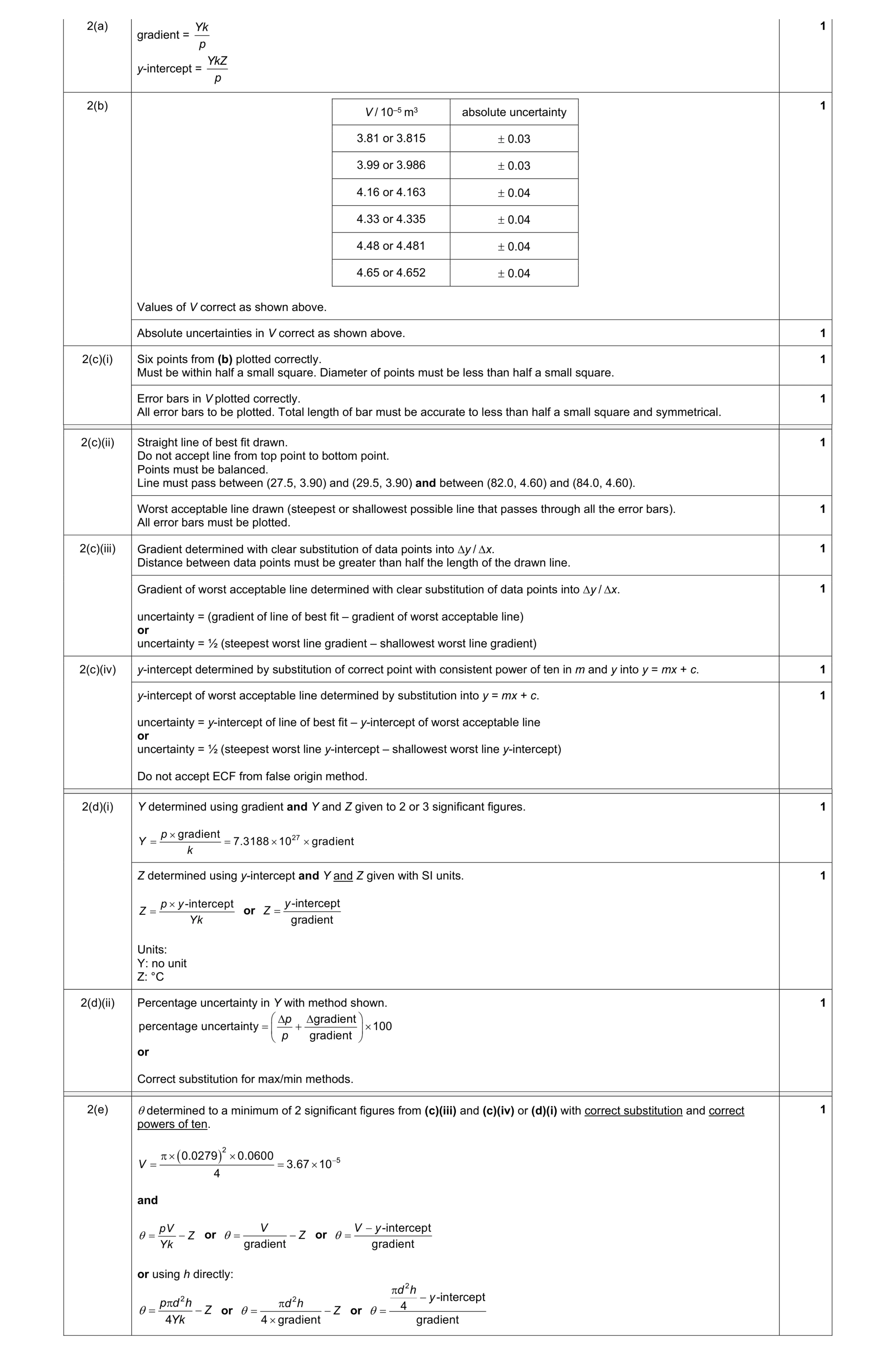 9
9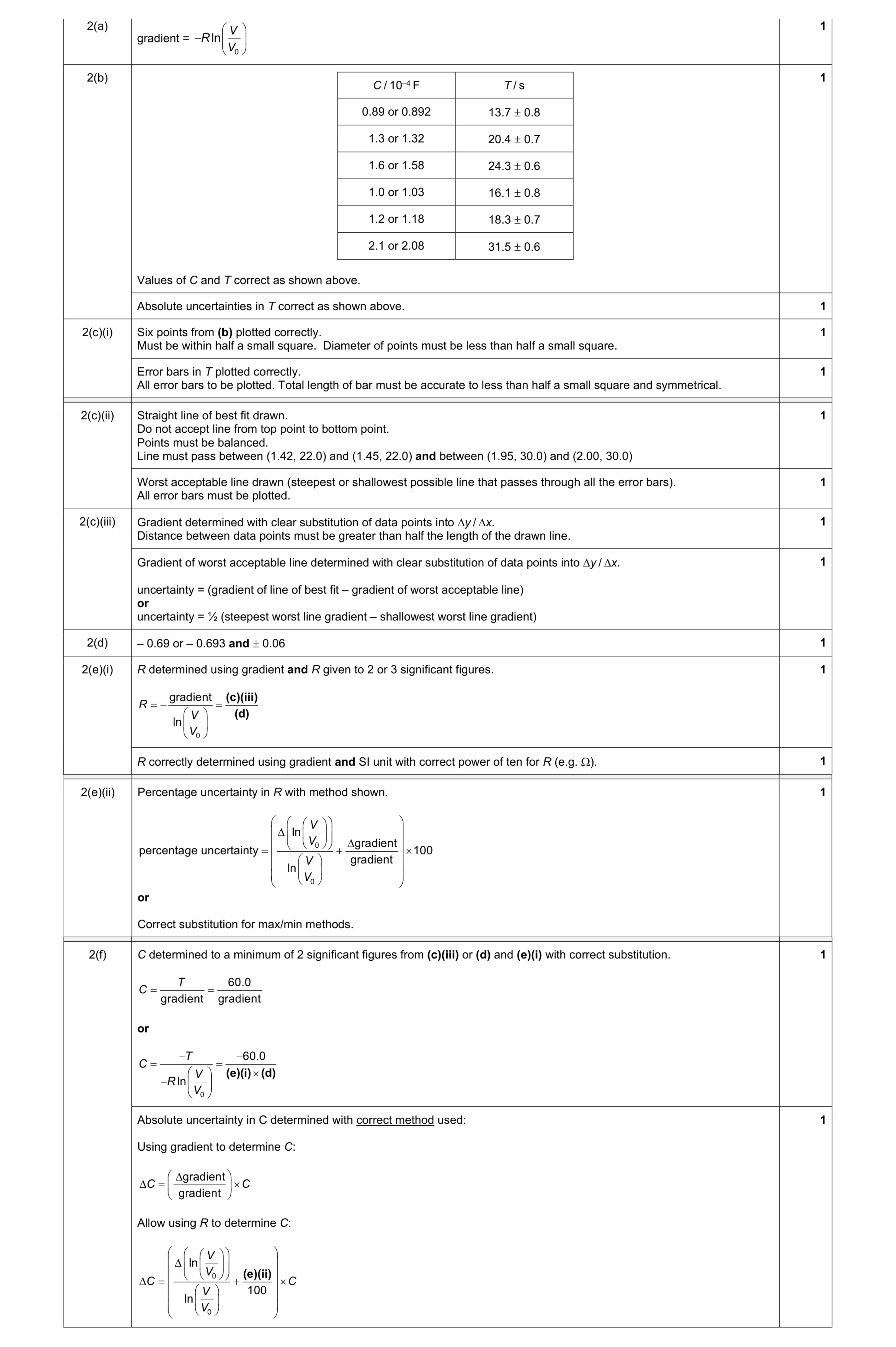 9
9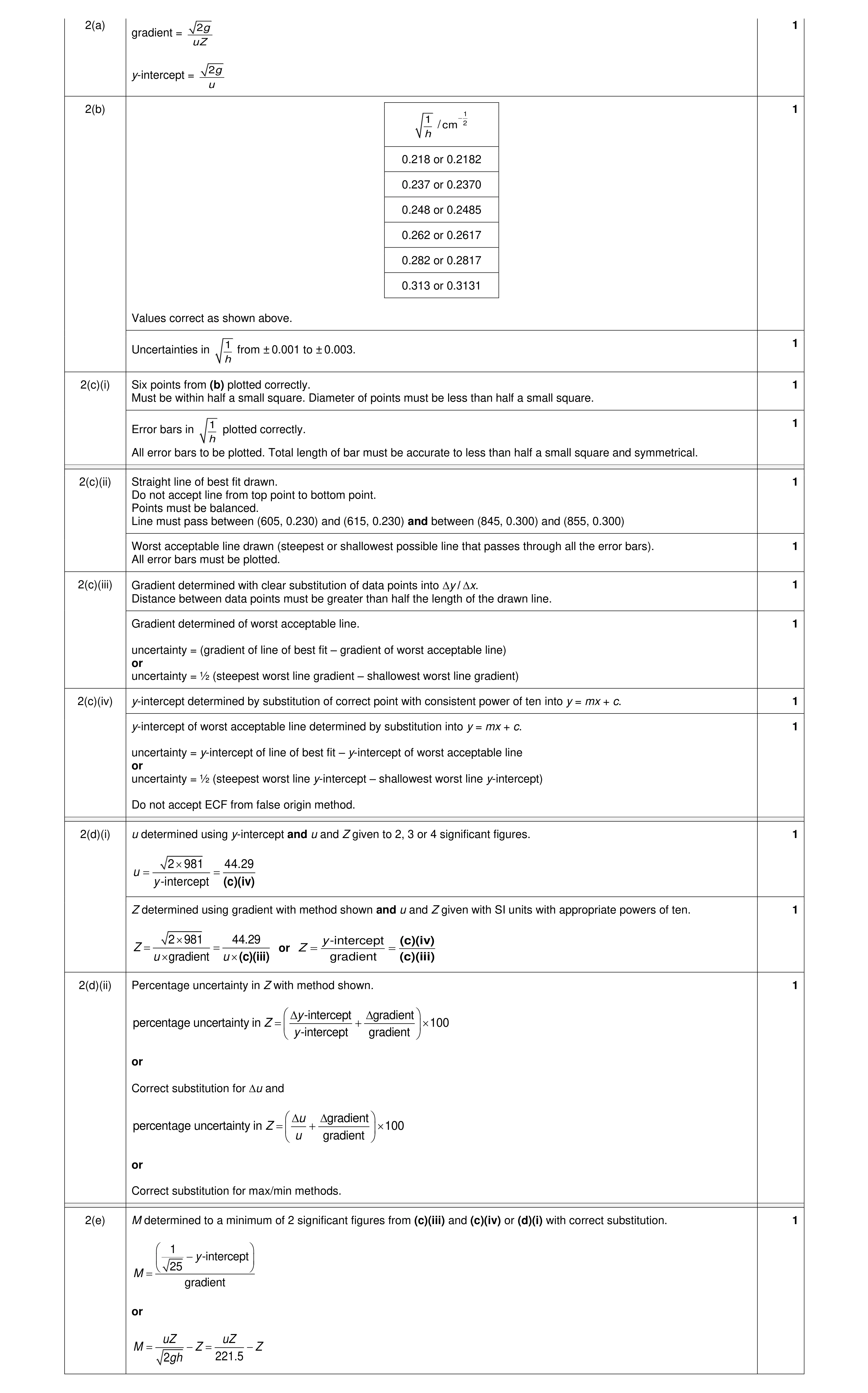 9
9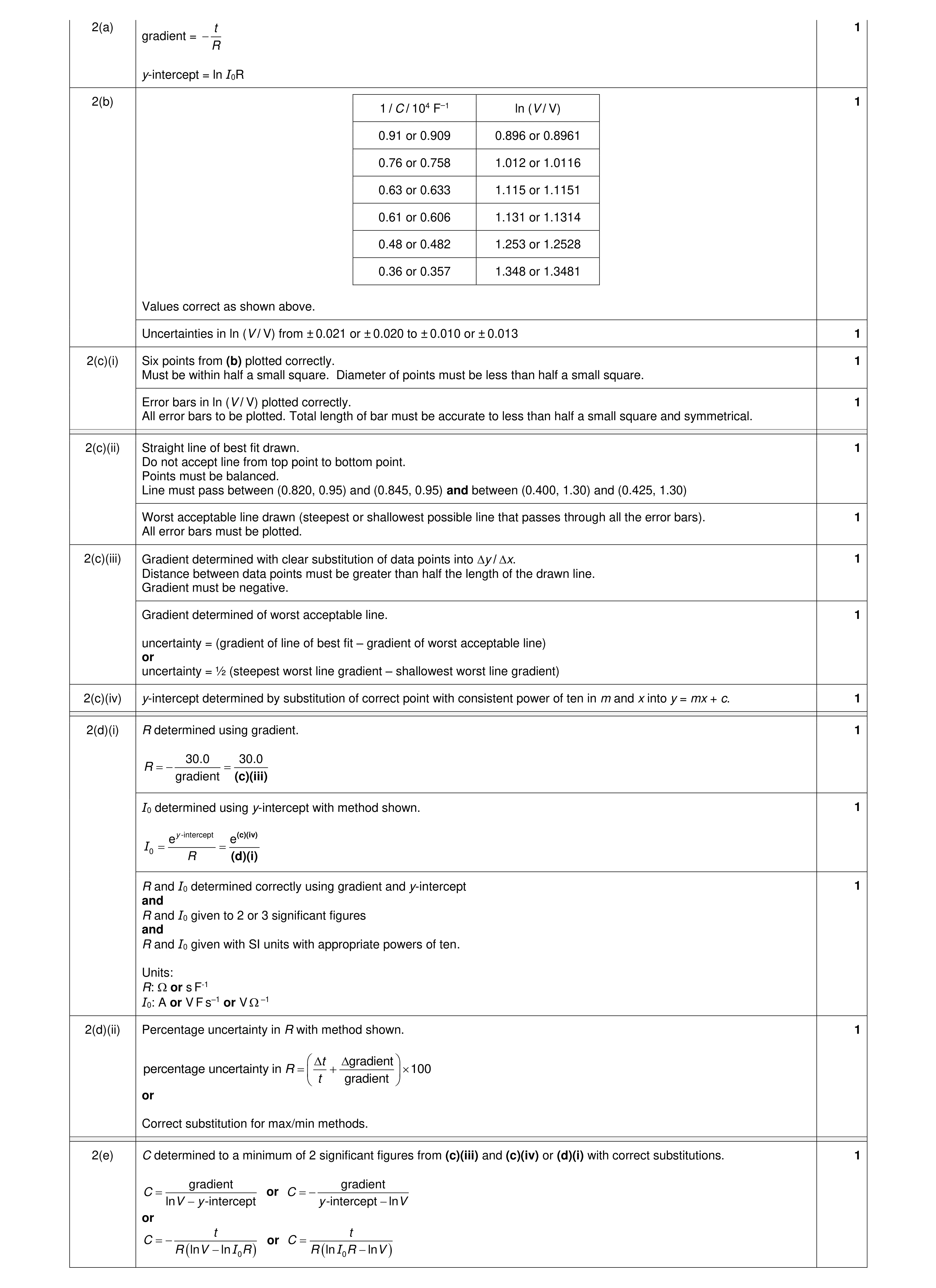 9
9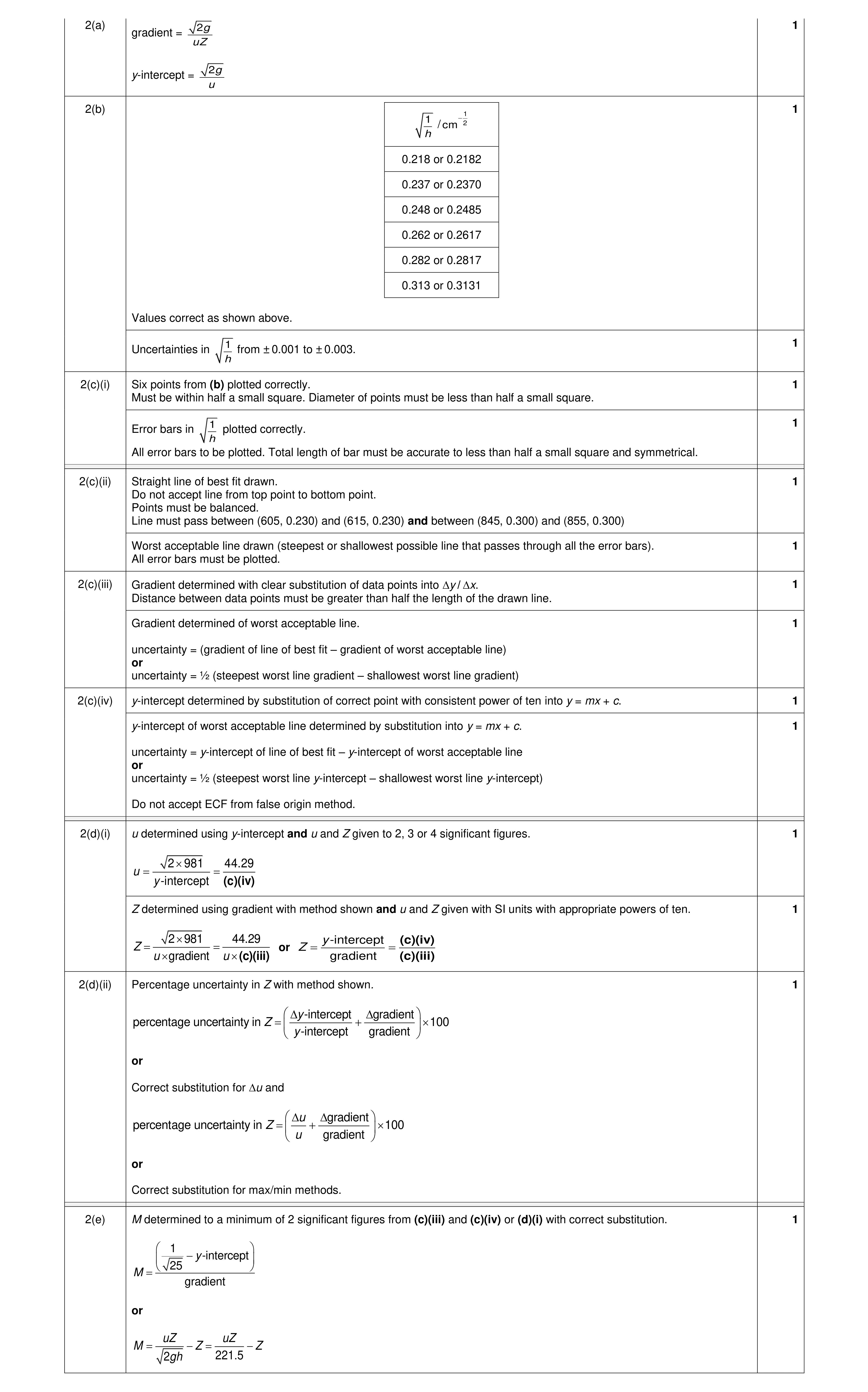 9
9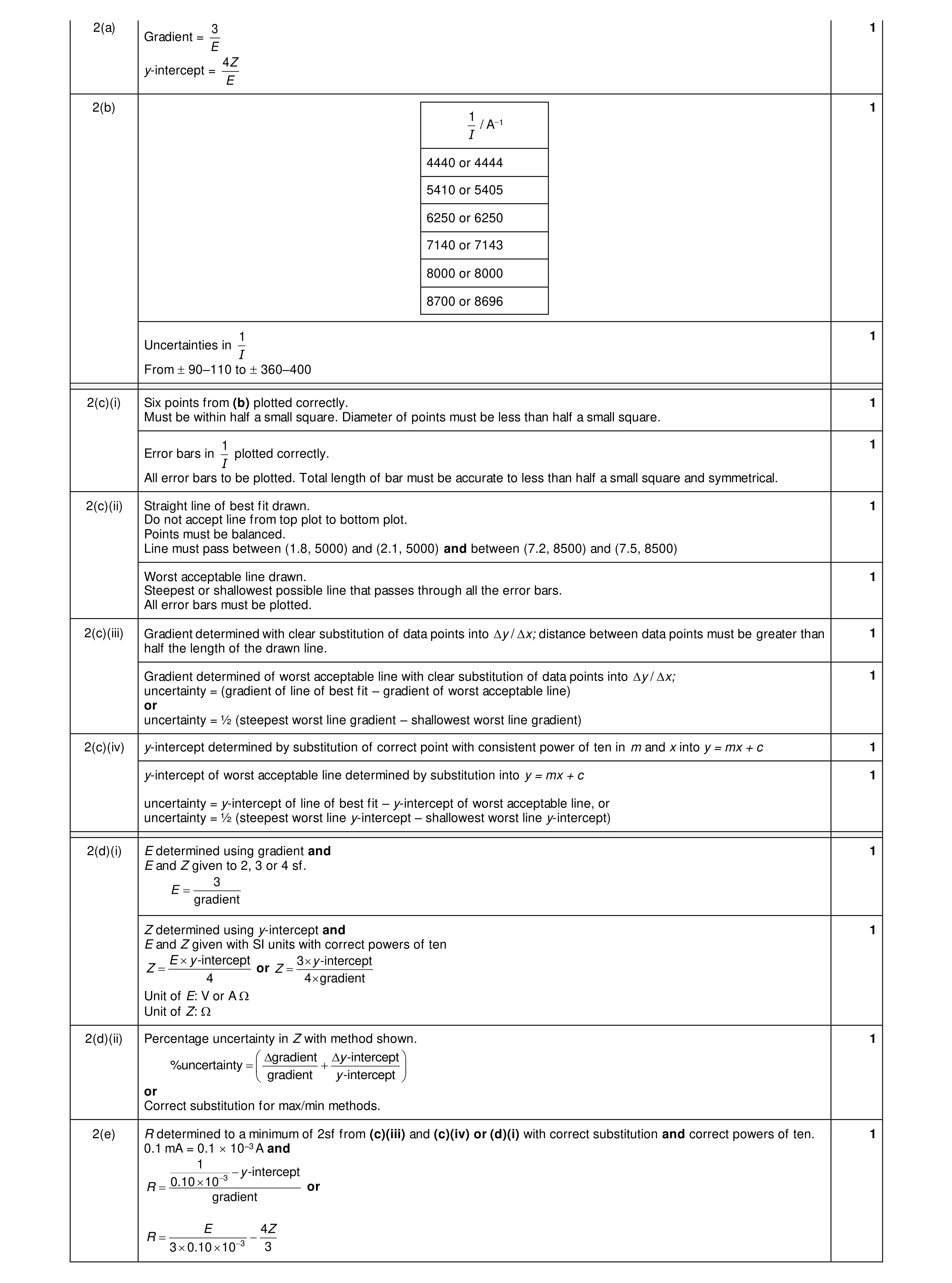 9
9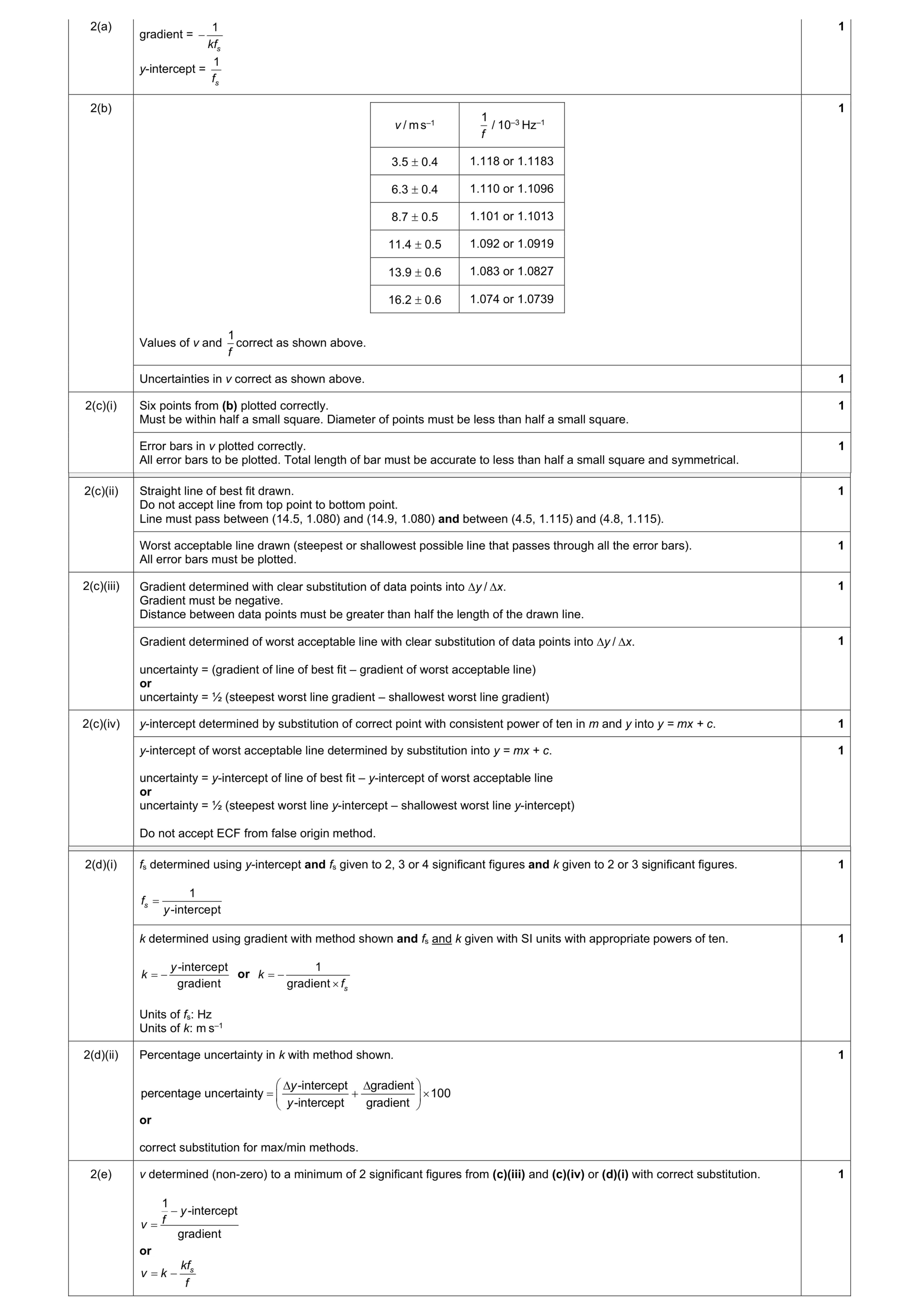 9
9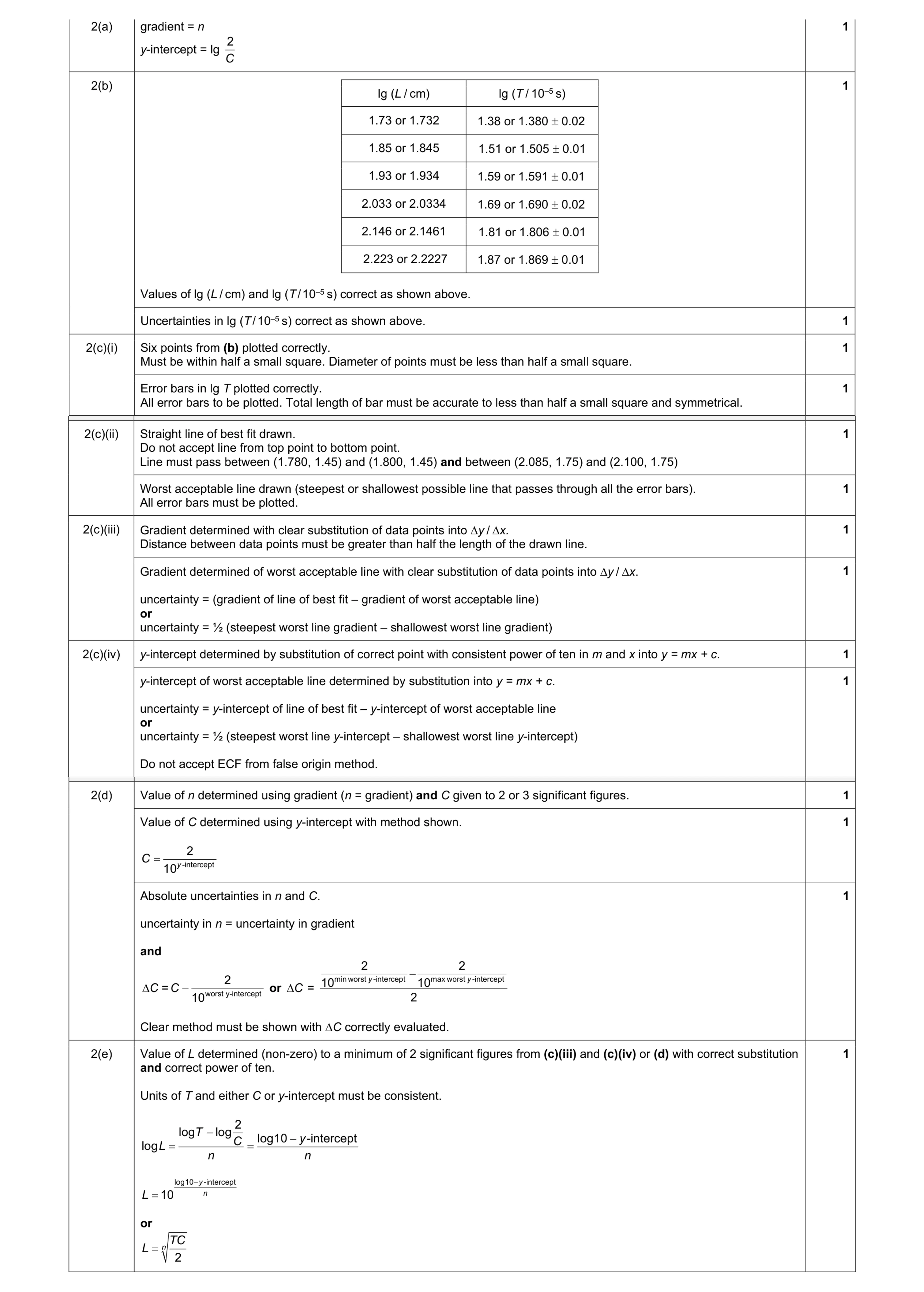 9
9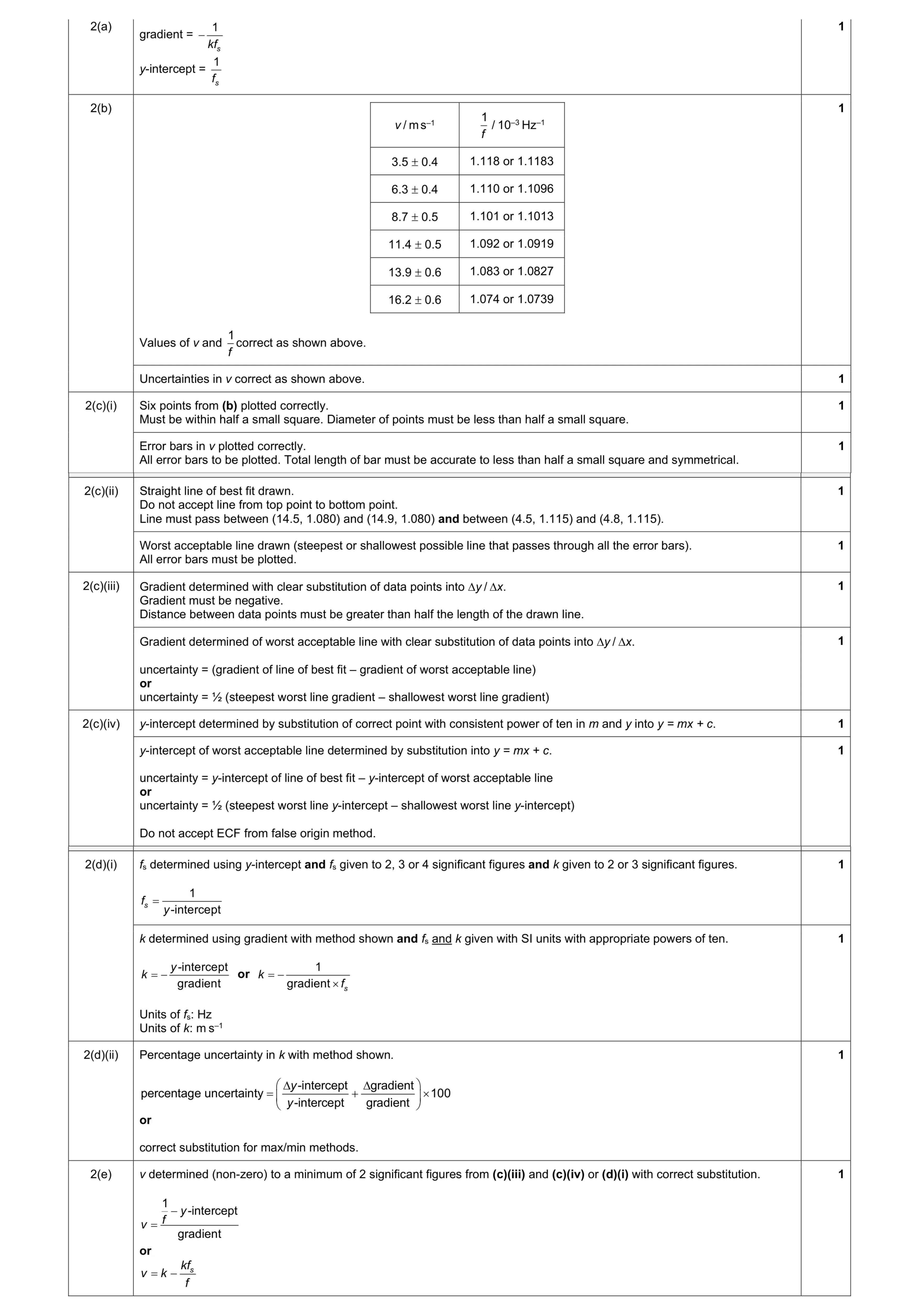 9
9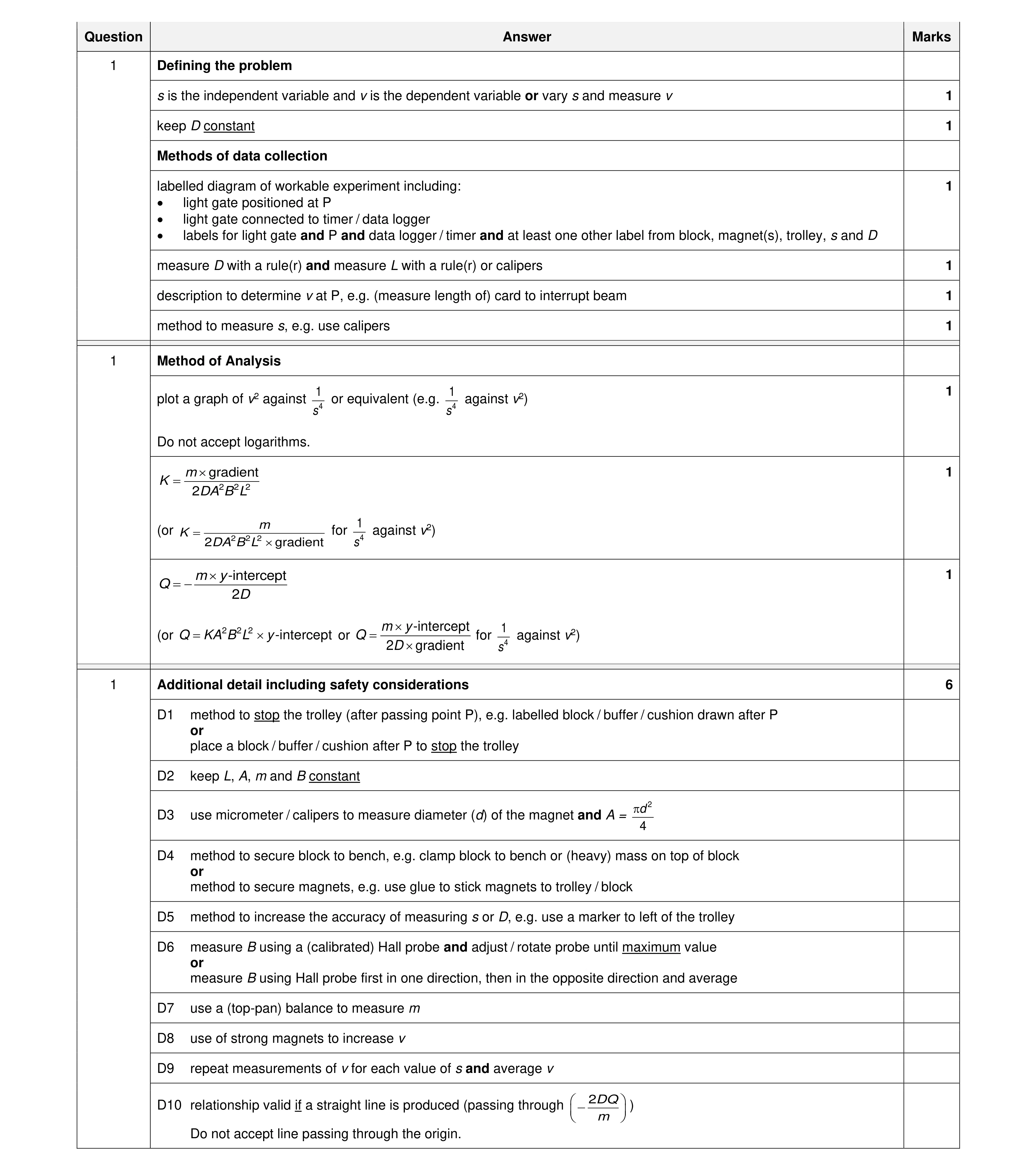 15
15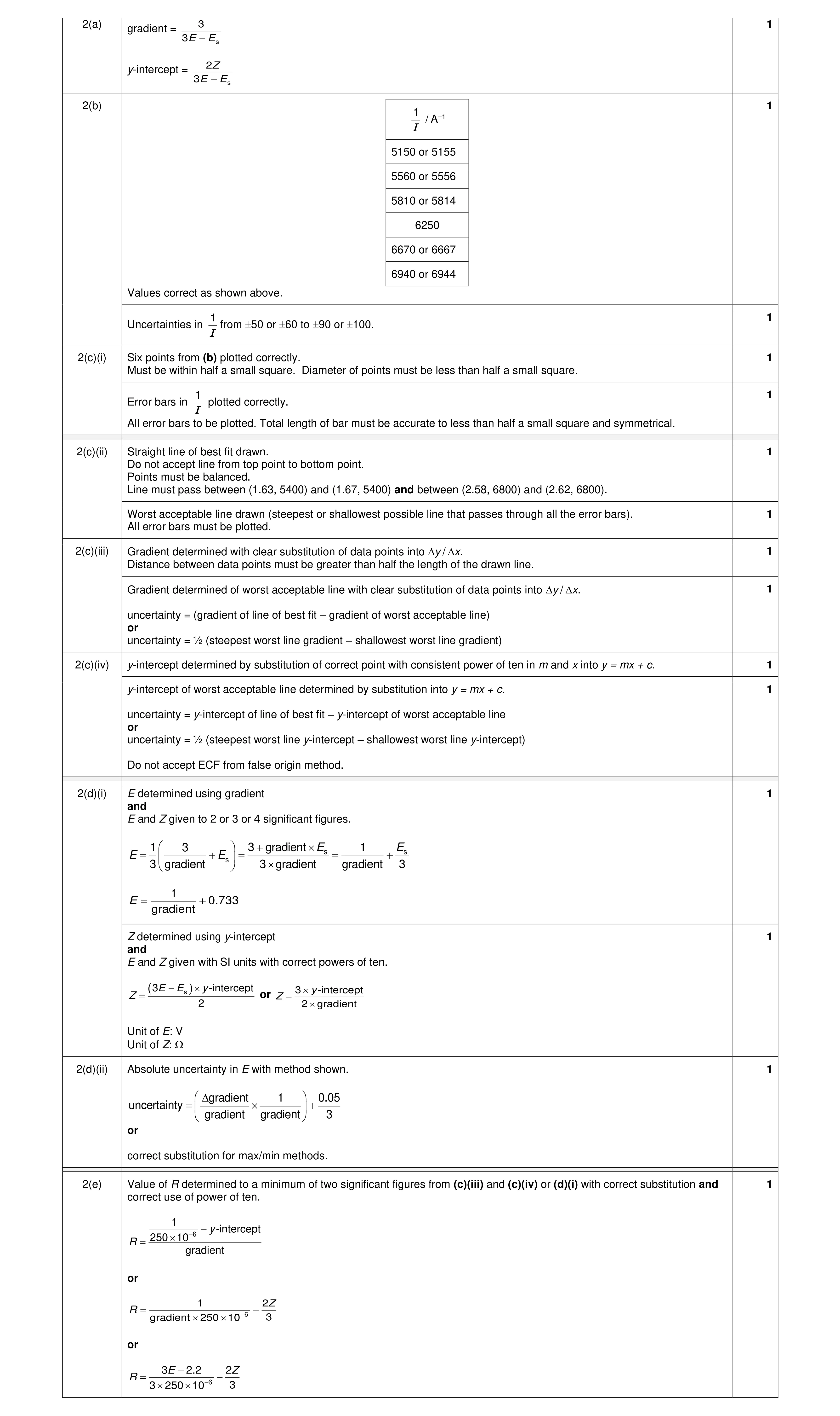 9
9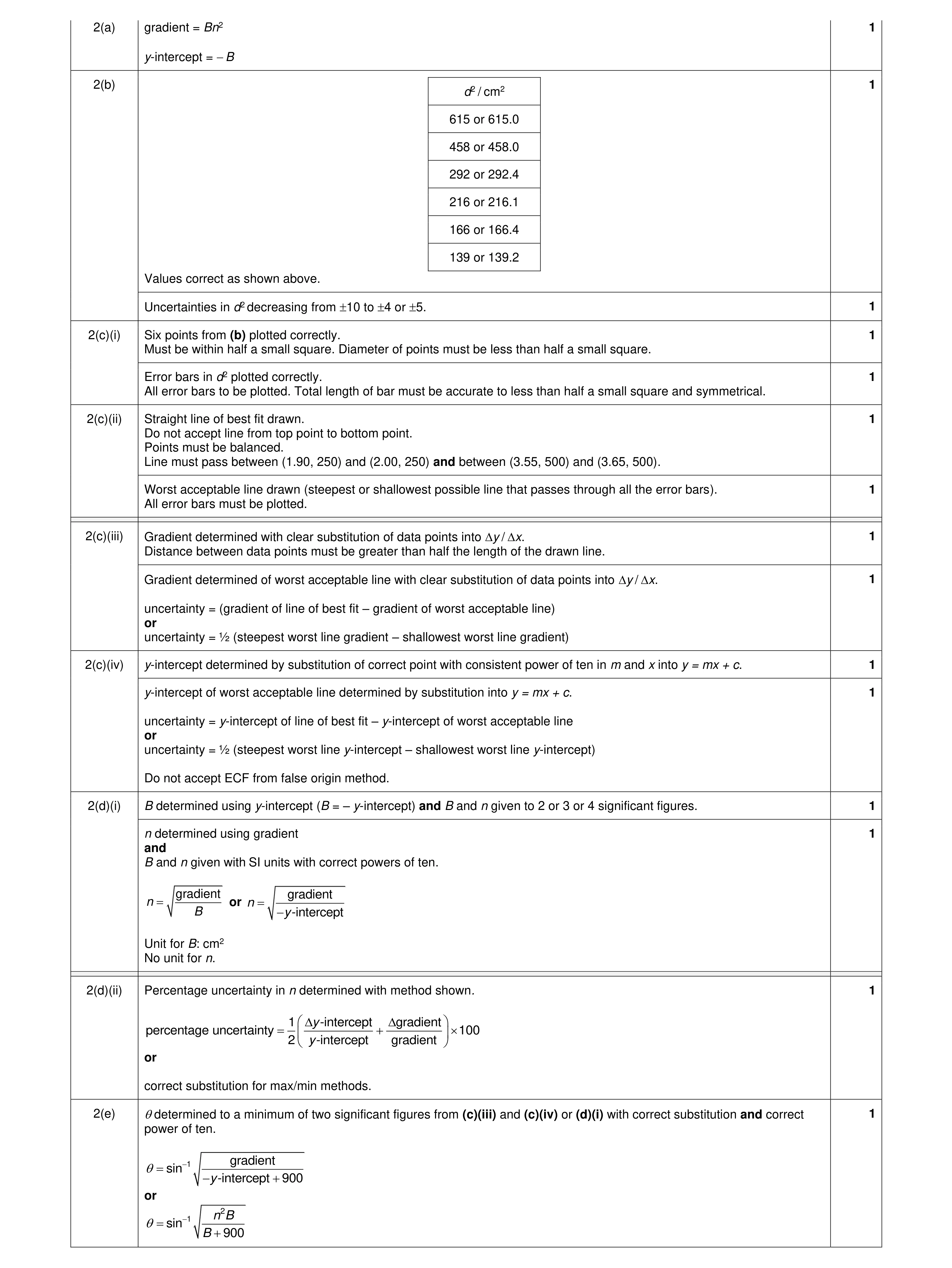 9
9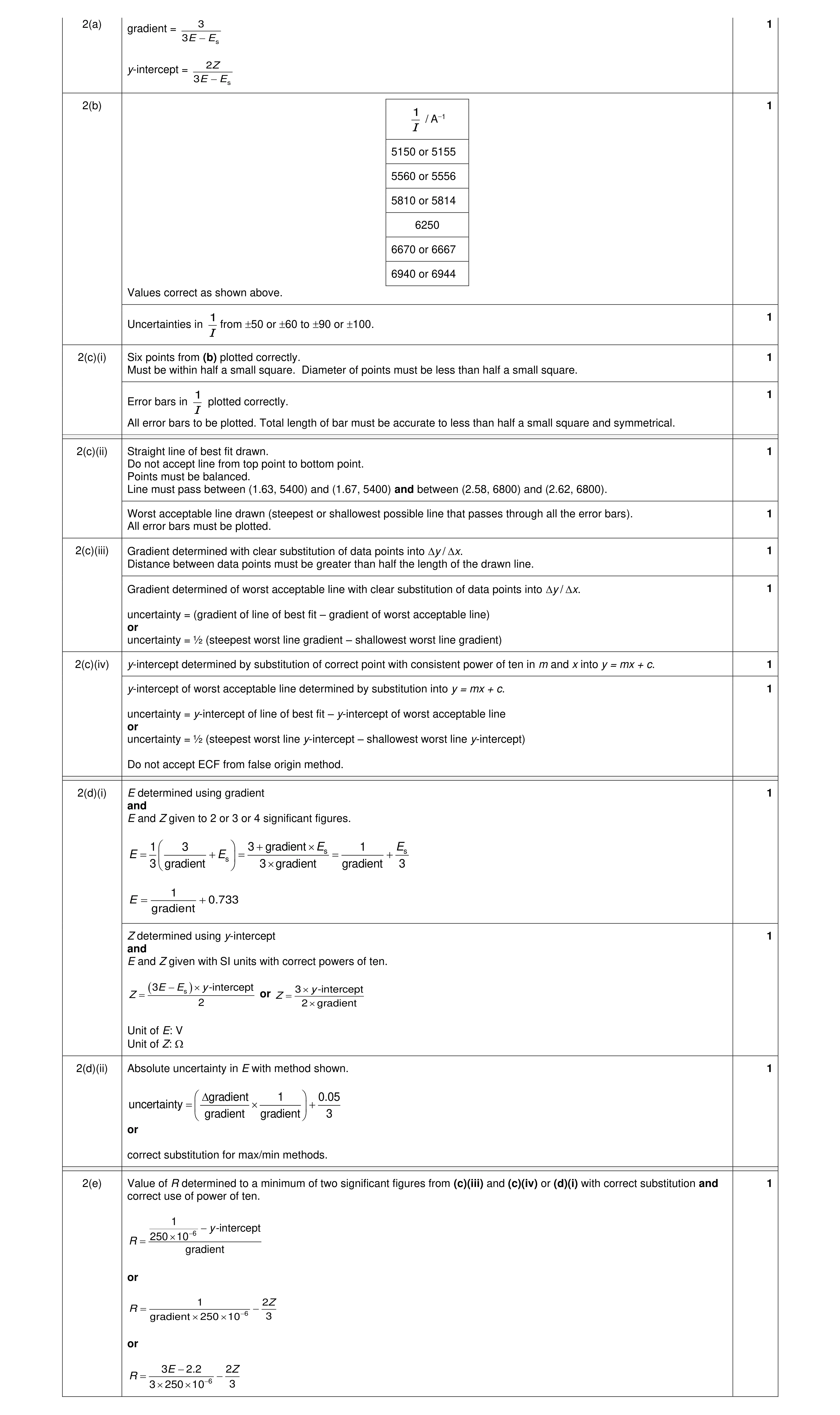 9
9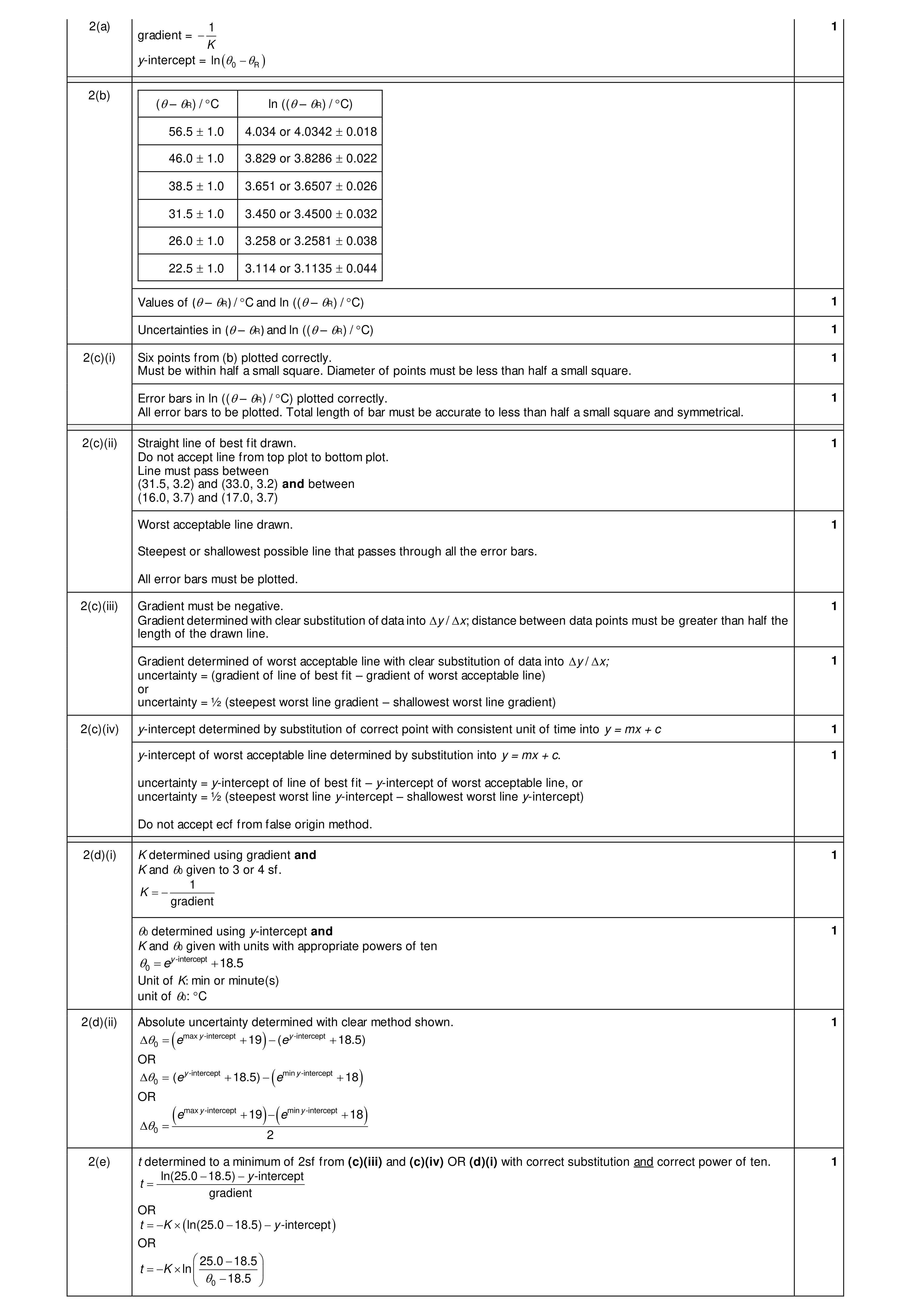 9
9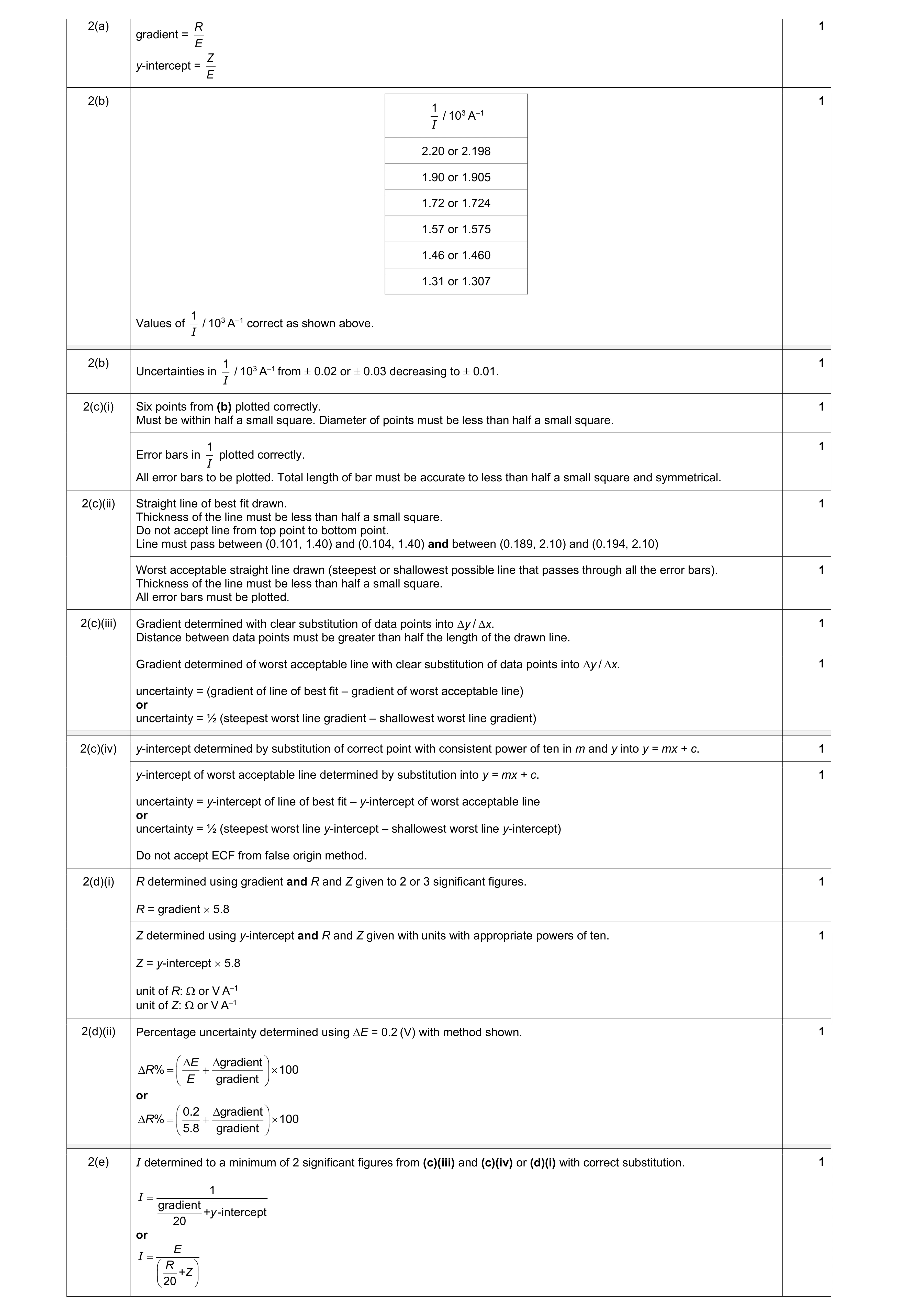 9
9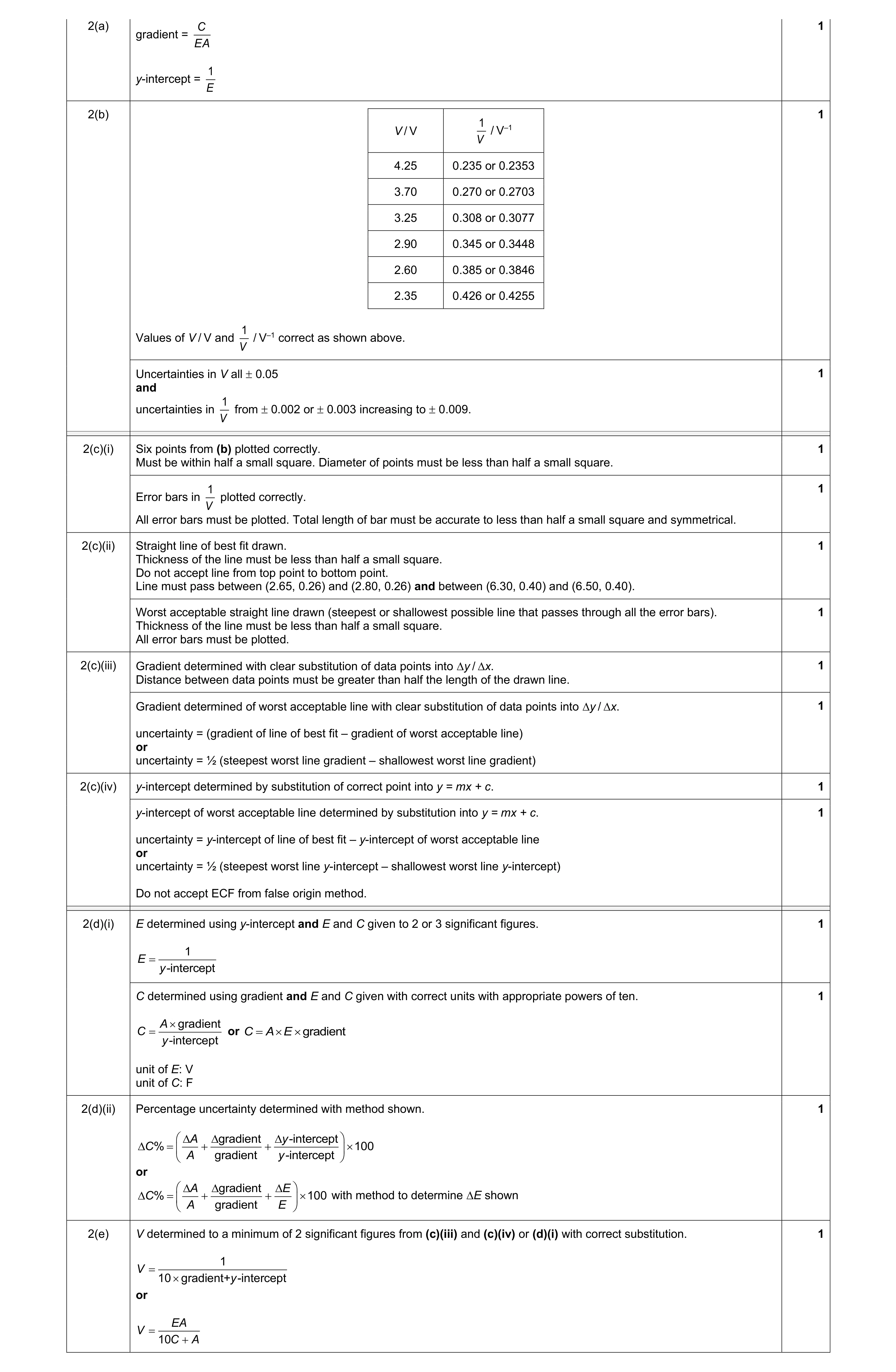 9
9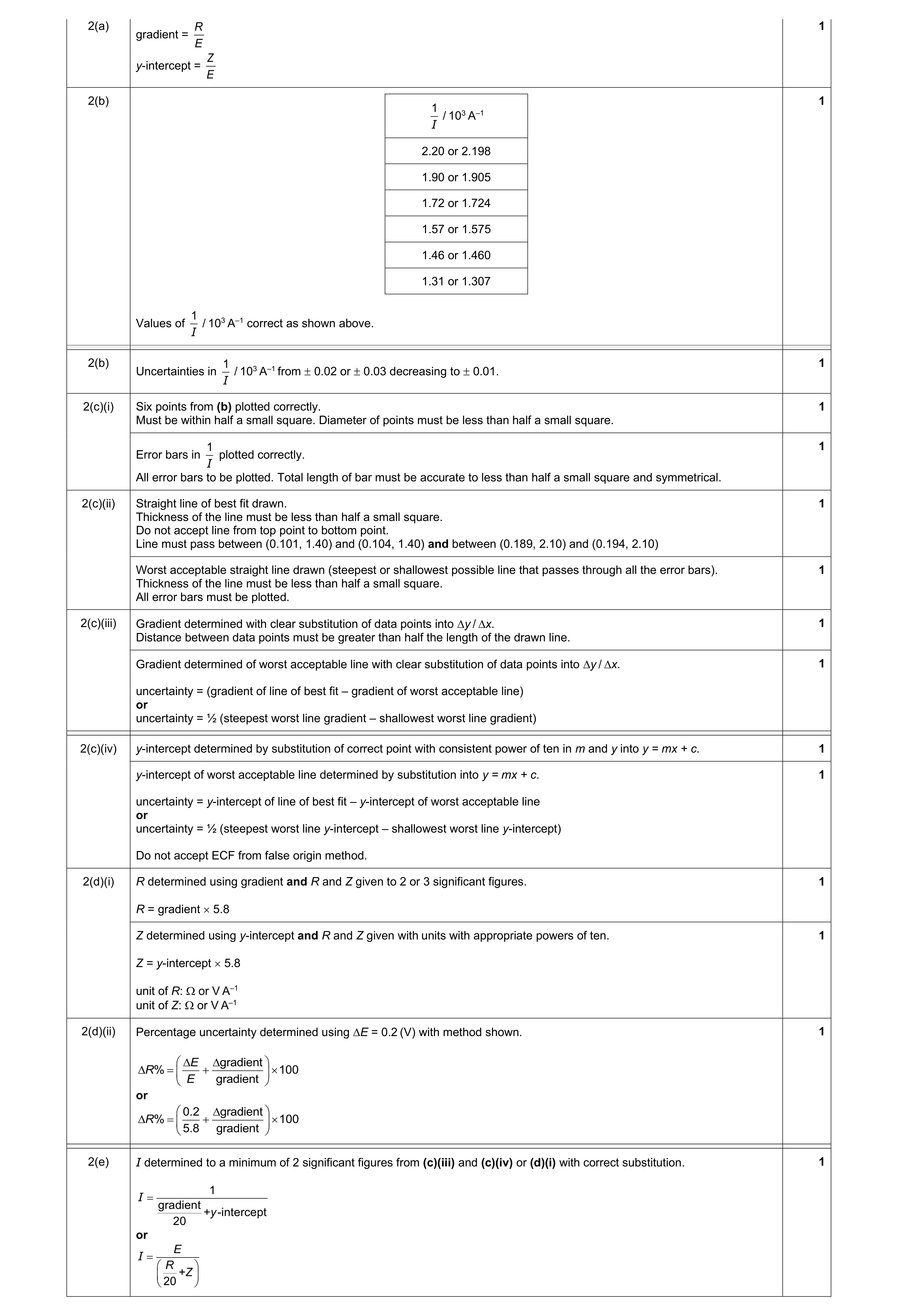 9
9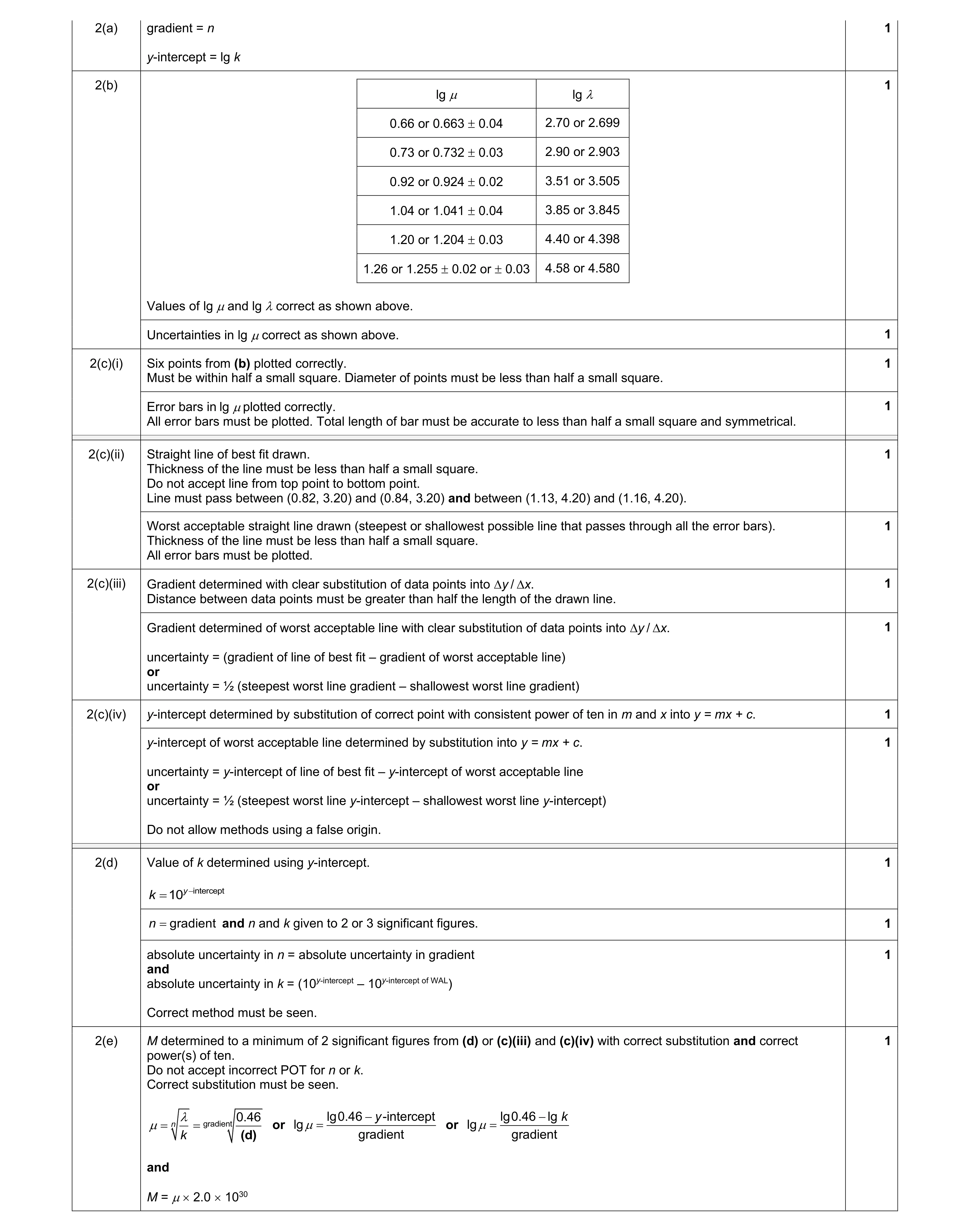 9
9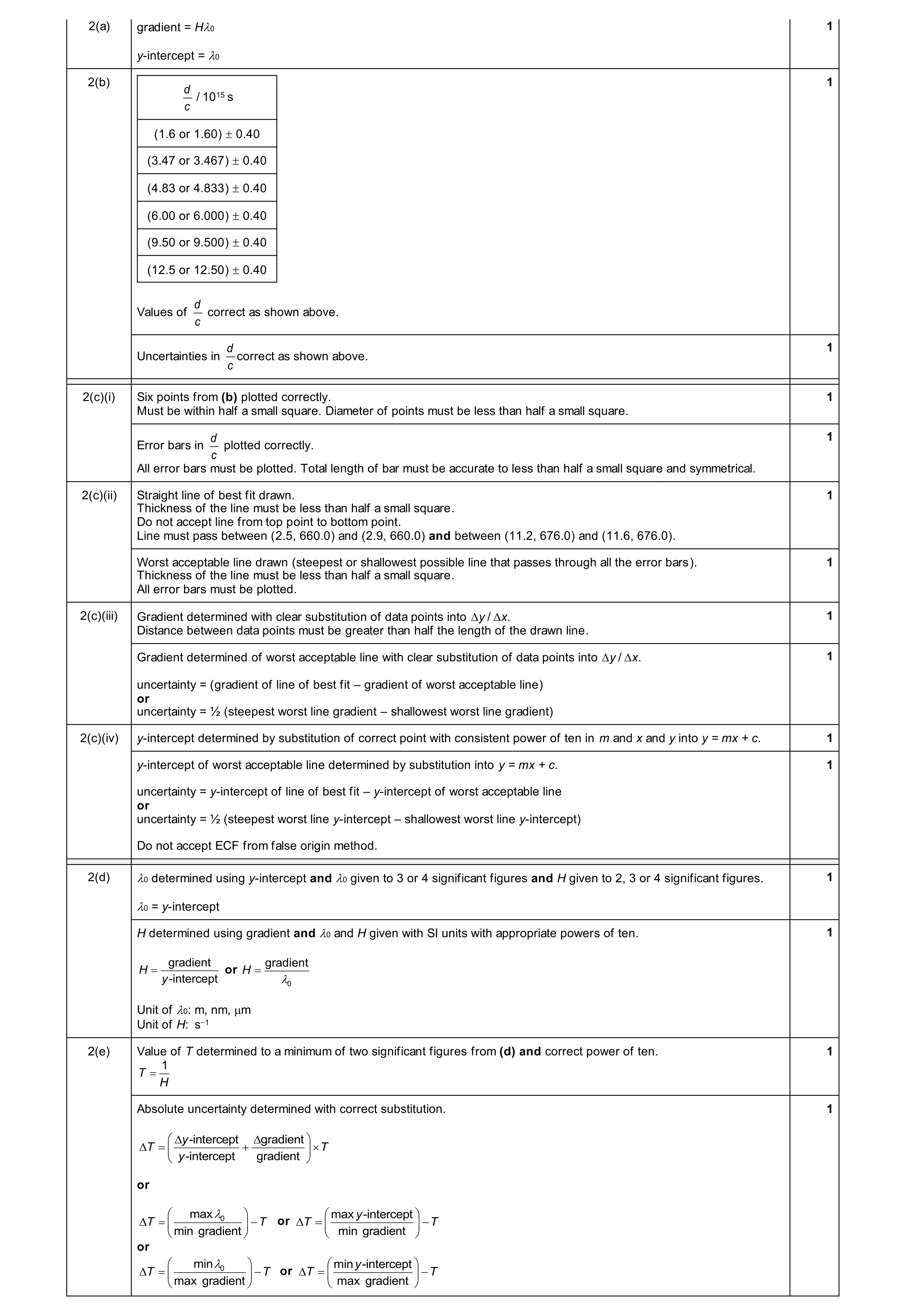 9
9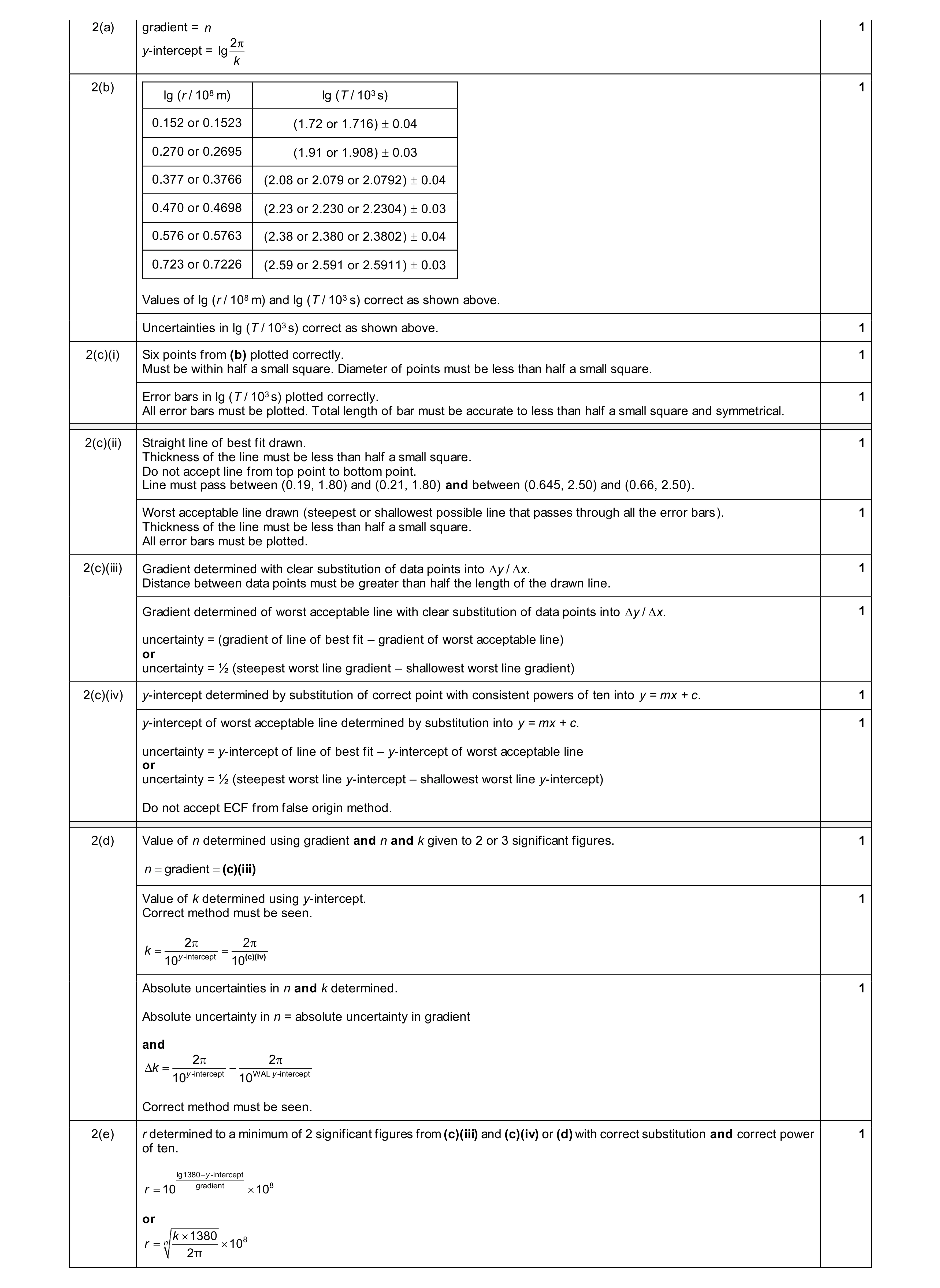 9
9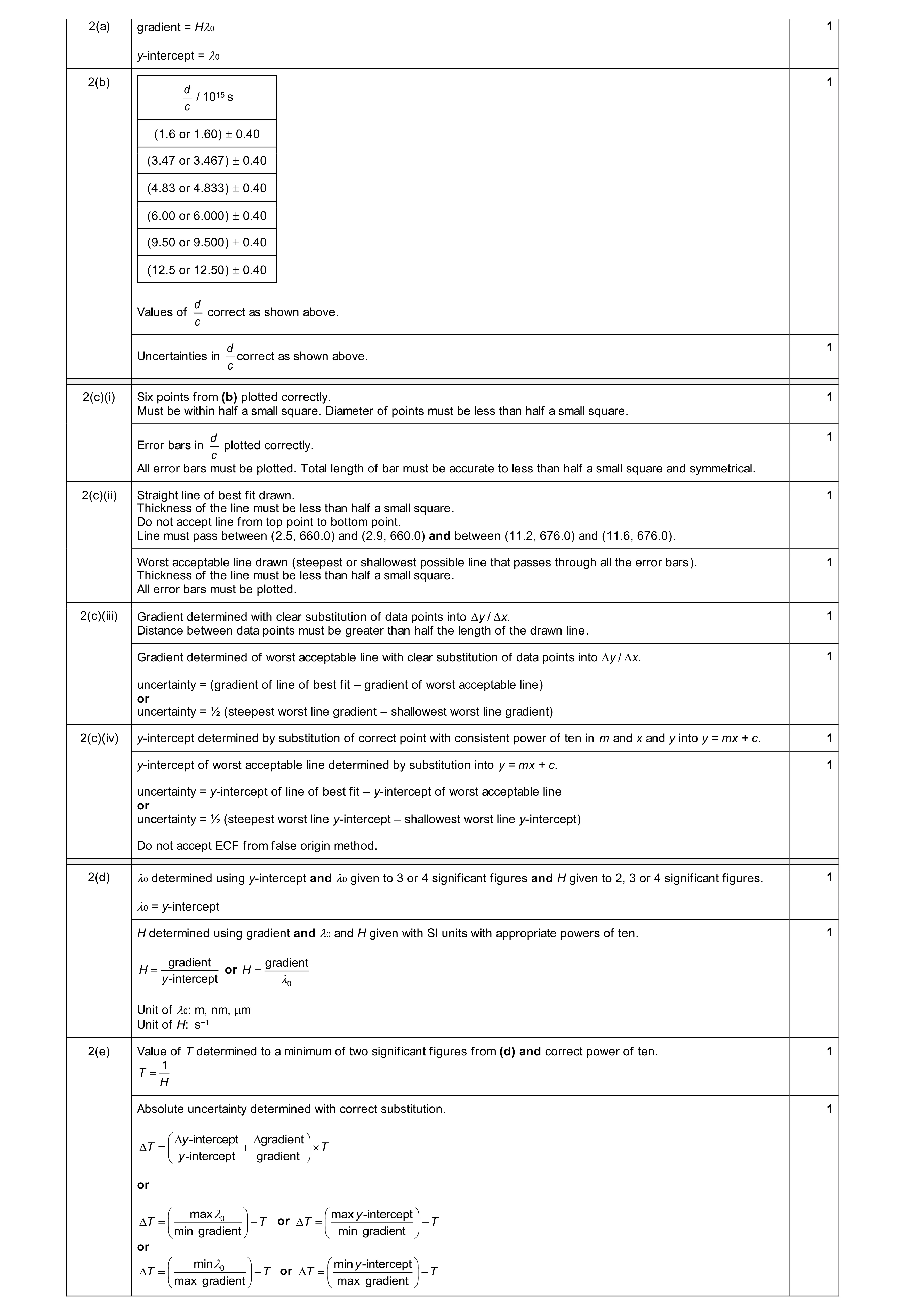 9
9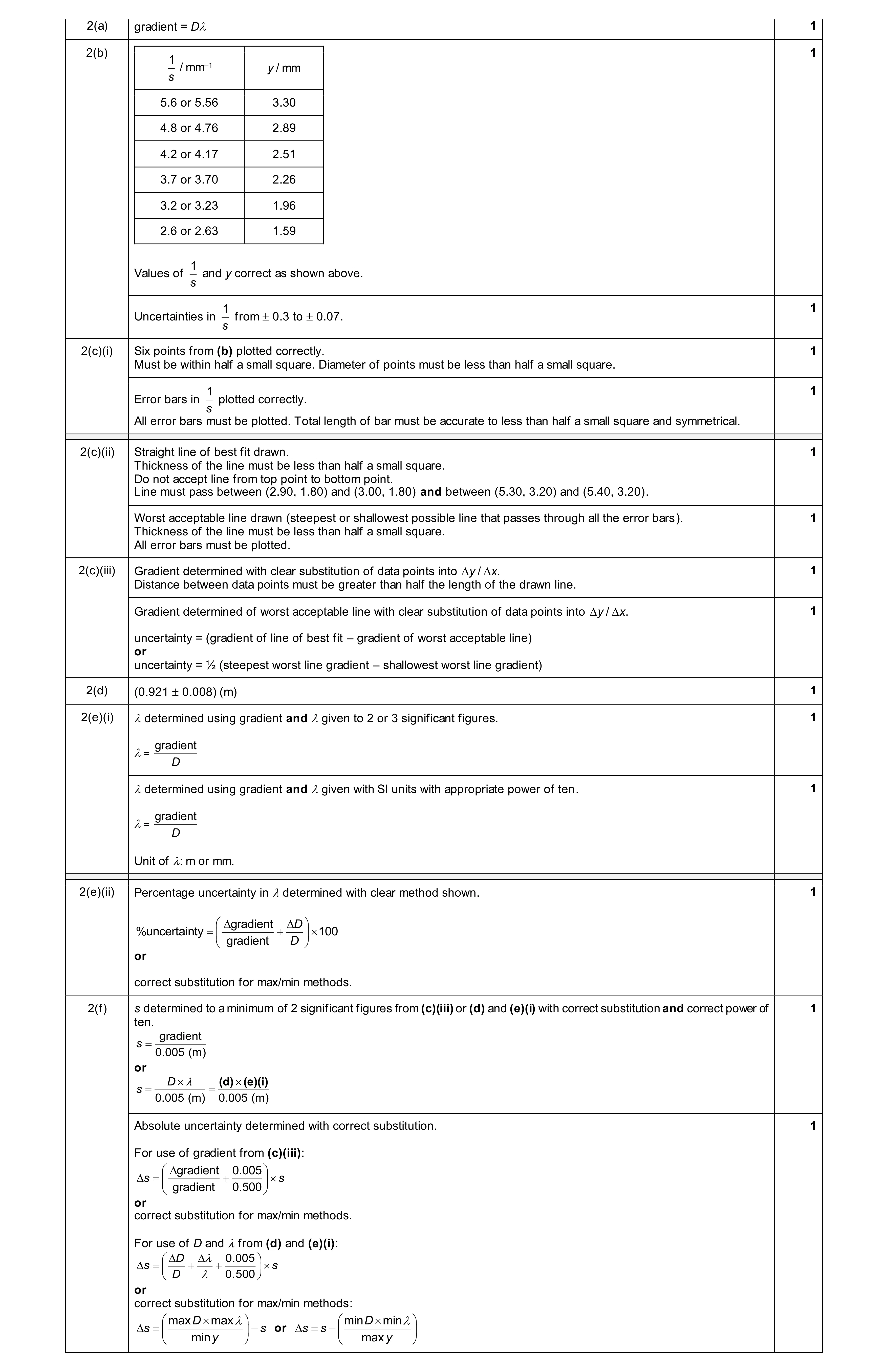 9
9