Cambridge A Level Physics 9702 — 2025 Feb/March Paper 5 · Variant 2

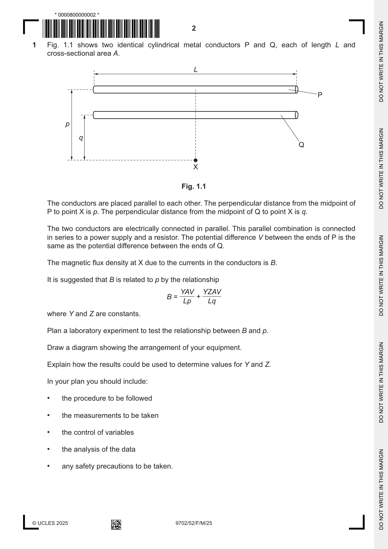
1 Fig. 1.1 shows two identical cylindrical metal conductors P and Q, each of length L and cross‑sectional area A. L P p q Q X Fig. 1.1 The conductors are placed parallel to each other. The perpendicular distance from the midpoint of P to point X is p. The perpendicular distance from the midpoint of Q to point X is q. The two conductors are electrically connected in parallel. This parallel combination is connected in series to a power supply and a resistor. The potential difference V between the ends of P is the same as the potential difference between the ends of Q. The magnetic flux density at X due to the currents in the conductors is B. It is suggested that B is related to p by the relationship YAV YZAV B = + Lp Lq where Y and Z are constants. Plan a laboratory experiment to test the relationship between B and p. Draw a diagram showing the arrangement of your equipment. Explain how the results could be used to determine values for Y and Z. In your plan you should include: • the procedure to be followed • the measurements to be taken • the control of variables • the analysis of the data • any safety precautions to be taken. Diagram .......................................................................................................................................................... .......................................................................................................................................................... .......................................................................................................................................................... .......................................................................................................................................................... .......................................................................................................................................................... .......................................................................................................................................................... .......................................................................................................................................................... .......................................................................................................................................................... .......................................................................................................................................................... .......................................................................................................................................................... .......................................................................................................................................................... .......................................................................................................................................................... .......................................................................................................................................................... .......................................................................................................................................................... .......................................................................................................................................................... .......................................................................................................................................................... .......................................................................................................................................................... .......................................................................................................................................................... .......................................................................................................................................................... .......................................................................................................................................................... .......................................................................................................................................................... .......................................................................................................................................................... .......................................................................................................................................................... .......................................................................................................................................................... .......................................................................................................................................................... .......................................................................................................................................................... .......................................................................................................................................................... .......................................................................................................................................................... .......................................................................................................................................................... .......................................................................................................................................................... .......................................................................................................................................................... .......................................................................................................................................................... .......................................................................................................................................................... .......................................................................................................................................................... .......................................................................................................................................................... .......................................................................................................................................................... .......................................................................................................................................................... .......................................................................................................................................................... .......................................................................................................................................................... .......................................................................................................................................................... .......................................................................................................................................................... .................................................................................................................................................. [15]

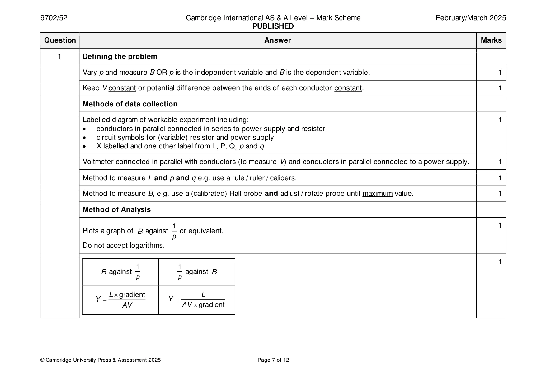
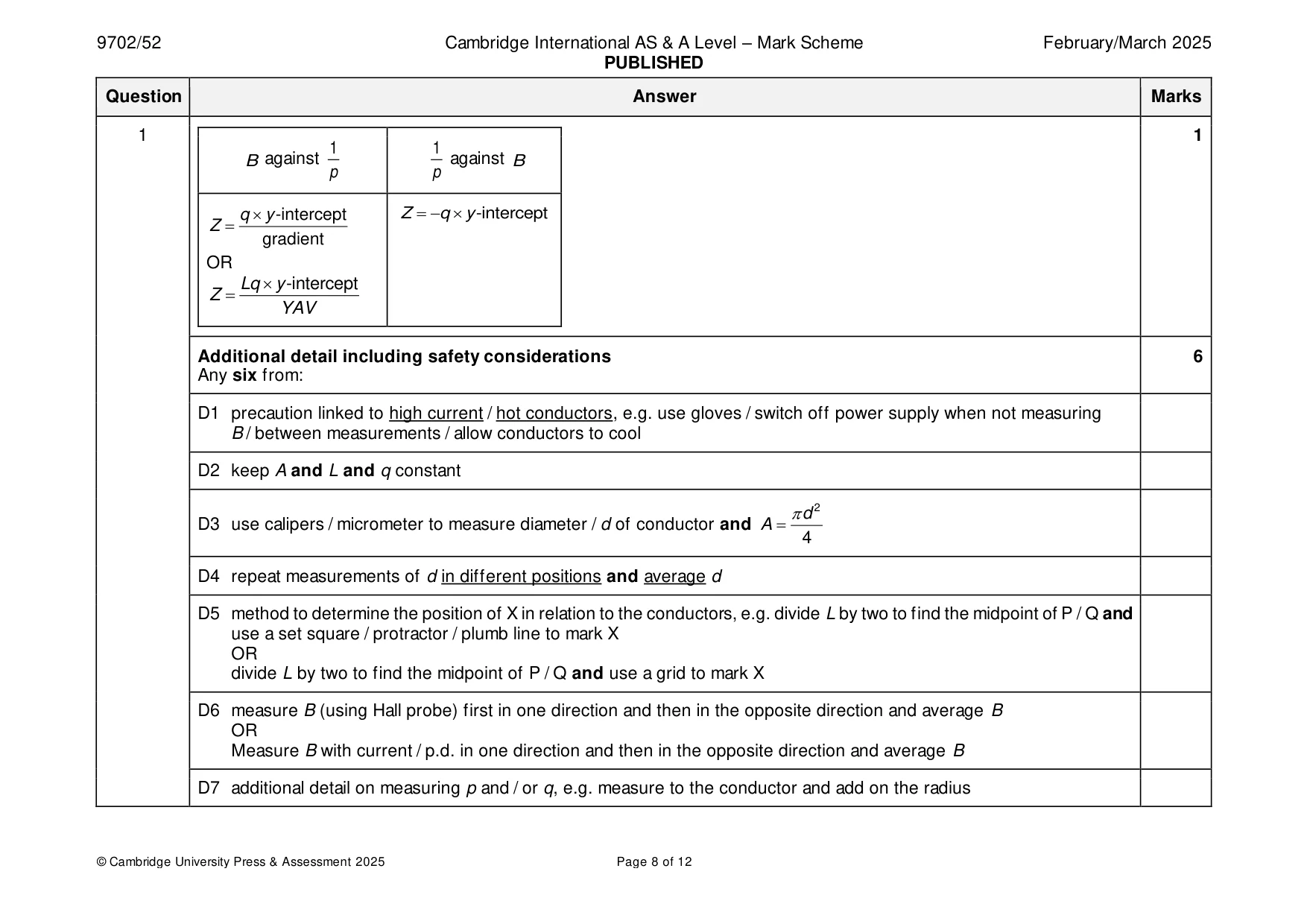
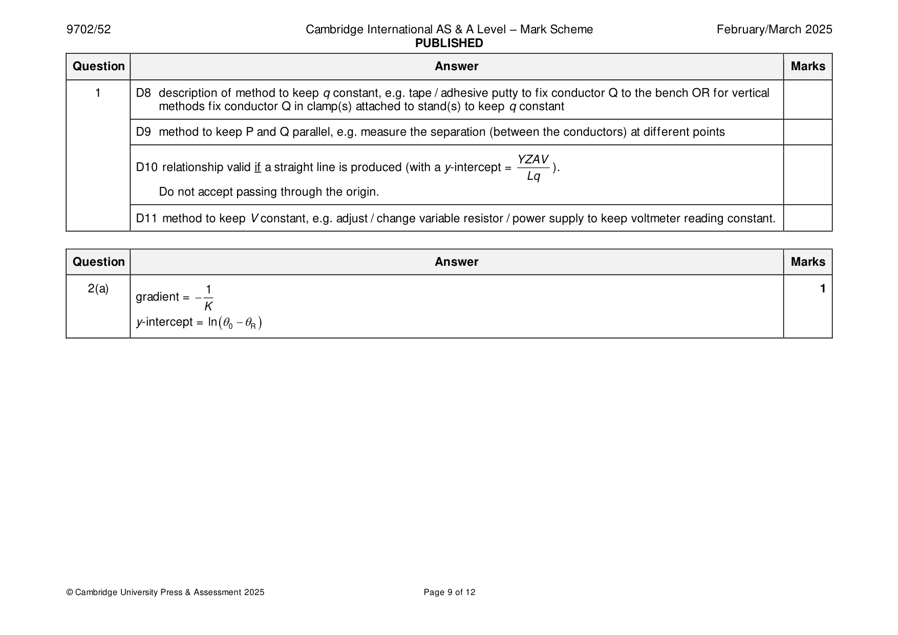
Mark scheme: Question Answer Marks 1 Defining the problem Vary p and measure B OR p is the independent variable and B is the dependent variable. 1 Keep V constant or potential difference between the ends of each conductor constant. 1 Methods of data collection Labelled diagram of workable experiment including: 1 • conductors in parallel connected in series to power supply and resistor • circuit symbols for (variable) resistor and power supply • X labelled and one other label from L, P, Q, p and q. Voltmeter connected in parallel with conductors (to measure V) and conductors in parallel connected to a power supply. 1 Method to measure L and p and q e.g. use a rule / ruler / calipers. 1 Method to measure B, e.g. use a (calibrated) Hall probe and adjust / rotate probe until maximum value. 1 Method of Analysis 1 1 Plots a graph of B against or equivalent. p Do not accept logarithms. 1 1 1 B against against B p p L  gradient L Y = Y = AV AV  gradient 1 1 1 1 B against against B p p q  y -intercept Z = −q y -intercept Z = gradient OR Lq  y -intercept Z = YAV Additional detail including safety considerations 6 Any six from: D1 precaution linked to high current / hot conductors, e.g. use gloves / switch off power supply when not measuring B / between measurements / allow conductors to cool D2 keep A and L and q constant d 2 D3 use calipers / micrometer to measure diameter / d of conductor and A = 4 D4 repeat measurements of d in different positions and average d D5 method to determine the position of X in relation to the conductors, e.g. divide L by two to find the midpoint of P / Q and use a set square / protractor / plumb line to mark X OR divide L by two to find the midpoint of P / Q and use a grid to mark X D6 measure B (using Hall probe) first in one direction and then in the opposite direction and average B OR Measure B with current / p.d. in one direction and then in the opposite direction and average B D7 additional detail on measuring p and / or q, e.g. measure to the conductor and add on the radius 1 D8 description of method to keep q constant, e.g. tape / adhesive putty to fix conductor Q to the bench OR for vertical methods fix conductor Q in clamp(s) attached to stand(s) to keep q constant D9 method to keep P and Q parallel, e.g. measure the separation (between the conductors) at different points YZAV D10 relationship valid if a straight line is produced (with a y-intercept = ). Lq Do not accept passing through the origin. D11 method to keep V constant, e.g. adjust / change variable resistor / power supply to keep voltmeter reading constant.

More questions on Magnetic fields due to currents

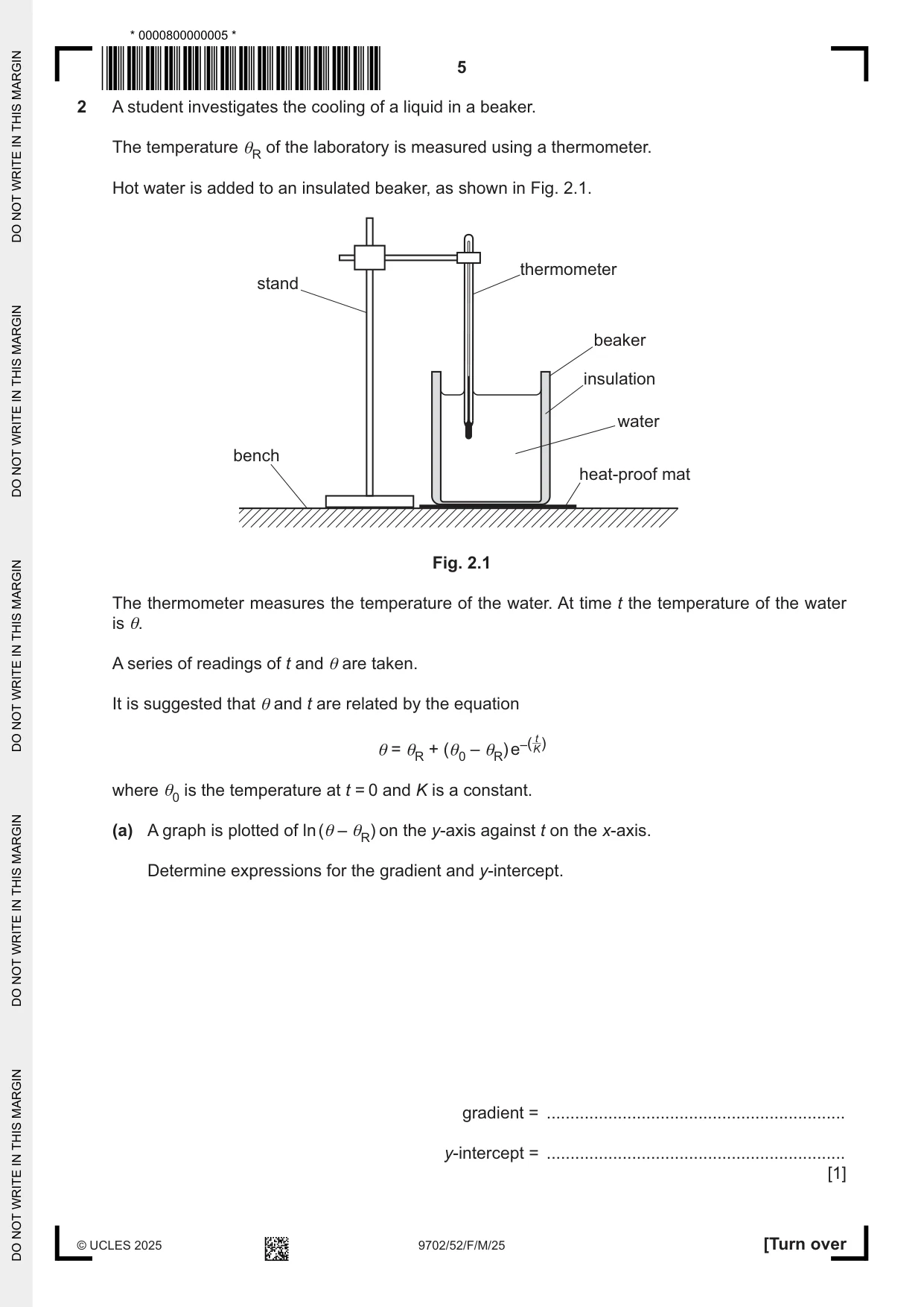
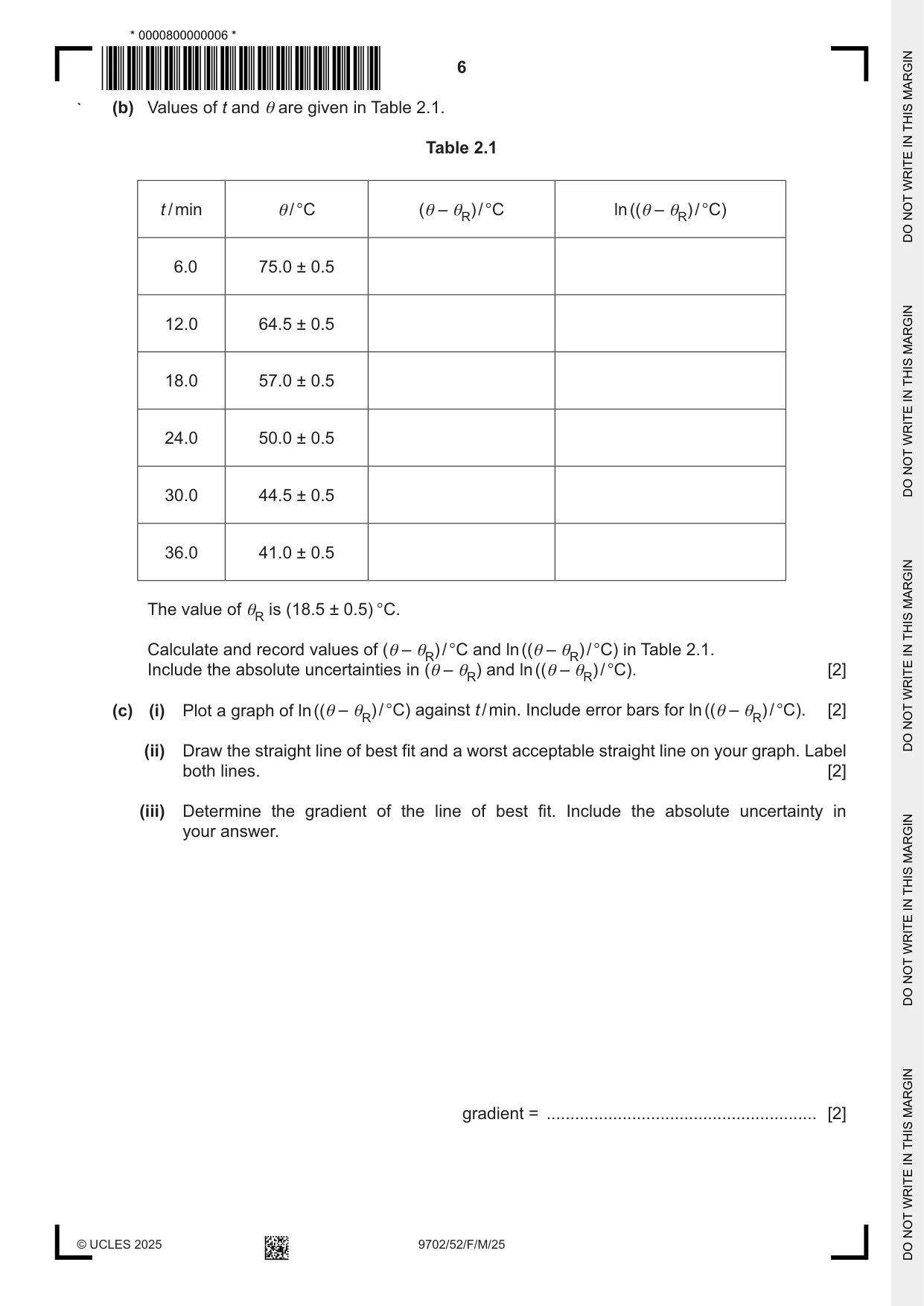
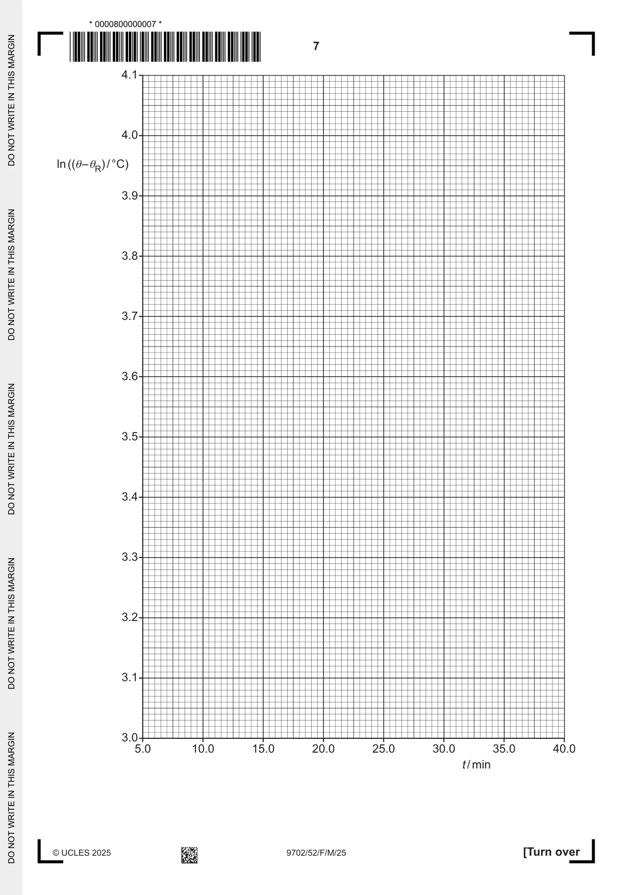
2 A student investigates the cooling of a liquid in a beaker. The temperature θR of the laboratory is measured using a thermometer. Hot water is added to an insulated beaker, as shown in Fig. 2.1. thermometer stand beaker insulation water bench heat-proof mat Fig. 2.1 The thermometer measures the temperature of the water. At time t the temperature of the water is θ. A series of readings of t and θ are taken. It is suggested that θ and t are related by the equation θ = + – e–( K)t θR (θ0 θR) where θ0 is the temperature at t = 0 and K is a constant. (a) A graph is plotted of ln (θ – θR) on the y‑axis against t on the x‑axis. Determine expressions for the gradient and y‑intercept. gradient = ............................................................... y‑intercept = ............................................................... [1] ` (b) Values of t and θ are given in Table 2.1. Table 2.1 t / min θ/ °C (θ – θR) / °C ln ((θ – θR) / °C) 6.0 75.0 ± 0.5 12.0 64.5 ± 0.5 18.0 57.0 ± 0.5 24.0 50.0 ± 0.5 30.0 44.5 ± 0.5 36.0 41.0 ± 0.5 The value of θR is (18.5 ± 0.5) °C. Calculate and record values of (θ – θR) / °C and ln ((θ – θR) / °C) in Table 2.1. Include the absolute uncertainties in (θ – θR) and ln ((θ – θR) / °C). [2] (c) (i) Plot a graph of ln ((θ – θR) / °C) against t / min. Include error bars for ln ((θ – θR) / °C). [2] (ii) Draw the straight line of best fit and a worst acceptable straight line on your graph. Label both lines. [2] (iii) Determine the gradient of the line of best fit. Include the absolute uncertainty in your answer. gradient = ......................................................... [2]

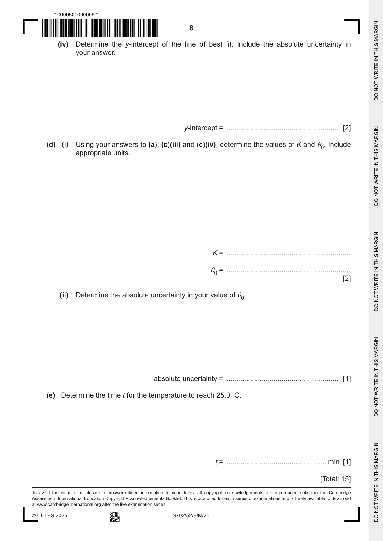
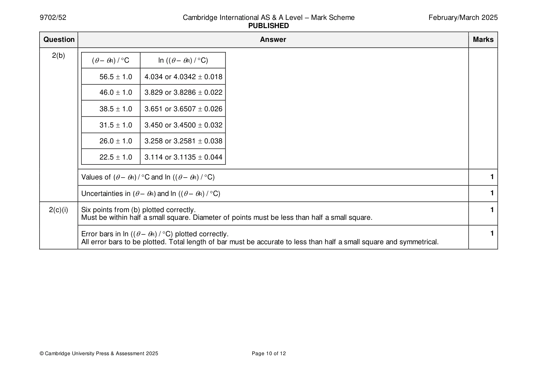
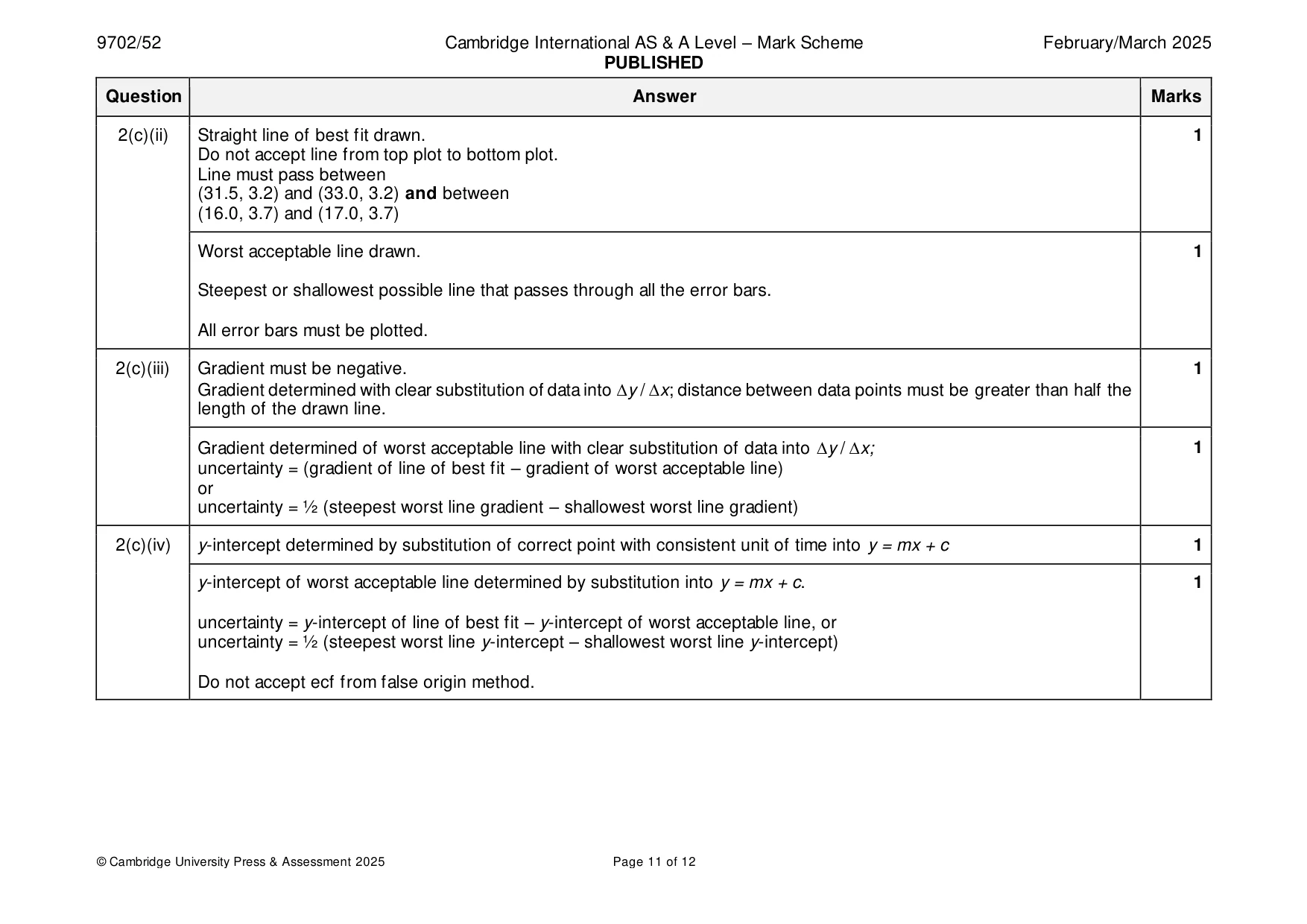
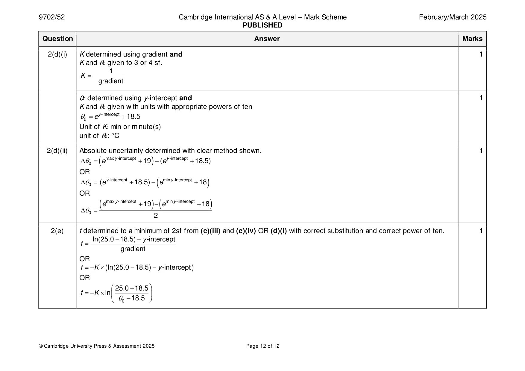
Mark scheme: 2(a) 1 1 gradient = − K y-intercept = ln (0 − R ) 2(b) (– R) / C ln ((– R) / C) 56.5  1.0 4.034 or 4.0342  0.018 46.0  1.0 3.829 or 3.8286  0.022 38.5  1.0 3.651 or 3.6507  0.026 31.5  1.0 3.450 or 3.4500  0.032 26.0  1.0 3.258 or 3.2581  0.038 22.5  1.0 3.114 or 3.1135  0.044 Values of (– R) / C and ln ((– R) / C) 1 Uncertainties in (– R) and ln ((– R) / C) 1 2(c)(i) Six points from (b) plotted correctly. 1 Must be within half a small square. Diameter of points must be less than half a small square. Error bars in ln ((– R) / C) plotted correctly. 1 All error bars to be plotted. Total length of bar must be accurate to less than half a small square and symmetrical. 2(c)(ii) Straight line of best fit drawn. 1 Do not accept line from top plot to bottom plot. Line must pass between (31.5, 3.2) and (33.0, 3.2) and between (16.0, 3.7) and (17.0, 3.7) Worst acceptable line drawn. 1 Steepest or shallowest possible line that passes through all the error bars. All error bars must be plotted. 2(c)(iii) Gradient must be negative. 1 Gradient determined with clear substitution of data into y / x; distance between data points must be greater than half the length of the drawn line. Gradient determined of worst acceptable line with clear substitution of data into y / x; 1 uncertainty = (gradient of line of best fit – gradient of worst acceptable line) or uncertainty = ½ (steepest worst line gradient – shallowest worst line gradient) 2(c)(iv) y-intercept determined by substitution of correct point with consistent unit of time into y = mx + c 1 y-intercept of worst acceptable line determined by substitution into y = mx + c. 1 uncertainty = y-intercept of line of best fit – y-intercept of worst acceptable line, or uncertainty = ½ (steepest worst line y-intercept – shallowest worst line y-intercept) Do not accept ecf from false origin method. 2(d)(i) K determined using gradient and 1 K and 0 given to 3 or 4 sf. 1 K = − gradient 0 determined using y-intercept and 1 K and 0 given with units with appropriate powers of ten =0 e y -intercept + 18.5 Unit of K: min or minute(s) unit of 0: C 2(d)(ii) Absolute uncertainty determined with clear method shown. 1 emax y -intercept + 19 − (e y -intercept + 18.5) 0 = ( ) OR emin y -intercept + 18 0 = (e y -intercept + 18.5) − ( ) OR emax y -intercept + 19 − emin y -intercept + 18 ( ) ( ) 0 = 2 2(e) t determined to a minimum of 2sf from (c)(iii) and (c)(iv) OR (d)(i) with correct substitution and correct power of ten. 1 ln(25.0 − 18.5) − y -intercept t = gradient OR t = − K  ( ln(25.0 − 18.5) − y -intercept ) OR  25.0 − 18.5  t = −K  ln    0 − 18.5 

More questions on Errors and uncertainties