Questions as text
Q1 · 100 students were each asked how much money, $m, they spent in one week 0980/42 May/June 2019
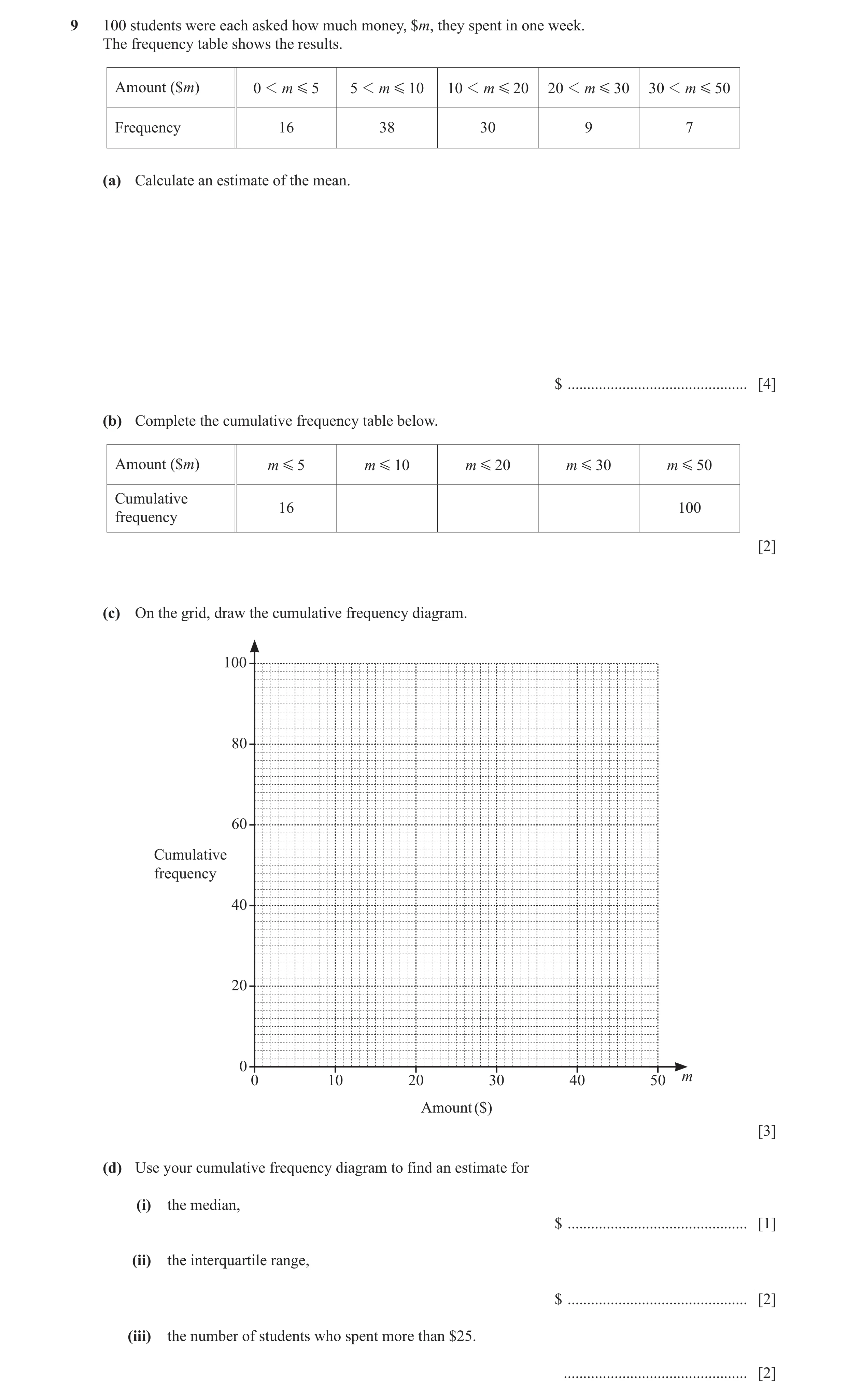
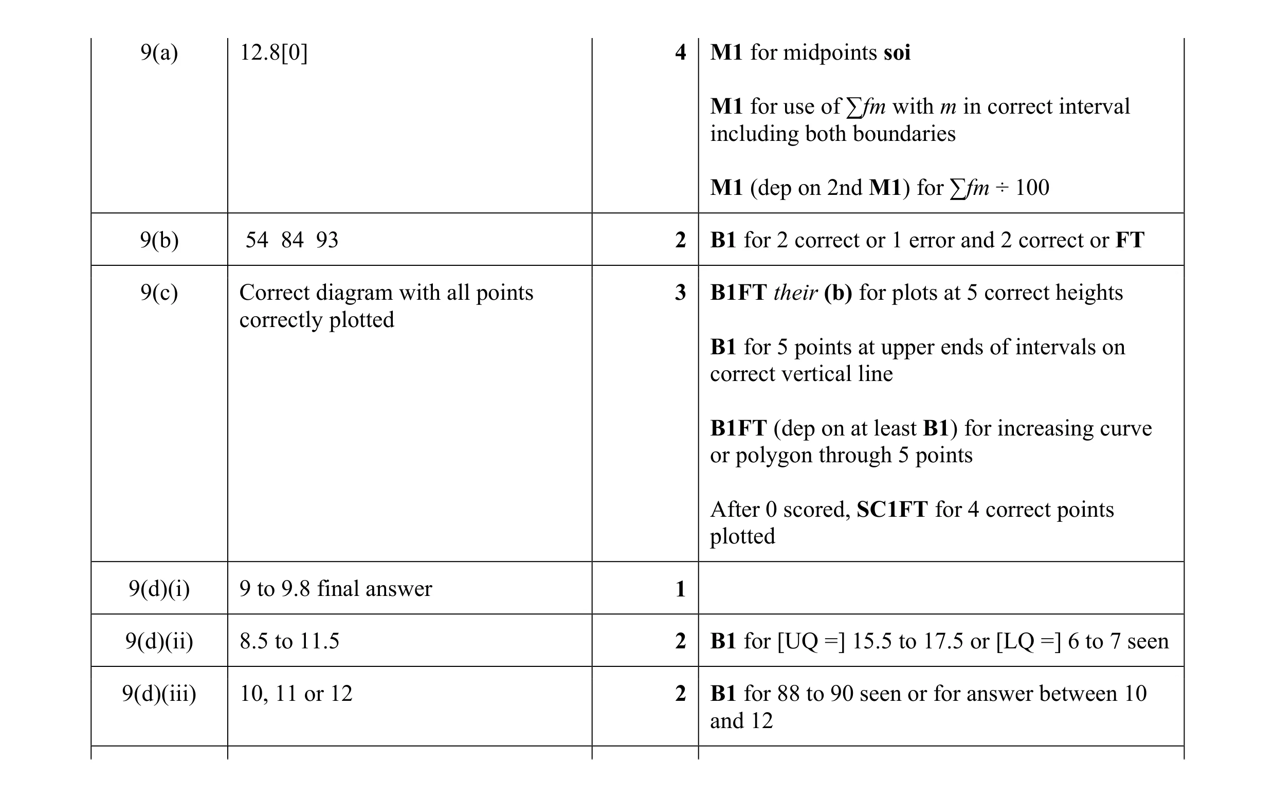
9 100 students were each asked how much money, $m, they spent in one week. The frequency table shows the results. Amount ($m) 0 1 m G 5 5 1 m G 10 10 1 m G 20 20 1 m G 30 30 1 m G 50 Frequency 16 38 30 9 7 (a) Calculate an estimate of the mean. $ … [4] (b) Complete the cumulative frequency table below. Amount ($m) m G 5 m G 10 m G 20 m G 30 m G 50 Cumulative 16 100 frequency [2] (c) On the grid, draw the cumulative frequency diagram. 100 80 60 Cumulative frequency 40 20 0 0 10 20 30 40 50 m Amount ($) [3] (d) Use your cumulative frequency diagram to find an estimate for (i) the median, $ … [1] (ii) the interquartile range, $ … [2] (iii) the number of students who spent more than $25. … [2]
14 marks
Mark scheme: 9(a) 12.8[0] 4 M1 for midpoints soi M1 for use of ∑fm with m in correct interval including both boundaries M1 (dep on 2nd M1) for ∑fm ÷ 100 9(b) 54 84 93 2 B1 for 2 correct or 1 error and 2 correct or FT 9(c) Correct diagram with all points 3 B1FT their (b) for plots at 5 correct heights correctly plotted B1 for 5 points at upper ends of intervals on correct vertical line B1FT (dep on at least B1) for increasing curve or polygon through 5 points After 0 scored, SC1FT for 4 correct points plotted 9(d)(i) 9 to 9.8 final answer 1 9(d)(ii) 8.5 to 11.5 2 B1 for [UQ =] 15.5 to 17.5 or [LQ =] 6 to 7 seen 9(d)(iii) 10, 11 or 12 2 B1 for 88 to 90 seen or for answer between 10 and 12
This question in 0980/42 May/June 2019
Q2 · The cumulative frequency diagram shows information about the times taken by 200 students… 0980/41 Oct/Nov 2019
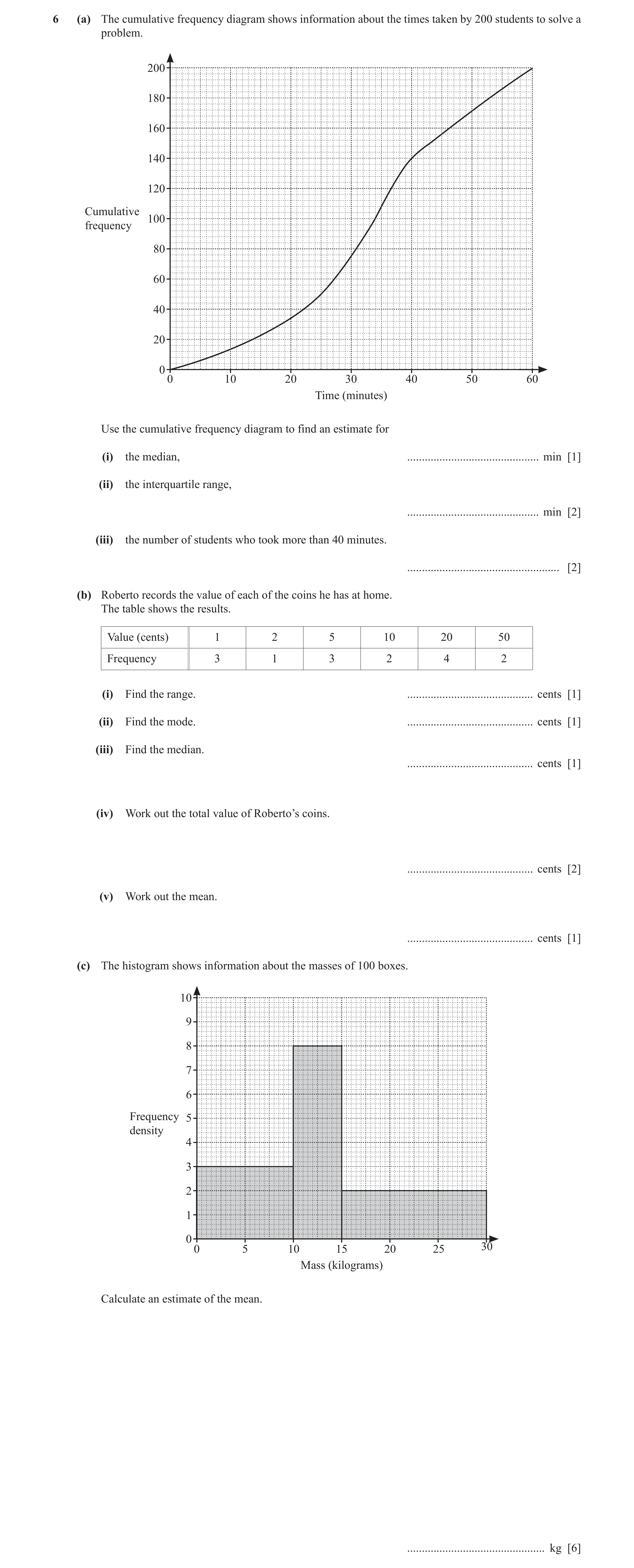
6 (a) The cumulative frequency diagram shows information about the times taken by 200 students to solve a problem. 200 180 160 140 120 Cumulative 100 frequency 80 60 40 20 0 0 10 20 30 40 50 60 Time (minutes) Use the cumulative frequency diagram to find an estimate for (i) the median, … min [1] (ii) the interquartile range, … min [2] (iii) the number of students who took more than 40 minutes. … [2] (b) Roberto records the value of each of the coins he has at home. The table shows the results. Value (cents) 1 2 5 10 20 50 Frequency 3 1 3 2 4 2 (i) Find the range. … cents [1] (ii) Find the mode. … cents [1] (iii) Find the median. … cents [1] (iv) Work out the total value of Roberto’s coins. … cents [2] (v) Work out the mean. … cents [1] (c) The histogram shows information about the masses of 100 boxes. 10 9 8 7 6 Frequency 5 density 4 3 2 1 0 0 5 10 15 20 25 30 Mass (kilograms) Calculate an estimate of the mean. … kg [6]
17 marks
Mark scheme: 6(a)(i) 34 1 6(a)(ii) 18 2 B1 for [l.q. = ] 25 or [u.q. = ] 43 seen 6(a)(iii) 60 2 M1 for 140 written 6(b)(i) 49 1 6(b)(ii) 20 1 6(b)(iii) 10 1 6(b)(iv) 220 2 M1 for 3 × 1 + 1 × 2 + 3 × 5 + 2 × 10 + 4 × 20 + 2 × 50 6(b)(v) 14.7 or 14.66 to 14.67 1 FT their (iv) ÷ 15 6(c) 13.25 nfww 6 B2 for frequencies 30, 40, 30 soi or B1 for 2 of these M1 for 5, 12.5, 22.5 M1 Σfx with their frequencies (if seen) and each x in correct interval including boundaries Σfx M1 dependent for (dependent on 100 second M1) OR Alternative Method B2 for frequencies 15, 15, 40, 10, 10, 10 soi or B1 for 2 of 15, 40, 10 M1 for 2.5, 7.5, 12.5, 17.5, 22.5, 27.5 M1 Σfx with their frequencies (if seen) and each x in correct interval including boundaries Σfx M1 dependent for (dependent on 100 second M1)
This question in 0980/41 Oct/Nov 2019
Q3 · The speed, v km/h, of each of 200 cars passing a building is measured 0980/42 May/June 2020
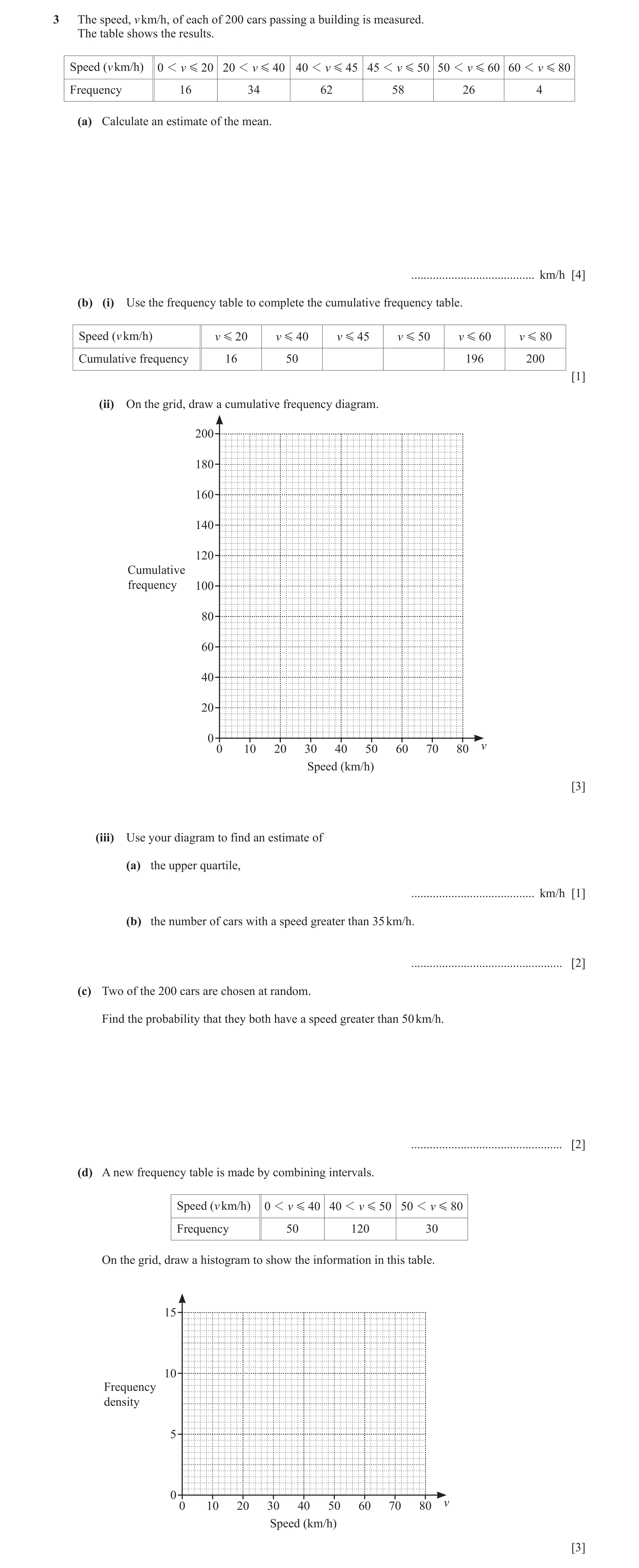
3 The speed, v km/h, of each of 200 cars passing a building is measured. The table shows the results. Speed (v km/h) 0 1 v G 20 20 1 v G 40 40 1 v G 45 45 1 v G 50 50 1 v G 60 60 1 v G 80 Frequency 16 34 62 58 26 4 (a) Calculate an estimate of the mean. … km/h [4] (b) (i) Use the frequency table to complete the cumulative frequency table. Speed (v km/h) v G 20 v G 40 v G 45 v G 50 v G 60 v G 80 Cumulative frequency 16 50 196 200 [1] (ii) On the grid, draw a cumulative frequency diagram. 200 180 160 140 120 Cumulative frequency 100 80 60 40 20 0 v 0 10 20 30 40 50 60 70 80 Speed (km/h) [3] (iii) Use your diagram to find an estimate of (a) the upper quartile, … km/h [1] (b) the number of cars with a speed greater than 35 km/h. … [2] (c) Two of the 200 cars are chosen at random. Find the probability that they both have a speed greater than 50 km/h. … [2] (d) A new frequency table is made by combining intervals. Speed (v km/h) 0 1 v G 40 40 1 v G 50 50 1 v G 80 Frequency 50 120 30 On the grid, draw a histogram to show the information in this table. 15 10 Frequency density 5 0 v 0 10 20 30 40 50 60 70 80 Speed (km/h) [3]
16 marks
Mark scheme: 3(a) 41.4 4 M1 for 10, 30, 42.5, 47.5, 55, 70 M1 for Σ fx where x lies in or on the boundary of each interval. Σfx M1 dep for dep on second M1 200 3(b)(i) 112, 170 1 3(b)(ii) Correct diagram 3 B1 for correct horizontal plot B1FT for correct vertical plots B1 FT dep on at least B1 earned for reasonable increasing curve or polygon through their 6 points If 0 scored SC1FT for 5 out of 6 points plotted correctly 3(b)(iii)(a) 48 1 3(b)(iii)(b) 160 2 M1 for 40 seen 3(c) 87 2 30 29 oe M1 for × oe 3980 200 199 3(d) Correct histogram 3 B1 for each column If 0 scored SC1 for correct frequency densities soi 1.25, 12, 1
This question in 0980/42 May/June 2020
Q4 · Women Men 0 60 120 180 240 300 360 420 Time (minutes) The box-and-whisker plots show the… 0980/41 Oct/Nov 2020
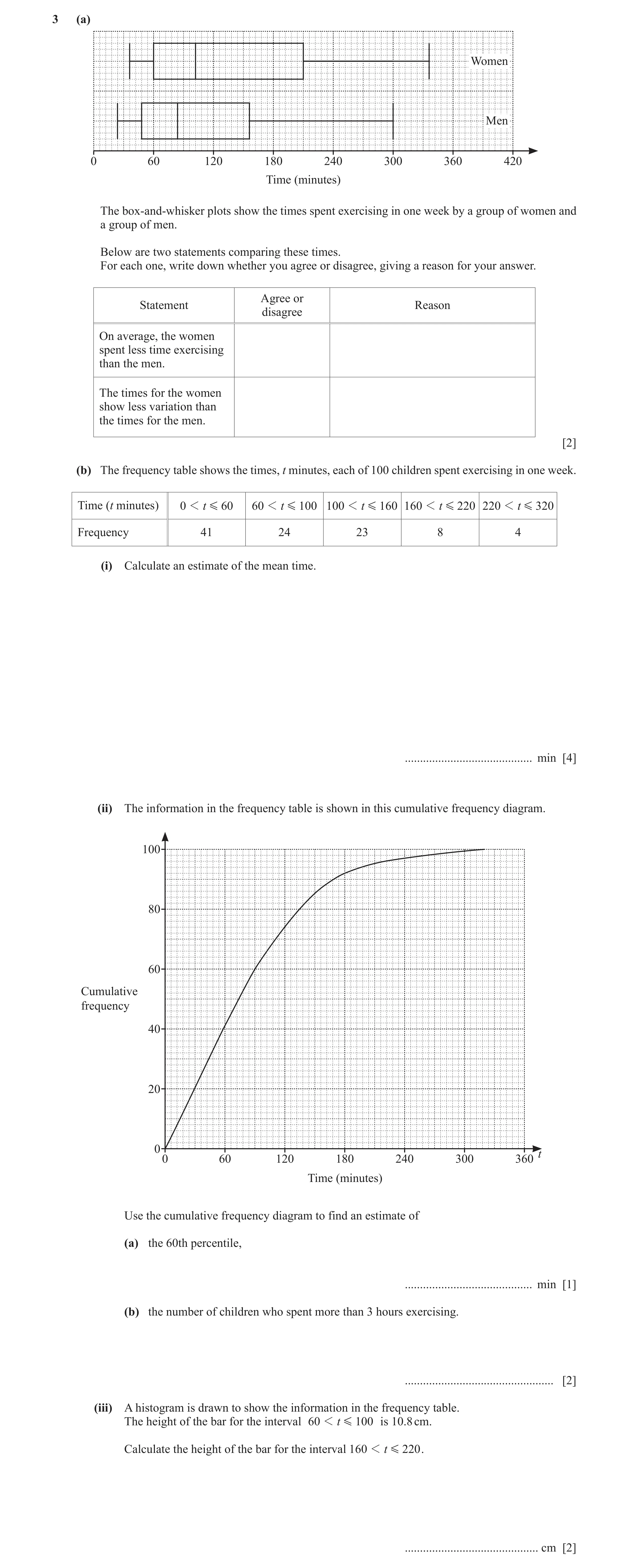
3 (a) Women Men 0 60 120 180 240 300 360 420 Time (minutes) The box-and-whisker plots show the times spent exercising in one week by a group of women and a group of men. Below are two statements comparing these times. For each one, write down whether you agree or disagree, giving a reason for your answer. Agree or Statement Reason disagree On average, the women spent less time exercising than the men. The times for the women show less variation than the times for the men. [2] (b) The frequency table shows the times, t minutes, each of 100 children spent exercising in one week. Time (t minutes) 0 1 t G 60 60 1 t G 100 100 1 t G 160 160 1 t G 220 220 1 t G 320 Frequency 41 24 23 8 4 (i) Calculate an estimate of the mean time. … min [4] (ii) The information in the frequency table is shown in this cumulative frequency diagram. 100 80 60 Cumulative frequency 40 20 0 t 0 60 120 180 240 300 360 Time (minutes) Use the cumulative frequency diagram to find an estimate of (a) the 60th percentile, … min [1] (b) the number of children who spent more than 3 hours exercising. … [2] (iii) A histogram is drawn to show the information in the frequency table. The height of the bar for the interval 60 1 t G 100 is 10.8 cm. Calculate the height of the bar for the interval 160 1 t G 220 . … cm [2]
11 marks
Mark scheme: 3(a) Disagree: the median for the women is 2 B1 for each correct statement oe greater (than the median for the men) oe Disagree: the men have a smaller [interquartile] range of times oe 3(b)(i) 87.4 nfww 4 M1 for mid-points soi (30, 80, 130, 190, 270) M1 for use of Σfm with m in correct interval including both boundaries M1 (dep on 2nd M1) for Σfm ÷ (41 + 24 + 23 + 8 + 4) 3(b)(ii)(a) 90 1 3(b)(ii)(b) 8 2 B1 for 92 seen 3(b)(iii) 2.4 2 24 8 M1 for or 40 60 1 Or B1 for [multiplier] 18 or 18
This question in 0980/41 Oct/Nov 2020
Q5 · The mass, m kg, of each of 40 parcels in a warehouse is recorded 0980/42 May/June 2021
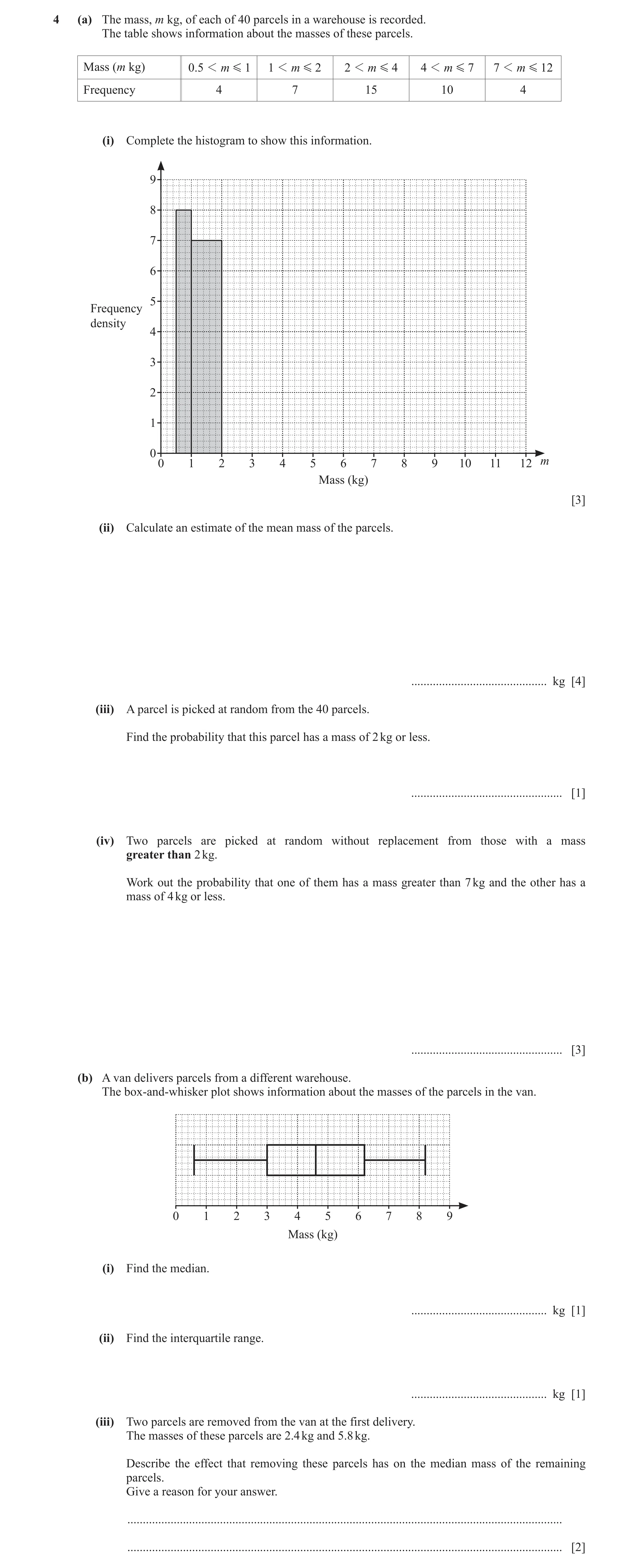
4 (a) The mass, m kg, of each of 40 parcels in a warehouse is recorded. The table shows information about the masses of these parcels. Mass (m kg) 0.5 1 m G 1 1 1 m G 2 2 1 m G 4 4 1 m G 7 7 1 m G 12 Frequency 4 7 15 10 4 (i) Complete the histogram to show this information. 9 8 7 6 5 Frequency density 4 3 2 1 0 0 1 2 3 4 5 6 7 8 9 10 11 12 m Mass (kg) [3] (ii) Calculate an estimate of the mean mass of the parcels. … kg [4] (iii) A parcel is picked at random from the 40 parcels. Find the probability that this parcel has a mass of 2 kg or less. … [1] (iv) Two parcels are picked at random without replacement from those with a mass greater than 2 kg. Work out the probability that one of them has a mass greater than 7 kg and the other has a mass of 4 kg or less. … [3] (b) A van delivers parcels from a different warehouse. The box-and-whisker plot shows information about the masses of the parcels in the van. 0 1 2 3 4 5 6 7 8 9 Mass (kg) (i) Find the median. … kg [1] (ii) Find the interquartile range. … kg [1] (iii) Two parcels are removed from the van at the first delivery. The masses of these parcels are 2.4 kg and 5.8 kg. Describe the effect that removing these parcels has on the median mass of the remaining parcels. Give a reason for your answer. … … [2]
15 marks
Mark scheme: 4(a)(i) Correct histogram 3 B1 for each correct block If 0 scored, SC1 for any two of fds 7.5, 3.33…, 0.8 oe soi 4(a)(ii) 3.7875 or 3.79 or 3.787 or 3.788 4 M1 for 0.75, 1.5, 3, 5.5, 9.5 soi M1 for Σ fx M1 dep for their Σ fx ÷ 40 4(a)(iii) 11 1 oe 40 4(a)(iv) 30 3 4 15 oe M2 for [2 ×] × oe 203 29 28 4 15 or M1 for or oe seen 29 29 4 26 After 0 scored, SC1 for [ 2 × ] × 40 39 oe 120 or for answer oe 841 4(b)(i) 4.6 1 4(b)(ii) 3.2 1 4(b)(iii) [median] remains the same oe 2 B1 for each statement and one is below [the median/middle] and one is above oe
This question in 0980/42 May/June 2021
Q6 · The cumulative frequency diagram shows information about the mass, m kg, of each of 80… 0980/41 Oct/Nov 2021
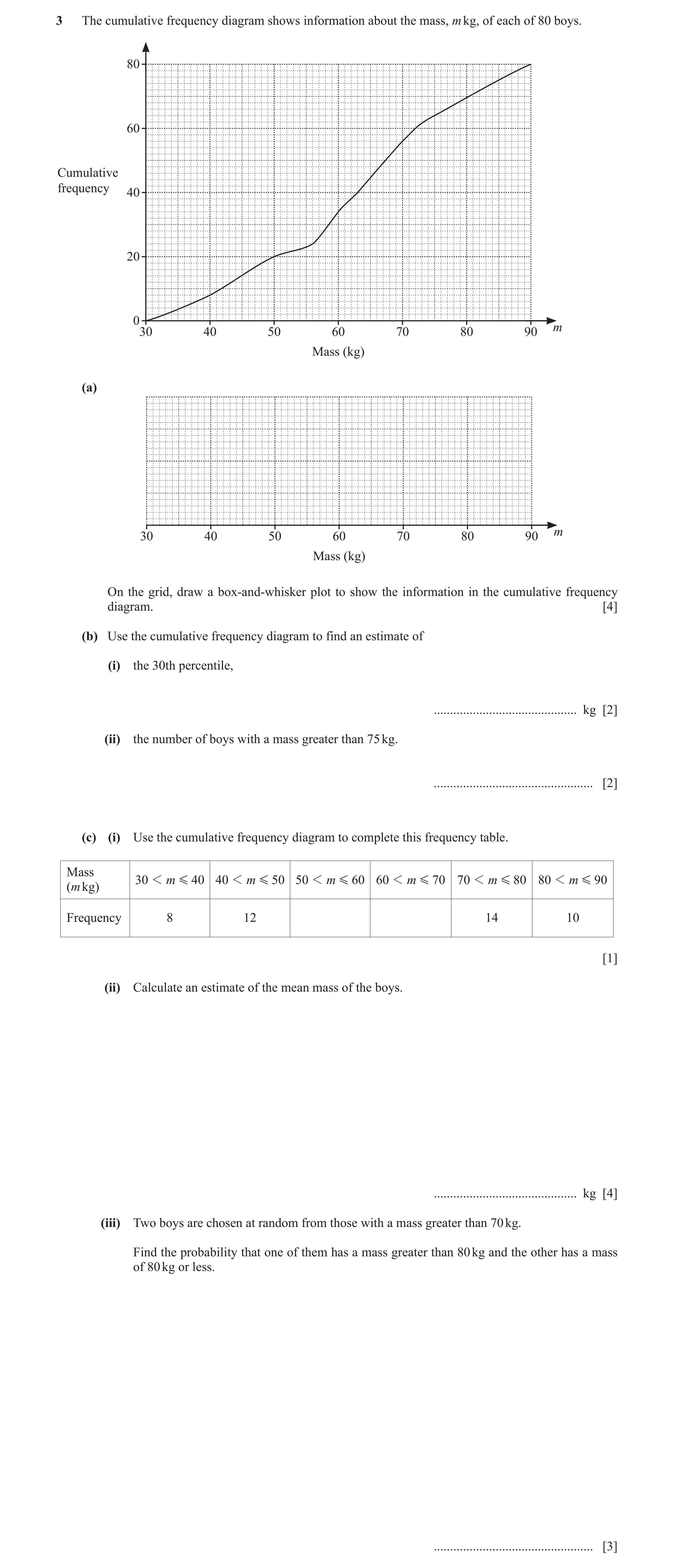
3 The cumulative frequency diagram shows information about the mass, m kg, of each of 80 boys. 80 60 Cumulative frequency 40 20 0 m 30 40 50 60 70 80 90 Mass (kg) (a) m 30 40 50 60 70 80 90 Mass (kg) On the grid, draw a box-and-whisker plot to show the information in the cumulative frequency diagram. [4] (b) Use the cumulative frequency diagram to find an estimate of (i) the 30th percentile, … kg [2] (ii) the number of boys with a mass greater than 75 kg. … [2] (c) (i) Use the cumulative frequency diagram to complete this frequency table. Mass 30 1 m G 40 40 1 m G 50 50 1 m G 60 60 1 m G 70 70 1 m G 80 80 1 m G 90(m kg) Frequency 8 12 14 10 [1] (ii) Calculate an estimate of the mean mass of the boys. … kg [4] (iii) Two boys are chosen at random from those with a mass greater than 70 kg. Find the probability that one of them has a mass greater than 80 kg and the other has a mass of 80 kg or less. … [3]
16 marks
Mark scheme: 3(a) Correct box-and-whisker plot 4 B1 for lowest value and highest value at 30 and 90 B1 for LQ and UQ at 50 and 72 B1 for median at 63 3(b)(i) 56 2 M1 for 24 soi 3(b)(ii) 16 2 B1 for 64 written 3(c)(i) 14, 22 1 3(c)(ii) 61.5 4 M1 for 35, 45, 55, 65, 75, 85 soi M1 for Σ fx M1 dep for their Σ fx ÷ (8 + 12 +their 14 + their 22 + 14 +10) or Σ fx ÷ 80 3(c)(iii) 35 3 10 14 oe M2 for [2] × oe 69 24 23 10 14 or M1 for or oe seen 24 24 35 If 0 scored, SC1 for answer oe 72
This question in 0980/41 Oct/Nov 2021
Q7 · Information about the mass, m kg, of each of 150 children is recorded in the frequency… 0980/42 May/June 2022
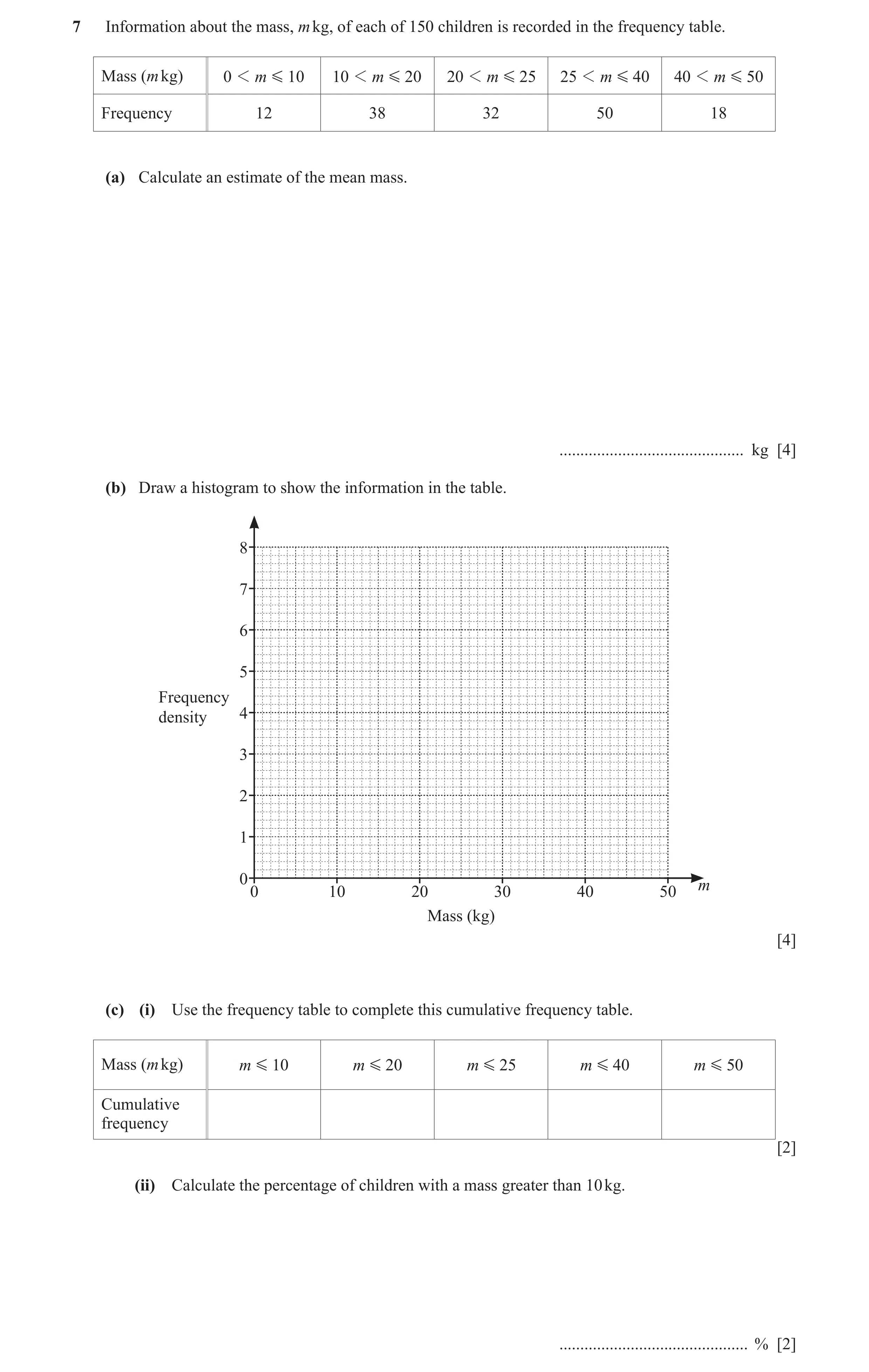
7 Information about the mass, m kg, of each of 150 children is recorded in the frequency table. Mass (m kg) 0 1 m G 10 10 1 m G 20 20 1 m G 25 25 1 m G 40 40 1 m G 50 Frequency 12 38 32 50 18 (a) Calculate an estimate of the mean mass. … kg [4] (b) Draw a histogram to show the information in the table. 8 7 6 5 Frequency density 4 3 2 1 0 m 0 10 20 30 40 50 Mass (kg) [4] (c) (i) Use the frequency table to complete this cumulative frequency table. Mass (m kg) m G 10 m G 20 m G 25 m G 40 m G 50 Cumulative frequency [2] (ii) Calculate the percentage of children with a mass greater than 10 kg. … % [2]
12 marks
Mark scheme: 7(a) 25.2 or 25.23… 4 M1 for midpoints soi M1 for use of ∑fx with x in correct interval including both boundaries M1 (dep on 2nd M1) for ∑fx ÷ 150 7(b) 5 correct blocks 4 B3 for 4 correct blocks or B2 for 3 correct blocks or B1 for 2 correct blocks or block widths 10, 10, 5, 15, 10 If 0 scored SC1 for 4 correct frequency densities from 1.2, 3.8, 6.4, 3.33[3…] and 1.8 oe soi 7(c)(i) 12, 50, 82, 132, 150 2 B1 for 3 or 4 correct 7(c)(ii) 92 2 M1 for 150 −12 oe seen If 0 scored, SC1 for answer 8[%]
This question in 0980/42 May/June 2022
Q8 · 100 students each record the time, t minutes, taken to eat a pizza 0980/41 Oct/Nov 2022
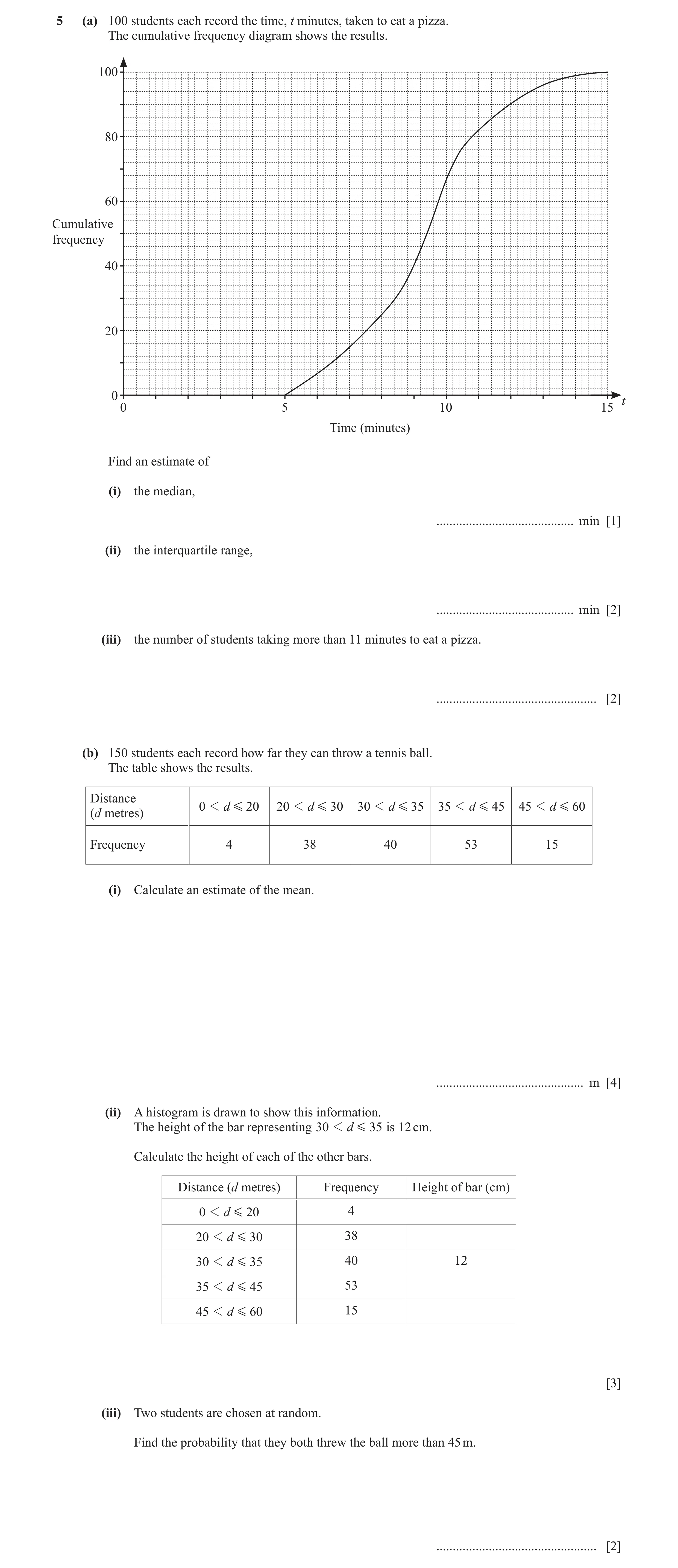
5 (a) 100 students each record the time, t minutes, taken to eat a pizza. The cumulative frequency diagram shows the results. 100 80 60 Cumulative frequency 40 20 0 t 0 5 10 15 Time (minutes) Find an estimate of (i) the median, … min [1] (ii) the interquartile range, … min [2] (iii) the number of students taking more than 11 minutes to eat a pizza. … [2] (b) 150 students each record how far they can throw a tennis ball. The table shows the results. Distance 0 1 d G 20 20 1 d G 30 30 1 d G 35 35 1 d G 45 45 1 d G 60 (d metres) Frequency 4 38 40 53 15 (i) Calculate an estimate of the mean. … m [4] (ii) A histogram is drawn to show this information. The height of the bar representing 30 1 d G 35 is 12 cm. Calculate the height of each of the other bars. Distance (d metres) Frequency Height of bar (cm) 0 1 d G 20 4 20 1 d G 30 38 30 1 d G 35 40 12 35 1 d G 45 53 45 1 d G 60 15 [3] (iii) Two students are chosen at random. Find the probability that they both threw the ball more than 45 m. … [2]
14 marks
Mark scheme: 5(a)(i) 9.4 1 5(a)(ii) 2.4 2 B1 for [uq =] 10.4 or [lq =] 8 but not as final answer 5(a)(iii) 18 2 B1 for 82 seen 5(b)(i) 13 4 M1 for midpoints 10, 25, 32.5, 40, 52.5 34.65 or 34 soi 20 M1 for fx where values of x are in interval or on boundary fx M1 dep on second M for 150 5(b)(ii) 0.3, 5.7, ..., 7.95, 1.5 3 B2 for any two correct or B1 for one correct or for at least three frequency densities seen 0.2, 3.8, 8, 5.3, 1 oe or M1 for [factor] 1.5 5(b)(iii) 7 2 15 14 oe M1 for 745 150 149
This question in 0980/41 Oct/Nov 2022
Q9 · The table shows information about the heights of 80 children 0980/42 May/June 2023
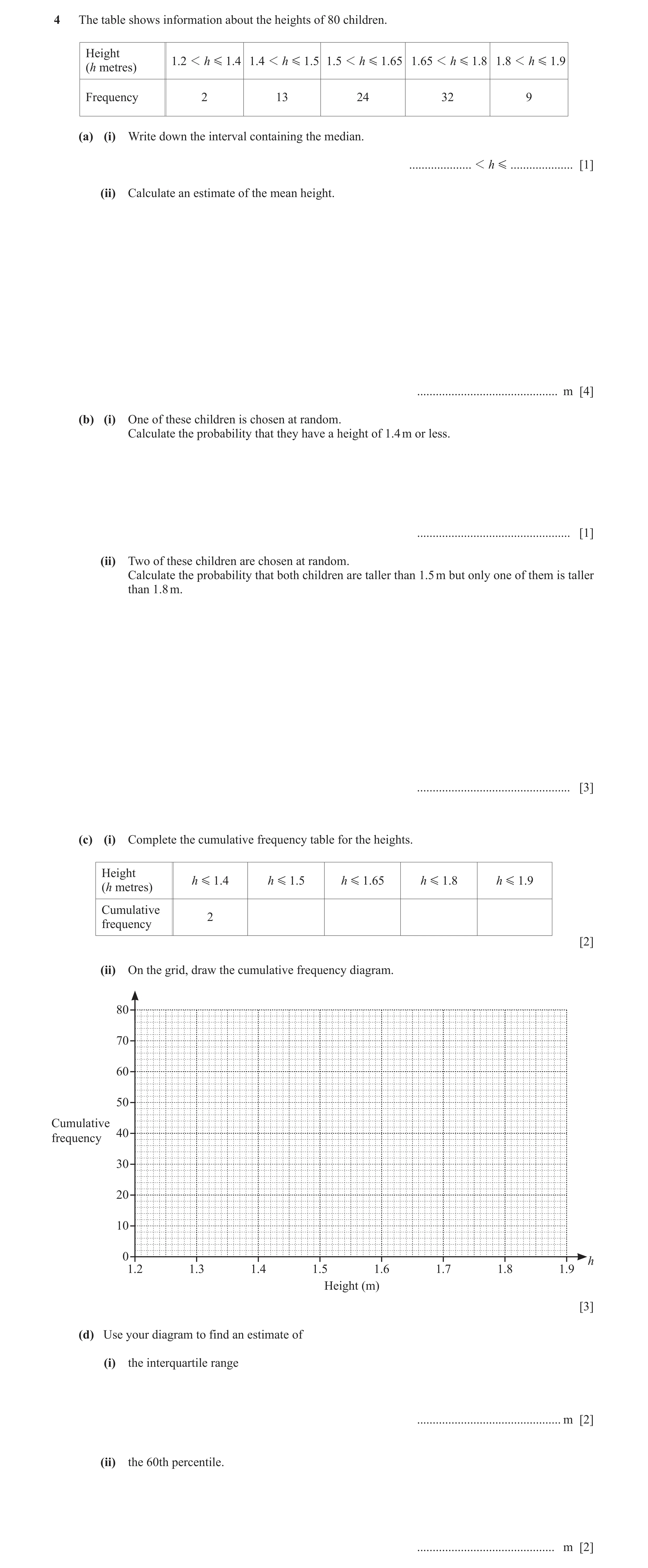
4 The table shows information about the heights of 80 children. Height 1.2 1 h G 1.4 1.4 1 h G 1.5 1.5 1 h G 1.65 1.65 1 h G 1. 8 1.8 1 h G 1.9 (h metres) Frequency 2 13 24 32 9 (a) (i) Write down the interval containing the median. … 1 h G … [1] (ii) Calculate an estimate of the mean height. … m [4] (b) (i) One of these children is chosen at random. Calculate the probability that they have a height of 1.4 m or less. … [1] (ii) Two of these children are chosen at random. Calculate the probability that both children are taller than 1.5 m but only one of them is taller than 1.8 m. … [3] (c) (i) Complete the cumulative frequency table for the heights. Height h G 1.4 h G 1.5 h G 1.65 h G 1.8 h G 1.9 (h metres) Cumulative 2 frequency [2] (ii) On the grid, draw the cumulative frequency diagram. 80 70 60 50 Cumulative 40frequency 30 20 10 0 h 1.2 1.3 1.4 1.5 1.6 1.7 1.8 1.9 Height (m) [3] (d) Use your diagram to find an estimate of (i) the interquartile range … m [2] (ii) the 60th percentile. … m [2]
18 marks
Mark scheme: 4(a)(i) 1.65 < h ≤ 1.8 1 4(a)(ii) 1.63875 4 M1 for midpoints soi M1 for use of ∑fh with h in correct interval including both boundaries M1dep on 2nd M1 for ∑fh ÷ 80 4(b)(i) 1 1 oe 40 4(b)(ii) 63 3 56 9 oe M2 for [ 2] oe 395 80 79 56 9 9 56 or B1 for or or or oe seen 80 79 80 79 If 0 or B1 scored, instead award SC2 for 117 answer oe 632 63 or SC1 for answer oe 400 4(c)(i) 15, 39, 71, 80 2 B1 for 3 correct or M1 for 1 error in addition with other values then consistent 4(c)(ii) Correct curve 3 B1 for correct horizontal placement for 5 plots B1FT for correct vertical placement for 5 plots B1FT dep on at least B1 for reasonable increasing curve or polygon through their 5 points If 0 scored SC1 FT for 4 out of 5 points correctly plotted 4(d)(i) Strict FT their UQ – their LQ 2dep B1dep for their UQ or their LQ seen Dep on increasing curve/polygon for 2 marks or B1 4(d)(ii) Strict FT their reading at 48 2dep B1 for 48 written
This question in 0980/42 May/June 2023
Q10 · The frequency table shows the time of each of 42 athletes in a race 0980/41 Oct/Nov 2023
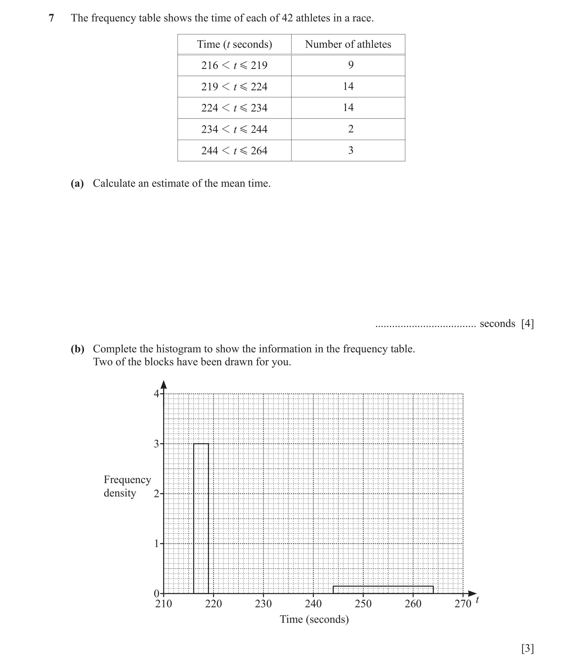
7 The frequency table shows the time of each of 42 athletes in a race. Time (t seconds) Number of athletes 216 1 t G 219 9 219 1 t G 224 14 224 1 t G 234 14 234 1 t G 244 2 244 1 t G 264 3 (a) Calculate an estimate of the mean time. … seconds [4] (b) Complete the histogram to show the information in the frequency table. Two of the blocks have been drawn for you. 4 3 Frequency density 2 1 0 t 210 220 230 240 250 260 270 Time (seconds) [3]
7 marks
Mark scheme: 7(a) 226 nfww or 226.2 to 226.3[0] 4 M1 for mid-points soi nfww (217.5, 221.5, 229, 239, 254) M1 for use of fm with m in correct interval including both boundaries M1 (dep on 2nd M1) for fm (9 + 14 + 14 + 2 + 3) 7(b) Blocks with heights 2.8, 1.4, 0.2 3 B1 for each correct block and with correct widths If 0 scored, SC1 for two correct frequency densities soi
This question in 0980/41 Oct/Nov 2023
Q11 · The table shows the time that each of 40 students takes to travel to school 0980/42 May/June 2024
3 (a) The table shows the time that each of 40 students takes to travel to school. Time (m minutes) 0 1 m G 10 10 1 m G 25 25 1 m G 40 40 1 m G 60 Frequency 3 18 15 4 (i) Calculate an estimate of the mean. … min [4] (ii) On the grid, draw a histogram to show the information in the table. 2 Frequency 1 density 0 m 0 10 20 30 40 50 60 Time (minutes) [3] (iii) Two students are selected at random from the 40 students. Calculate the probability that one student takes more than 25 minutes and the other student takes 10 minutes or less to travel to school. … [3] (b) This is some information about the time that 200 people took to fill in a questionnaire: • The longest time taken was 30 minutes. • The median time was 22 minutes. • The lower quartile was 8 minutes. • The interquartile range was 19 minutes. • The range was 25 minutes. (i) Write down the shortest time taken. … minutes [1] (ii) On the grid, draw a box-and-whisker plot to show this information. 0 10 20 30 40 Time (minutes) [3] (iii) George says that 101 of the 200 people took more than 22 minutes to fill in the questionnaire. Explain why he is wrong. … [1]
15 marks
Mark scheme: 3(a)(i) 25.4375 4 M1 for mid-points soi (5, 17.5, 32.5, 50) M1 for use of fm with m in correct interval including both boundaries M1 for (dep on 2nd M1) for fm 40 3(a)(ii) correct histogram 3 B2 for 3 correct blocks or B1 for 2 correct blocks If 0 scored SC1 for 4 correct frequency densities 0.3, 1.2, 1, 0.2 oe soi 3(a)(iii) 19 3 oe 260 19 3 M2 for 2 oe 40 39 19 3 19 3 or M1 for any of , , , oe 40 40 39 39 seen 57 If 0 scored, SC1 for oe 800 3(b)(i) 5 1 3(b)(ii) 3 5 30 B2 for with LQ at 8 and median at 22 and 8 22 27 UQ at 27 and boxed or M1 for LQ at 8 and median at 22 Correct box plot or for UQ at 27 B1 for lowest = 5 and highest = 30 Max B1 if not box and whisker diagram 3(b)(iii) Correct explanation which states the 1 median is 22 and correct reference to 100 or 101 e.g. Median is 22 which is 50% of the people and 101 is more than 50% oe The median is 22 which is the 100th number (accept 100.5th number)
This question in 0980/42 May/June 2024
Q12 · The table shows the waiting times for 120 patients at a medical centre 0980/41 Oct/Nov 2024
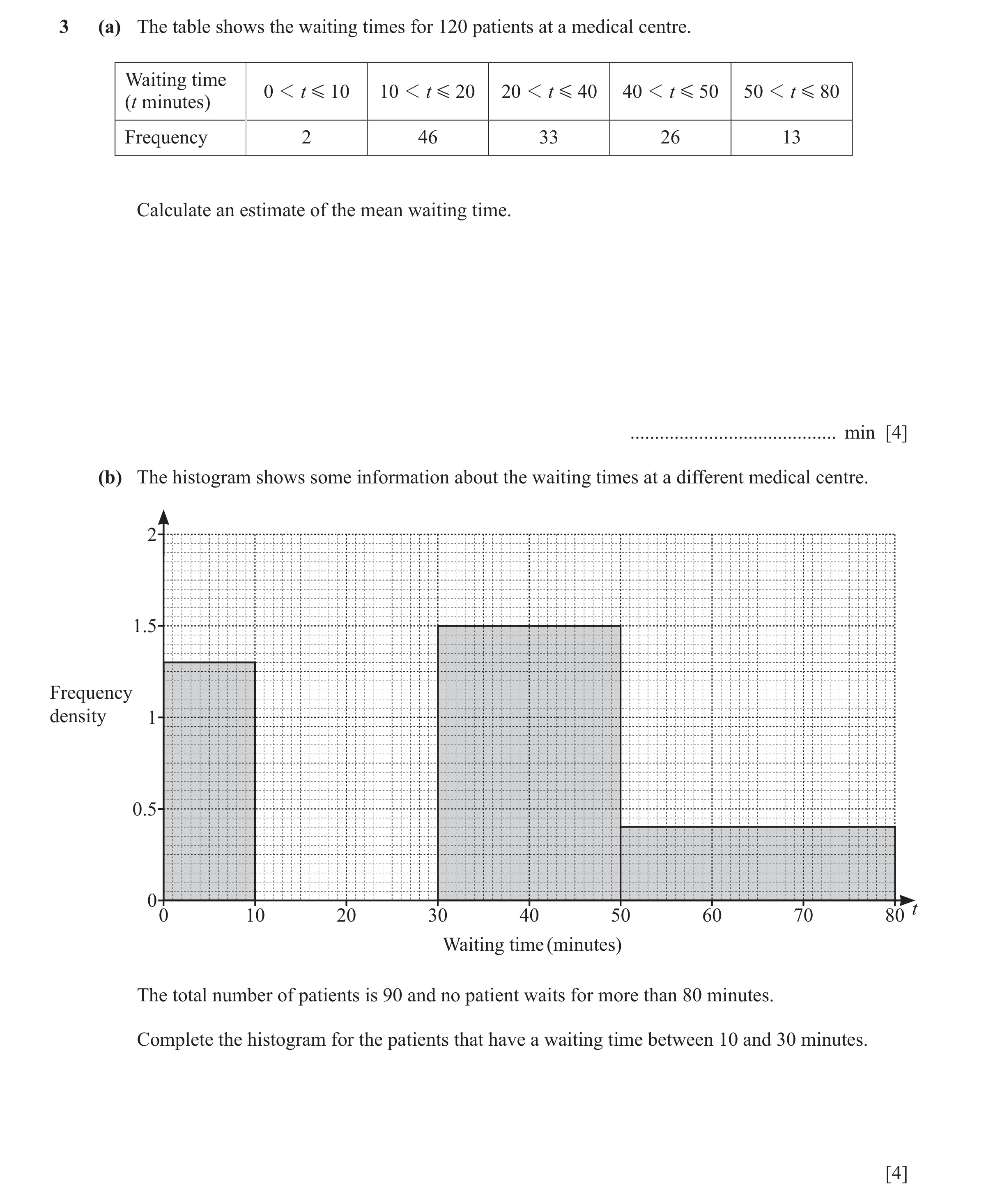
3 (a) The table shows the waiting times for 120 patients at a medical centre. Waiting time 0 1 t G 10 10 1 t G 20 20 1 t G 40 40 1 t G 50 50 1 t G 80 (t minutes) Frequency 2 46 33 26 13 Calculate an estimate of the mean waiting time. … min [4] (b) The histogram shows some information about the waiting times at a different medical centre. 2 1.5 Frequency density 1 0.5 0 t 0 10 20 30 40 50 60 70 80 Waiting time (minutes) The total number of patients is 90 and no patient waits for more than 80 minutes. Complete the histogram for the patients that have a waiting time between 10 and 30 minutes. [4]
8 marks
Mark scheme: 3(a) 30.875 4 M1 for 5, 15, 30, 45, 65 soi M1 for fx M1 dep for their fx ÷ 120 dep on 2nd M1 3(b) Draws correct bar to height 1.75 4 B3 for [height = ] 1.75 OR M2 for [90 – ](10 × 1.3 + 20 × 1.5 + 30 × 0.4) oe or M1 for 10 × 1.3 or 20 × 1.5 or 30 × 0.4 M1dep for their frequency ÷ 20 dep on at least M1 After 0 scored SC1 for bar of correct width and height between 1.7 and 1.8
This question in 0980/41 Oct/Nov 2024
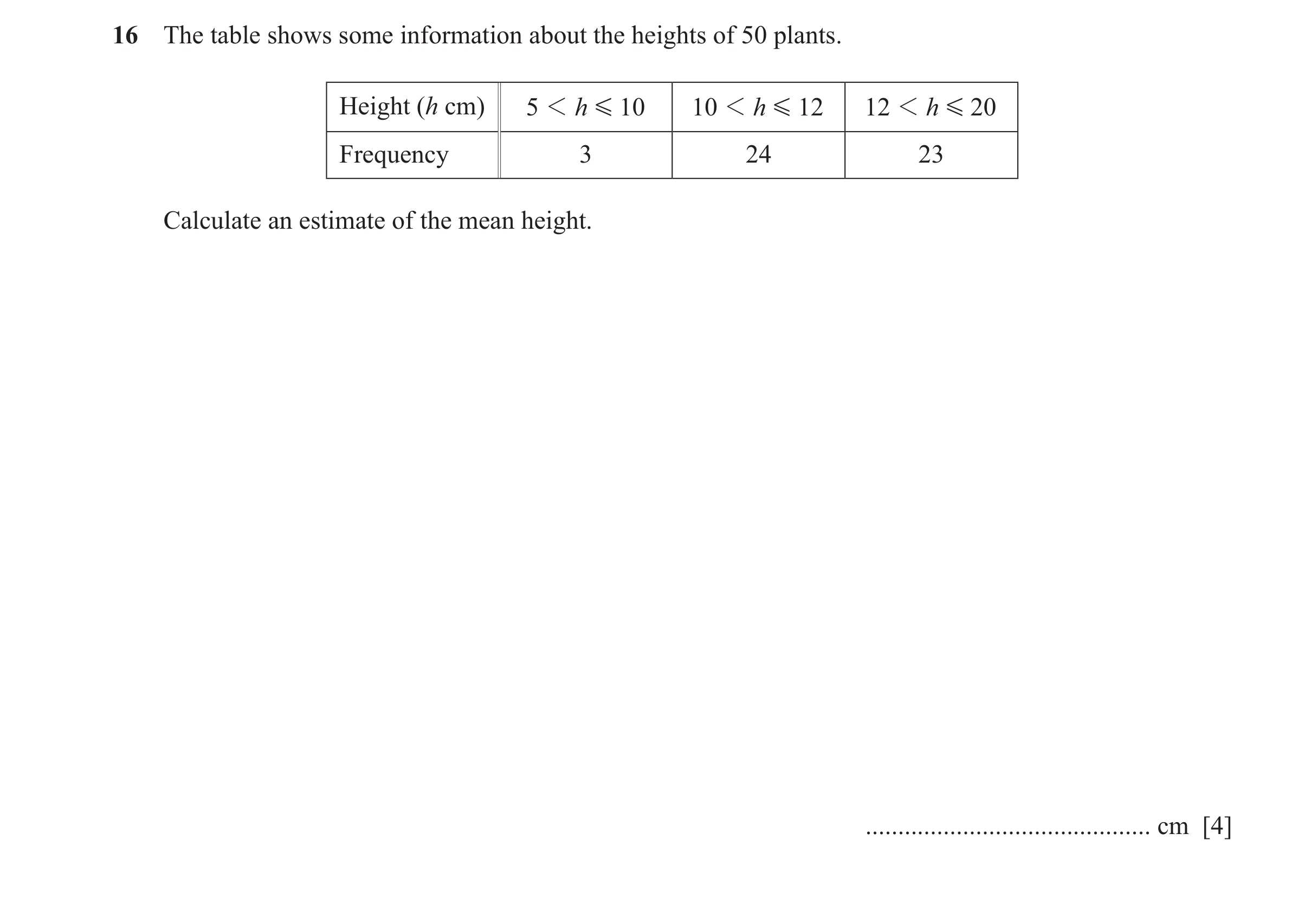
Q13 · The table shows some information about the heights of 50 plants 0980/41 Oct/Nov 2025
16 The table shows some information about the heights of 50 plants. Height (h cm) 5 1 h G 10 10 1 h G 12 12 1 h G 20 Frequency 3 24 23 Calculate an estimate of the mean height. … cm [4]
4 marks
Mark scheme: 16 13.09 4 M1 for mid-values 7.5, 11 and 16 soi M1 for fx where x-values in correct interval (including boundaries) fx M1dep on second M1 for 50
This question in 0980/41 Oct/Nov 2025
 17 / 21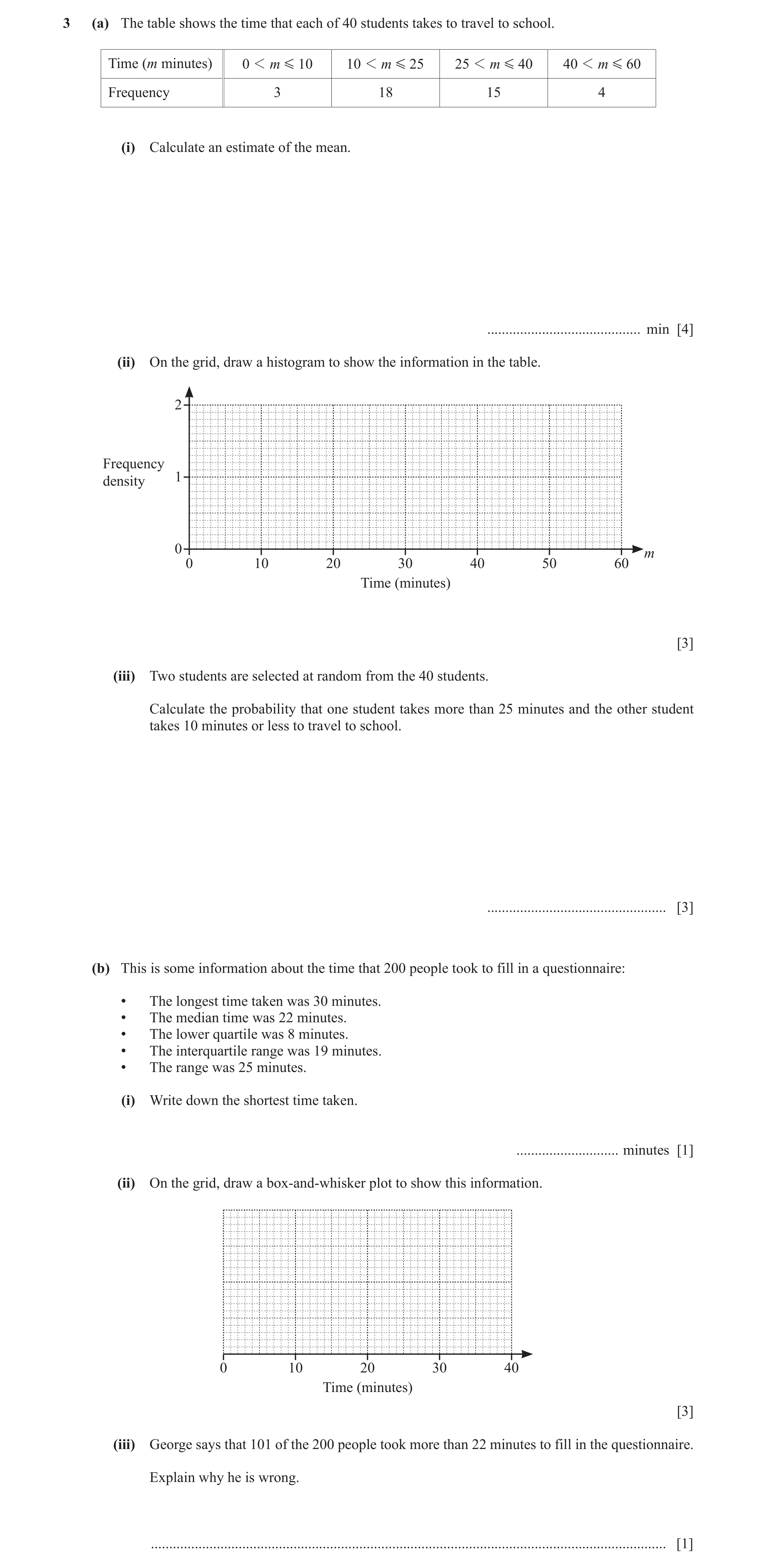
 20 / 21
 21 / 21
 14
14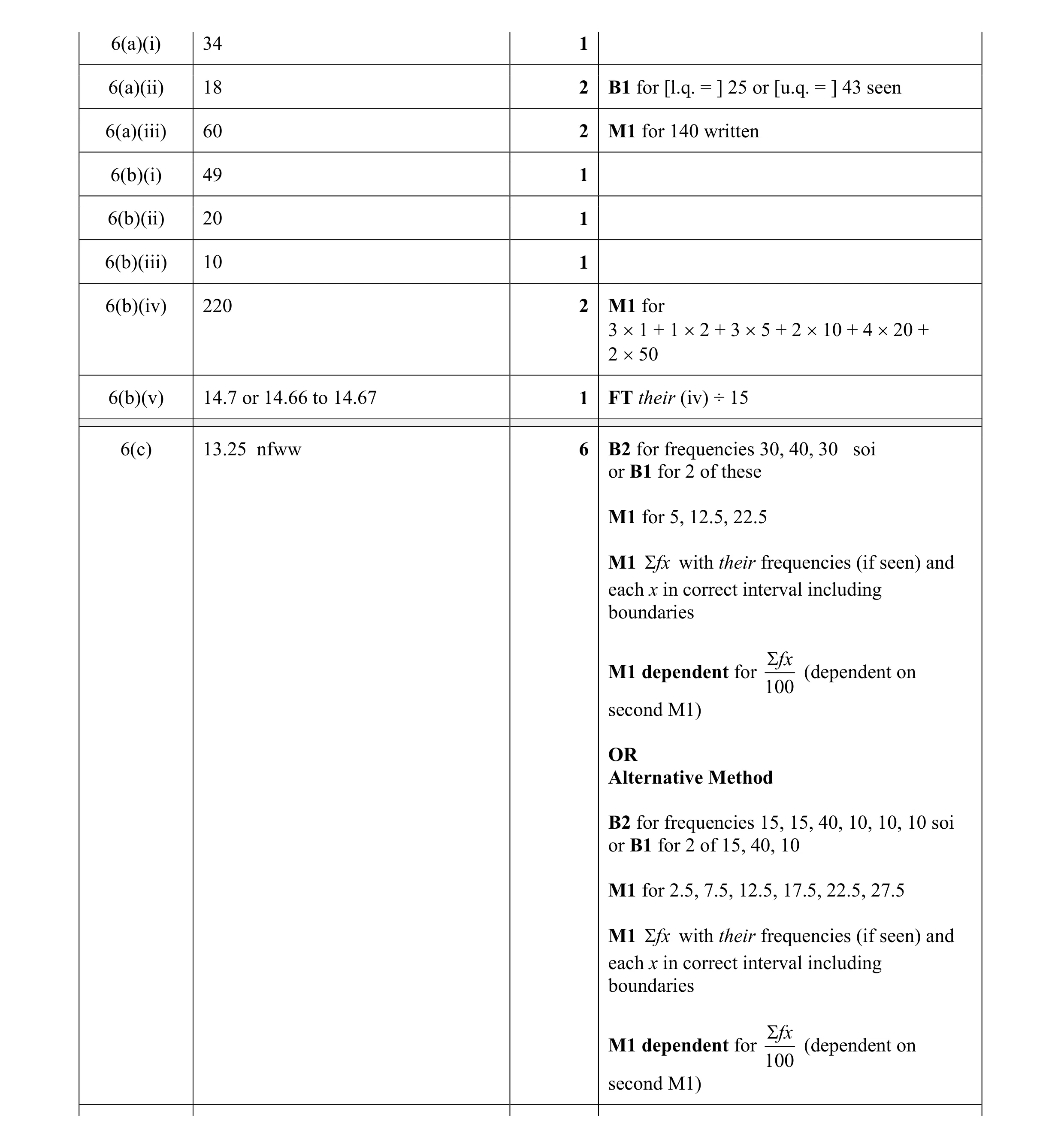 17
17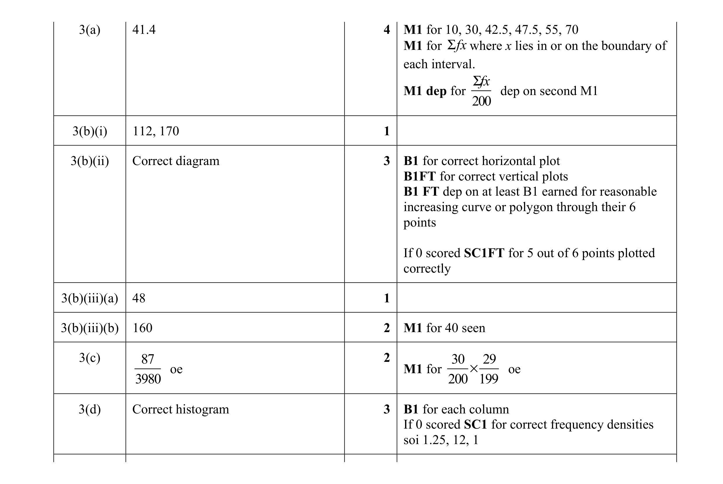 16
16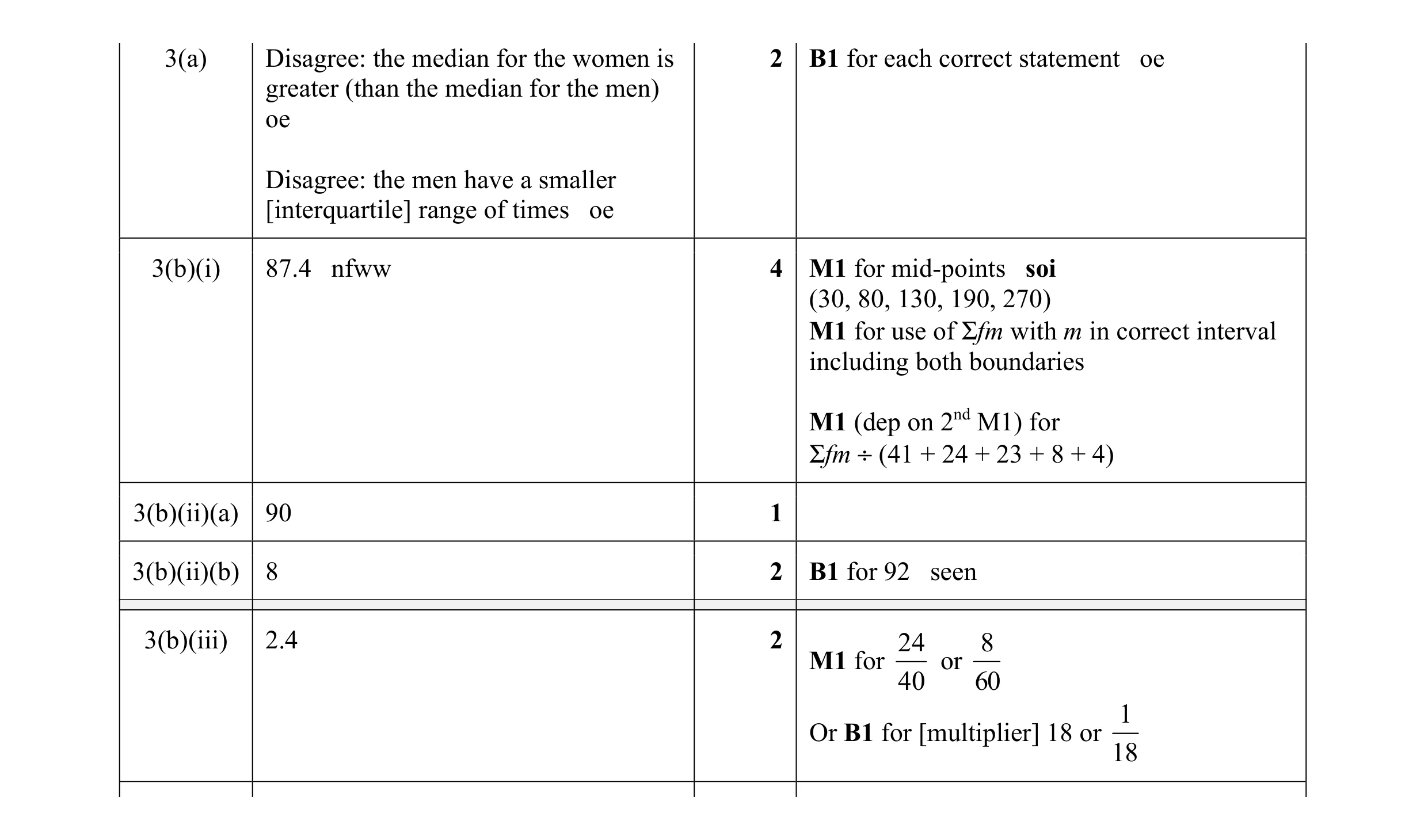 11
11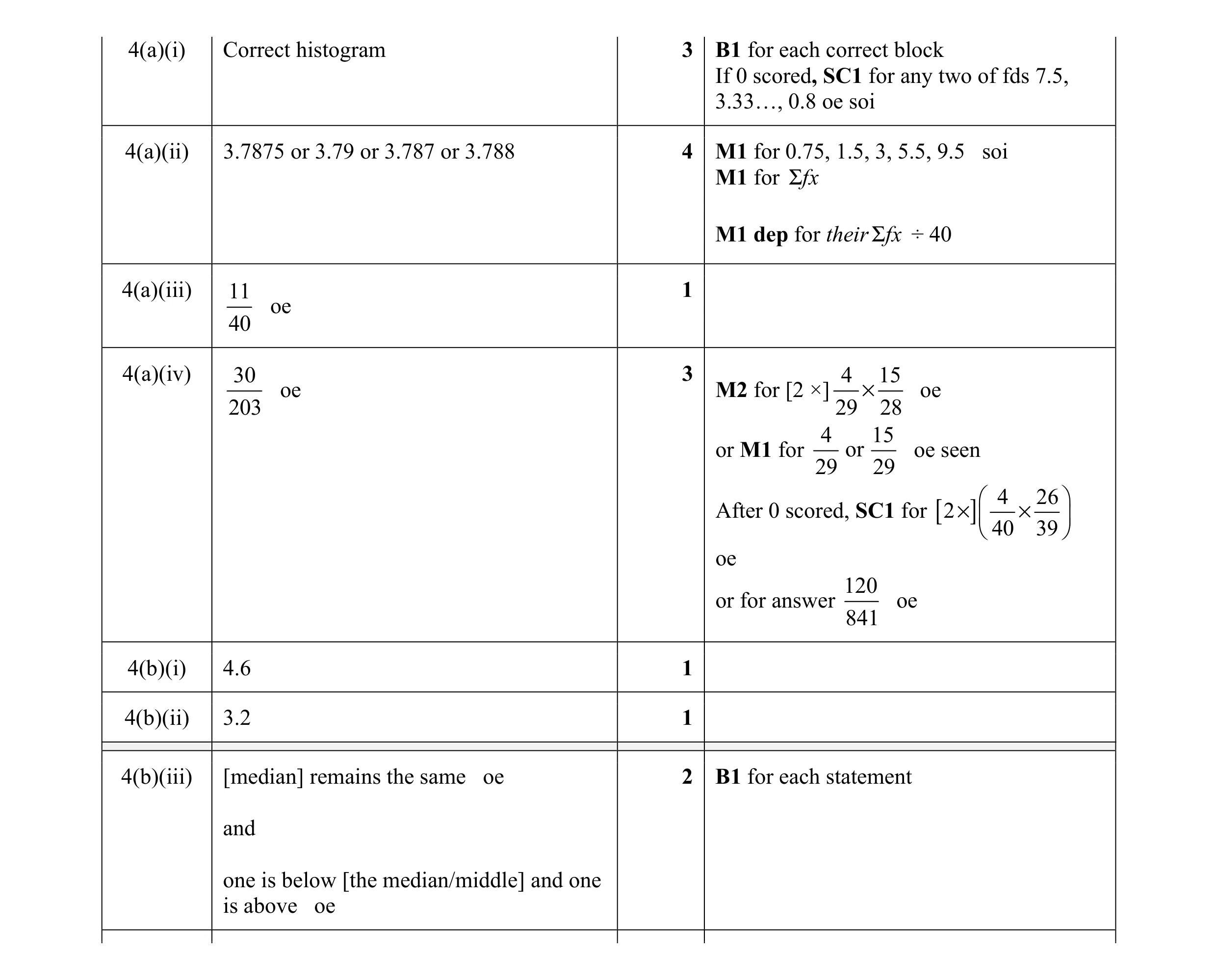 15
15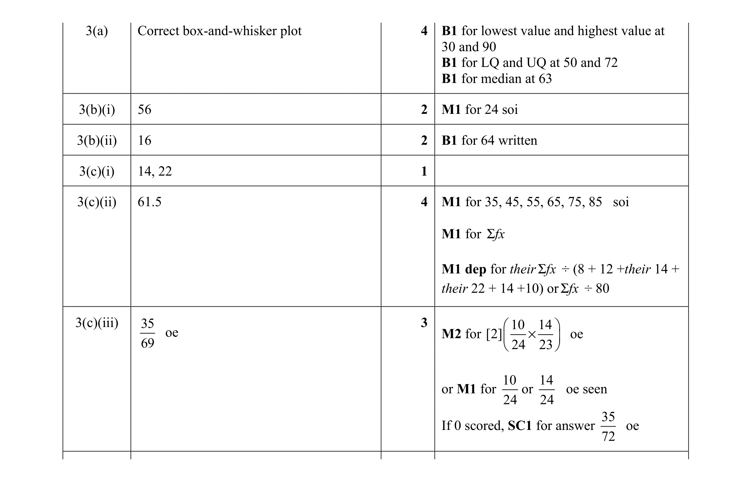 16
16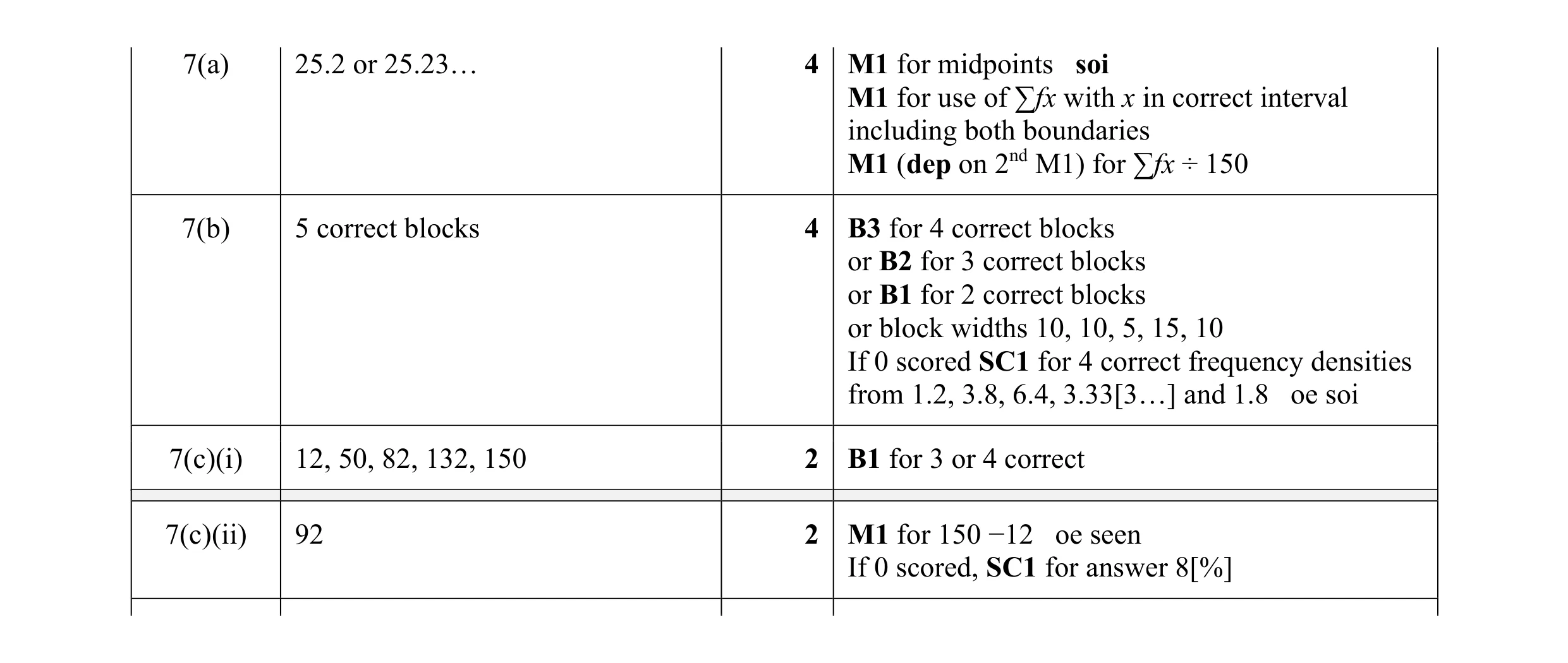 12
12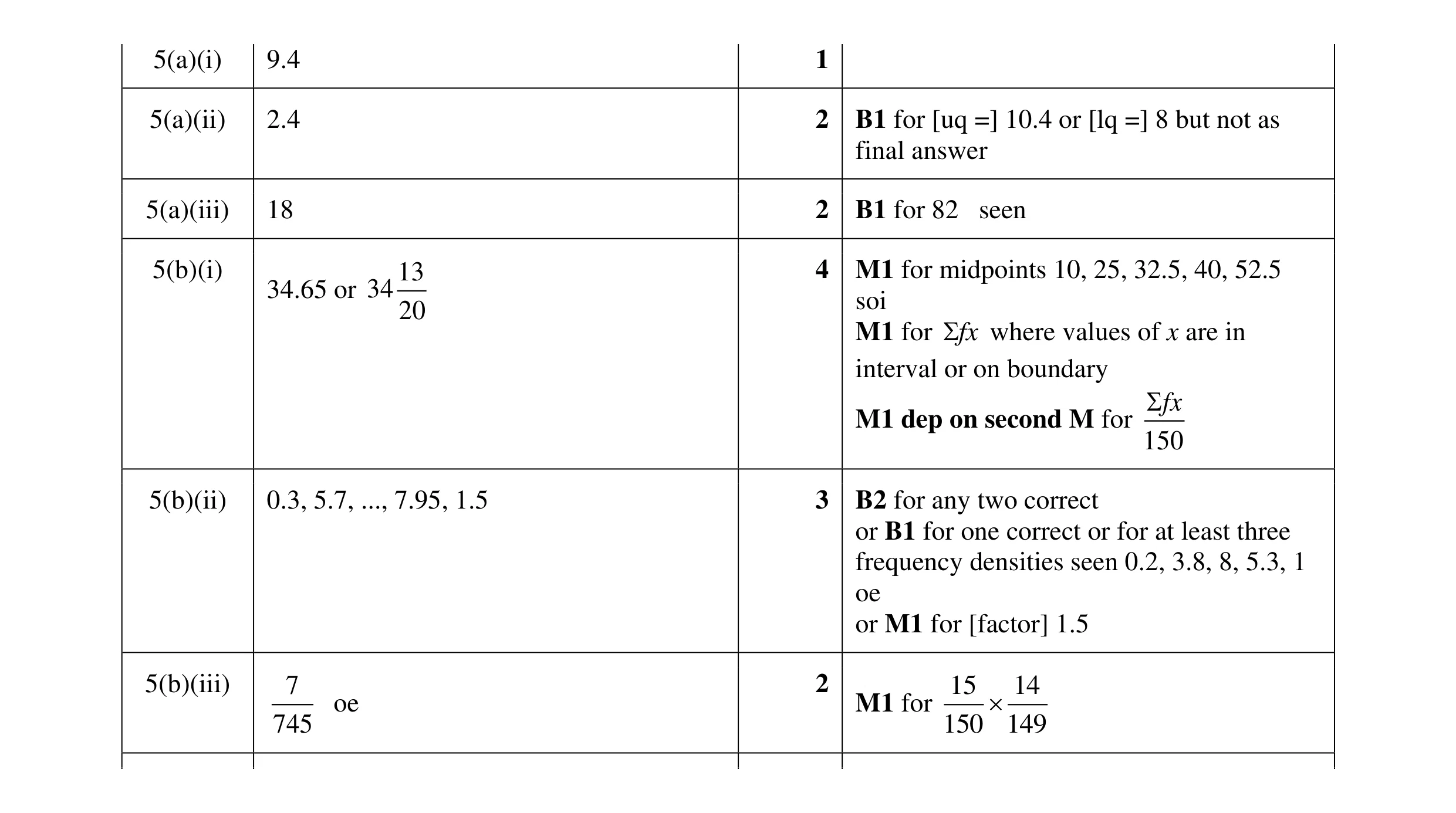 14
14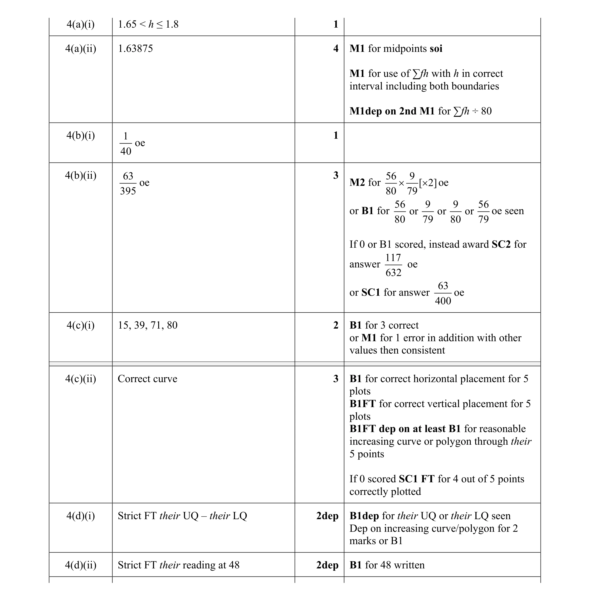 18
18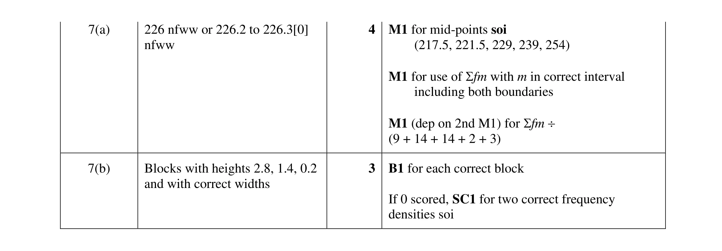 7
7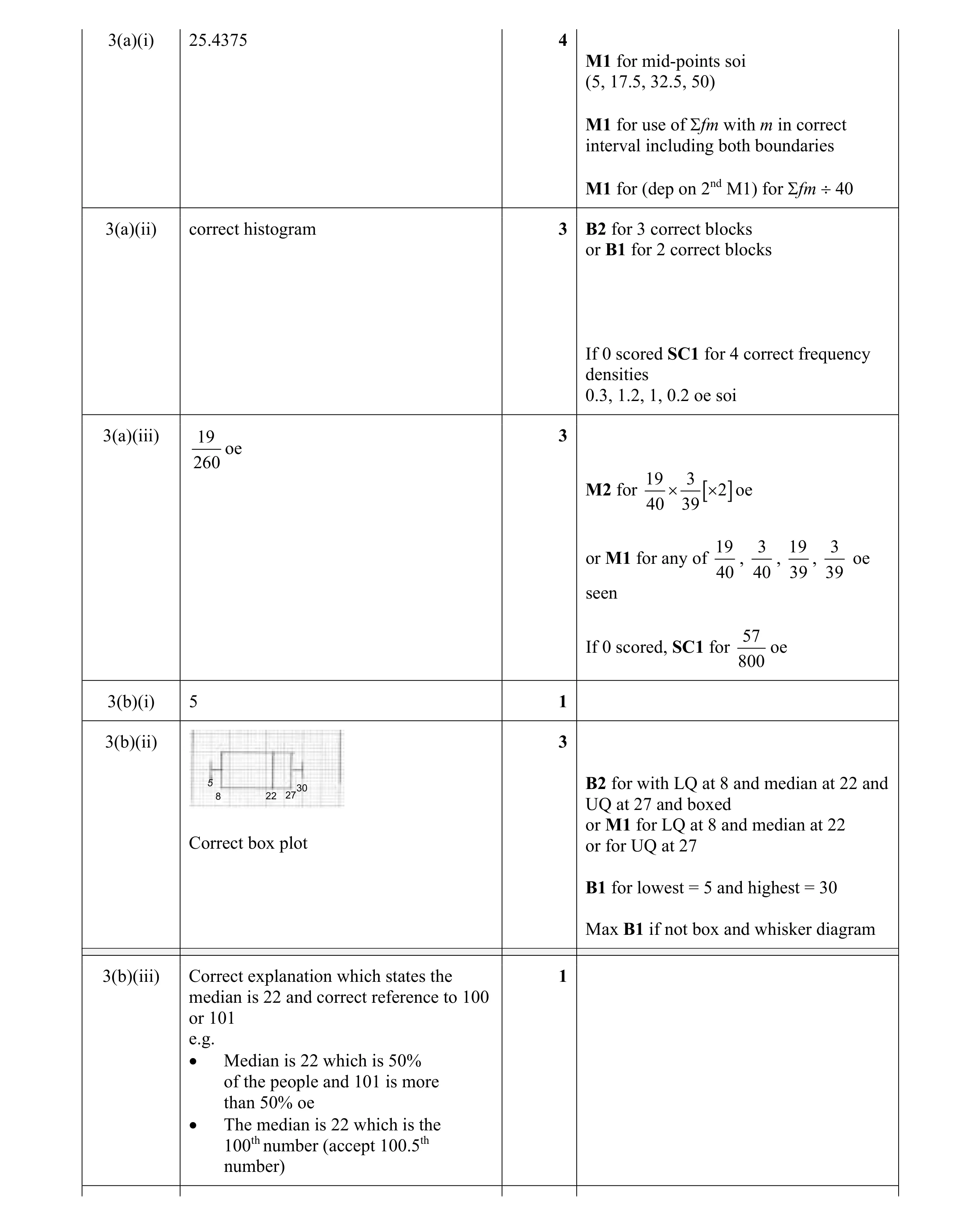 15
15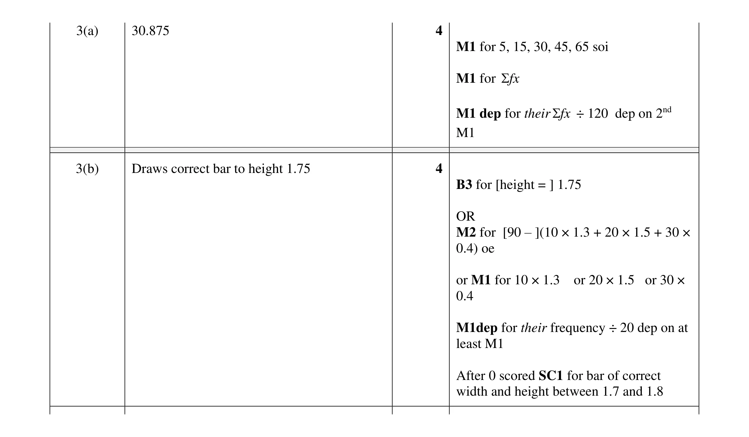 8
8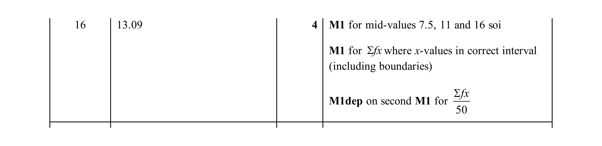 4
4