Cambridge IGCSE Geography 0460 — 2020 Oct/Nov Paper 2 · Variant 1

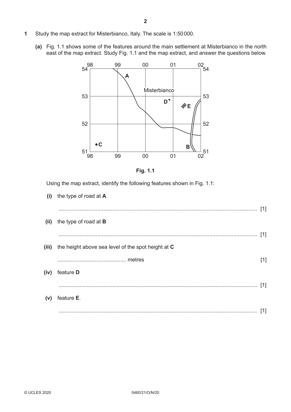
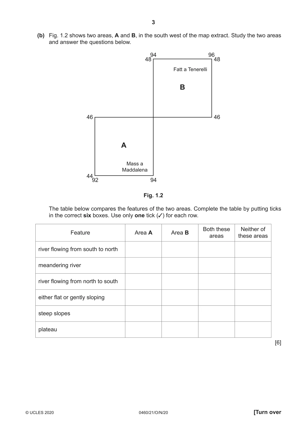
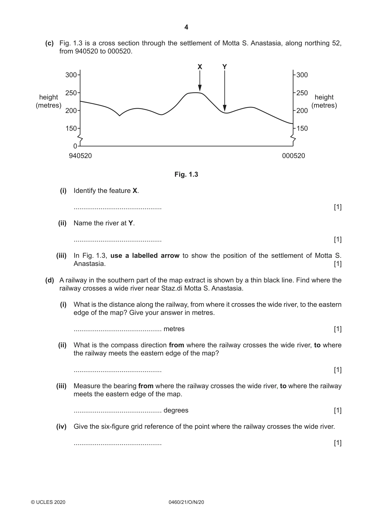
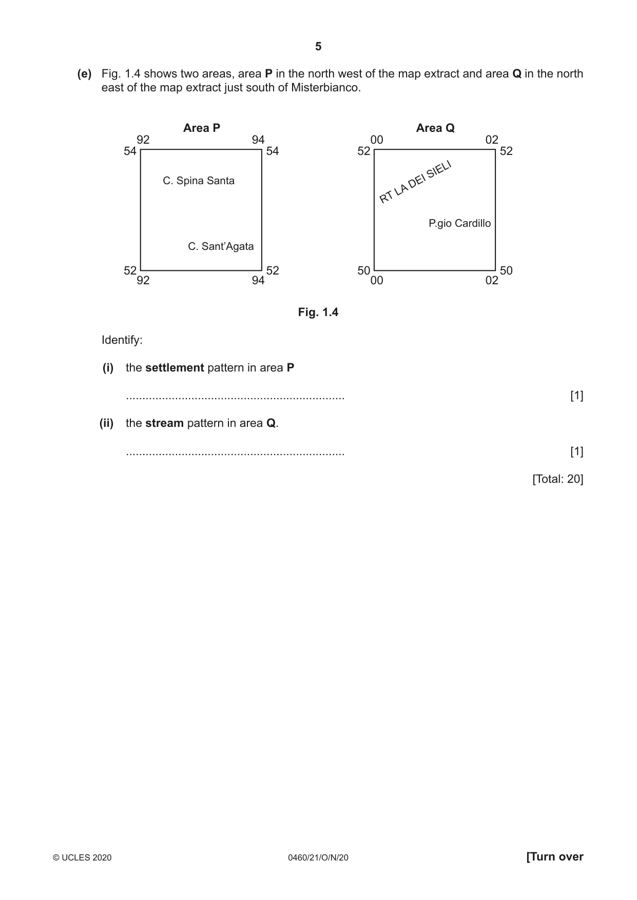
1 Study the map extract for Misterbianco, Italy. The scale is 1:50 000. (a) Fig. 1.1 shows some of the features around the main settlement at Misterbianco in the north east of the map extract. Study Fig. 1.1 and the map extract, and answer the questions below. 98 99 00 01 02 54 54 A MisterbiancoMisterbianco 53 53 D E 52 52 C B 51 51 98 99 00 01 02 Fig. 1.1 Using the map extract, identify the following features shown in Fig. 1.1: (i) the type of road at A ..................................................................................................................................... [1] (ii) the type of road at B ..................................................................................................................................... [1] (iii) the height above sea level of the spot height at C .............................................. metres [1] (iv) feature D ..................................................................................................................................... [1] (v) feature E. ..................................................................................................................................... [1] (b) Fig. 1.2 shows two areas, A and B, in the south west of the map extract. Study the two areas and answer the questions below. 4894 9648 Fatt a Tenerelli B 46 46 A Mass a Maddalena 44 92 94 Fig. 1.2 The table below compares the features of the two areas. Complete the table by putting ticks in the correct six boxes. Use only one tick (3) for each row. Both these Neither of Feature Area A Area B areas these areas river flowing from south to north meandering river river flowing from north to south either flat or gently sloping steep slopes plateau [6] (c) Fig. 1.3 is a cross section through the settlement of Motta S. Anastasia, along northing 52, from 940520 to 000520. X Y 300 300 250 250 height height (metres) (metres) 200 200 150 150 0 940520 000520 Fig. 1.3 (i) Identify the feature X. .............................................. [1] (ii) Name the river at Y. .............................................. [1] (iii) In Fig. 1.3, use a labelled arrow to show the position of the settlement of Motta S. Anastasia. [1] (d) A railway in the southern part of the map extract is shown by a thin black line. Find where the railway crosses a wide river near Staz.di Motta S. Anastasia. (i) What is the distance along the railway, from where it crosses the wide river, to the eastern edge of the map? Give your answer in metres. .............................................. metres [1] (ii) What is the compass direction from where the railway crosses the wide river, to where the railway meets the eastern edge of the map? .............................................. [1] (iii) Measure the bearing from where the railway crosses the wide river, to where the railway meets the eastern edge of the map. .............................................. degrees [1] (iv) Give the six-figure grid reference of the point where the railway crosses the wide river. .............................................. [1] (e) Fig. 1.4 shows two areas, area P in the north west of the map extract and area Q in the north east of the map extract just south of Misterbianco. Area P Area Q 92 94 00 02 54 54 52 52 SIELI C. Spina Santa DEI LA RT P.gio Cardillo C. Sant’Agata 52 52 50 50 92 94 00 02 Fig. 1.4 Identify: (i) the settlement pattern in area P ................................................................... [1] (ii) the stream pattern in area Q. ................................................................... [1] [Total: 20]

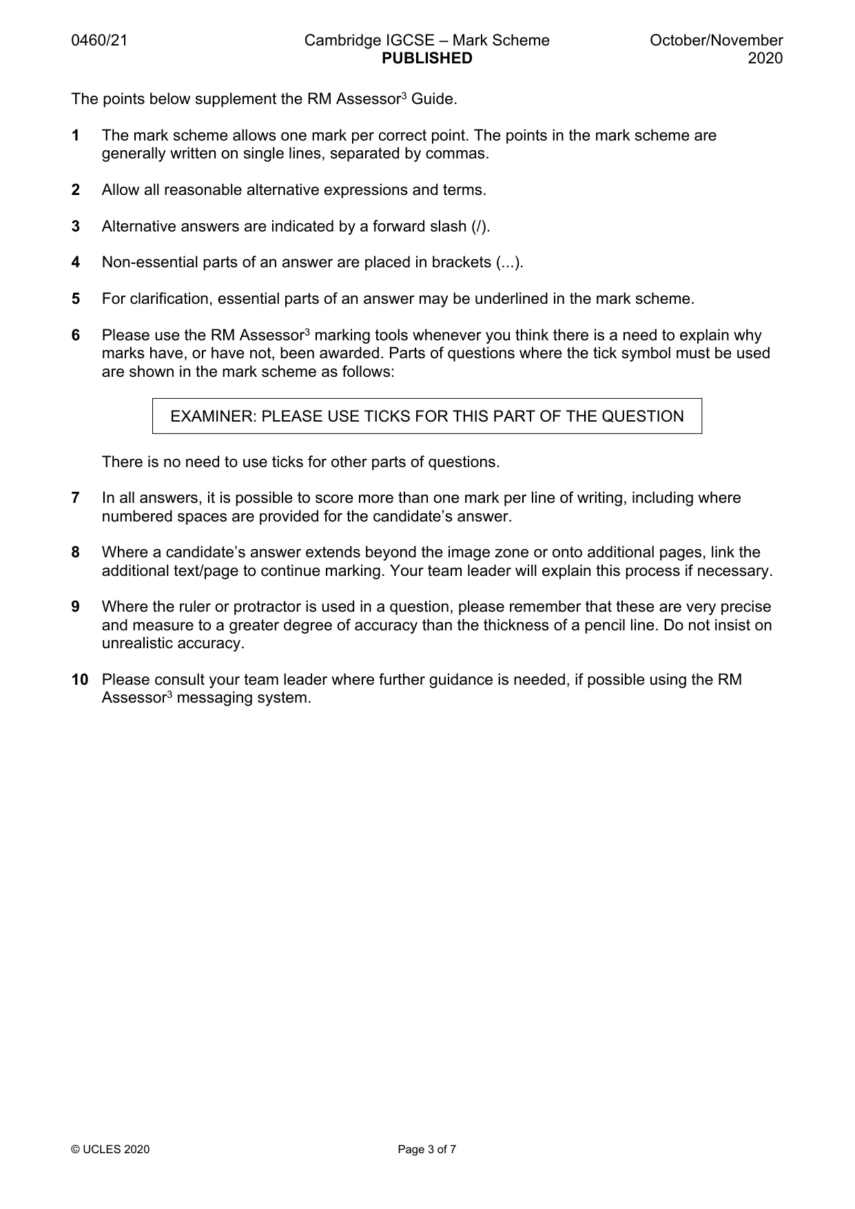
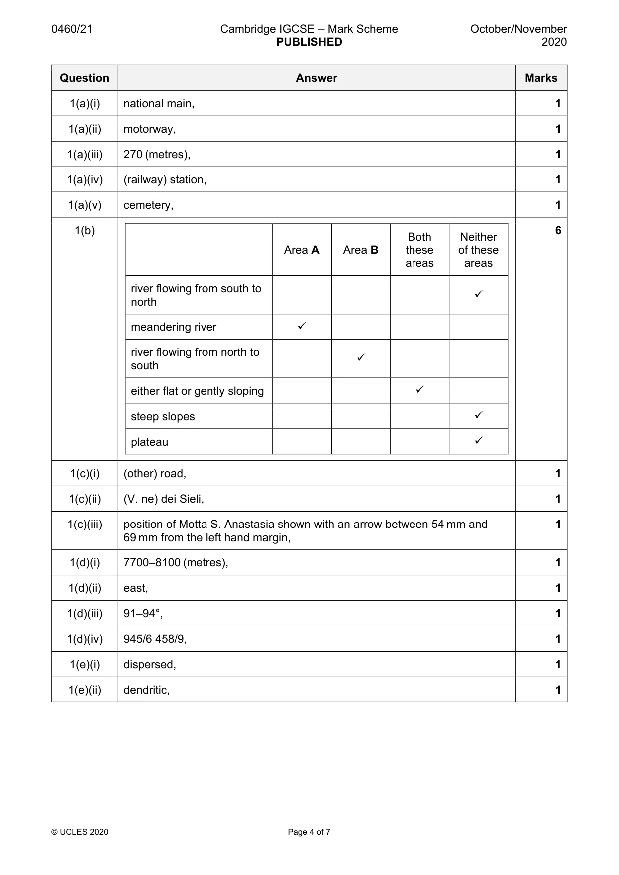
Mark scheme: Question Answer Marks 1(a)(i) national main, 1 1(a)(ii) motorway, 1 1(a)(iii) 270 (metres), 1 1(a)(iv) (railway) station, 1 1(a)(v) cemetery, 1 1(b) 6 Both Neither Area A Area B these of these areas areas river flowing from south to  north meandering river  river flowing from north to  south either flat or gently sloping  steep slopes  plateau  1(c)(i) (other) road, 1 1(c)(ii) (V. ne) dei Sieli, 1 1(c)(iii) position of Motta S. Anastasia shown with an arrow between 54 mm and 1 69 mm from the left hand margin, 1(d)(i) 7700–8100 (metres), 1 1(d)(ii) east, 1 1(d)(iii) 91–94°, 1 1(d)(iv) 945/6 458/9, 1 1(e)(i) dispersed, 1 1(e)(ii) dendritic, 1

More questions on Rivers

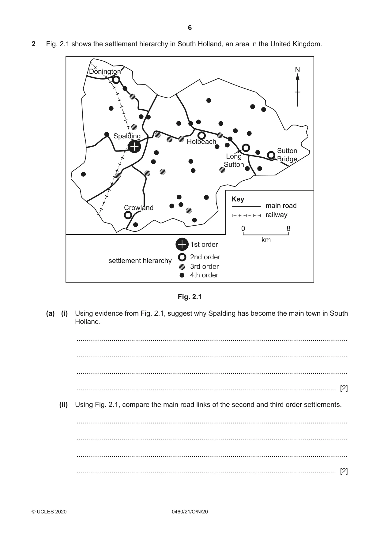
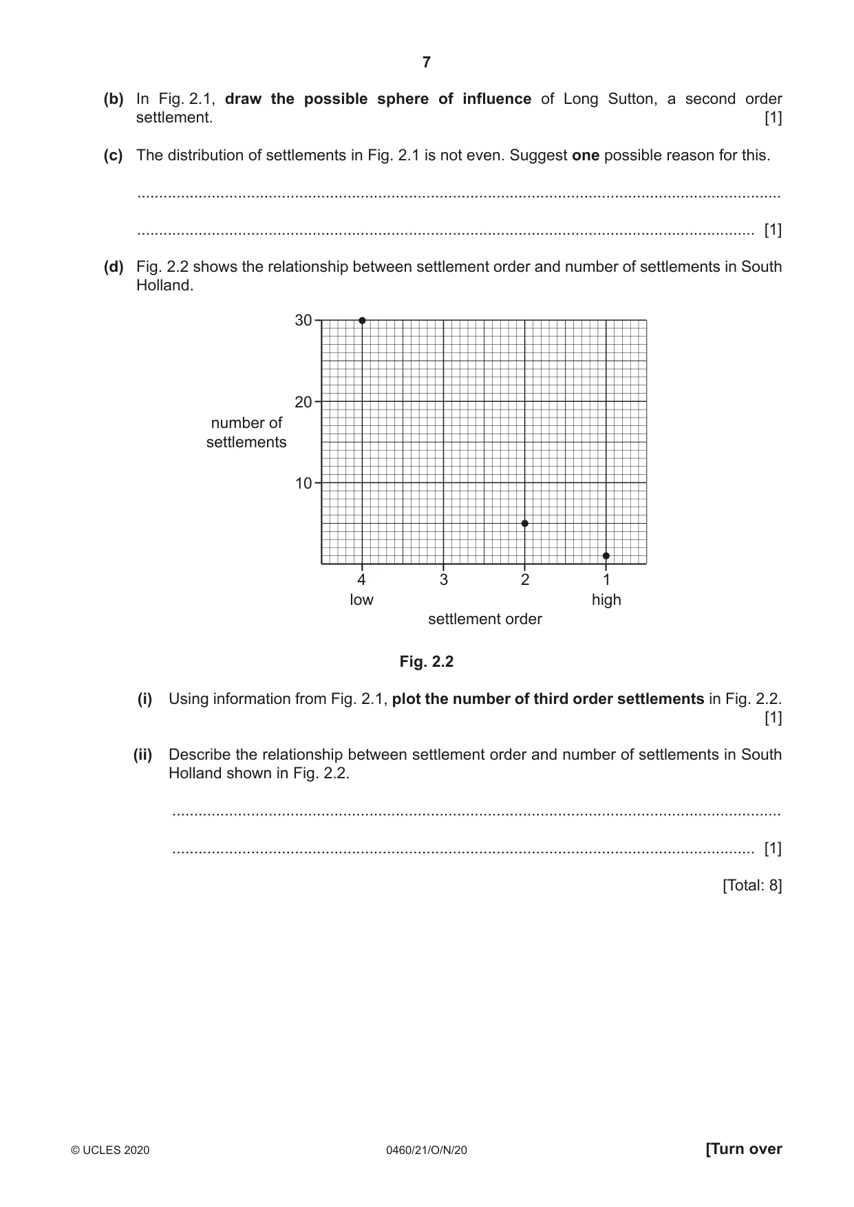
2 Fig. 2.1 shows the settlement hierarchy in South Holland, an area in the United Kingdom. N DoningtonDonington SpaldingSpalding Holbeach SuttonSutton Long BridgeBridge Sutton Key main road CrowlandCrowland railway 0 8 km 1st order 2nd order settlement hierarchy 3rd order 4th order Fig. 2.1 (a) (i) Using evidence from Fig. 2.1, suggest why Spalding has become the main town in South Holland. ........................................................................................................................................... ........................................................................................................................................... ........................................................................................................................................... ..................................................................................................................................... [2] (ii) Using Fig. 2.1, compare the main road links of the second and third order settlements. ........................................................................................................................................... ........................................................................................................................................... ........................................................................................................................................... ..................................................................................................................................... [2] (b) In Fig. 2.1, draw the possible sphere of influence of Long Sutton, a second order settlement. [1] (c) The distribution of settlements in Fig. 2.1 is not even. Suggest one possible reason for this. ................................................................................................................................................... ............................................................................................................................................. [1] (d) Fig. 2.2 shows the relationship between settlement order and number of settlements in South Holland. 30 20 number of settlements 10 4 3 2 1 low high settlement order Fig. 2.2 (i) Using information from Fig. 2.1, plot the number of third order settlements in Fig. 2.2. [1] (ii) Describe the relationship between settlement order and number of settlements in South Holland shown in Fig. 2.2. ........................................................................................................................................... ..................................................................................................................................... [1] [Total: 8]

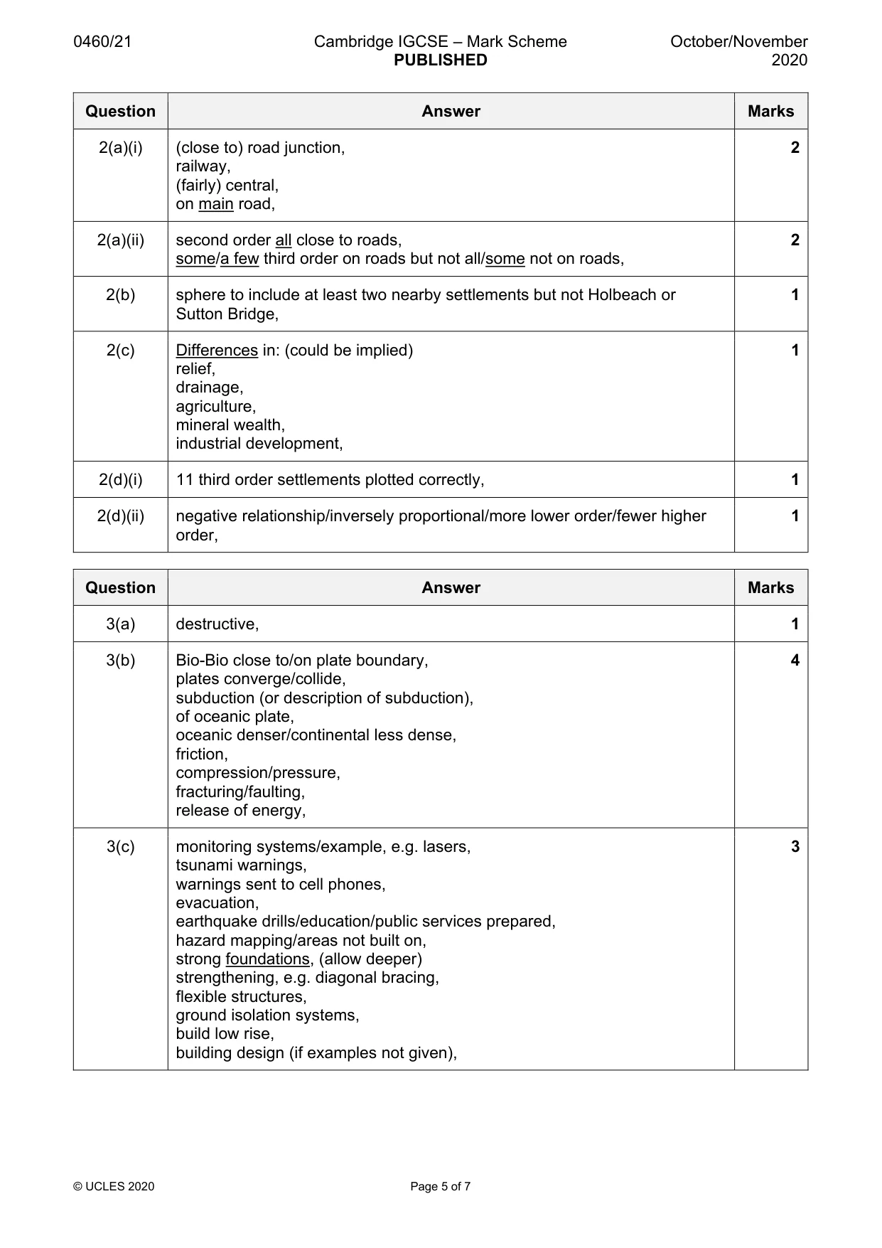
Mark scheme: 2(a)(i) (close to) road junction, 2 railway, (fairly) central, on main road, 2(a)(ii) second order all close to roads, 2 some/a few third order on roads but not all/some not on roads, 2(b) sphere to include at least two nearby settlements but not Holbeach or 1 Sutton Bridge, 2(c) Differences in: (could be implied) 1 relief, drainage, agriculture, mineral wealth, industrial development, 2(d)(i) 11 third order settlements plotted correctly, 1 2(d)(ii) negative relationship/inversely proportional/more lower order/fewer higher 1 order,

More questions on Settlements (rural and urban) and service provision

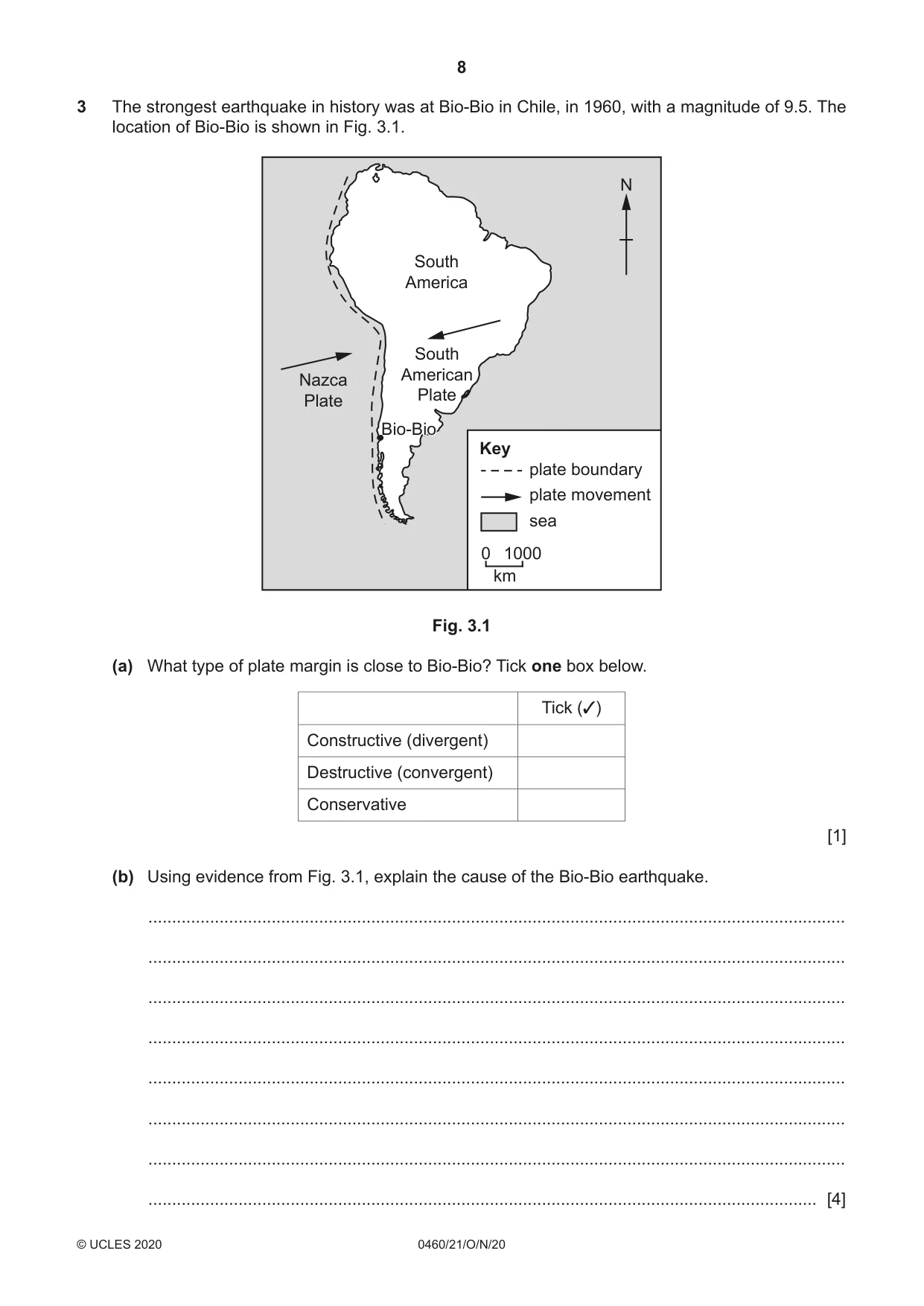
3 The strongest earthquake in history was at Bio-Bio in Chile, in 1960, with a magnitude of 9.5. The location of Bio-Bio is shown in Fig. 3.1. N South America South American Nazca Plate Plate Bio-BioBio-Bio Key plate boundary plate movement sea 0 1000 km Fig. 3.1 (a) What type of plate margin is close to Bio-Bio? Tick one box below. Tick (3) Constructive (divergent) Destructive (convergent) Conservative [1] (b) Using evidence from Fig. 3.1, explain the cause of the Bio-Bio earthquake. ................................................................................................................................................... ................................................................................................................................................... ................................................................................................................................................... ................................................................................................................................................... ................................................................................................................................................... ................................................................................................................................................... ................................................................................................................................................... ............................................................................................................................................. [4] (c) Explain what can be done to reduce the impacts of earthquakes. ................................................................................................................................................... ................................................................................................................................................... ................................................................................................................................................... ................................................................................................................................................... ................................................................................................................................................... ................................................................................................................................................... ............................................................................................................................................. [3] [Total: 8]

Mark scheme: 3(a) destructive, 1 3(b) Bio-Bio close to/on plate boundary, 4 plates converge/collide, subduction (or description of subduction), of oceanic plate, oceanic denser/continental less dense, friction, compression/pressure, fracturing/faulting, release of energy, 3(c) monitoring systems/example, e.g. lasers, 3 tsunami warnings, warnings sent to cell phones, evacuation, earthquake drills/education/public services prepared, hazard mapping/areas not built on, strong foundations, (allow deeper) strengthening, e.g. diagonal bracing, flexible structures, ground isolation systems, build low rise, building design (if examples not given),

More questions on Earthquakes and volcanoes

4 Figs. 4.1 and 4.2 (Insert) show part of a desert in southern Africa. (a) Describe the vegetation shown in Figs. 4.1 and 4.2. ................................................................................................................................................... ................................................................................................................................................... ................................................................................................................................................... ................................................................................................................................................... ................................................................................................................................................... ................................................................................................................................................... ................................................................................................................................................... ................................................................................................................................................... ................................................................................................................................................... ................................................................................................................................................... ............................................................................................................................................. [5] (b) Fig. 4.2 also shows a waste heap produced by the mining of copper ore. Suggest how this may pose a threat to the natural environment. ................................................................................................................................................... ................................................................................................................................................... ................................................................................................................................................... ................................................................................................................................................... ................................................................................................................................................... ................................................................................................................................................... ............................................................................................................................................. [3] [Total: 8]

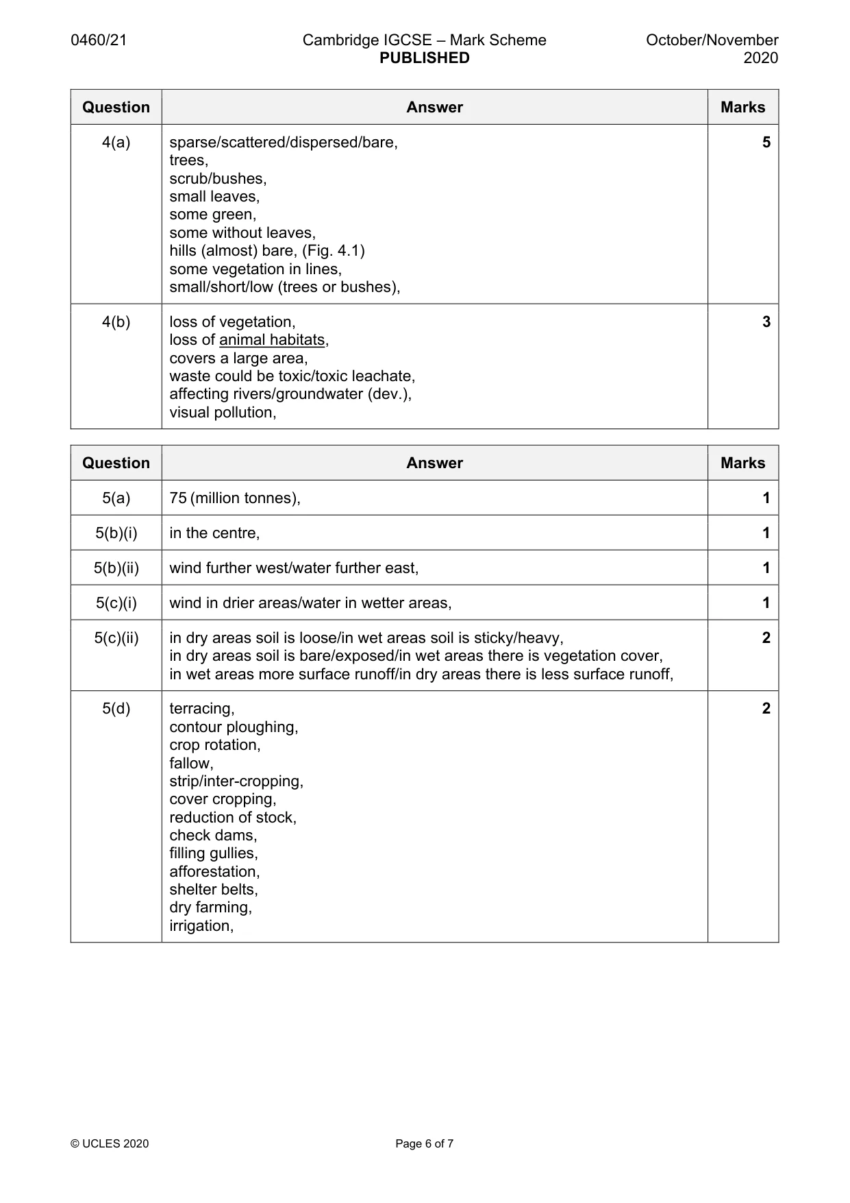
Mark scheme: 4(a) sparse/scattered/dispersed/bare, 5 trees, scrub/bushes, small leaves, some green, some without leaves, hills (almost) bare, (Fig. 4.1) some vegetation in lines, small/short/low (trees or bushes), 4(b) loss of vegetation, 3 loss of animal habitats, covers a large area, waste could be toxic/toxic leachate, affecting rivers/groundwater (dev.), visual pollution,

More questions on Climate and natural vegetation

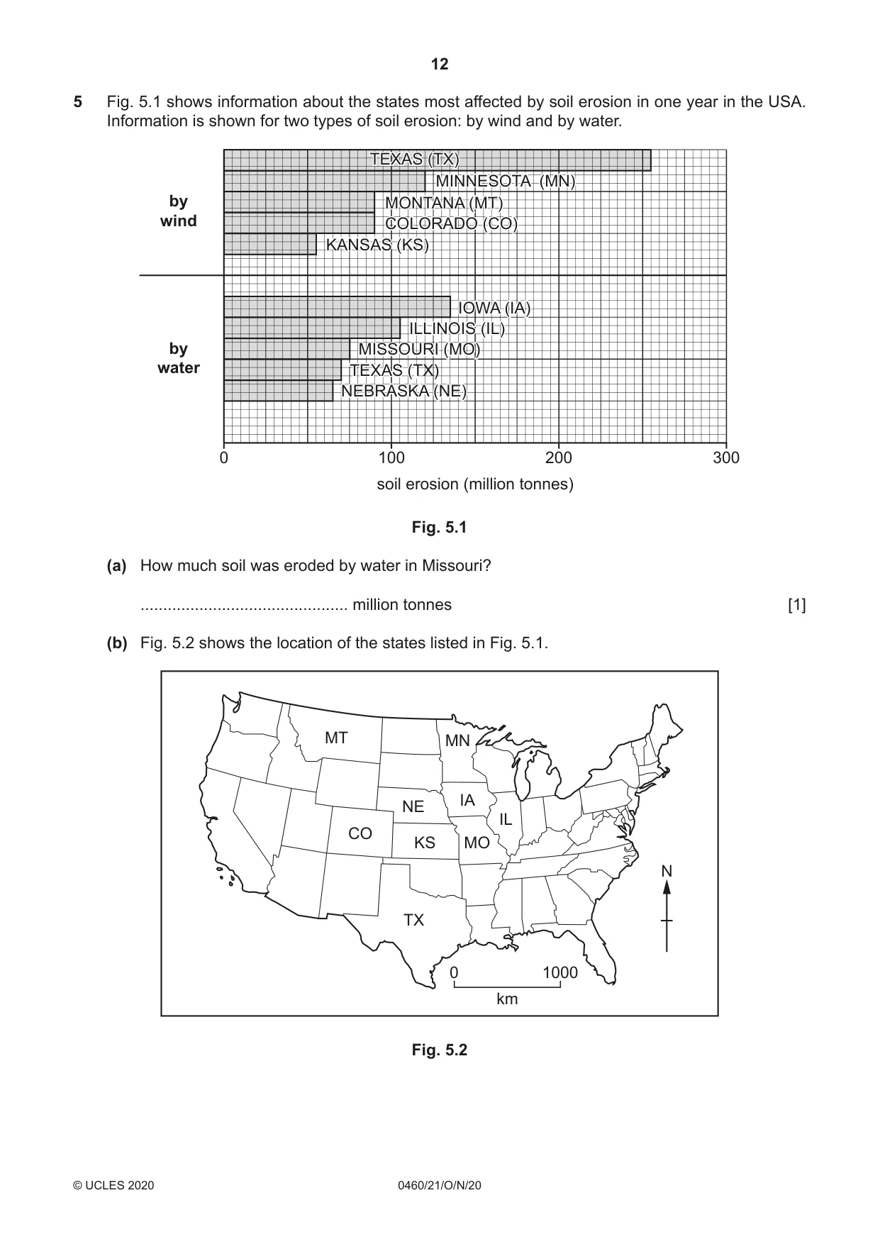
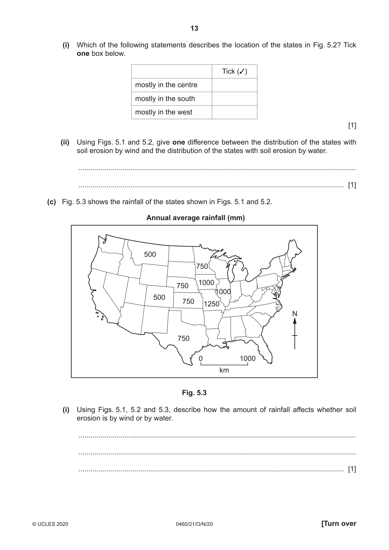
5 Fig. 5.1 shows information about the states most affected by soil erosion in one year in the USA. Information is shown for two types of soil erosion: by wind and by water. TEXASTEXAS (TX)(TX) MINNESOTAMINNESOTA (MN)(MN) by MONTANAMONTANA (MT)(MT) wind COLORADOCOLORADO (CO)(CO) KANSASKANSAS (KS)(KS) IOWAIOWA (IA)(IA) ILLINOISILLINOIS (IL)(IL) by MISSOURIMISSOURI (MO)(MO) water TEXASTEXAS ()(TX) NEBRASKANEBRASKA (NE)(NE) 0 100 200 300 soil erosion (million tonnes) Fig. 5.1 (a) How much soil was eroded by water in Missouri? .............................................. million tonnes [1] (b) Fig. 5.2 shows the location of the states listed in Fig. 5.1. MT MN IA NE IL CO KS MO N TX 0 1000 km Fig. 5.2 (i) Which of the following statements describes the location of the states in Fig. 5.2? Tick one box below. Tick (3) mostly in the centre mostly in the south mostly in the west [1] (ii) Using Figs. 5.1 and 5.2, give one difference between the distribution of the states with soil erosion by wind and the distribution of the states with soil erosion by water. ........................................................................................................................................... ..................................................................................................................................... [1] (c) Fig. 5.3 shows the rainfall of the states shown in Figs. 5.1 and 5.2. Annual average rainfall (mm) 500 750 1000 750 1000 50025 750 1250 N 500750– 750 0 1000 km Fig. 5.3 (i) Using Figs. 5.1, 5.2 and 5.3, describe how the amount of rainfall affects whether soil erosion is by wind or by water. ........................................................................................................................................... ........................................................................................................................................... ..................................................................................................................................... [1] (ii) Explain why the amount of rainfall affects whether soil erosion is by wind or by water. ........................................................................................................................................... ........................................................................................................................................... ........................................................................................................................................... ........................................................................................................................................... ..................................................................................................................................... [2] (d) Give two ways of preventing or reducing soil erosion. 1 ................................................................................................................................................ ................................................................................................................................................... 2 ................................................................................................................................................ ............................................................................................................................................. [2] [Total: 8] TURN PAGE FOR QUESTION 6

Mark scheme: 5(a) 75 (million tonnes), 1 5(b)(i) in the centre, 1 5(b)(ii) wind further west/water further east, 1 5(c)(i) wind in drier areas/water in wetter areas, 1 5(c)(ii) in dry areas soil is loose/in wet areas soil is sticky/heavy, 2 in dry areas soil is bare/exposed/in wet areas there is vegetation cover, in wet areas more surface runoff/in dry areas there is less surface runoff, 5(d) terracing, 2 contour ploughing, crop rotation, fallow, strip/inter-cropping, cover cropping, reduction of stock, check dams, filling gullies, afforestation, shelter belts, dry farming, irrigation,

More questions on Food production

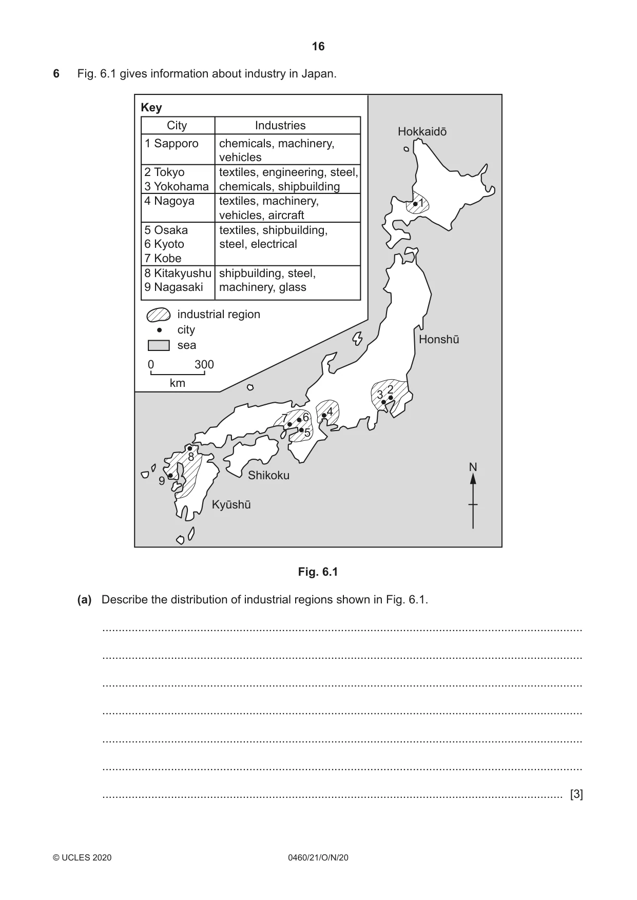
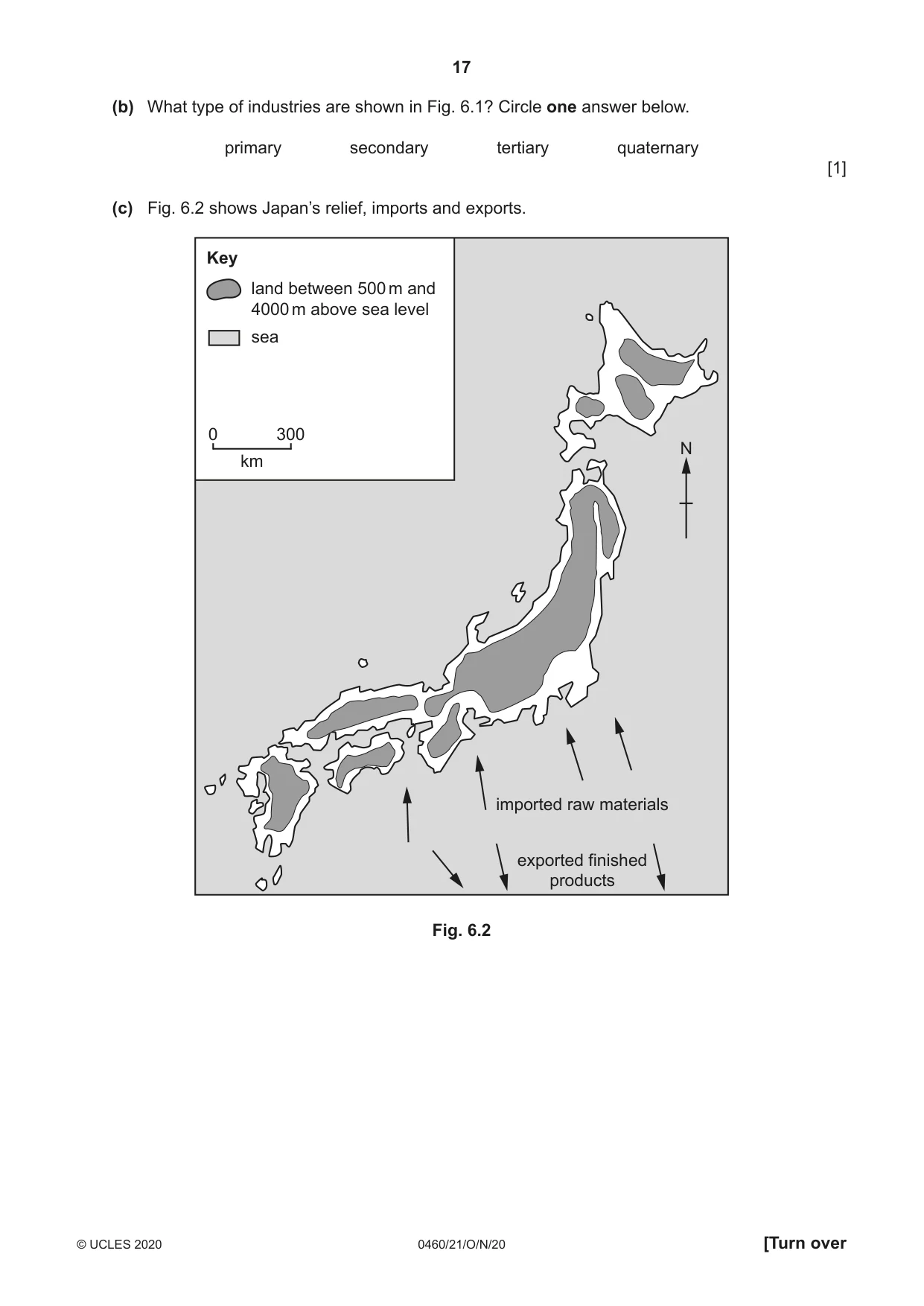
6 Fig. 6.1 gives information about industry in Japan. Key City Industries Hokkaidō 1 Sapporo chemicals, machinery, vehicles 2 Tokyo textiles, engineering, steel, 3 Yokohama chemicals, shipbuilding 4 Nagoya textiles, machinery, 11 vehicles, aircraft 5 Osaka textiles, shipbuilding, 6 Kyoto steel, electrical 7 Kobe 8 Kitakyushu shipbuilding, steel, 9 Nagasaki machinery, glass industrial region city Honshū sea 0 300 km 22 33 44 7 66 55 88 N Shikoku 9 Kyūshū Fig. 6.1 (a) Describe the distribution of industrial regions shown in Fig. 6.1. ................................................................................................................................................... ................................................................................................................................................... ................................................................................................................................................... ................................................................................................................................................... ................................................................................................................................................... ................................................................................................................................................... ............................................................................................................................................. [3] (b) What type of industries are shown in Fig. 6.1? Circle one answer below. primary secondary tertiary quaternary [1] (c) Fig. 6.2 shows Japan’s relief, imports and exports. Key land between 500 m and 4000 m above sea level sea 0 300 N km imported raw materials exported finished products Fig. 6.2 Using evidence from Figs. 6.1 and 6.2 only, explain the factors which have influenced the location of industrial regions in Japan. ................................................................................................................................................... ................................................................................................................................................... ................................................................................................................................................... ................................................................................................................................................... ................................................................................................................................................... ................................................................................................................................................... ................................................................................................................................................... ................................................................................................................................................... ................................................................................................................................................... ............................................................................................................................................. [4] [Total: 8]

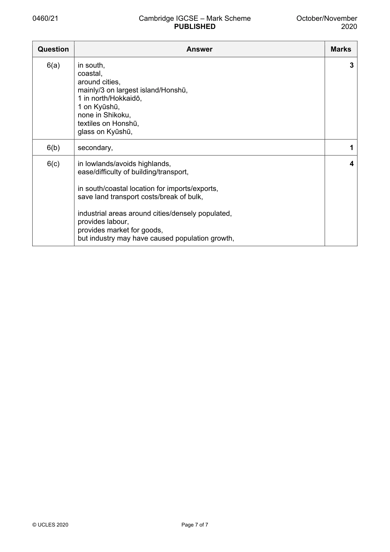
Mark scheme: 6(a) in south, 3 coastal, around cities, mainly/3 on largest island/Honshū, 1 in north/Hokkaidō, 1 on Kyūshū, none in Shikoku, textiles on Honshū, glass on Kyūshū, 6(b) secondary, 1 6(c) in lowlands/avoids highlands, 4 ease/difficulty of building/transport, in south/coastal location for imports/exports, save land transport costs/break of bulk, industrial areas around cities/densely populated, provides labour, provides market for goods, but industry may have caused population growth,

More questions on Industry