Cambridge IGCSE Geography 0460 — 2021 May/June Paper 4 · Variant 3

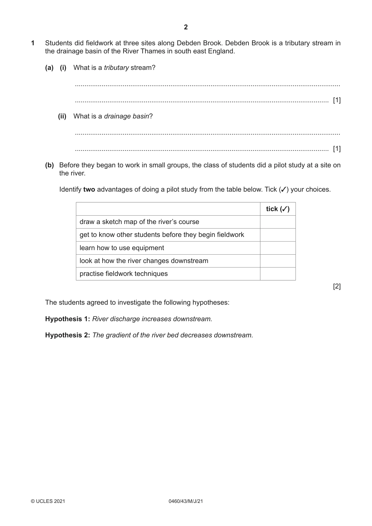
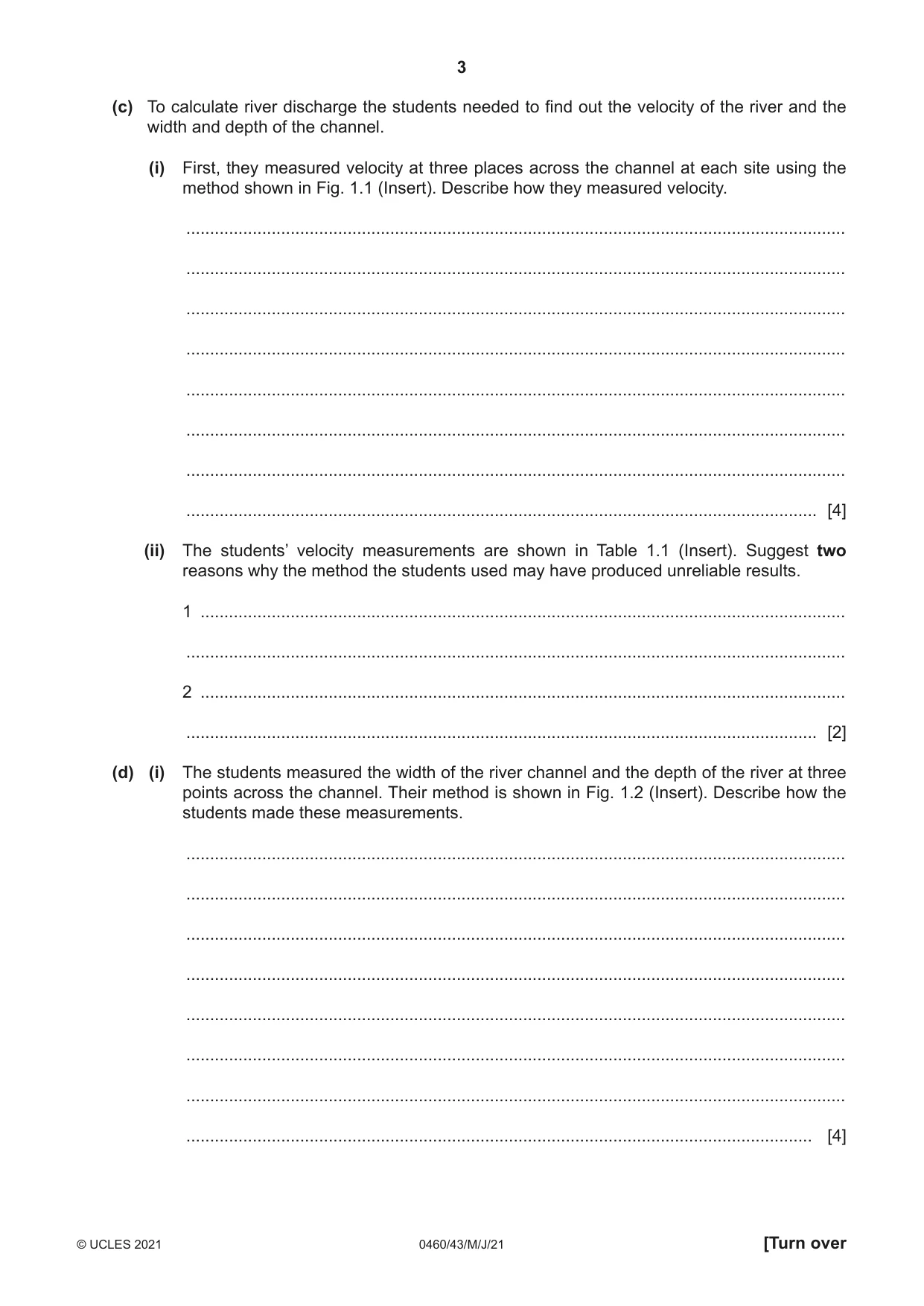
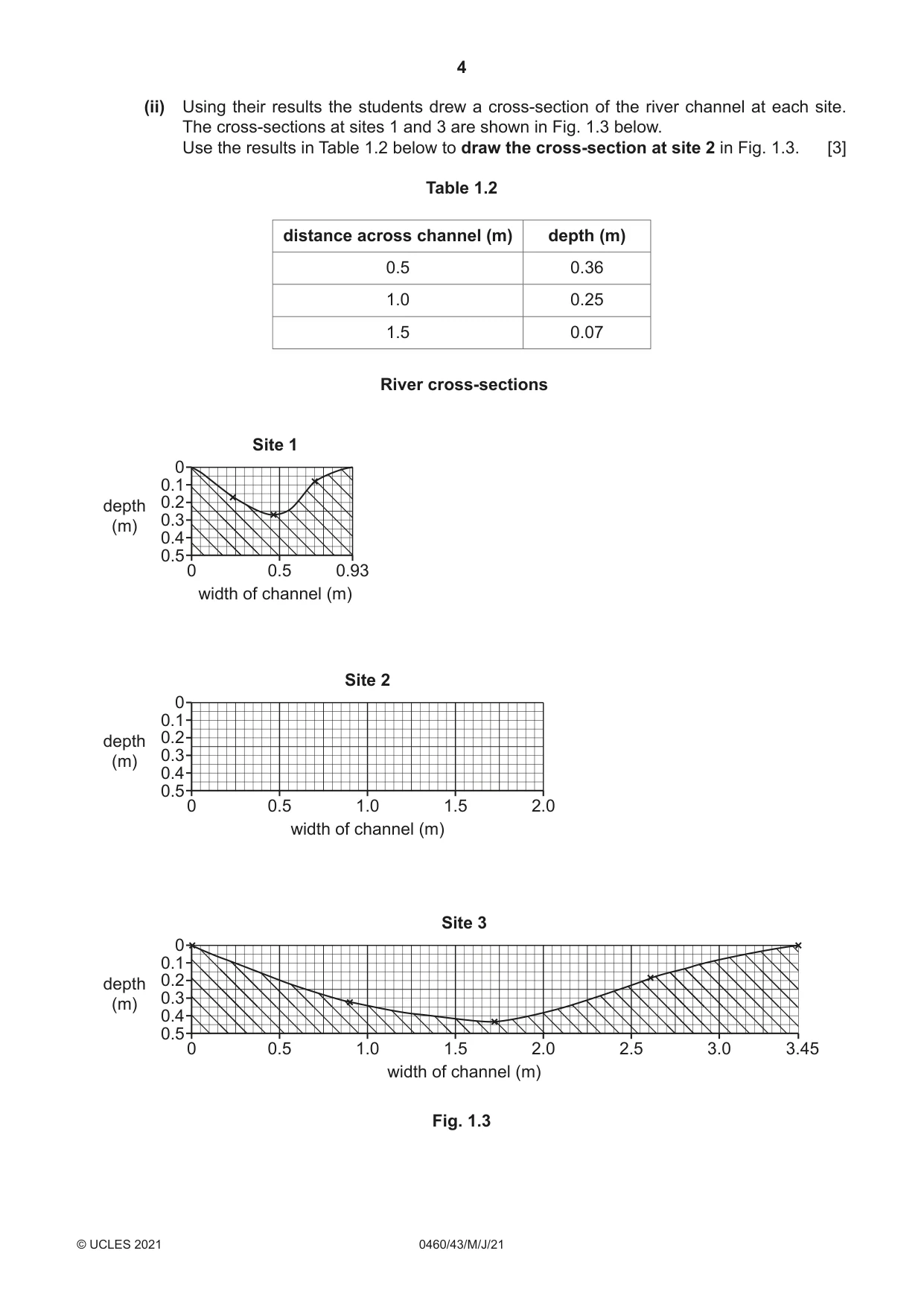
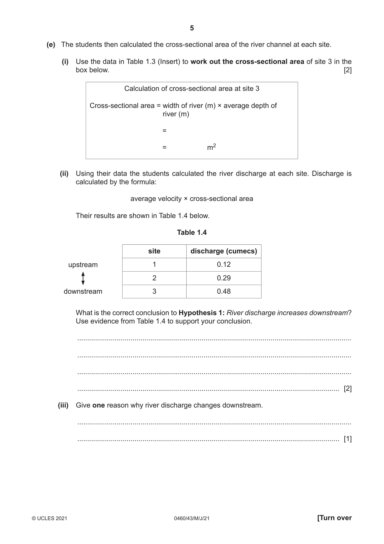
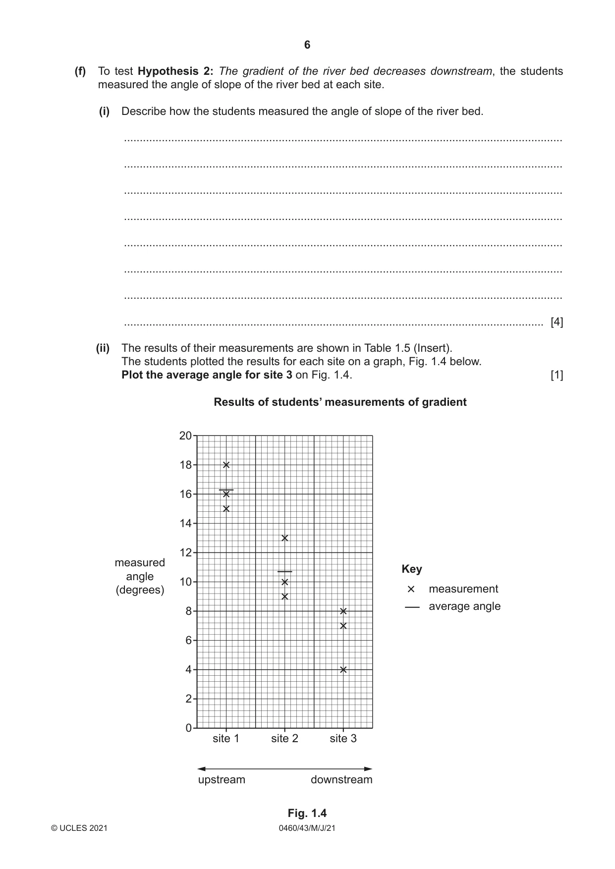
1 Students did fieldwork at three sites along Debden Brook. Debden Brook is a tributary stream in the drainage basin of the River Thames in south east England. (a) (i) What is a tributary stream? ........................................................................................................................................... ..................................................................................................................................... [1] (ii) What is a drainage basin? ........................................................................................................................................... ..................................................................................................................................... [1] (b) Before they began to work in small groups, the class of students did a pilot study at a site on the river. Identify two advantages of doing a pilot study from the table below. Tick (✓) your choices. tick (✓) draw a sketch map of the river’s course get to know other students before they begin fieldwork learn how to use equipment look at how the river changes downstream practise fieldwork techniques [2] The students agreed to investigate the following hypotheses: Hypothesis 1: River discharge increases downstream. Hypothesis 2: The gradient of the river bed decreases downstream. (c) To calculate river discharge the students needed to find out the velocity of the river and the width and depth of the channel. (i) First, they measured velocity at three places across the channel at each site using the method shown in Fig. 1.1 (Insert). Describe how they measured velocity. ........................................................................................................................................... ........................................................................................................................................... ........................................................................................................................................... ........................................................................................................................................... ........................................................................................................................................... ........................................................................................................................................... ........................................................................................................................................... ..................................................................................................................................... [4] (ii) The students’ velocity measurements are shown in Table 1.1 (Insert). Suggest two reasons why the method the students used may have produced unreliable results. 1 ........................................................................................................................................ ........................................................................................................................................... 2 ........................................................................................................................................ ..................................................................................................................................... [2] (d) (i) The students measured the width of the river channel and the depth of the river at three points across the channel. Their method is shown in Fig. 1.2 (Insert). Describe how the students made these measurements. ........................................................................................................................................... ........................................................................................................................................... ........................................................................................................................................... ........................................................................................................................................... ........................................................................................................................................... ........................................................................................................................................... ........................................................................................................................................... .................................................................................................................................... [4] (ii) Using their results the students drew a cross-section of the river channel at each site. The cross-sections at sites 1 and 3 are shown in Fig. 1.3 below. Use the results in Table 1.2 below to draw the cross-section at site 2 in Fig. 1.3. [3] Table 1.2 distance across channel (m) depth (m) 0.5 0.36 1.0 0.25 1.5 0.07 River cross-sections Site 1 0 0.1 depth 0.2 0.3 (m) 0.4 0.5 0 0.5 0.93 width of channel (m) Site 2 0 0.1 depth 0.2 0.3 (m) 0.4 0.5 0 0.5 1.0 1.5 2.0 width of channel (m) Site 3 0 0.1 depth 0.2 0.3 (m) 0.4 0.5 0 0.5 1.0 1.5 2.0 2.5 3.0 3.45 width of channel (m) Fig. 1.3 (e) The students then calculated the cross-sectional area of the river channel at each site. (i) Use the data in Table 1.3 (Insert) to work out the cross-sectional area of site 3 in the box below. [2] Calculation of cross-sectional area at site 3 Cross-sectional area = width of river (m) × average depth of river (m) = = m2 (ii) Using their data the students calculated the river discharge at each site. Discharge is calculated by the formula: average velocity × cross-sectional area Their results are shown in Table 1.4 below. Table 1.4 site discharge (cumecs) upstream 1 0.12 2 0.29 downstream 3 0.48 What is the correct conclusion to Hypothesis 1: River discharge increases downstream? Use evidence from Table 1.4 to support your conclusion. ........................................................................................................................................... ........................................................................................................................................... ........................................................................................................................................... ..................................................................................................................................... [2] (iii) Give one reason why river discharge changes downstream. ........................................................................................................................................... ..................................................................................................................................... [1] (f) To test Hypothesis 2: The gradient of the river bed decreases downstream, the students measured the angle of slope of the river bed at each site. (i) Describe how the students measured the angle of slope of the river bed. ........................................................................................................................................... ........................................................................................................................................... ........................................................................................................................................... ........................................................................................................................................... ........................................................................................................................................... ........................................................................................................................................... ........................................................................................................................................... ..................................................................................................................................... [4] (ii) The results of their measurements are shown in Table 1.5 (Insert). The students plotted the results for each site on a graph, Fig. 1.4 below. Plot the average angle for site 3 on Fig. 1.4. [1] Results of students’ measurements of gradient 20 18 16 14 12 measured Key angle 10 (degrees) measurement average angle 8 6 4 2 0 site 1 site 2 site 3 upstream downstream Fig. 1.4 (iii) Do the results shown in Fig. 1.4 and Table 1.5 (Insert) support Hypothesis 2: The gradient of the river bed decreases downstream? Use data to support your conclusion. ........................................................................................................................................... ........................................................................................................................................... ........................................................................................................................................... ........................................................................................................................................... ........................................................................................................................................... ..................................................................................................................................... [3] [Total: 30]

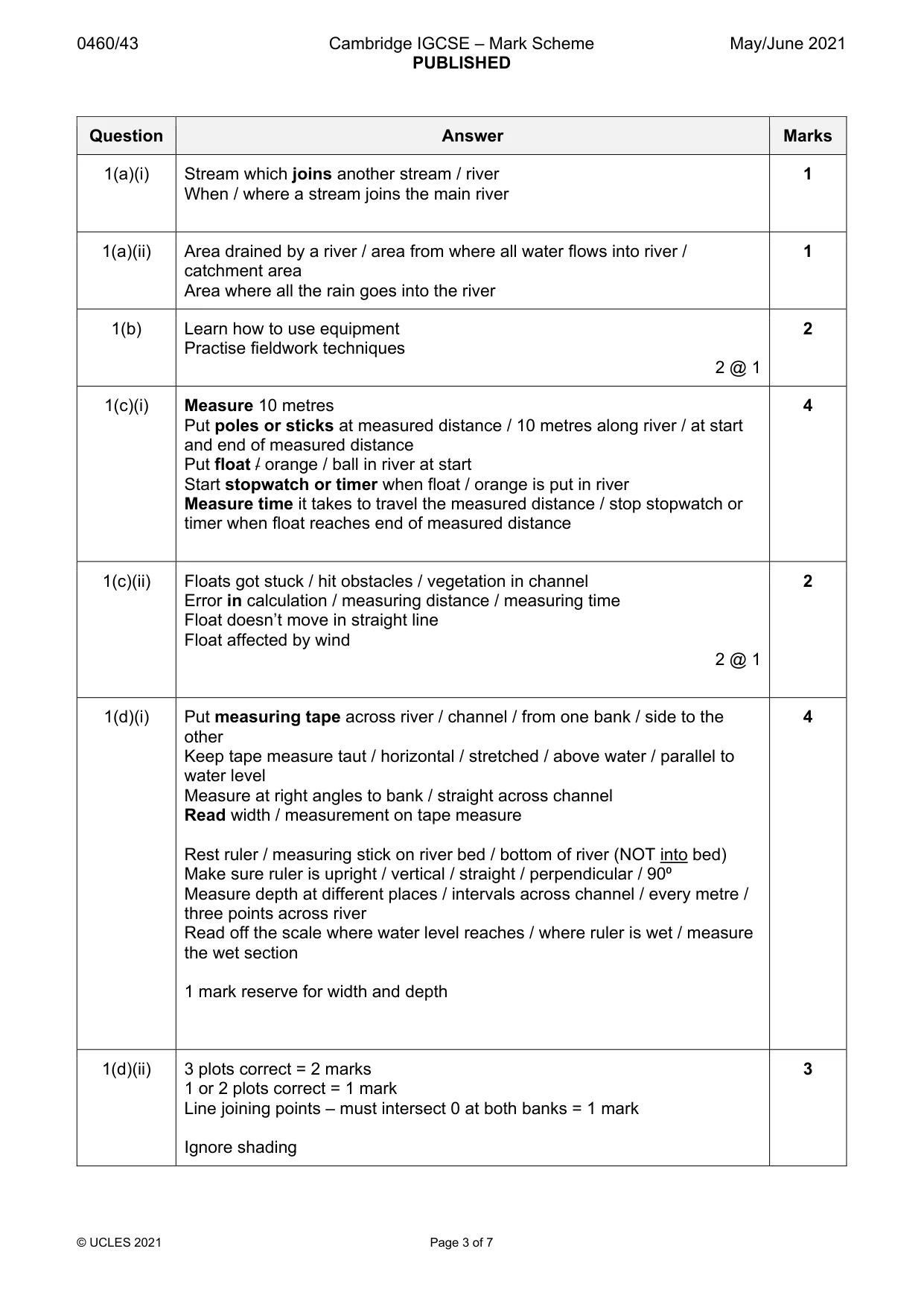
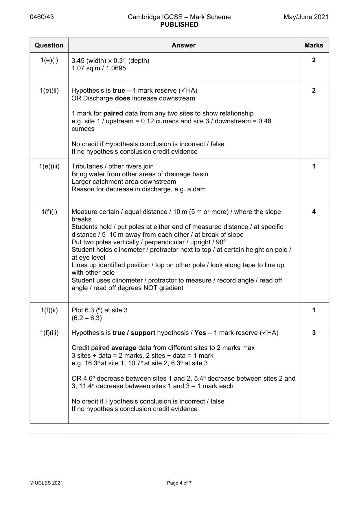
Mark scheme: Question Answer Marks 1(a)(i) Stream which joins another stream / river 1 When / where a stream joins the main river 1(a)(ii) Area drained by a river / area from where all water flows into river / 1 catchment area Area where all the rain goes into the river 1(b) Learn how to use equipment 2 Practise fieldwork techniques 2 @ 1 1(c)(i) Measure 10 metres 4 Put poles or sticks at measured distance / 10 metres along river / at start and end of measured distance Put float / orange / ball in river at start Start stopwatch or timer when float / orange is put in river Measure time it takes to travel the measured distance / stop stopwatch or timer when float reaches end of measured distance 1(c)(ii) Floats got stuck / hit obstacles / vegetation in channel 2 Error in calculation / measuring distance / measuring time Float doesn’t move in straight line Float affected by wind 2 @ 1 1(d)(i) Put measuring tape across river / channel / from one bank / side to the 4 other Keep tape measure taut / horizontal / stretched / above water / parallel to water level Measure at right angles to bank / straight across channel Read width / measurement on tape measure Rest ruler / measuring stick on river bed / bottom of river (NOT into bed) Make sure ruler is upright / vertical / straight / perpendicular / 90⁰ Measure depth at different places / intervals across channel / every metre / three points across river Read off the scale where water level reaches / where ruler is wet / measure the wet section 1 mark reserve for width and depth 1(d)(ii) 3 plots correct = 2 marks 3 1 or 2 plots correct = 1 mark Line joining points – must intersect 0 at both banks = 1 mark Ignore shading 1(e)(i) 3.45 (width) × 0.31 (depth) 2 1.07 sq m / 1.0695 1(e)(ii) Hypothesis is true – 1 mark reserve (HA) 2 OR Discharge does increase downstream 1 mark for paired data from any two sites to show relationship e.g. site 1 / upstream = 0.12 cumecs and site 3 / downstream = 0.48 cumecs No credit if Hypothesis conclusion is incorrect / false If no hypothesis conclusion credit evidence 1(e)(iii) Tributaries / other rivers join 1 Bring water from other areas of drainage basin Larger catchment area downstream Reason for decrease in discharge, e.g. a dam 1(f)(i) Measure certain / equal distance / 10 m (5 m or more) / where the slope 4 breaks Students hold / put poles at either end of measured distance / at specific distance / 5–10 m away from each other / at break of slope Put two poles vertically / perpendicular / upright / 90⁰ Student holds clinometer / protractor next to top / at certain height on pole / at eye level Lines up identified position / top on other pole / look along tape to line up with other pole Student uses clinometer / protractor to measure / record angle / read off angle / read off degrees NOT gradient 1(f)(ii) Plot 6.3 (⁰) at site 3 1 (6.2 – 6.3) 1(f)(iii) Hypothesis is true / support hypothesis / Yes – 1 mark reserve (HA) 3 Credit paired average data from different sites to 2 marks max 3 sites + data = 2 marks, 2 sites + data = 1 mark e.g. 16.3o at site 1, 10.7o at site 2, 6.3o at site 3 OR 4.6o decrease between sites 1 and 2, 5.4o decrease between sites 2 and 3, 11.4o decrease between sites 1 and 3 – 1 mark each No credit if Hypothesis conclusion is incorrect / false If no hypothesis conclusion credit evidence

More questions on Rivers

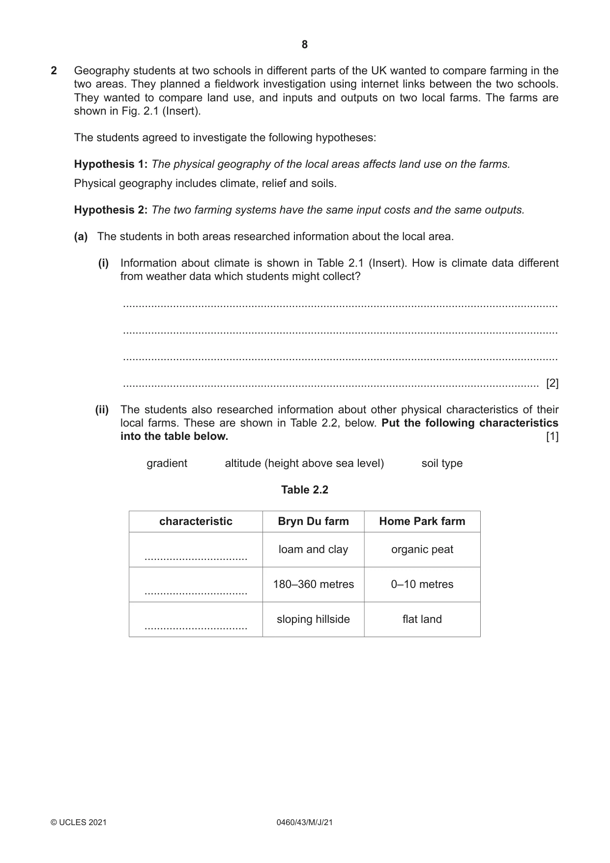
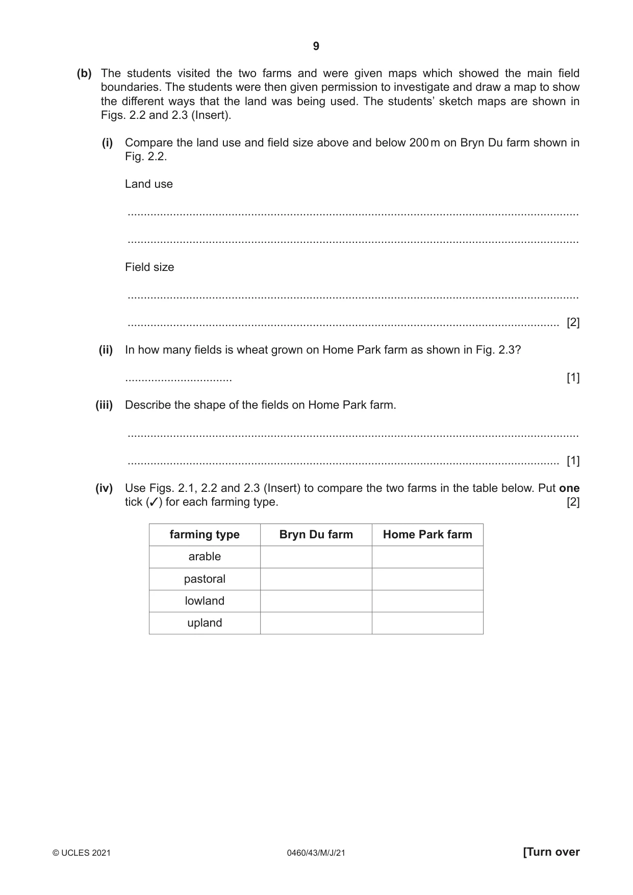
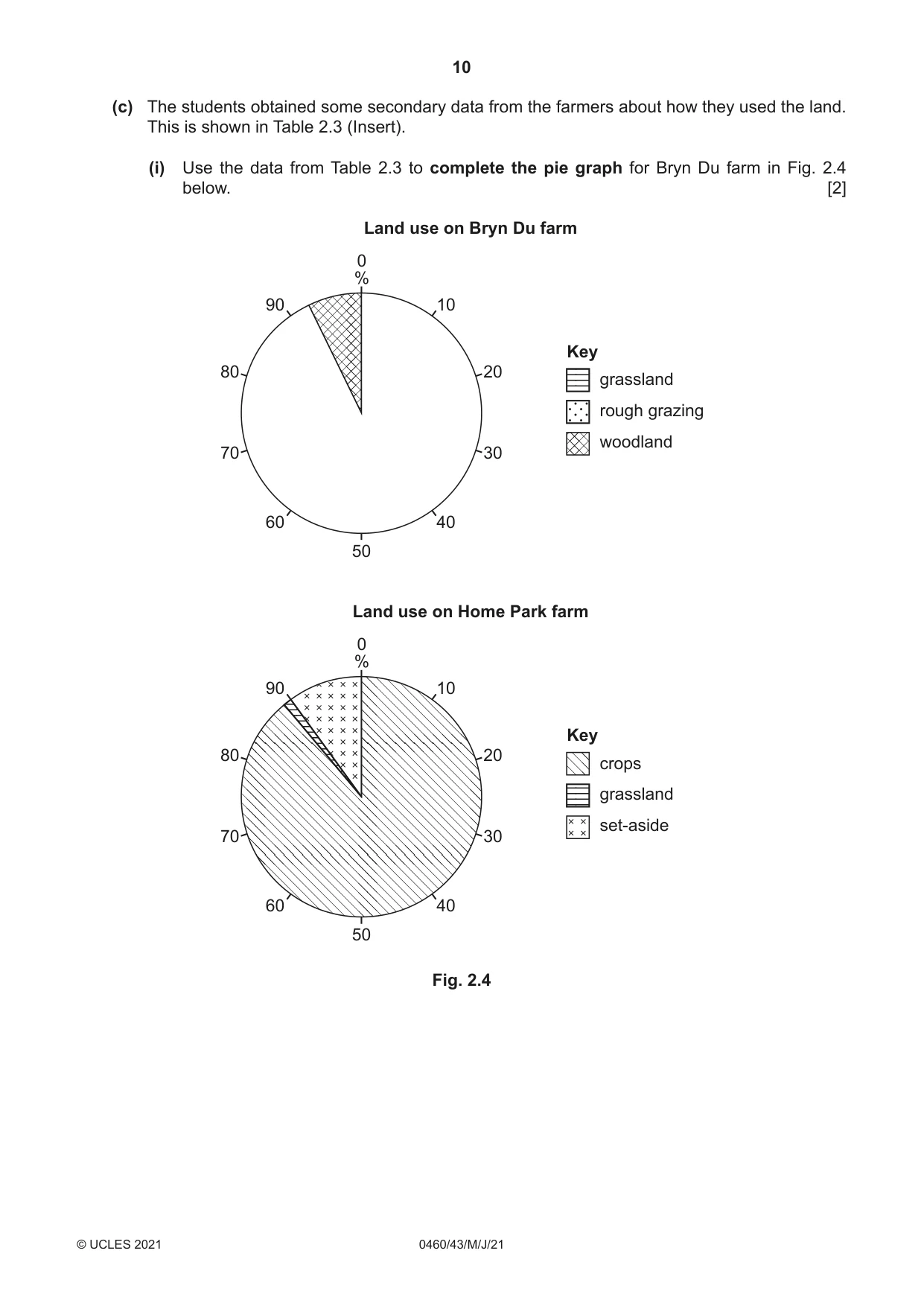
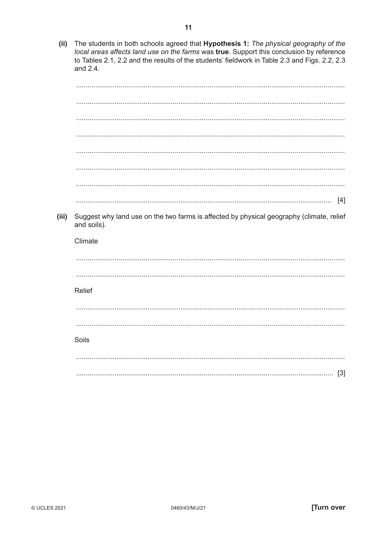
2 Geography students at two schools in different parts of the UK wanted to compare farming in the two areas. They planned a fieldwork investigation using internet links between the two schools. They wanted to compare land use, and inputs and outputs on two local farms. The farms are shown in Fig. 2.1 (Insert). The students agreed to investigate the following hypotheses: Hypothesis 1: The physical geography of the local areas affects land use on the farms. Physical geography includes climate, relief and soils. Hypothesis 2: The two farming systems have the same input costs and the same outputs. (a) The students in both areas researched information about the local area. (i) Information about climate is shown in Table 2.1 (Insert). How is climate data different from weather data which students might collect? ........................................................................................................................................... ........................................................................................................................................... ........................................................................................................................................... ..................................................................................................................................... [2] (ii) The students also researched information about other physical characteristics of their local farms. These are shown in Table 2.2, below. Put the following characteristics into the table below. [1] gradient altitude (height above sea level) soil type Table 2.2 characteristic Bryn Du farm Home Park farm loam and clay organic peat ................................. 180–360 metres 0–10 metres ................................. sloping hillside flat land ................................. (b) The students visited the two farms and were given maps which showed the main field boundaries. The students were then given permission to investigate and draw a map to show the different ways that the land was being used. The students’ sketch maps are shown in Figs. 2.2 and 2.3 (Insert). (i) Compare the land use and field size above and below 200 m on Bryn Du farm shown in Fig. 2.2. Land use ........................................................................................................................................... ........................................................................................................................................... Field size ........................................................................................................................................... ..................................................................................................................................... [2] (ii) In how many fields is wheat grown on Home Park farm as shown in Fig. 2.3? ................................. [1] (iii) Describe the shape of the fields on Home Park farm. ........................................................................................................................................... ..................................................................................................................................... [1] (iv) Use Figs. 2.1, 2.2 and 2.3 (Insert) to compare the two farms in the table below. Put one tick (✓) for each farming type. [2] farming type Bryn Du farm Home Park farm arable pastoral lowland upland (c) The students obtained some secondary data from the farmers about how they used the land. This is shown in Table 2.3 (Insert). (i) Use the data from Table 2.3 to complete the pie graph for Bryn Du farm in Fig. 2.4 below. [2] Land use on Bryn Du farm 0 % 90 10 Key 80 20 grassland rough grazing woodland 70 30 60 40 50 Land use on Home Park farm 0 % 90 10 Key 80 20 crops grassland set-aside 70 30 60 40 50 Fig. 2.4

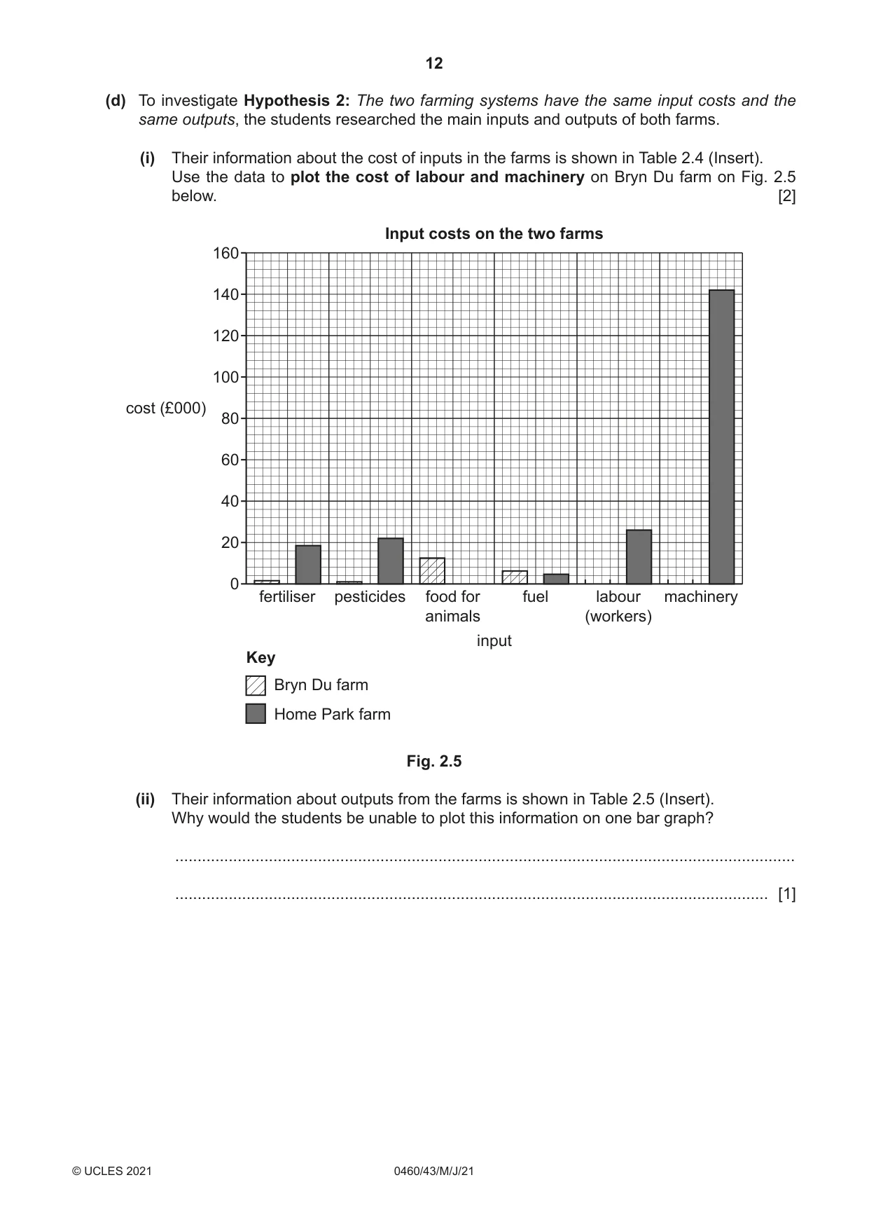
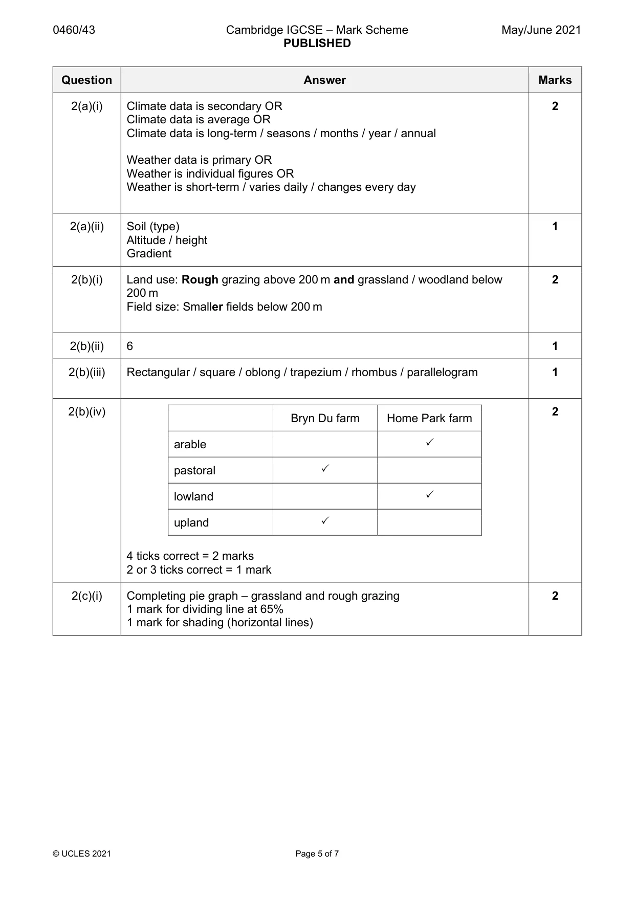
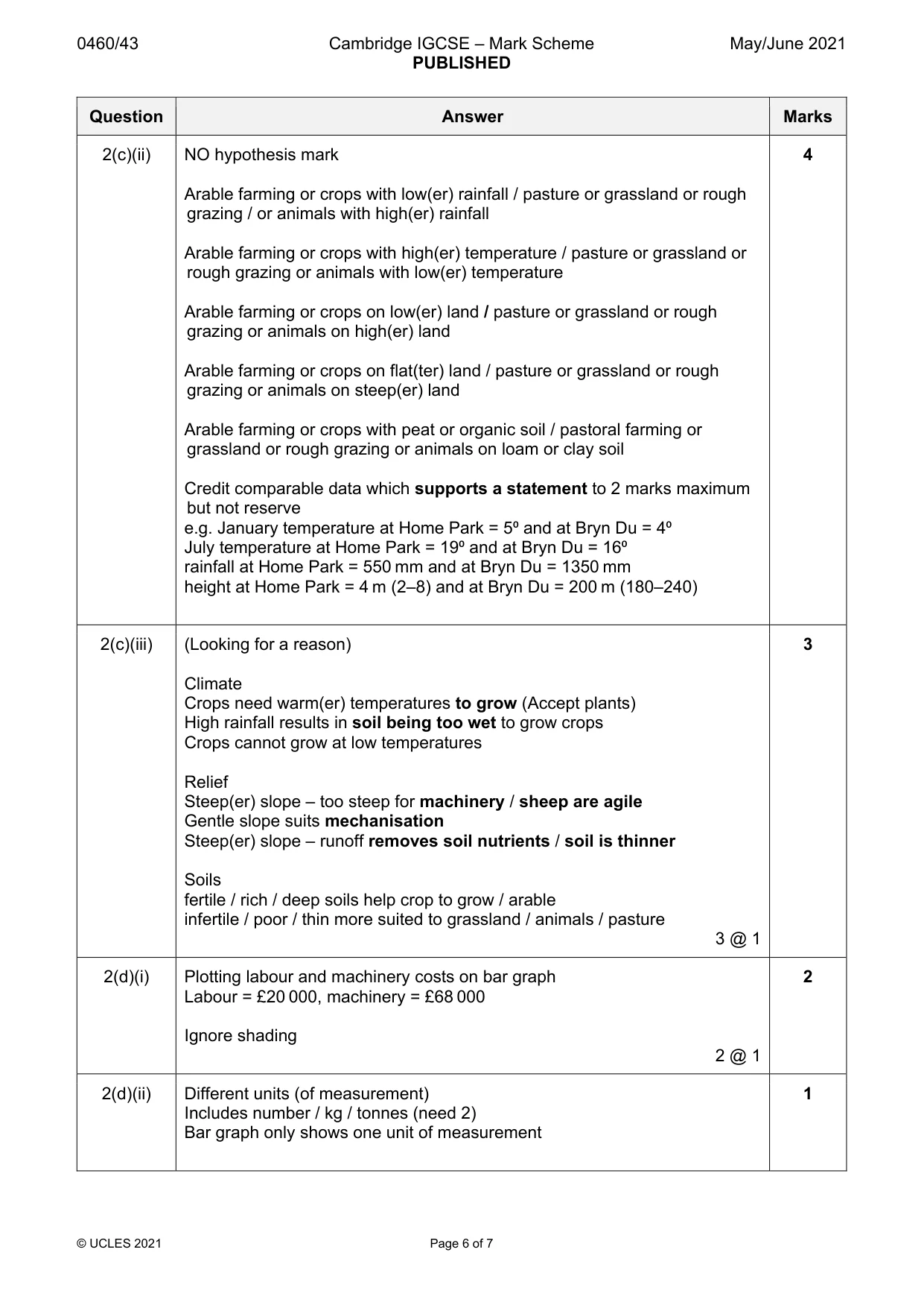
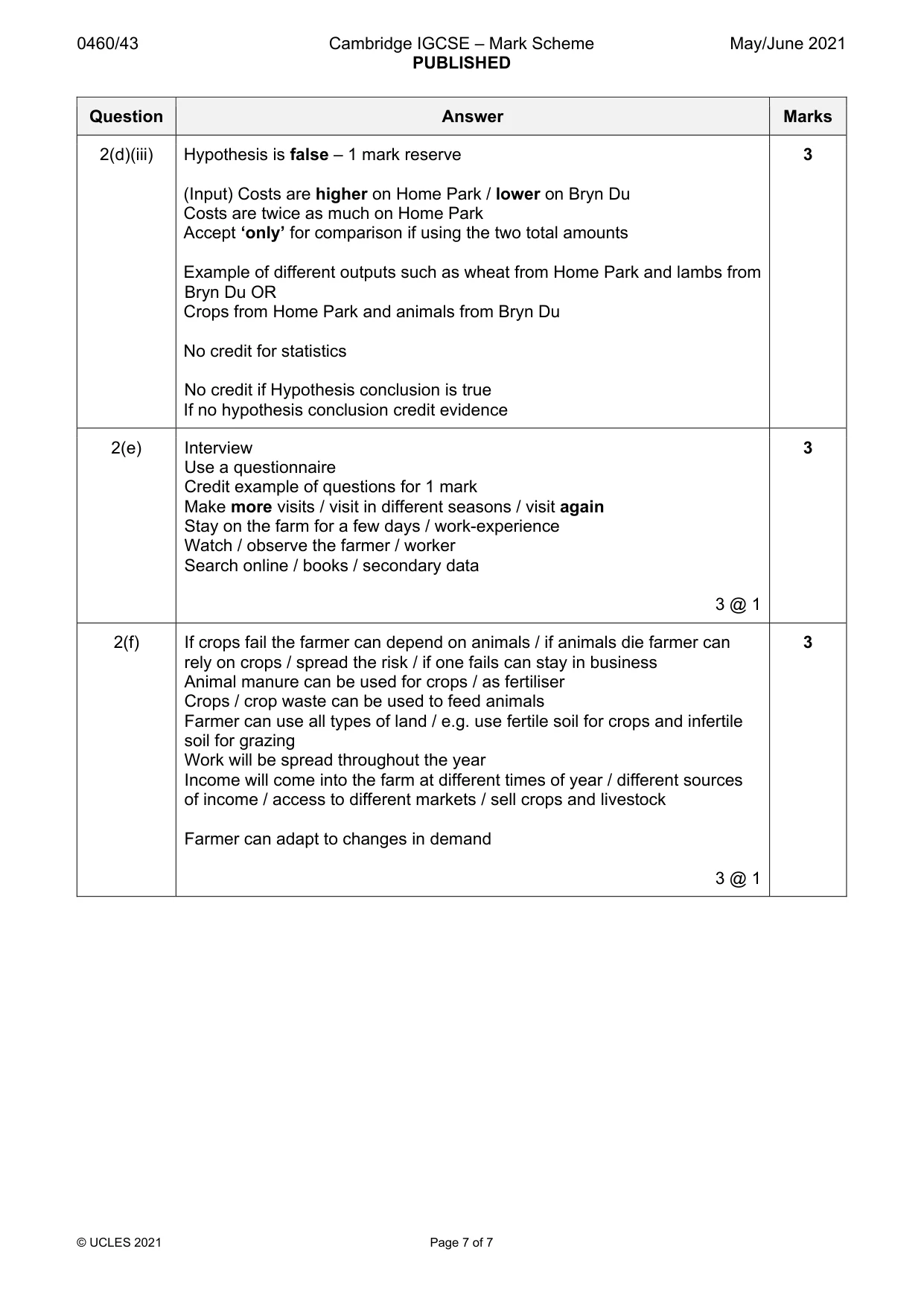
Mark scheme: 2(a)(i) Climate data is secondary OR 2 Climate data is average OR Climate data is long-term / seasons / months / year / annual Weather data is primary OR Weather is individual figures OR Weather is short-term / varies daily / changes every day 2(a)(ii) Soil (type) 1 Altitude / height Gradient 2(b)(i) Land use: Rough grazing above 200 m and grassland / woodland below 2 200 m Field size: Smaller fields below 200 m 2(b)(ii) 6 1 2(b)(iii) Rectangular / square / oblong / trapezium / rhombus / parallelogram 1 2(b)(iv) 2 Bryn Du farm Home Park farm arable  pastoral  lowland  upland  4 ticks correct = 2 marks 2 or 3 ticks correct = 1 mark 2(c)(i) Completing pie graph – grassland and rough grazing 2 1 mark for dividing line at 65% 1 mark for shading (horizontal lines) 2(c)(ii) NO hypothesis mark 4 Arable farming or crops with low(er) rainfall / pasture or grassland or rough grazing / or animals with high(er) rainfall Arable farming or crops with high(er) temperature / pasture or grassland or rough grazing or animals with low(er) temperature Arable farming or crops on low(er) land / pasture or grassland or rough grazing or animals on high(er) land Arable farming or crops on flat(ter) land / pasture or grassland or rough grazing or animals on steep(er) land Arable farming or crops with peat or organic soil / pastoral farming or grassland or rough grazing or animals on loam or clay soil Credit comparable data which supports a statement to 2 marks maximum but not reserve e.g. January temperature at Home Park = 5⁰ and at Bryn Du = 4⁰ July temperature at Home Park = 19⁰ and at Bryn Du = 16⁰ rainfall at Home Park = 550 mm and at Bryn Du = 1350 mm height at Home Park = 4 m (2–8) and at Bryn Du = 200 m (180–240) 2(c)(iii) (Looking for a reason) 3 Climate Crops need warm(er) temperatures to grow (Accept plants) High rainfall results in soil being too wet to grow crops Crops cannot grow at low temperatures Relief Steep(er) slope – too steep for machinery / sheep are agile Gentle slope suits mechanisation Steep(er) slope – runoff removes soil nutrients / soil is thinner Soils fertile / rich / deep soils help crop to grow / arable infertile / poor / thin more suited to grassland / animals / pasture 3 @ 1 2(d)(i) Plotting labour and machinery costs on bar graph 2 Labour = £20 000, machinery = £68 000 Ignore shading 2 @ 1 2(d)(ii) Different units (of measurement) 1 Includes number / kg / tonnes (need 2) Bar graph only shows one unit of measurement 2(d)(iii) Hypothesis is false – 1 mark reserve 3 (Input) Costs are higher on Home Park / lower on Bryn Du Costs are twice as much on Home Park Accept ‘only’ for comparison if using the two total amounts Example of different outputs such as wheat from Home Park and lambs from Bryn Du OR Crops from Home Park and animals from Bryn Du No credit for statistics No credit if Hypothesis conclusion is true If no hypothesis conclusion credit evidence 2(e) Interview 3 Use a questionnaire Credit example of questions for 1 mark Make more visits / visit in different seasons / visit again Stay on the farm for a few days / work-experience Watch / observe the farmer / worker Search online / books / secondary data 3 @ 1 2(f) If crops fail the farmer can depend on animals / if animals die farmer can 3 rely on crops / spread the risk / if one fails can stay in business Animal manure can be used for crops / as fertiliser Crops / crop waste can be used to feed animals Farmer can use all types of land / e.g. use fertile soil for crops and infertile soil for grazing Work will be spread throughout the year Income will come into the farm at different times of year / different sources of income / access to different markets / sell crops and livestock Farmer can adapt to changes in demand 3 @ 1

More questions on Food production