Cambridge IGCSE Geography 0460 — 2019 May/June Paper 4 · Variant 2

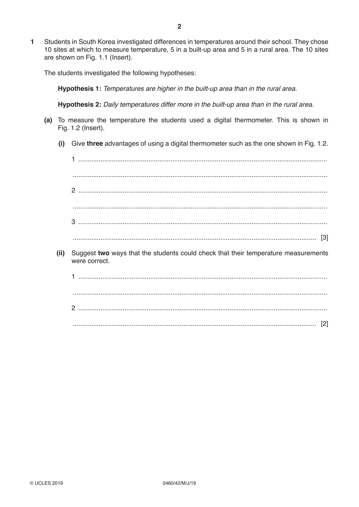
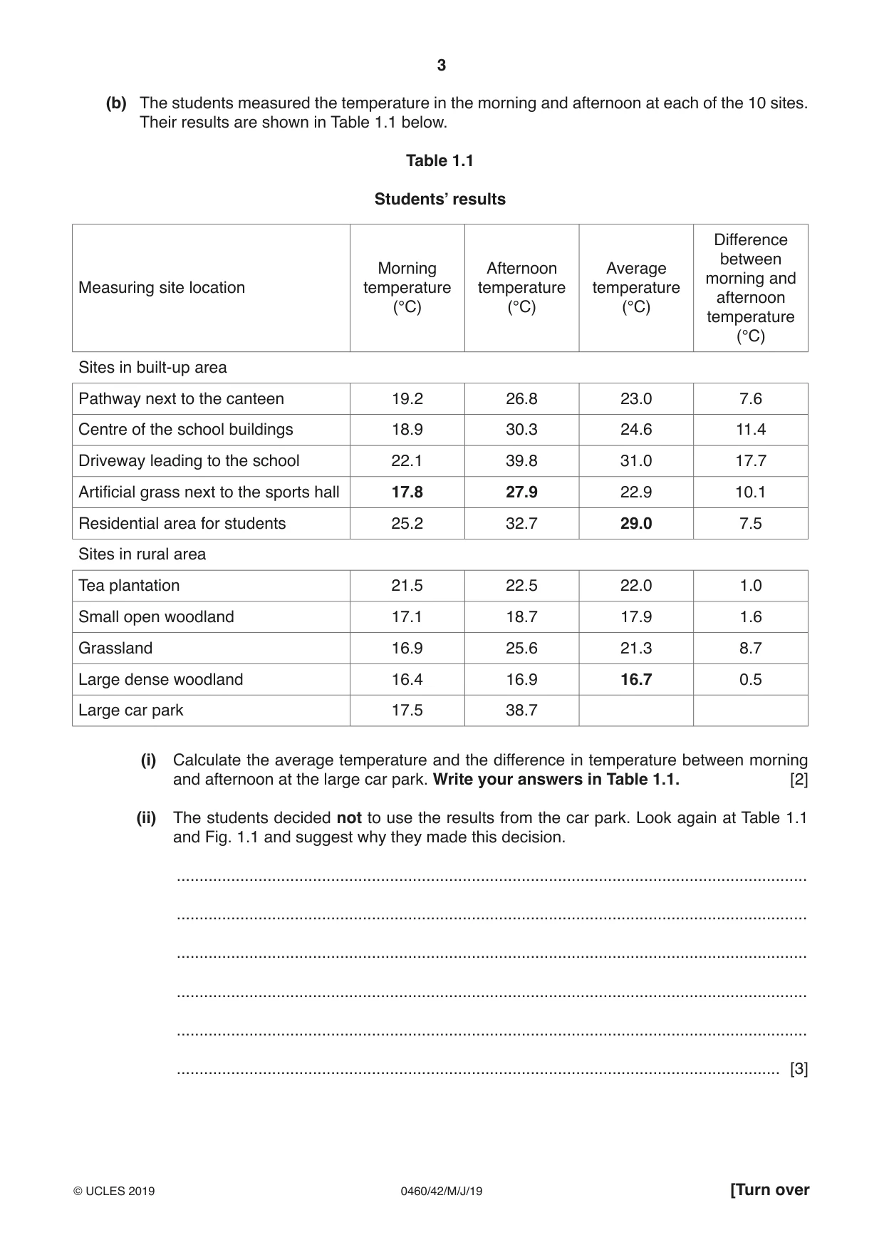
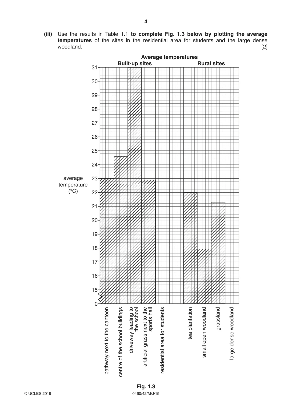
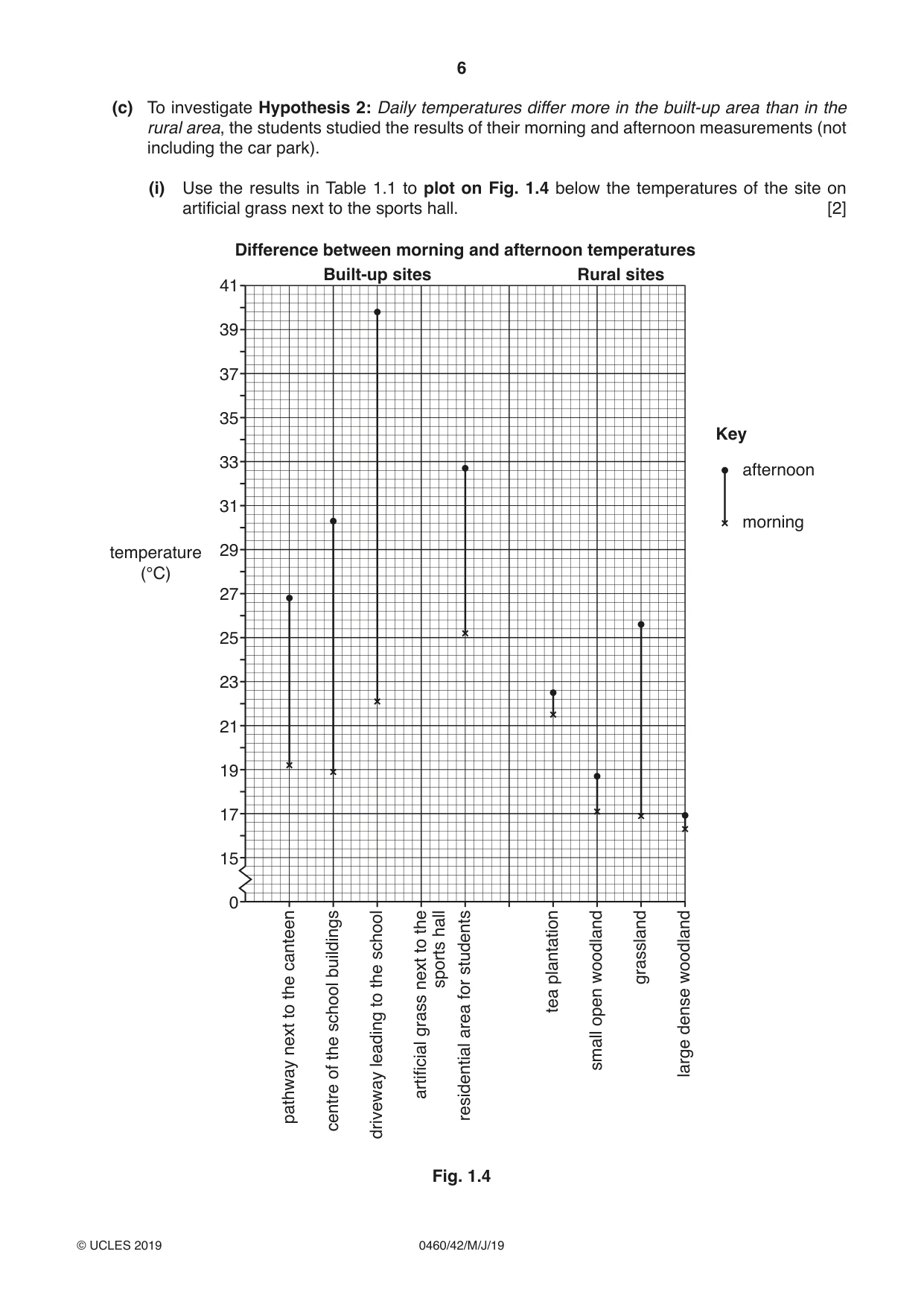
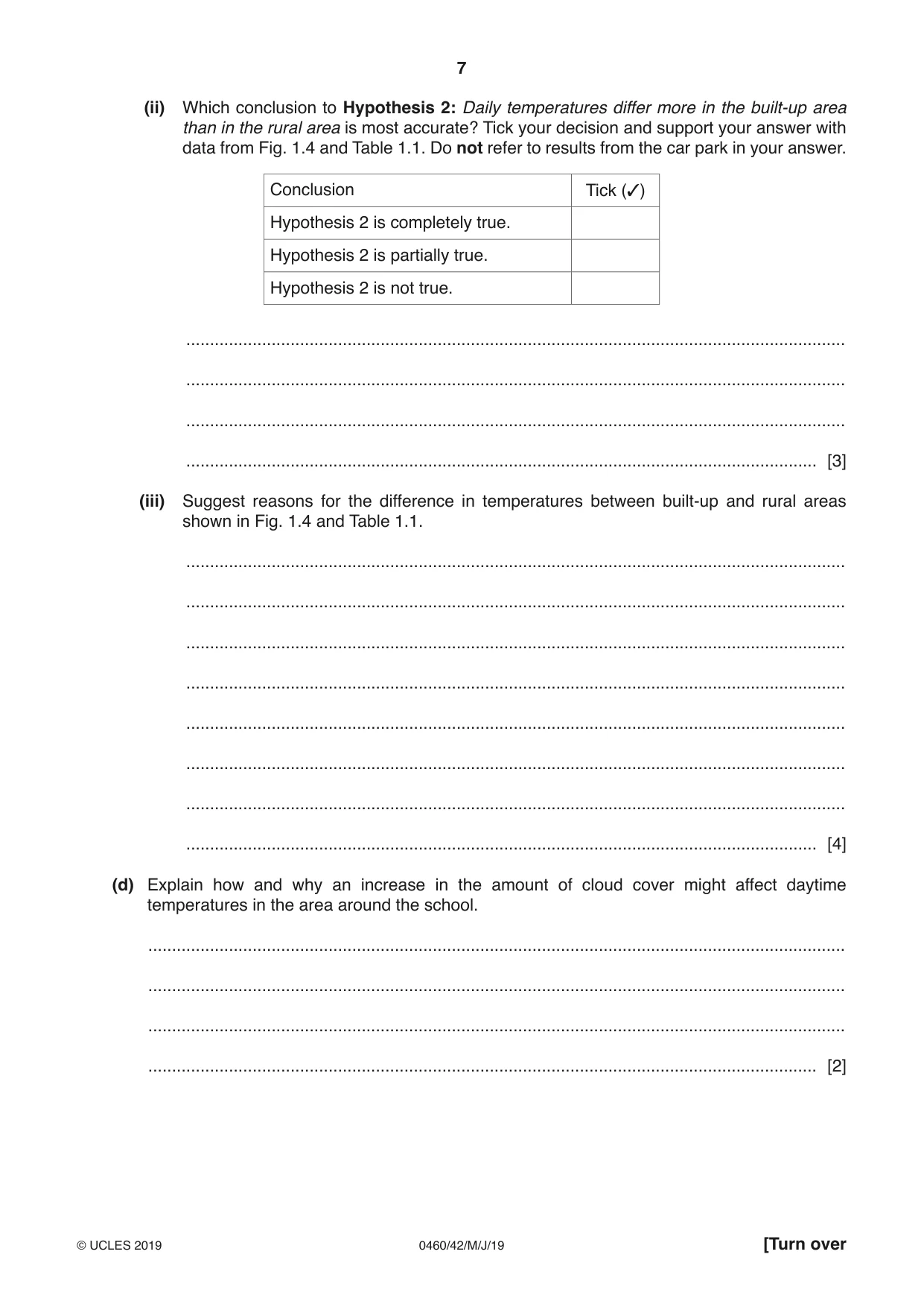
1 Students in South Korea investigated differences in temperatures around their school. They chose 10 sites at which to measure temperature, 5 in a built-up area and 5 in a rural area. The 10 sites are shown on Fig. 1.1 (Insert). The students investigated the following hypotheses: Hypothesis 1: Temperatures are higher in the built-up area than in the rural area. Hypothesis 2: Daily temperatures differ more in the built-up area than in the rural area. (a) To measure the temperature the students used a digital thermometer. This is shown in Fig. 1.2 (Insert). (i) Give three advantages of using a digital thermometer such as the one shown in Fig. 1.2. 1 ....................................................................................................................................... .......................................................................................................................................... 2 ....................................................................................................................................... .......................................................................................................................................... 3 ....................................................................................................................................... .................................................................................................................................... [3] (ii) Suggest two ways that the students could check that their temperature measurements were correct. 1 ....................................................................................................................................... .......................................................................................................................................... 2 ....................................................................................................................................... .................................................................................................................................... [2] (b) The students measured the temperature in the morning and afternoon at each of the 10 sites. Their results are shown in Table 1.1 below. Table 1.1 Students’ results Difference between Morning Afternoon Average morning andMeasuring site location temperature temperature temperature afternoon (°C) (°C) (°C) temperature (°C) Sites in built-up area Pathway next to the canteen 19.2 26.8 23.0 7.6 Centre of the school buildings 18.9 30.3 24.6 11.4 Driveway leading to the school 22.1 39.8 31.0 17.7 Artificial grass next to the sports hall 17.8 27.9 22.9 10.1 Residential area for students 25.2 32.7 29.0 7.5 Sites in rural area Tea plantation 21.5 22.5 22.0 1.0 Small open woodland 17.1 18.7 17.9 1.6 Grassland 16.9 25.6 21.3 8.7 Large dense woodland 16.4 16.9 16.7 0.5 Large car park 17.5 38.7 (i) Calculate the average temperature and the difference in temperature between morning and afternoon at the large car park. Write your answers in Table 1.1. [2] (ii) The students decided not to use the results from the car park. Look again at Table 1.1 and Fig. 1.1 and suggest why they made this decision. ........................................................................................................................................... ........................................................................................................................................... ........................................................................................................................................... ........................................................................................................................................... ........................................................................................................................................... ..................................................................................................................................... [3] (iii) Use the results in Table 1.1 to complete Fig. 1.3 below by plotting the average temperatures of the sites in the residential area for students and the large dense woodland. [2] Average temperatures Built-up sites Rural sites 31 30 29 28 27 26 25 24 average 23 temperature (°C) 22 21 20 19 18 17 16 15 0 to thehall to school canteen buildings leading students plantation woodland grassland woodland thenextsports the for tea to open school grass area dense next the driveway small of artificial residential large pathway centre Fig. 1.3 (iv) What is your conclusion to Hypothesis 1: Temperatures are higher in the built-up area than in the rural area? Support your decision with evidence from Fig. 1.3 and Table 1.1. Do not refer to results from the car park in your answer. ........................................................................................................................................... ........................................................................................................................................... ........................................................................................................................................... ........................................................................................................................................... ........................................................................................................................................... ..................................................................................................................................... [3] (c) To investigate Hypothesis 2: Daily temperatures differ more in the built-up area than in the rural area, the students studied the results of their morning and afternoon measurements (not including the car park). (i) Use the results in Table 1.1 to plot on Fig. 1.4 below the temperatures of the site on artificial grass next to the sports hall. [2] Difference between morning and afternoon temperatures Built-up sites Rural sites 41 39 37 35 Key 33 afternoon 31 morning temperature 29 (°C) 27 25 23 21 19 17 15 0 thehall to canteen buildings school students plantation woodland grassland woodland the nextsports the for to tea to open school grass area dense next the leading small of artificial residential large pathway centre driveway Fig. 1.4 (ii) Which conclusion to Hypothesis 2: Daily temperatures differ more in the built-up area than in the rural area is most accurate? Tick your decision and support your answer with data from Fig. 1.4 and Table 1.1. Do not refer to results from the car park in your answer. Conclusion Tick (3) Hypothesis 2 is completely true. Hypothesis 2 is partially true. Hypothesis 2 is not true. ........................................................................................................................................... ........................................................................................................................................... ........................................................................................................................................... ..................................................................................................................................... [3] (iii) Suggest reasons for the difference in temperatures between built-up and rural areas shown in Fig. 1.4 and Table 1.1. ........................................................................................................................................... ........................................................................................................................................... ........................................................................................................................................... ........................................................................................................................................... ........................................................................................................................................... ........................................................................................................................................... ........................................................................................................................................... ..................................................................................................................................... [4] (d) Explain how and why an increase in the amount of cloud cover might affect daytime temperatures in the area around the school. ................................................................................................................................................... ................................................................................................................................................... ................................................................................................................................................... ............................................................................................................................................. [2] (e) Whilst measuring the temperatures at different sites the students realised that wind speed varied. An instrument to measure wind speed is shown in Fig. 1.5 (Insert). (i) What is the instrument used to measure wind speed called? .............................................................. [1] (ii) Explain how this instrument measures wind speed. ........................................................................................................................................... ........................................................................................................................................... ........................................................................................................................................... ........................................................................................................................................... ........................................................................................................................................... ..................................................................................................................................... [3] [Total: 30]

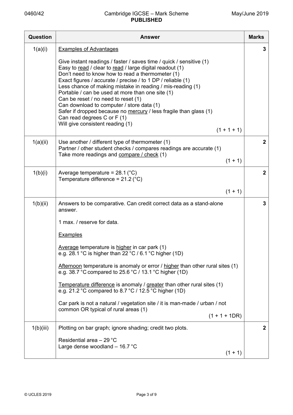
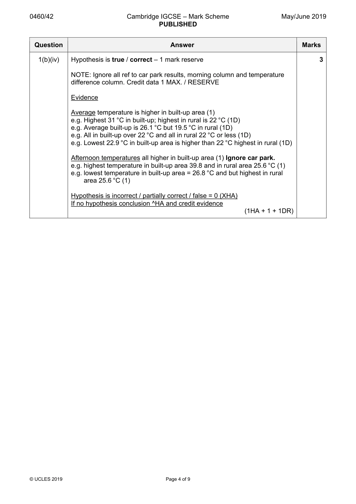
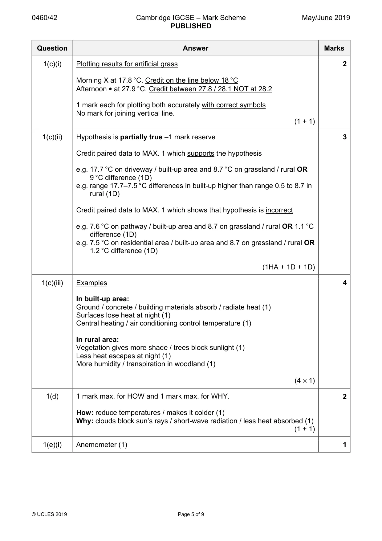
Mark scheme: Question Answer Marks 1(a)(i) Examples of Advantages 3 Give instant readings / faster / saves time / quick / sensitive (1) Easy to read / clear to read / large digital readout (1) Don’t need to know how to read a thermometer (1) Exact figures / accurate / precise / to 1 DP / reliable (1) Less chance of making mistake in reading / mis-reading (1) Portable / can be used at more than one site (1) Can be reset / no need to reset (1) Can download to computer / store data (1) Safer if dropped because no mercury / less fragile than glass (1) Can read degrees C or F (1) Will give consistent reading (1) (1 + 1 + 1) 1(a)(ii) Use another / different type of thermometer (1) 2 Partner / other student checks / compares readings are accurate (1) Take more readings and compare / check (1) (1 + 1) 1(b)(i) Average temperature = 28.1 (°C) 2 Temperature difference = 21.2 (°C) (1 + 1) 1(b)(ii) Answers to be comparative. Can credit correct data as a stand-alone 3 answer. 1 max. / reserve for data. Examples Average temperature is higher in car park (1) e.g. 28.1 °C is higher than 22 °C / 6.1 °C higher (1D) Afternoon temperature is anomaly or error / higher than other rural sites (1) e.g. 38.7 °C compared to 25.6 °C / 13.1 °C higher (1D) Temperature difference is anomaly / greater than other rural sites (1) e.g. 21.2 °C compared to 8.7 °C / 12.5 °C higher (1D) Car park is not a natural / vegetation site / it is man-made / urban / not common OR typical of rural areas (1) (1 + 1 + 1DR) 1(b)(iii) Plotting on bar graph; ignore shading; credit two plots. 2 Residential area – 29 °C Large dense woodland – 16.7 °C (1 + 1) 1(b)(iv) Hypothesis is true / correct – 1 mark reserve 3 NOTE: Ignore all ref to car park results, morning column and temperature difference column. Credit data 1 MAX. / RESERVE Evidence Average temperature is higher in built-up area (1) e.g. Highest 31 °C in built-up; highest in rural is 22 °C (1D) e.g. Average built-up is 26.1 °C but 19.5 °C in rural (1D) e.g. All in built-up over 22 °C and all in rural 22 °C or less (1D) e.g. Lowest 22.9 °C in built-up area is higher than 22 °C highest in rural (1D) Afternoon temperatures all higher in built-up area (1) Ignore car park. e.g. highest temperature in built-up area 39.8 and in rural area 25.6 °C (1) e.g. lowest temperature in built-up area = 26.8 °C and but highest in rural area 25.6 °C (1) Hypothesis is incorrect / partially correct / false = 0 (XHA) If no hypothesis conclusion ^HA and credit evidence (1HA + 1 + 1DR) 1(c)(i) Plotting results for artificial grass 2 Morning X at 17.8 °C. Credit on the line below 18 °C Afternoon • at 27.9 °C. Credit between 27.8 / 28.1 NOT at 28.2 1 mark each for plotting both accurately with correct symbols No mark for joining vertical line. (1 + 1) 1(c)(ii) Hypothesis is partially true –1 mark reserve 3 Credit paired data to MAX. 1 which supports the hypothesis e.g. 17.7 °C on driveway / built-up area and 8.7 °C on grassland / rural OR 9 °C difference (1D) e.g. range 17.7–7.5 °C differences in built-up higher than range 0.5 to 8.7 in rural (1D) Credit paired data to MAX. 1 which shows that hypothesis is incorrect e.g. 7.6 °C on pathway / built-up area and 8.7 on grassland / rural OR 1.1 °C difference (1D) e.g. 7.5 °C on residential area / built-up area and 8.7 on grassland / rural OR 1.2 °C difference (1D) (1HA + 1D + 1D) 1(c)(iii) Examples 4 In built-up area: Ground / concrete / building materials absorb / radiate heat (1) Surfaces lose heat at night (1) Central heating / air conditioning control temperature (1) In rural area: Vegetation gives more shade / trees block sunlight (1) Less heat escapes at night (1) More humidity / transpiration in woodland (1) (4 × 1) 1(d) 1 mark max. for HOW and 1 mark max. for WHY. 2 How: reduce temperatures / makes it colder (1) Why: clouds block sun’s rays / short-wave radiation / less heat absorbed (1) (1 + 1) 1(e)(i) Anemometer (1) 1 1(e)(ii) Examples 3 • Cups / cones / arms / wings / blades revolve / spin / rotate / turn / pushed around / circular motion (1) Must name part that spins etc.; • Meter counts / records number of revolutions / counts or records • wind speed (1) • Display screen shows wind speed / number (1) • Reading as kms per hour (1) (3 × 1)

More questions on Weather

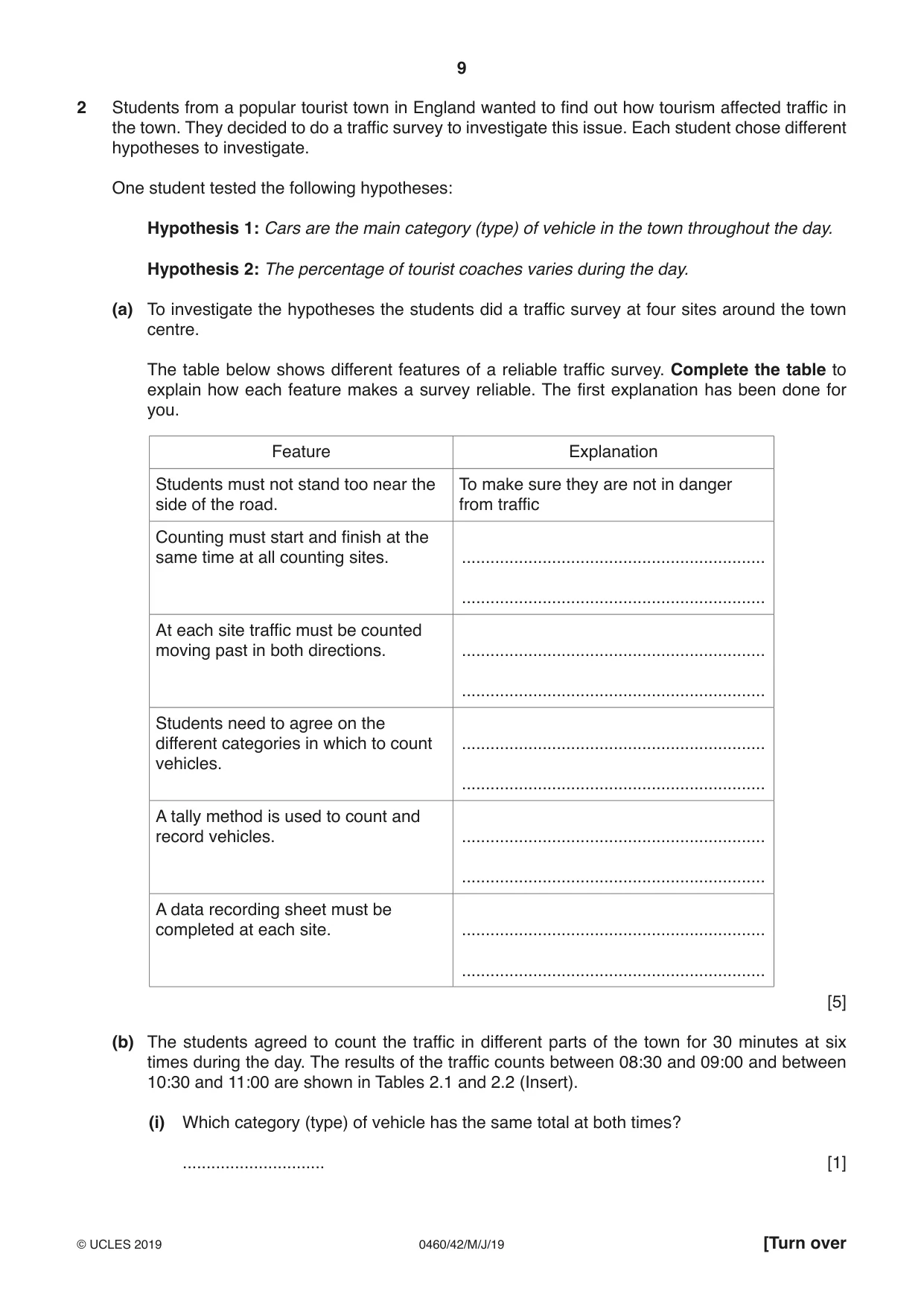
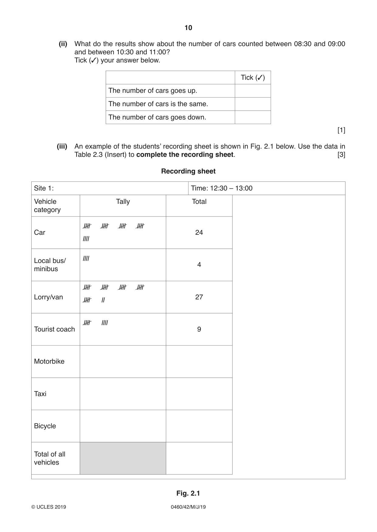
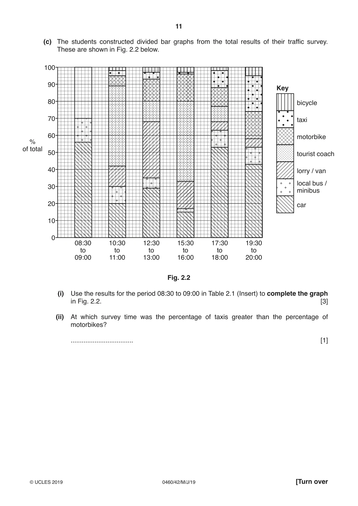
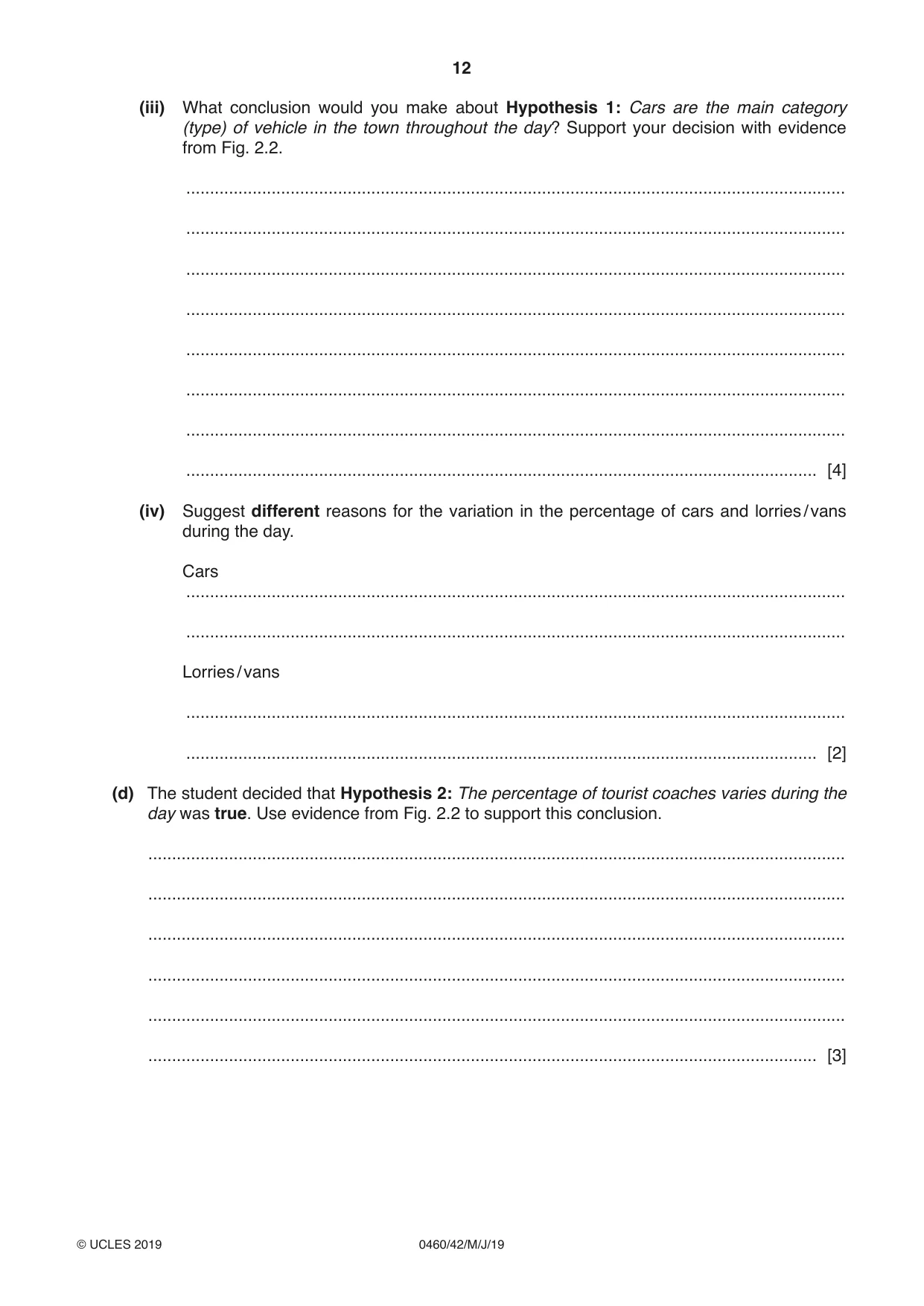
2 Students from a popular tourist town in England wanted to find out how tourism affected traffic in the town. They decided to do a traffic survey to investigate this issue. Each student chose different hypotheses to investigate. One student tested the following hypotheses: Hypothesis 1: Cars are the main category (type) of vehicle in the town throughout the day. Hypothesis 2: The percentage of tourist coaches varies during the day. (a) To investigate the hypotheses the students did a traffic survey at four sites around the town centre. The table below shows different features of a reliable traffic survey. Complete the table to explain how each feature makes a survey reliable. The first explanation has been done for you. Feature Explanation Students must not stand too near the To make sure they are not in danger side of the road. from traffic Counting must start and finish at the same time at all counting sites. ................................................................ ................................................................ At each site traffic must be counted moving past in both directions. ................................................................ ................................................................ Students need to agree on the different categories in which to count ................................................................ vehicles. ................................................................ A tally method is used to count and record vehicles. ................................................................ ................................................................ A data recording sheet must be completed at each site. ................................................................ ................................................................ [5] (b) The students agreed to count the traffic in different parts of the town for 30 minutes at six times during the day. The results of the traffic counts between 08:30 and 09:00 and between 10:30 and 11:00 are shown in Tables 2.1 and 2.2 (Insert). (i) Which category (type) of vehicle has the same total at both times? .............................. [1] (ii) What do the results show about the number of cars counted between 08:30 and 09:00 and between 10:30 and 11:00? Tick (3) your answer below. Tick (3) The number of cars goes up. The number of cars is the same. The number of cars goes down. [1] (iii) An example of the students’ recording sheet is shown in Fig. 2.1 below. Use the data in Table 2.3 (Insert) to complete the recording sheet. [3] Recording sheet Site 1: Time: 12:30 – 13:00 Vehicle Tally Total category llll llll llll llll Car 24 llll llllLocal bus/ 4minibus llll llll llll llll Lorry/van 27 llll ll llll llll Tourist coach 9 Motorbike Taxi Bicycle Total of all vehicles Fig. 2.1 (c) The students constructed divided bar graphs from the total results of their traffic survey. These are shown in Fig. 2.2 below. 100 90 Key 80 bicycle 70 taxi 60 motorbike % of total 50 tourist coach 40 lorry / van local bus / 30 minibus 20 car 10 0 08:30 10:30 12:30 15:30 17:30 19:30 to to to to to to 09:00 11:00 13:00 16:00 18:00 20:00 Fig. 2.2 (i) Use the results for the period 08:30 to 09:00 in Table 2.1 (Insert) to complete the graph in Fig. 2.2. [3] (ii) At which survey time was the percentage of taxis greater than the percentage of motorbikes? .................................. [1]

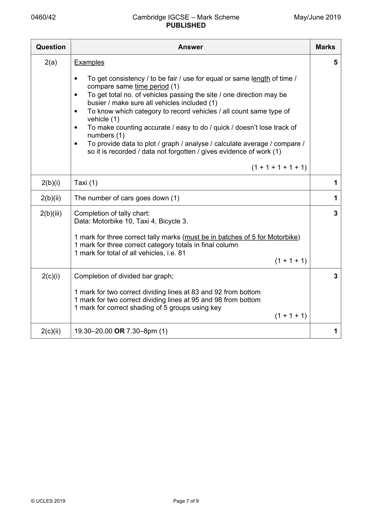
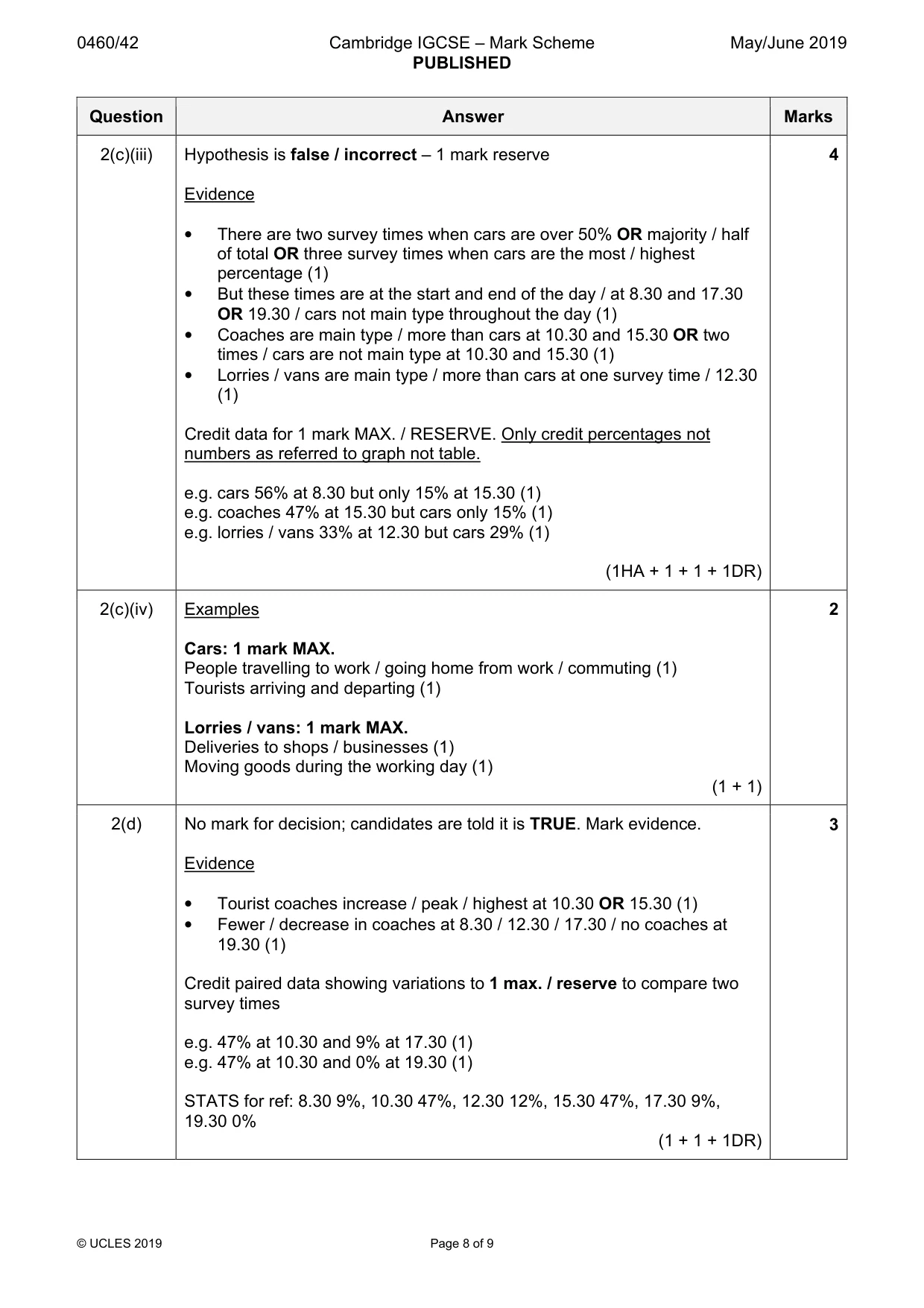
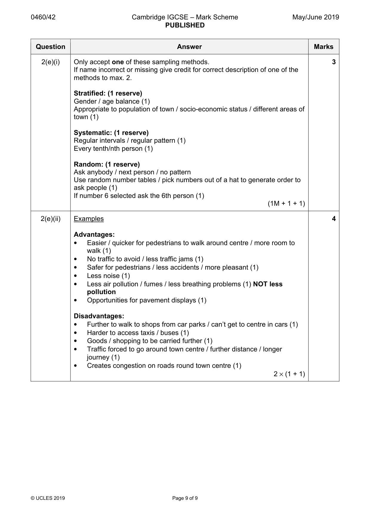
Mark scheme: 2(a) Examples 5 • To get consistency / to be fair / use for equal or same length of time / compare same time period (1) • To get total no. of vehicles passing the site / one direction may be busier / make sure all vehicles included (1) • To know which category to record vehicles / all count same type of vehicle (1) • To make counting accurate / easy to do / quick / doesn’t lose track of numbers (1) • To provide data to plot / graph / analyse / calculate average / compare / so it is recorded / data not forgotten / gives evidence of work (1) (1 + 1 + 1 + 1 + 1) 2(b)(i) Taxi (1) 1 2(b)(ii) The number of cars goes down (1) 1 2(b)(iii) Completion of tally chart: 3 Data: Motorbike 10, Taxi 4, Bicycle 3. 1 mark for three correct tally marks (must be in batches of 5 for Motorbike) 1 mark for three correct category totals in final column 1 mark for total of all vehicles, i.e. 81 (1 + 1 + 1) 2(c)(i) Completion of divided bar graph; 3 1 mark for two correct dividing lines at 83 and 92 from bottom 1 mark for two correct dividing lines at 95 and 98 from bottom 1 mark for correct shading of 5 groups using key (1 + 1 + 1) 2(c)(ii) 19.30–20.00 OR 7.30–8pm (1) 1 2(c)(iii) Hypothesis is false / incorrect – 1 mark reserve 4 Evidence • There are two survey times when cars are over 50% OR majority / half of total OR three survey times when cars are the most / highest percentage (1) • But these times are at the start and end of the day / at 8.30 and 17.30 OR 19.30 / cars not main type throughout the day (1) • Coaches are main type / more than cars at 10.30 and 15.30 OR two times / cars are not main type at 10.30 and 15.30 (1) • Lorries / vans are main type / more than cars at one survey time / 12.30 (1) Credit data for 1 mark MAX. / RESERVE. Only credit percentages not numbers as referred to graph not table. e.g. cars 56% at 8.30 but only 15% at 15.30 (1) e.g. coaches 47% at 15.30 but cars only 15% (1) e.g. lorries / vans 33% at 12.30 but cars 29% (1) (1HA + 1 + 1 + 1DR) 2(c)(iv) Examples 2 Cars: 1 mark MAX. People travelling to work / going home from work / commuting (1) Tourists arriving and departing (1) Lorries / vans: 1 mark MAX. Deliveries to shops / businesses (1) Moving goods during the working day (1) (1 + 1) 2(d) No mark for decision; candidates are told it is TRUE. Mark evidence. 3 Evidence • Tourist coaches increase / peak / highest at 10.30 OR 15.30 (1) • Fewer / decrease in coaches at 8.30 / 12.30 / 17.30 / no coaches at 19.30 (1) Credit paired data showing variations to 1 max. / reserve to compare two survey times e.g. 47% at 10.30 and 9% at 17.30 (1) e.g. 47% at 10.30 and 0% at 19.30 (1) STATS for ref: 8.30 9%, 10.30 47%, 12.30 12%, 15.30 47%, 17.30 9%, 19.30 0% (1 + 1 + 1DR) 2(e)(i) Only accept one of these sampling methods. 3 If name incorrect or missing give credit for correct description of one of the methods to max. 2. Stratified: (1 reserve) Gender / age balance (1) Appropriate to population of town / socio-economic status / different areas of town (1) Systematic: (1 reserve) Regular intervals / regular pattern (1) Every tenth/nth person (1) Random: (1 reserve) Ask anybody / next person / no pattern Use random number tables / pick numbers out of a hat to generate order to ask people (1) If number 6 selected ask the 6th person (1) (1M + 1 + 1) 2(e)(ii) Examples 4 Advantages: • Easier / quicker for pedestrians to walk around centre / more room to walk (1) • No traffic to avoid / less traffic jams (1) • Safer for pedestrians / less accidents / more pleasant (1) • Less noise (1) • Less air pollution / fumes / less breathing problems (1) NOT less pollution • Opportunities for pavement displays (1) Disadvantages: • Further to walk to shops from car parks / can’t get to centre in cars (1) • Harder to access taxis / buses (1) • Goods / shopping to be carried further (1) • Traffic forced to go around town centre / further distance / longer journey (1) • Creates congestion on roads round town centre (1) 2 × (1 + 1)

More questions on Urban settlements