Questions as text
Q1 · Conducting putty is a soft material which can easily be made into different shapes 9702/51 May/June 2007
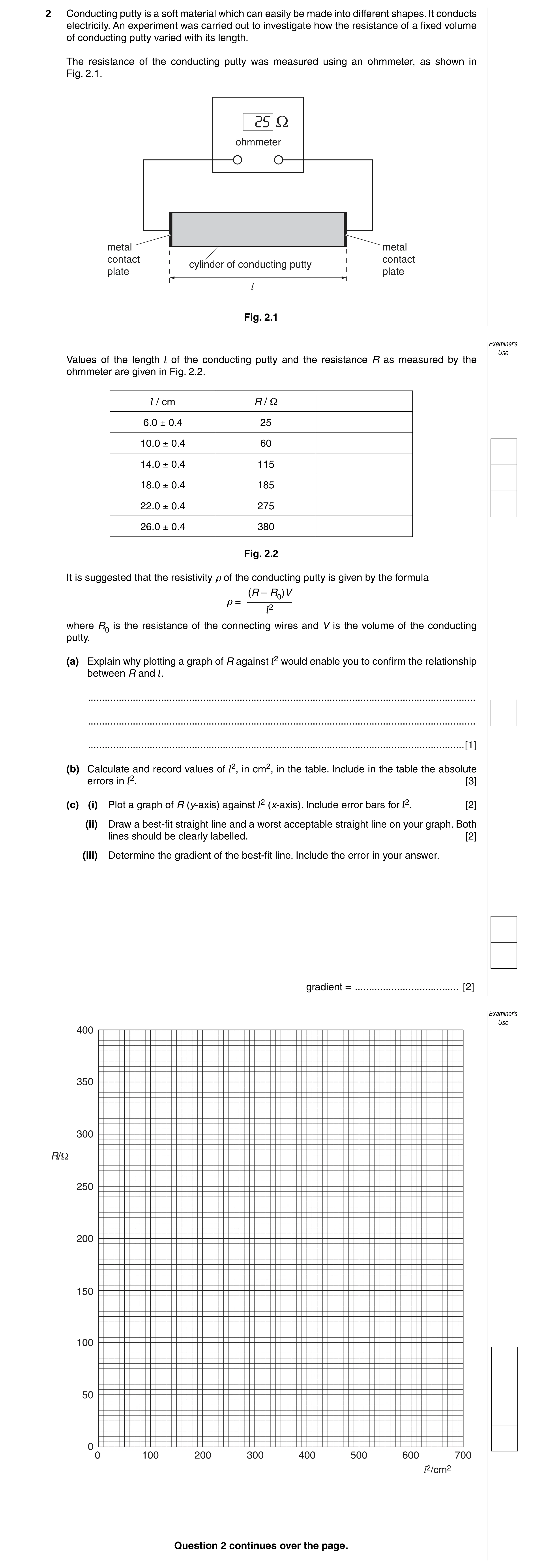
2 Conducting putty is a soft material which can easily be made into different shapes. It conducts electricity. An experiment was carried out to investigate how the resistance of a fixed volume of conducting putty varied with its length. The resistance of the conducting putty was measured using an ohmmeter, as shown in Fig. 2.1. ohmmeter metal metal contact contact cylinder of conducting putty plate plate l Fig. 2.1 Examiner’s Use Values of the length l of the conducting putty and the resistance R as measured by the ohmmeter are given in Fig. 2.2. l / cm R / Ω 6.0 ± 0.4 25 10.0 ± 0.4 60 14.0 ± 0.4 115 18.0 ± 0.4 185 22.0 ± 0.4 275 26.0 ± 0.4 380 Fig. 2.2 It is suggested that the resistivity ρ of the conducting putty is given by the formula (R – R0)V ________ ρ = l2 where R0 is the resistance of the connecting wires and V is the volume of the conducting putty. (a) Explain why plotting a graph of R against l2 would enable you to confirm the relationship between R and l. … … … [1] (b) Calculate and record values of l2, in cm2, in the table. Include in the table the absolute errors in l2. [3] (c) (i) Plot a graph of R (y-axis) against l2 (x-axis). Include error bars for l2. [2] (ii) Draw a best-fit straight line and a worst acceptable straight line on your graph. Both lines should be clearly labelled. [2] (iii) Determine the gradient of the best-fit line. Include the error in your answer. gradient = … [2] Examiner’s Use 400 350 300 R/Ω 250 200 150 100 50 0 0 100 200 300 400 500 600 700 l2/cm2 Question 2 continues over the page.
10 marks
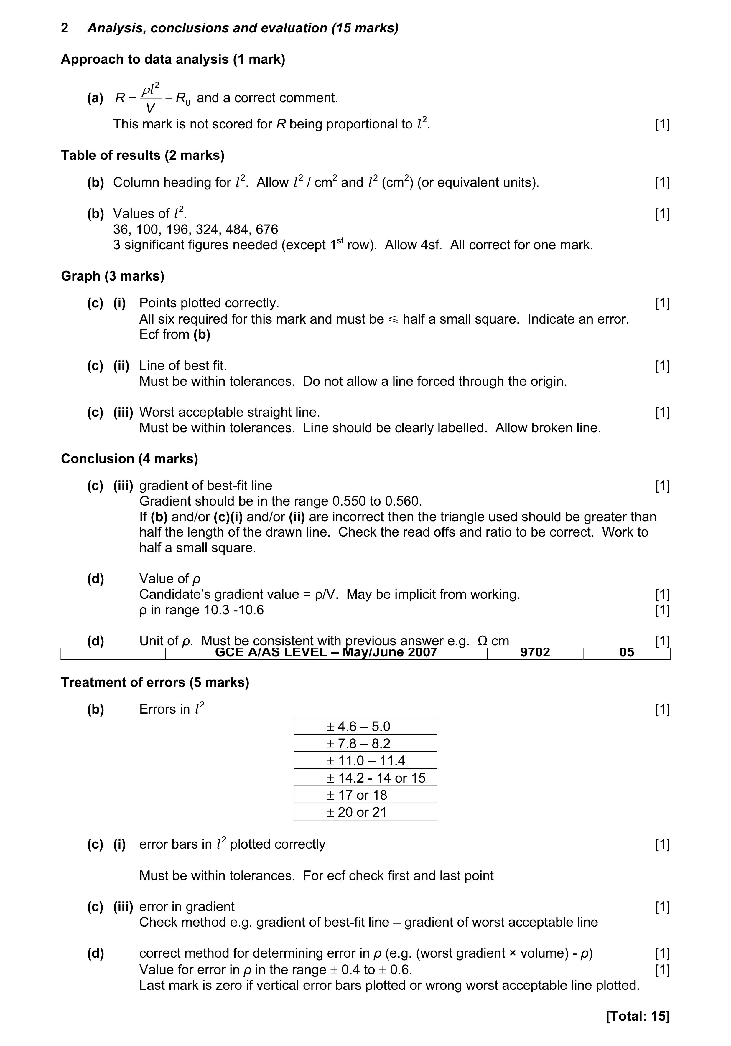
Mark scheme: 2 Analysis, conclusions and evaluation (15 marks) Approach to data analysis (1 mark) ρl 2 (a) R = + R 0 and a correct comment. V This mark is not scored for R being proportional to l 2. [1] Table of results (2 marks) (b) Column heading for l 2. Allow l 2 / cm2 and l 2 (cm2) (or equivalent units). [1] (b) Values of l 2. [1] 36, 100, 196, 324, 484, 676 3 significant figures needed (except 1st row). Allow 4sf. All correct for one mark. Graph (3 marks) (c) (i) Points plotted correctly. [1] All six required for this mark and must be Ğ half a small square. Indicate an error. Ecf from (b) (c) (ii) Line of best fit. [1] Must be within tolerances. Do not allow a line forced through the origin. (c) (iii) Worst acceptable straight line. [1] Must be within tolerances. Line should be clearly labelled. Allow broken line. Conclusion (4 marks) (c) (iii) gradient of best-fit line [1] Gradient should be in the range 0.550 to 0.560. If (b) and/or (c)(i) and/or (ii) are incorrect then the triangle used should be greater than half the length of the drawn line. Check the read offs and ratio to be correct. Work to half a small square. (d) Value of ρ Candidate’s gradient value = ρ/V. May be implicit from working. [1] ρ in range 10.3 -10.6 [1] (d) Unit of ρ. Must be consistent with previous answer e.g. Ω cm [1] GCE A/AS LEVEL – May/June 2007 9702 05 Treatment of errors (5 marks) (b) Errors in l 2 [1] ± 4.6 – 5.0 ± 7.8 – 8.2 ± 11.0 – 11.4 ± 14.2 - 14 or 15 ± 17 or 18 ± 20 or 21 (c) (i) error bars in l 2 plotted correctly [1] Must be within tolerances. For ecf check first and last point (c) (iii) error in gradient [1] Check method e.g. gradient of best-fit line – gradient of worst acceptable line (d) correct method for determining error in ρ (e.g. (worst gradient × volume) - ρ) [1] Value for error in ρ in the range ± 0.4 to ± 0.6. [1] Last mark is zero if vertical error bars plotted or wrong worst acceptable line plotted. [Total: 15]
This question in 9702/51 May/June 2007
Q2 · A student wishes to measure the resistivity of glass 9702/51 May/June 2008
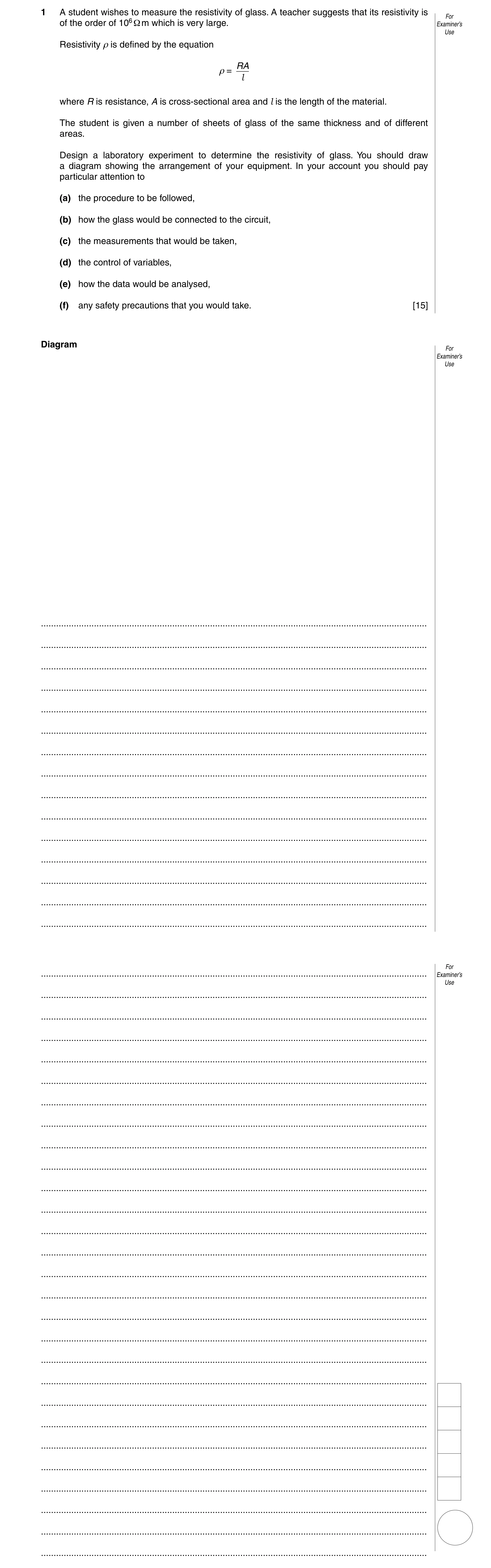
1 A student wishes to measure the resistivity of glass. A teacher suggests that its resistivity is For of the order of 106 Ω m which is very large. Examiner’s Use Resistivity ρ is defined by the equation RA ρ = l where R is resistance, A is cross-sectional area and l is the length of the material. The student is given a number of sheets of glass of the same thickness and of different areas. Design a laboratory experiment to determine the resistivity of glass. You should draw a diagram showing the arrangement of your equipment. In your account you should pay particular attention to (a) the procedure to be followed, (b) how the glass would be connected to the circuit, (c) the measurements that would be taken, (d) the control of variables, (e) how the data would be analysed, (f) any safety precautions that you would take. [15] Diagram For Examiner’s Use … … … … … … … … … … … … … … … For … Examiner’s Use … … … … … … … … … … … … … … … … … … … … … … … … … … …
15 marks
Mark scheme: 1 Planning (15 marks) Defining the problem (3 marks) P1 A is the independent variable or vary A. [1] P2 R is the dependent variable or determine R for different A. [1] P3 Keep the temperature (of glass) constant. Do not allow “controlled variable”. [1] Methods of data collection (5 marks) M1 Basic circuit diagram. [1] Ammeter and voltmeter with power supply, or ohmmeter without power supply, or bridge methods. M2 Correct orientation of glass between electrodes – largest cross-sectional area. [1] M3 A distance (thickness) measured using a micrometer/vernier scale/vernier callipers. [1] M4 Method of determining area perpendicular to current flow. [1] Distances measured and multiplied together. This mark may only be scored if it is clear that the correct dimensions are being used. M5 Method of determining resistance. [1] Ohmmeter. R = V/I justified. Description of balancing bridge with correct equation. Method of analysis (2 marks) A1 A2 R against 1/A ρ = gradient/l R against l /A ρ = gradient 1/A against R or 1/R against A ρ = 1/(gradient × l) l /A against R or l /R against A ρ = 1/gradient lg R against lg A ρ = 10l × y-intercept [2] Safety considerations (1 mark) S1 Relevant safety precaution related to: [1] EHT power supply (>100 V) – switch off before changing circuit/use of rubber gloves; or handling glass – wear (thick) gloves. Additional detail (4 marks) D1/2/3/4 Relevant points might include [4] Calculation of typical resistance of glass using value of resistivity given. Range of ammeter or ohmmeter with reasoning. Use of EHT or power supply >1000 V or microammeter/galvanometer. Take many readings of thickness and average. Good contact between circuit and glass e.g. metal plates, foil, conducting putty. Metal plates/foil/conducting putty to cover all of the cross-sectional area in use. Method of securing good contact between circuit and glass, e.g. g clamps, weights. Clean/dry the glass. [Total: 15] GCE A/AS LEVEL – May/June 2008 9702 05
This question in 9702/51 May/June 2008
Q3 · A student wishes to determine the resistivity of aluminium 9702/53 Oct/Nov 2010
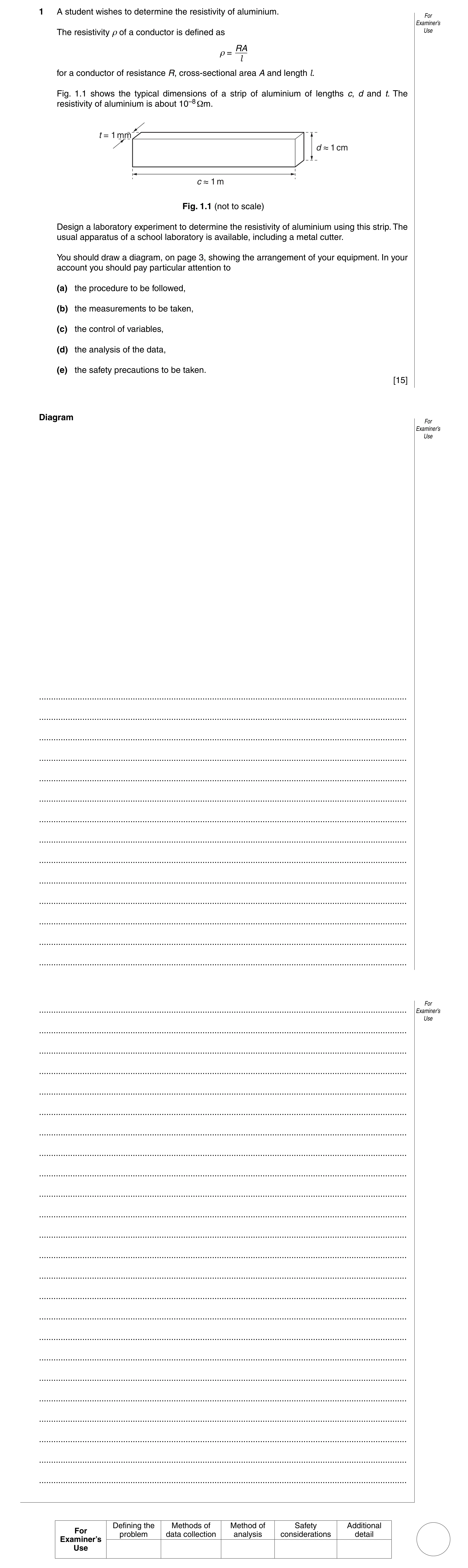
1 A student wishes to determine the resistivity of aluminium. For Examiner’s The resistivity ρ of a conductor is defined as Use RA ρ = l for a conductor of resistance R, cross-sectional area A and length l. Fig. 1.1 shows the typical dimensions of a strip of aluminium of lengths c, d and t. The resistivity of aluminium is about 10–8 Ωm. t = 1 mm d 1 cm c 1 m Fig. 1.1 (not to scale) Design a laboratory experiment to determine the resistivity of aluminium using this strip. The usual apparatus of a school laboratory is available, including a metal cutter. You should draw a diagram, on page 3, showing the arrangement of your equipment. In your account you should pay particular attention to (a) the procedure to be followed, (b) the measurements to be taken, (c) the control of variables, (d) the analysis of the data, (e) the safety precautions to be taken. [15] Diagram For Examiner’s Use … … … … … … … … … … … … … … For … Examiner’s Use … … … … … … … … … … … … … … … … … … … … … … … Defining the Methods of Method of Safety Additional For problem data collection analysis considerations detail Examiner’s Use
15 marks
Mark scheme: 1 Planning (15 marks) Defining the problem (3 marks) P1 c, d or A is the independent variable and R is the dependent variable or vary c, d or A and measure R. [1] P2 If c varied then (t and) d or A kept constant, if d varied then (t and) c or A kept constant, if A varied then c or d kept constant. [1] P3 Keep temperature constant. [1] Methods of data collection (5 marks) M1 Circuit diagram to measure resistance. [1] M2 Use micrometer screw gauge to measure d or t. (Allow digital or vernier callipers) [1] M3 Measure c with a ruler/metre rule. [1] M4 Method of making contact with the strip e.g. use electrodes of at least same dimension as c or d or t or conducting paint methods. Do not allow crocodile clips, unless it is clear that the whole area of the end of the strip is covered. [1] M5 Method to determine resistance. [1] Method of analysis (2 marks) A1 Plot a graph of R against c, 1/d or 1/A depending on orientation. Other alternatives possible, e.g. R against 1/c depending on orientation [1] A2 Must be consistent with A1: ρ = A × gradient or t × gradient/c [1] Other alternatives possible, e.g. ρ = d × gradient/t Safety considerations (1 mark) S1 Reference sharp edges or cutting metals, e.g. wear gloves. [1] Additional detail (4 marks) D1/2/3/4 Relevant points might include [4] 1. Insulate aluminium strip 2. Take many readings of t or d and average 3. Use a protective resistor/circuit designed to reduce current 4. Rearrange equation to determine graph using c, d and t or A 5. Determine typical resistance of aluminium strip 6. Likely meter range of ammeter/voltmeter/ohmmeter 7. Detail on cutting strip e.g. mark using set square Do not allow vague computer methods. [Total: 15] GCE A/AS LEVEL – October/November 2010 9702 53
This question in 9702/53 Oct/Nov 2010
Q4 · A student is investigating a non-inverting operational amplifier (op-amp) circuit 9702/53 May/June 2011
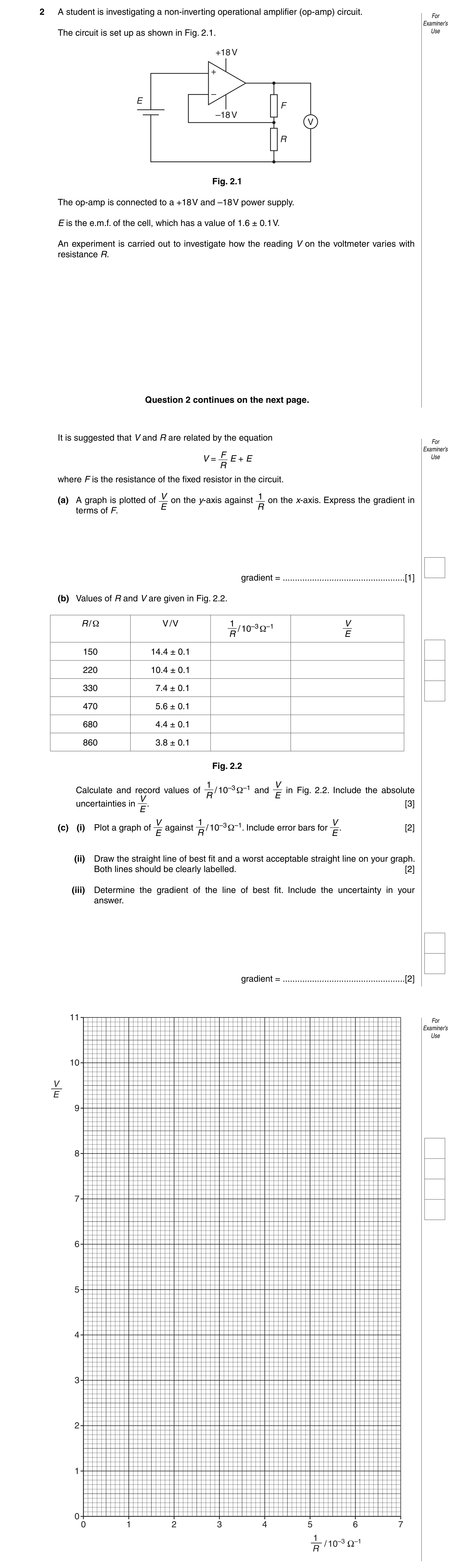
2 A student is investigating a non-inverting operational amplifier (op-amp) circuit. For Examiner’s The circuit is set up as shown in Fig. 2.1. Use +18 V + – E F –18 V V R Fig. 2.1 The op-amp is connected to a +18 V and –18 V power supply. E is the e.m.f. of the cell, which has a value of 1.6 ± 0.1 V. An experiment is carried out to investigate how the reading V on the voltmeter varies with resistance R. Question 2 continues on the next page. It is suggested that V and R are related by the equation For Examiner’s F Use V = E + E R where F is the resistance of the fixed resistor in the circuit. V 1(a) A graph is plotted of on the y-axis against on the x-axis. Express the gradient in E R terms of F. gradient = … [1] (b) Values of R and V are given in Fig. 2.2. R / Ω V / V 1 V / 10–3 Ω–1 R E 150 14.4 ± 0.1 220 10.4 ± 0.1 330 7.4 ± 0.1 470 5.6 ± 0.1 680 4.4 ± 0.1 860 3.8 ± 0.1 Fig. 2.2 1 V Calculate and record values of / 10–3 Ω–1 and in Fig. 2.2. Include the absolute R E V uncertainties in . [3] E V 1 V (c) (i) Plot a graph of against / 10–3 Ω–1. Include error bars for . [2] E R E (ii) Draw the straight line of best fit and a worst acceptable straight line on your graph. Both lines should be clearly labelled. [2] (iii) Determine the gradient of the line of best fit. Include the uncertainty in your answer. gradient = … [2] 11 For Examiner’s Use 10 V E 9 8 7 6 5 4 3 2 1 0 0 1 2 3 4 5 6 7 1 / 10–3 Ω–1 R
10 marks
Mark scheme: 2 Analysis, conclusions and evaluation (15 marks) Part Mark Expected Answer Additional Guidance (a) A1 F (b) T1 6.7 or 6.67 9.0 or 9.00 T1 for 1/R. T2 4.5 or 4.55 6.5 or 6.50 T2 for V/E. 3.0 or 3.03 4.6 or 4.63 Must be 2sf or 3sf; a mixture is allowed 2.1 or 2.13 3.5 or 3.50 1.5 or 1.47 2.8 or 2.75 1.2 or 1.16 2.4 or 2.38 U1 From ± 0.6 or ± 0.7, to ± 0.2 Allow more than one significant figure. (c) (i) G1 Six points plotted correctly Check second and fifth plots and other anomalous plots. Must be less than half a small square. Ecf allowed from table. U2 All error bars in V/E plotted correctly Half square or greater loses the mark. Ecf allowed from table. (ii) G2 Line of best fit If points are plotted correctly then lower end of line should pass between (0, 0.9) and (0, 1.1) and upper end of line should pass between (7, 9.3) and (7, 9.5). Allow ecf from points plotted incorrectly – examiner judgement. G3 Worst acceptable straight line. Line should be clearly labelled or dashed. Steepest or shallowest possible line Should pass from top of top error bar to that passes through all the error bars. bottom of bottom error bar or bottom of top error bar to top of bottom error bar. Mark scored only if error bars are plotted. (iii) C1 Gradient of best fit line The triangle used should be at least half the length of the drawn line. Check the read offs. Work to half a small square. Do not penalise POT. U3 Uncertainty in gradient Method of determining absolute uncertainty. Difference in worst gradient and gradient. (d) C2 (Gradient value) Ω Gradient must be used correctly. Expect about 1200 Ω Allow ecf from (c)(iii) but penalise POT. Do not penalise sf or rounding errors. U4 Determines uncertainty in F Allow ecf from POT. (e) (i) C3 Determines V/E correctly. Answer should be approximately 11; F from (d) must be used. F + 1 R U5 Determines absolute uncertainty Should be approximately 15% of RF/R1 (about 1.5). Several possible methods. (ii) C4 In the range 17.2 to 18.0 given to 2 or Allow 17 or 18 to 2sf. 3sf Must be (e)(i) × 1.6 [Total: 15] GCE AS/A LEVEL – May/June 2011 9702 53 Uncertainties in Question 2 (c) (iii) Gradient [U3] Uncertainty = gradient of line of best fit – gradient of worst acceptable line Uncertainty = ½ (steepest worst line gradient – shallowest worst line gradient) (d) [U4] Uncertainty = uncertainty in gradient (e) [U5] Uncertainty = worst V/E – V/E Note worst V/E is calculated either by max V/min E or by min V/max E Or max gradient of WAL/114 or min gradient of WAL/126 ∆m F Uncertainty = 0.05 + × [Allow V/E instead of F/R] m R ∆F F Uncertainty = 0.05 + × [Allow V/E instead of F/R] F R 6 ∆m F Uncertainty = + × [Allow V/E instead of F/R] 120 m R 6 ∆F F Uncertainty = + × [Allow V/E instead of F/R] 120 F R
This question in 9702/53 May/June 2011
Q5 · A student is investigating how the resistance R of nichrome in the form of a wire varies… 9702/53 Oct/Nov 2013
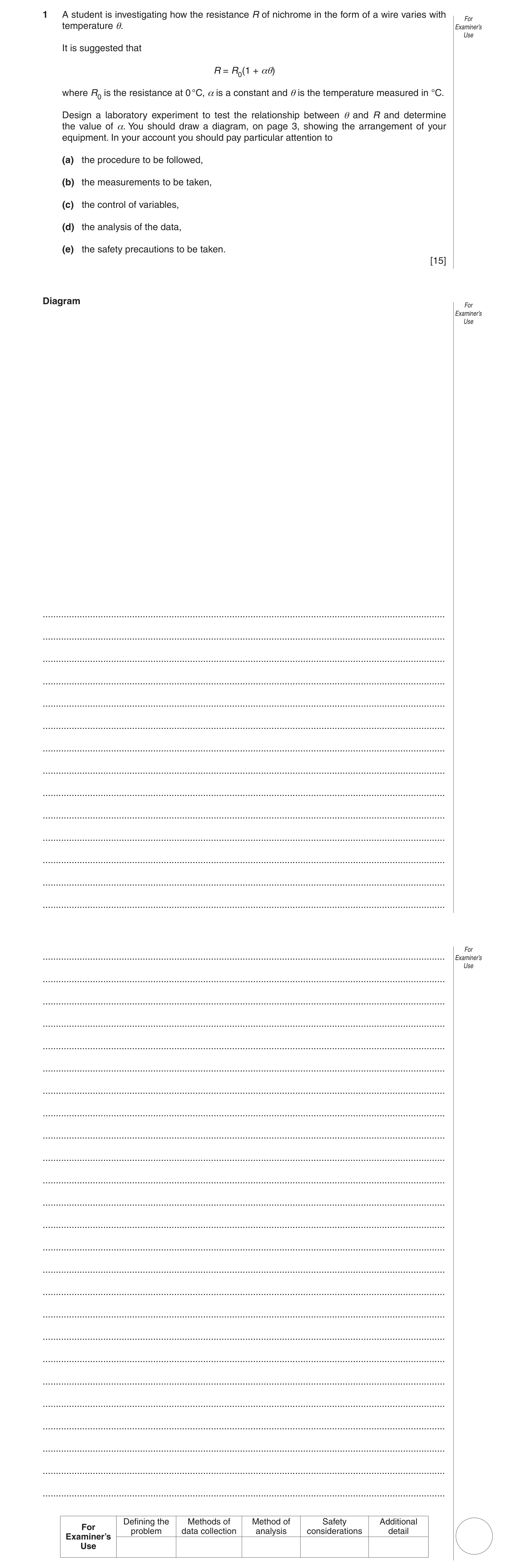
1 A student is investigating how the resistance R of nichrome in the form of a wire varies with For temperature θ. Examiner’s Use It is suggested that R = R0(1 + aθ) where R0 is the resistance at 0 °C, a is a constant and θ is the temperature measured in °C. Design a laboratory experiment to test the relationship between θ and R and determine the value of a. You should draw a diagram, on page 3, showing the arrangement of your equipment. In your account you should pay particular attention to (a) the procedure to be followed, (b) the measurements to be taken, (c) the control of variables, (d) the analysis of the data, (e) the safety precautions to be taken. [15] Diagram For Examiner’s Use … … … … … … … … … … … … … … For … Examiner’s Use … … … … … … … … … … … … … … … … … … … … … … … … Defining the Methods of Method of Safety Additional For problem data collection analysis considerations detail Examiner’s Use
15 marks
Mark scheme: 1 Planning (15 marks) Defining the problem (3 marks) P θ is the independent variable or vary θ. [1] P R is the dependent variable or measure R. [1] P Keep length of wire constant. [1] Methods of data collection (5 marks) M Labelled diagram of apparatus: wire in oil/water bath or oven or beaker with water and source of heat. [1] M Circuit diagram to measure resistance. [1] M Use thermometer to measure the temperature of wire/water/oven. (Could be on diagram if labelled.) [1] M Method to determine resistance from circuit, e.g. read off ohmmeter/R = V/I [1] M Method to determine R0 e.g. use ice-water mixture. Do not allow ice (allow ice at 0 °C or melting ice). [1] Method of analysis (2 marks) Do NOT allow log-log graphs. A R against θ R/R0 against θ θ against R [1] A α = gradient/R0 α = gradient α = 1/ (R0 × gradient) [1] α = – 1/y–intercept Safety considerations (1 mark) S Reasoned method to prevent injury from hot water/hot wire e.g. gloves (to prevent injury) from hot water/wire; goggles to prevent splashes from hot water; do not touch hot wire/beaker. [1] Additional detail (4 marks) D Relevant points might include [4] 1 Use insulated wire 2 Use long/thin wire to increase resistance 3 Stir liquid 4 Wait for temperature to stabilise 5 Relationship is valid if straight line, provided plotted graph is correct 6 Relationship is valid if straight line not passing through origin, provided plotted graph is correct (any quoted expression must be correct, e.g. y-intercept = R0) 7 Use small current to minimise heating effect Do not allow vague computer methods. [Total 15] GCE AS/A LEVEL – October/November 2013 9702 53
This question in 9702/53 Oct/Nov 2013
Q6 · A student is investigating the performance of a motor vehicle 9702/51 May/June 2015
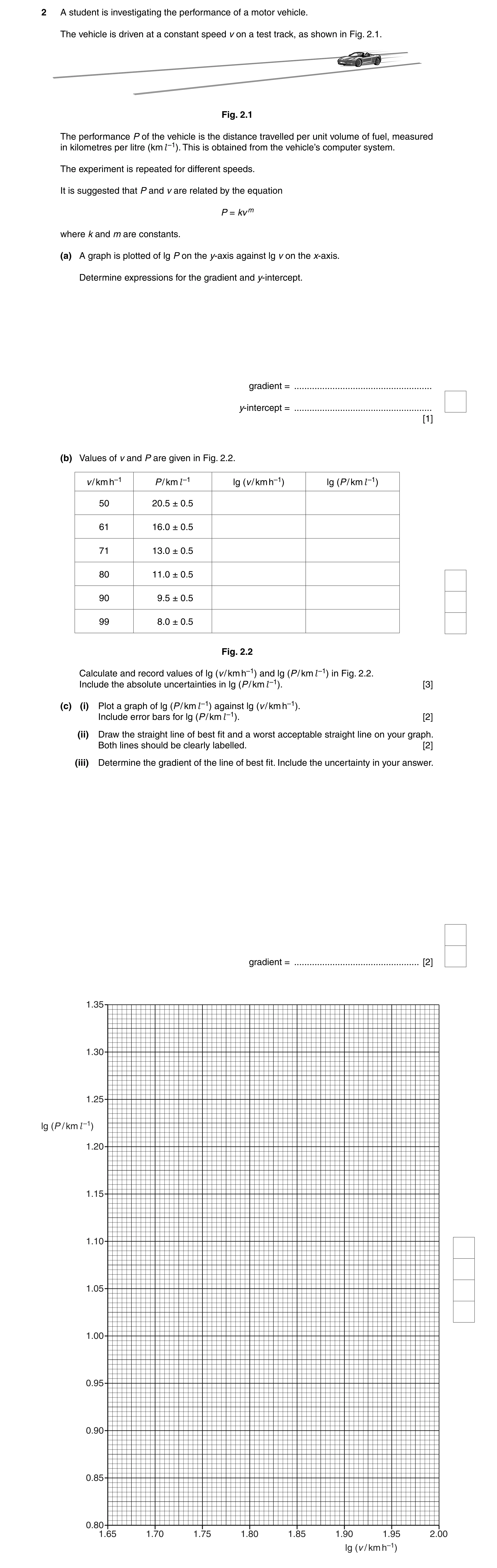
2 A student is investigating the performance of a motor vehicle. The vehicle is driven at a constant speed v on a test track, as shown in Fig. 2.1. Fig. 2.1 The performance P of the vehicle is the distance travelled per unit volume of fuel, measured in kilometres per litre (km l –1). This is obtained from the vehicle’s computer system. The experiment is repeated for different speeds. It is suggested that P and v are related by the equation P = kv m where k and m are constants. (a) A graph is plotted of lg P on the y-axis against lg v on the x-axis. Determine expressions for the gradient and y-intercept. gradient = … y-intercept = … [1] (b) Values of v and P are given in Fig. 2.2. v / km h–1 P / km l –1 lg (v / km h–1) lg (P / km l –1) 50 20.5 ± 0.5 61 16.0 ± 0.5 71 13.0 ± 0.5 80 11.0 ± 0.5 90 9.5 ± 0.5 99 8.0 ± 0.5 Fig. 2.2 Calculate and record values of lg (v / km h–1) and lg (P / km l –1) in Fig. 2.2. Include the absolute uncertainties in lg (P / km l –1). [3] (c) (i) Plot a graph of lg (P / km l –1) against lg (v / km h–1). Include error bars for lg (P / km l –1). [2] (ii) Draw the straight line of best fit and a worst acceptable straight line on your graph. Both lines should be clearly labelled. [2] (iii) Determine the gradient of the line of best fit. Include the uncertainty in your answer. gradient = … [2] 1.35 1.30 1.25 lg (P / km l –1) 1.20 1.15 1.10 1.05 1.00 0.95 0.90 0.85 0.80 1.65 1.70 1.75 1.80 1.85 1.90 1.95 2.00 lg (v / km h–1)
10 marks
Mark scheme: 2 Analysis, conclusions and evaluation (15 marks) Mark Expected Answer Additional Guidance (a) A1 gradient = m y-intercept = lg k (b) T1 Allow a mixture of significant figures. T2 1.70 or 1.699 1.312 or 1.3118 T1 (first column) and T2 (second column) must be values in table. 1.79 or 1.785 1.204 or 1.2041 1.85 or 1.851 1.114 or 1.1139 1.90 or 1.903 1.041 or 1.0414 1.95 or 1.954 0.98 or 0.978 2.00 or 1.996 0.90 or 0.903 U1 From ±0.01 to ±0.03 Allow more than one significant figure. (c) (i) G1 Six points plotted correctly Must be within half a small square. Do not allow “blobs”. Ecf allowed from table. U2 Error bars in lg P plotted correctly All error bars to be plotted. Must be accurate to less than half a small square. (ii) G2 Line of best fit Upper end of line must pass between (1.75, 1.24) and (1.75, 1.255) and lower end of line must pass between (2.00, 0.900) and (2.00, 0.915). G3 Worst acceptable straight line. Line should be clearly labelled or dashed. Steepest or shallowest possible Examiner judgement on worst acceptable line that passes through all the line. Lines must cross. Mark scored only if error bars. error bars are plotted. (iii) C1 Gradient of line of best fit Must be negative. The triangle used should be at least half the length of the drawn line. Check the read-offs. Work to half a small square. Do not penalise POT. (Should be about –1.35.) U3 Uncertainty in gradient Method of determining absolute uncertainty: difference in worst gradient and gradient. (iv) C2 y-intercept Check substitution into y = mx + c. Allow ecf from (c)(iii). (Should be about 4.) Do not allow read-off of false origin. U4 Uncertainty in y-intercept Uses worst gradient and point on worst acceptable line. Do not check calculation. Do not allow if false origin used. (d) (i) C3 k = 10y-intercept C4 m = gradient and given to 2 or 3 s.f. Must be negative. and in the range –1.30 to –1.44 Allow –1.3 or –1.4 (2 s.f.) (ii) U5 Percentage uncertainty in k Uncertainties in Question 2 (c) (iii) Gradient [U3] uncertainty = gradient of line of best fit – gradient of worst acceptable line uncertainty = ½ (steepest worst line gradient – shallowest worst line gradient) (iv) [U4] uncertainty = y-intercept of line of best fit – y-intercept of worst acceptable line uncertainty = ½ (steepest worst line y-intercept – shallowest worst line y-intercept) (d) (ii) [U5] max k = 10max y-intercept and min k = 10min y-intercept 1 (max k − min k ) max k − k k − min k 2 percentage uncertainty = × 100 = × 100 = × 100 k k k
This question in 9702/51 May/June 2015
Q7 · A student is investigating the performance of a motor vehicle 9702/53 May/June 2015
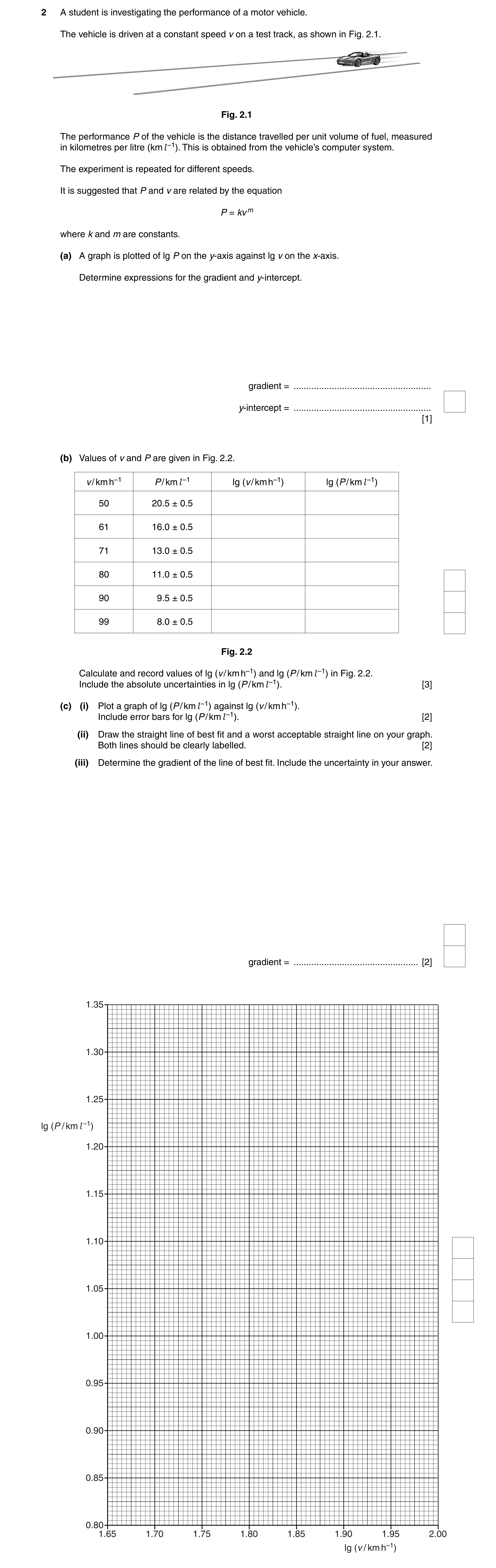
2 A student is investigating the performance of a motor vehicle. The vehicle is driven at a constant speed v on a test track, as shown in Fig. 2.1. Fig. 2.1 The performance P of the vehicle is the distance travelled per unit volume of fuel, measured in kilometres per litre (km l –1). This is obtained from the vehicle’s computer system. The experiment is repeated for different speeds. It is suggested that P and v are related by the equation P = kv m where k and m are constants. (a) A graph is plotted of lg P on the y-axis against lg v on the x-axis. Determine expressions for the gradient and y-intercept. gradient = … y-intercept = … [1] (b) Values of v and P are given in Fig. 2.2. v / km h–1 P / km l –1 lg (v / km h–1) lg (P / km l –1) 50 20.5 ± 0.5 61 16.0 ± 0.5 71 13.0 ± 0.5 80 11.0 ± 0.5 90 9.5 ± 0.5 99 8.0 ± 0.5 Fig. 2.2 Calculate and record values of lg (v / km h–1) and lg (P / km l –1) in Fig. 2.2. Include the absolute uncertainties in lg (P / km l –1). [3] (c) (i) Plot a graph of lg (P / km l –1) against lg (v / km h–1). Include error bars for lg (P / km l –1). [2] (ii) Draw the straight line of best fit and a worst acceptable straight line on your graph. Both lines should be clearly labelled. [2] (iii) Determine the gradient of the line of best fit. Include the uncertainty in your answer. gradient = … [2] 1.35 1.30 1.25 lg (P / km l –1) 1.20 1.15 1.10 1.05 1.00 0.95 0.90 0.85 0.80 1.65 1.70 1.75 1.80 1.85 1.90 1.95 2.00 lg (v / km h–1)
10 marks
Mark scheme: 2 Analysis, conclusions and evaluation (15 marks) Mark Expected Answer Additional Guidance (a) A1 gradient = m y-intercept = lg k (b) T1 Allow a mixture of significant figures. T2 1.70 or 1.699 1.312 or 1.3118 T1 (first column) and T2 (second column) must be values in table. 1.79 or 1.785 1.204 or 1.2041 1.85 or 1.851 1.114 or 1.1139 1.90 or 1.903 1.041 or 1.0414 1.95 or 1.954 0.98 or 0.978 2.00 or 1.996 0.90 or 0.903 U1 From ±0.01 to ±0.03 Allow more than one significant figure. (c) (i) G1 Six points plotted correctly Must be within half a small square. Do not allow “blobs”. Ecf allowed from table. U2 Error bars in lg P plotted correctly All error bars to be plotted. Must be accurate to less than half a small square. (ii) G2 Line of best fit Upper end of line must pass between (1.75, 1.24) and (1.75, 1.255) and lower end of line must pass between (2.00, 0.900) and (2.00, 0.915). G3 Worst acceptable straight line. Line should be clearly labelled or dashed. Steepest or shallowest possible Examiner judgement on worst acceptable line that passes through all the line. Lines must cross. Mark scored only if error bars. error bars are plotted. (iii) C1 Gradient of line of best fit Must be negative. The triangle used should be at least half the length of the drawn line. Check the read-offs. Work to half a small square. Do not penalise POT. (Should be about –1.35.) U3 Uncertainty in gradient Method of determining absolute uncertainty: difference in worst gradient and gradient. (iv) C2 y-intercept Check substitution into y = mx + c. Allow ecf from (c)(iii). (Should be about 4.) Do not allow read-off of false origin. U4 Uncertainty in y-intercept Uses worst gradient and point on worst acceptable line. Do not check calculation. Do not allow if false origin used. (d) (i) C3 k = 10y-intercept C4 m = gradient and given to 2 or 3 s.f. Must be negative. and in the range –1.30 to –1.44 Allow –1.3 or –1.4 (2 s.f.) (ii) U5 Percentage uncertainty in k Uncertainties in Question 2 (c) (iii) Gradient [U3] uncertainty = gradient of line of best fit – gradient of worst acceptable line uncertainty = ½ (steepest worst line gradient – shallowest worst line gradient) (iv) [U4] uncertainty = y-intercept of line of best fit – y-intercept of worst acceptable line uncertainty = ½ (steepest worst line y-intercept – shallowest worst line y-intercept) (d) (ii) [U5] max k = 10max y-intercept and min k = 10min y-intercept 1 (max k − min k ) max k − k k − min k 2 percentage uncertainty = × 100 = × 100 = × 100 k k k
This question in 9702/53 May/June 2015
Q8 · A student is investigating an electrical circuit containing a length of nichrome wire 9702/51 Oct/Nov 2015
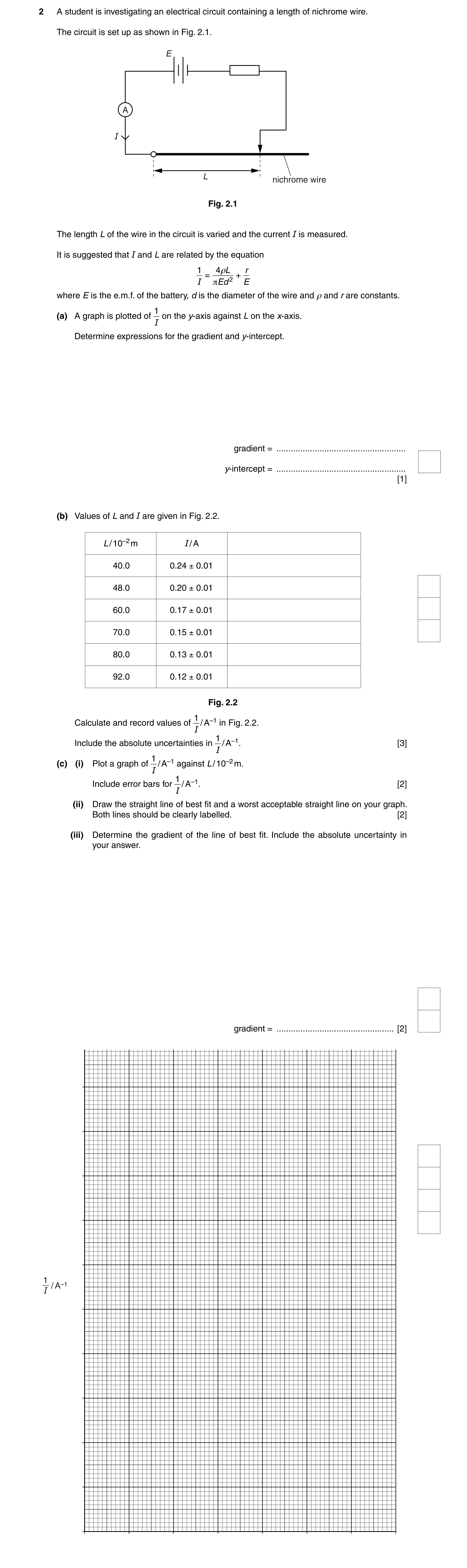
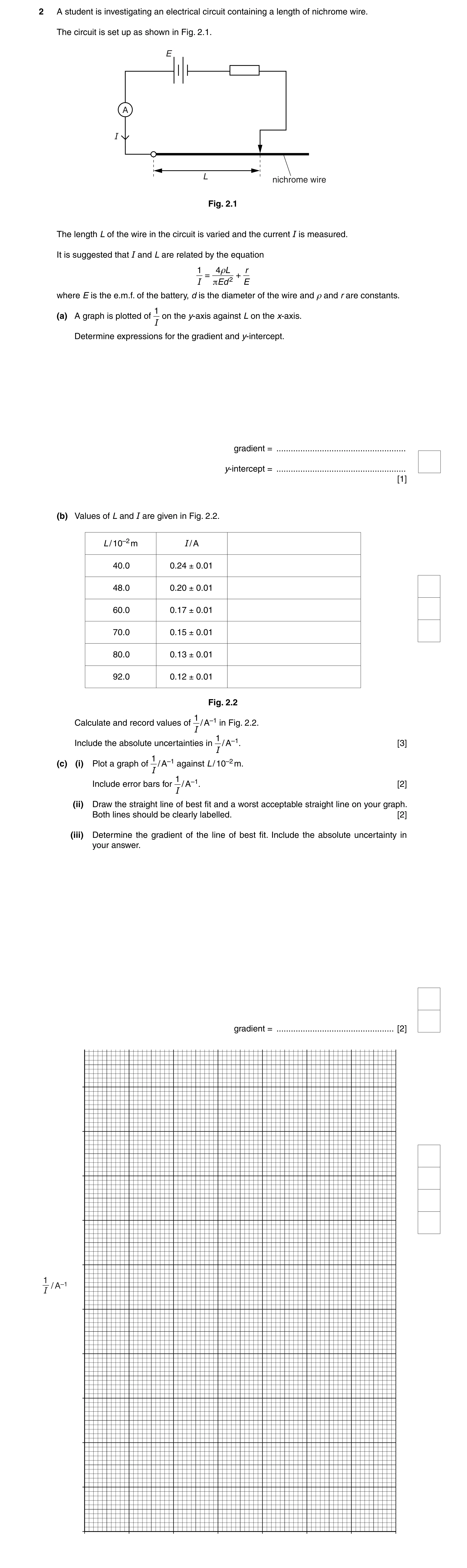
2 A student is investigating an electrical circuit containing a length of nichrome wire. The circuit is set up as shown in Fig. 2.1. E A I L nichrome wire Fig. 2.1 The length L of the wire in the circuit is varied and the current I is measured. It is suggested that I and L are related by the equation 1 4ρL r = + I πEd 2 E where E is the e.m.f. of the battery, d is the diameter of the wire and ρ and r are constants. 1 (a) A graph is plotted of on the y-axis against L on the x-axis. I Determine expressions for the gradient and y-intercept. gradient = … y-intercept = … [1] (b) Values of L and I are given in Fig. 2.2. L / 10–2 m I / A 40.0 0.24 ± 0.01 48.0 0.20 ± 0.01 60.0 0.17 ± 0.01 70.0 0.15 ± 0.01 80.0 0.13 ± 0.01 92.0 0.12 ± 0.01 Fig. 2.2 1 Calculate and record values of / A–1 in Fig. 2.2. I 1 Include the absolute uncertainties in / A–1. [3] I 1(c) (i) Plot a graph of / A–1 against L / 10–2 m. I 1 Include error bars for / A–1. [2] I (ii) Draw the straight line of best fit and a worst acceptable straight line on your graph. Both lines should be clearly labelled. [2] (iii) Determine the gradient of the line of best fit. Include the absolute uncertainty in your answer. gradient = … [2] 1 / $²I
10 marks
Mark scheme: 2 Analysis, conclusions and evaluation (15 marks) Mark Expected Answer Additional Guidance (a) A1 4 ρ gradient = 2 πEd r y-intercept = E (b) T1 1 1 1 1 / A–1 Allow (A–1) or . I I I A T2 Allow a mixture of significant figures. 4.2 or 4.17 Must be table values. 5.0 or 5.00 5.9 or 5.88 6.7 or 6.67 7.7 or 7.69 8.3 or 8.33 U1 ± 0.2 to ± 0.6 or ± 0.7 or ± 0.8 Allow more than one significant figure. (c) (i) G1 Six points plotted correctly Must be within half a small square. Do not allow “blobs”. ECF allowed from table. U2 Error bars in 1 / I plotted All error bars to be plotted. Must be accurate to correctly less than half a small square. Length of bar must be accurate to less than half a small square. Do not allow less than 0.05. (ii) G2 Line of best fit If points are plotted correctly then lower end of line should pass between (41, 4.5) and (44, 4.5) and upper end of line should pass between (83, 8.0) and (88, 8.0). Line should not go from bottom to top points. G3 Worst acceptable straight line. Line should be clearly labelled or dashed. Steepest or shallowest Examiner judgement on worst acceptable line. possible line that passes Lines must cross. Mark scored only if error bars through all the error bars. are plotted. (iii) C1 Gradient of line of best fit The triangle used should be at least half the length of the drawn line. Check the read-offs. Work to half a small square. Do not penalise POT. (Should be about 8.) U3 Absolute uncertainty in Method of determining absolute uncertainty: gradient difference in worst gradient and gradient. (iv) C2 y-intercept Check substitution into y = mx + c. Allow ECF from (c)(iii). (Should be about 0.7–1.5.) U4 Absolute uncertainty in y- Uses worst gradient and point on WAL. intercept Do not check calculation. (d) (i) C3 ρ = 2.415 × 10⁻⁷ × gradient Must use gradient. πEd 2 ρ = × gradient Must be in the range 4 1.80 × 10⁻⁶ to 2.10 × 10⁻⁶ and [2 × 10⁻⁶ Ω m = 2 × 10⁻⁴ Ω cm = 2 × 10⁻³ Ω mm] given to 2 or 3 s.f. C4 r = E × y-intercept Must include units for ρ and r. = 3.2 × y-intercept Allow V A–1 or kg m2 A–2 s–3 for Ω. and Ω m and Ω given (ii) U5 Percentage uncertainty in ρ Must be greater than 9.6%. Uncertainties in Question 2 (c) (iii) Gradient [U3] uncertainty = gradient of line of best fit – gradient of worst acceptable line uncertainty = ½ (steepest worst line gradient – shallowest worst line gradient) (iv) [U4] uncertainty = y-intercept of line of best fit – y-intercept of worst acceptable line uncertainty = ½ (steepest worst line y-intercept – shallowest worst line y-intercept) (d) (ii) [U5] ∆m 0.1 0.01 percentage uncertainty = + + 2 × × 100 m 3.2 0.31 ∆m = × 100 + 3.125 + 2 × 3.226 m − 3 2 π × 3.3 × (0.32 × 10 ) max. p = × max. gradient 4 − 3 2 π × 3.1 × (0.30 × 10 ) min. p = × min. gradient 4
This question in 9702/51 Oct/Nov 2015
Q9 · A student is investigating an electrical circuit containing a length of nichrome wire 9702/52 Oct/Nov 2015
2 A student is investigating an electrical circuit containing a length of nichrome wire. The circuit is set up as shown in Fig. 2.1. E A I L nichrome wire Fig. 2.1 The length L of the wire in the circuit is varied and the current I is measured. It is suggested that I and L are related by the equation 1 4ρL r = + I πEd 2 E where E is the e.m.f. of the battery, d is the diameter of the wire and ρ and r are constants. 1 (a) A graph is plotted of on the y-axis against L on the x-axis. I Determine expressions for the gradient and y-intercept. gradient = … y-intercept = … [1] (b) Values of L and I are given in Fig. 2.2. L / 10–2 m I / A 40.0 0.24 ± 0.01 48.0 0.20 ± 0.01 60.0 0.17 ± 0.01 70.0 0.15 ± 0.01 80.0 0.13 ± 0.01 92.0 0.12 ± 0.01 Fig. 2.2 1 Calculate and record values of / A–1 in Fig. 2.2. I 1 Include the absolute uncertainties in / A–1. [3] I 1(c) (i) Plot a graph of / A–1 against L / 10–2 m. I 1 Include error bars for / A–1. [2] I (ii) Draw the straight line of best fit and a worst acceptable straight line on your graph. Both lines should be clearly labelled. [2] (iii) Determine the gradient of the line of best fit. Include the absolute uncertainty in your answer. gradient = … [2] 1 / $²I
10 marks
Mark scheme: 2 Analysis, conclusions and evaluation (15 marks) Mark Expected Answer Additional Guidance (a) A1 4 ρ gradient = 2 πEd r y-intercept = E (b) T1 1 1 1 1 / A–1 Allow (A–1) or . I I I A T2 Allow a mixture of significant figures. 4.2 or 4.17 Must be table values. 5.0 or 5.00 5.9 or 5.88 6.7 or 6.67 7.7 or 7.69 8.3 or 8.33 U1 ± 0.2 to ± 0.6 or ± 0.7 or ± 0.8 Allow more than one significant figure. (c) (i) G1 Six points plotted correctly Must be within half a small square. Do not allow “blobs”. ECF allowed from table. U2 Error bars in 1 / I plotted All error bars to be plotted. Must be accurate to correctly less than half a small square. Length of bar must be accurate to less than half a small square. Do not allow less than 0.05. (ii) G2 Line of best fit If points are plotted correctly then lower end of line should pass between (41, 4.5) and (44, 4.5) and upper end of line should pass between (83, 8.0) and (88, 8.0). Line should not go from bottom to top points. G3 Worst acceptable straight line. Line should be clearly labelled or dashed. Steepest or shallowest Examiner judgement on worst acceptable line. possible line that passes Lines must cross. Mark scored only if error bars through all the error bars. are plotted. (iii) C1 Gradient of line of best fit The triangle used should be at least half the length of the drawn line. Check the read-offs. Work to half a small square. Do not penalise POT. (Should be about 8.) U3 Absolute uncertainty in Method of determining absolute uncertainty: gradient difference in worst gradient and gradient. (iv) C2 y-intercept Check substitution into y = mx + c. Allow ECF from (c)(iii). (Should be about 0.7–1.5.) U4 Absolute uncertainty in y- Uses worst gradient and point on WAL. intercept Do not check calculation. (d) (i) C3 ρ = 2.415 × 10⁻⁷ × gradient Must use gradient. πEd 2 ρ = × gradient Must be in the range 4 1.80 × 10⁻⁶ to 2.10 × 10⁻⁶ and [2 × 10⁻⁶ Ω m = 2 × 10⁻⁴ Ω cm = 2 × 10⁻³ Ω mm] given to 2 or 3 s.f. C4 r = E × y-intercept Must include units for ρ and r. = 3.2 × y-intercept Allow V A–1 or kg m2 A–2 s–3 for Ω. and Ω m and Ω given (ii) U5 Percentage uncertainty in ρ Must be greater than 9.6%. Uncertainties in Question 2 (c) (iii) Gradient [U3] uncertainty = gradient of line of best fit – gradient of worst acceptable line uncertainty = ½ (steepest worst line gradient – shallowest worst line gradient) (iv) [U4] uncertainty = y-intercept of line of best fit – y-intercept of worst acceptable line uncertainty = ½ (steepest worst line y-intercept – shallowest worst line y-intercept) (d) (ii) [U5] ∆m 0.1 0.01 percentage uncertainty = + + 2 × × 100 m 3.2 0.31 ∆m = × 100 + 3.125 + 2 × 3.226 m − 3 2 π × 3.3 × (0.32 × 10 ) max. p = × max. gradient 4 − 3 2 π × 3.1 × (0.30 × 10 ) min. p = × min. gradient 4
This question in 9702/52 Oct/Nov 2015
Q10 · A student is interested in ‘bungee jumping’, where a person attached to an elastic cord… 9702/52 Feb/March 2016
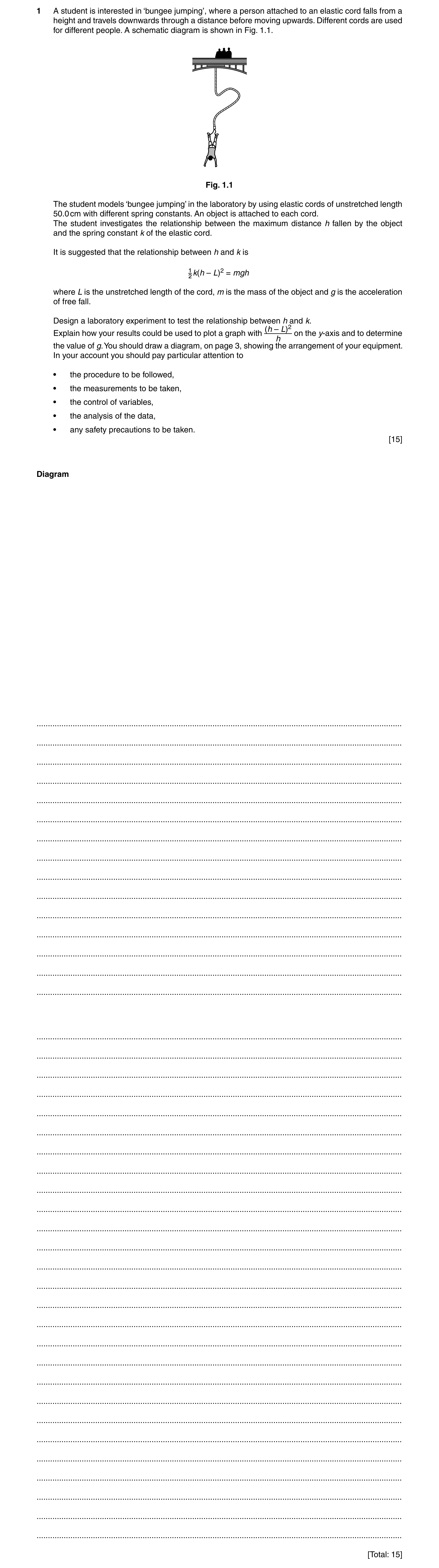
1 A student is interested in ‘bungee jumping’, where a person attached to an elastic cord falls from a height and travels downwards through a distance before moving upwards. Different cords are used for different people. A schematic diagram is shown in Fig. 1.1. Fig. 1.1 The student models ‘bungee jumping’ in the laboratory by using elastic cords of unstretched length 50.0 cm with different spring constants. An object is attached to each cord. The student investigates the relationship between the maximum distance h fallen by the object and the spring constant k of the elastic cord. It is suggested that the relationship between h and k is k(h – L)2 = mgh where L is the unstretched length of the cord, m is the mass of the object and g is the acceleration of free fall. Design a laboratory experiment to test the relationship between h and k. (h – L)2 Explain how your results could be used to plot a graph with on the y-axis and to determine h the value of g. You should draw a diagram, on page 3, showing the arrangement of your equipment. In your account you should pay particular attention to • the procedure to be followed, • the measurements to be taken, • the control of variables, • the analysis of the data, • any safety precautions to be taken. [15] Diagram … … … … … … … … … … … … … … … … … … … … … … … … … … … … … … … … … … … … … … … … … … [Total: 15]
15 marks
Mark scheme: 1 Planning (15 marks) Defining the problem (2 marks) P k is the independent variable and h is the dependent variable, or vary k, measure h. [1] P Keep mass of object constant. [1] Methods of data collection (4 marks) M Labelled diagram (minimum two labels) showing object (mass) attached to cord and other end of cord fixed (e.g. stand and clamp or hook) and rule(r) drawn vertically next to cord. [1] M Method of measuring mass e.g. balance / scales. [1] M k = (weight or force) / extension or mg / extension; allow graphical methods. Allow any subject e.g. mg = k × extension. [1] M Use of rule to measure h or maximum distance / length (fallen by the object). Allow clear indication on diagram (i.e. dotted lines) linking distance h to rule. Do not credit length of cord. [1] Method of analysis (3 marks) ( h − L ) 2 Plot a graph of against 1 / k [Allow 2 / k or 2m / k or m / k] [1] h g = gradient / 2m [gradient / m or gradient or gradient / 2] [1] Relationship is valid if the graph is a straight line passing through the origin. [1] Additional detail (6 marks) D Relevant points [6] 1 Keep starting point constant/drop object from same position / use of electromagnet to drop object / ensure mass is dropped from fixed point / check object falls vertically 2 Rule(r) fixed e.g. retort stand 3 Method to determine extension, e.g. measure length of stretched cord and subtract original length / 50.0 cm. [Accept from a diagram] 4 Safety precaution linked to prevention of mass / cord hitting a person – use safety screen / goggles; sand tray to catch falling object if cord breaks 5 Trial experiment to locate approximate point of h / to prevent object hitting surface 6 Detailed use of video camera with slow motion or frame by frame playback / motion sensor clearly explained 7 Cord obeys Hooke’s law or must not exceed elastic limit 8 Use set square to ensure ruler is vertical 9 For each cord, repeat experiment determine average h Do not allow vague computer methods. [Total: 15 marks]
This question in 9702/52 Feb/March 2016
Q11 · A student is investigating the resistance of a light-dependent resistor (LDR) separated… 9702/51 Oct/Nov 2017
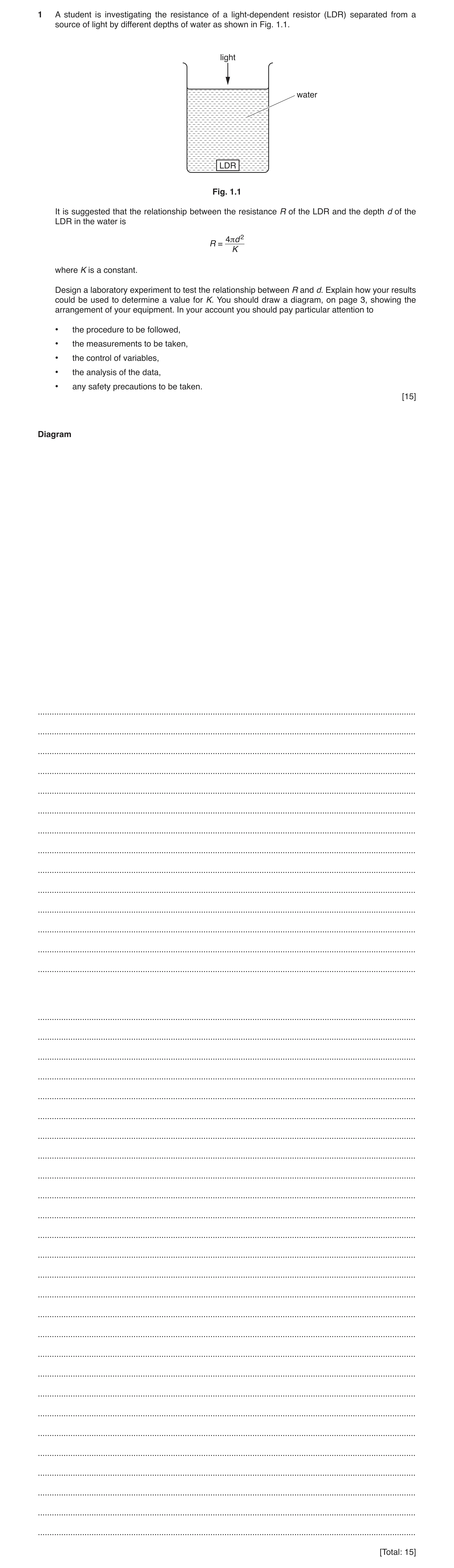
1 A student is investigating the resistance of a light-dependent resistor (LDR) separated from a source of light by different depths of water as shown in Fig. 1.1. light water LDR Fig. 1.1 It is suggested that the relationship between the resistance R of the LDR and the depth d of the LDR in the water is 4πd 2 R = K where K is a constant. Design a laboratory experiment to test the relationship between R and d. Explain how your results could be used to determine a value for K. You should draw a diagram, on page 3, showing the arrangement of your equipment. In your account you should pay particular attention to • the procedure to be followed, • the measurements to be taken, • the control of variables, • the analysis of the data, • any safety precautions to be taken. [15] Diagram … … … … … … … … … … … … … … … … … … … … … … … … … … … … … … … … … … … … … … … … … [Total: 15]
15 marks
Mark scheme: 1 Defining the problem d is the independent variable and R is the dependent variable or vary d and measure R 1 keep intensity/power of light source constant 1 Methods of data collection labelled diagram showing a light source fixed above container of water with the labelled LDR positioned in the beaker 1 correct circuit diagram to measure R, e.g. V and I methods or ohmmeter 1 method to determine R, e.g. = R p.d. across LDR current or read off ohmmeter 1 method to determine d, e.g. use a ruler or drawn labelled vertical ruler adjacent to container with d indicated 1 Method of analysis plots a graph of R against d2 1 relationship valid if a straight line produced passing through the origin 1 π = K 4 gradient 1 Question Answer Marks 1 Additional detail including safety considerations Max. 6 D1 dark glasses to prevent damage to eyes due to light source or do not look directly at light source or do not touch hot lamp/use gloves to position hot lamp/heat-proof gloves to position lamp D2 dark room or shielding LDR (so as to avoid light from other sources) D3 use high intensity lamp or collimated beam or laser D4 method described to check that current in light source is constant, e.g. use an ammeter and variable resistor / variable power supply D5 keep position of light source constant or distance between light source and LDR constant D6 light source is placed close to water surface to increase intensity/reduce reflections or light source is placed further away to make it more directional D7 use tall container to give a wide range of d or R or to reduce uncertainties or use a wide container to reduce reflections D8 method to position ruler vertically to measure d described e.g. use a set square/spirit level D9 use of horizontal fiducial mark from ruler to meniscus or middle of LDR, e.g. pin or d = reading on rule at surface – reading at top of LDR D10 ensure that the electrical connections/wire to the LDR are waterproof
This question in 9702/51 Oct/Nov 2017
Q12 · A student is investigating the resistance of a light-dependent resistor (LDR) separated… 9702/53 Oct/Nov 2017
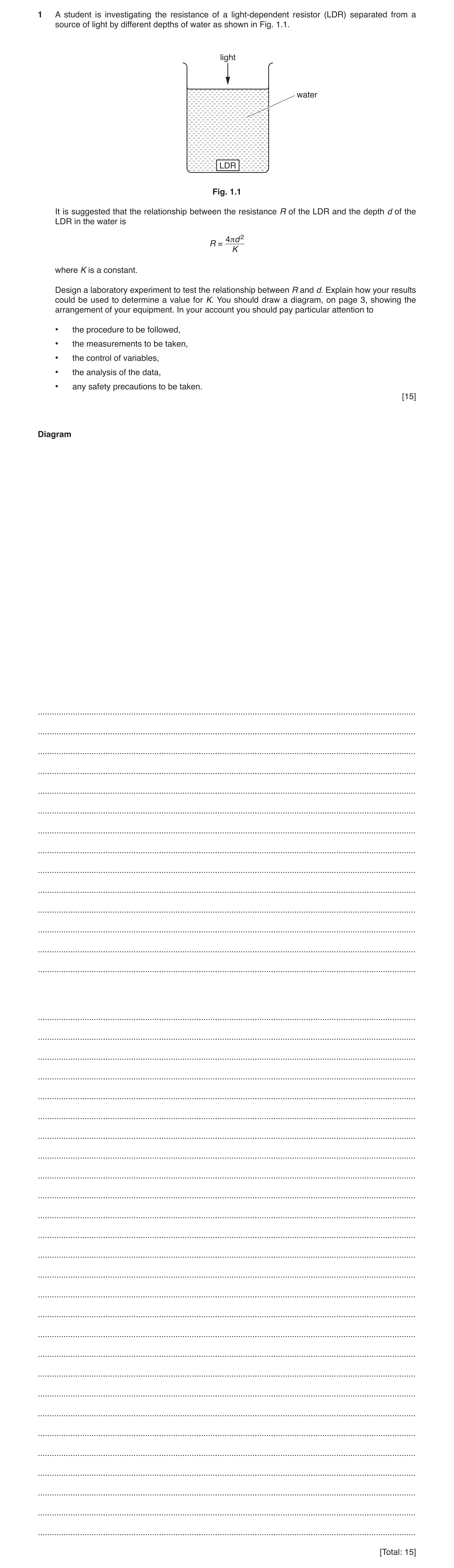
1 A student is investigating the resistance of a light-dependent resistor (LDR) separated from a source of light by different depths of water as shown in Fig. 1.1. light water LDR Fig. 1.1 It is suggested that the relationship between the resistance R of the LDR and the depth d of the LDR in the water is 4πd 2 R = K where K is a constant. Design a laboratory experiment to test the relationship between R and d. Explain how your results could be used to determine a value for K. You should draw a diagram, on page 3, showing the arrangement of your equipment. In your account you should pay particular attention to • the procedure to be followed, • the measurements to be taken, • the control of variables, • the analysis of the data, • any safety precautions to be taken. [15] Diagram … … … … … … … … … … … … … … … … … … … … … … … … … … … … … … … … … … … … … … … … … [Total: 15]
15 marks
Mark scheme: 1 Defining the problem d is the independent variable and R is the dependent variable or vary d and measure R 1 keep intensity/power of light source constant 1 Methods of data collection labelled diagram showing a light source fixed above container of water with the labelled LDR positioned in the beaker 1 correct circuit diagram to measure R, e.g. V and I methods or ohmmeter 1 method to determine R, e.g. = R p.d. across LDR current or read off ohmmeter 1 method to determine d, e.g. use a ruler or drawn labelled vertical ruler adjacent to container with d indicated 1 Method of analysis plots a graph of R against d2 1 relationship valid if a straight line produced passing through the origin 1 π = K 4 gradient 1 Question Answer Marks 1 Additional detail including safety considerations Max. 6 D1 dark glasses to prevent damage to eyes due to light source or do not look directly at light source or do not touch hot lamp/use gloves to position hot lamp/heat-proof gloves to position lamp D2 dark room or shielding LDR (so as to avoid light from other sources) D3 use high intensity lamp or collimated beam or laser D4 method described to check that current in light source is constant, e.g. use an ammeter and variable resistor / variable power supply D5 keep position of light source constant or distance between light source and LDR constant D6 light source is placed close to water surface to increase intensity/reduce reflections or light source is placed further away to make it more directional D7 use tall container to give a wide range of d or R or to reduce uncertainties or use a wide container to reduce reflections D8 method to position ruler vertically to measure d described e.g. use a set square/spirit level D9 use of horizontal fiducial mark from ruler to meniscus or middle of LDR, e.g. pin or d = reading on rule at surface – reading at top of LDR D10 ensure that the electrical connections/wire to the LDR are waterproof
This question in 9702/53 Oct/Nov 2017
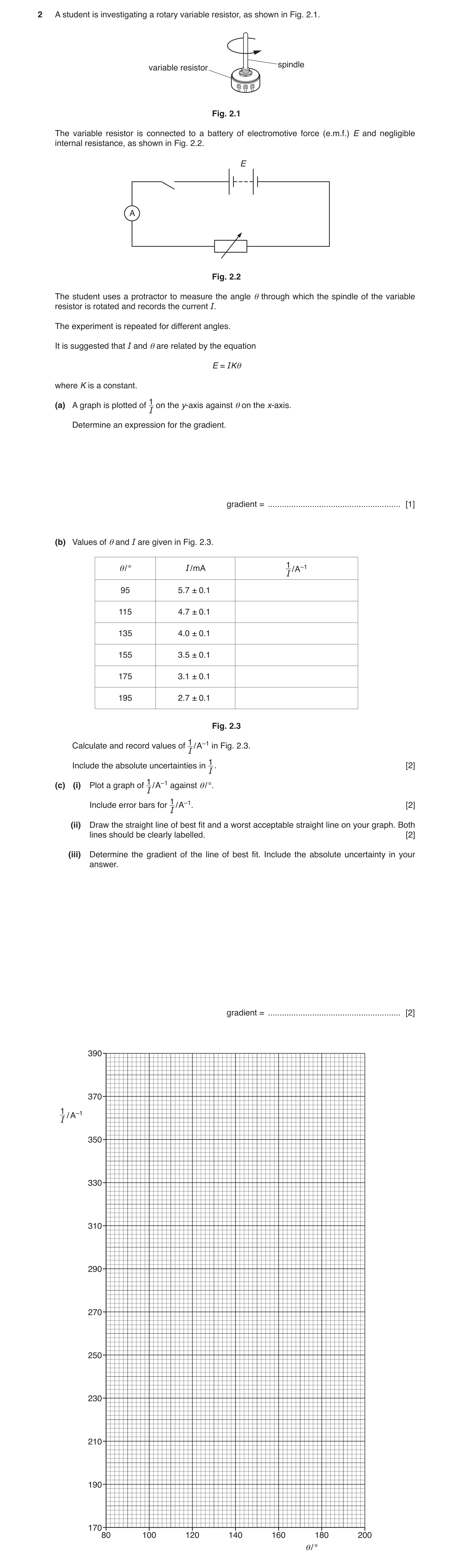
Q13 · A student is investigating a rotary variable resistor, as shown in Fig 9702/51 May/June 2019
2 A student is investigating a rotary variable resistor, as shown in Fig. 2.1. spindle variable resistor Fig. 2.1 The variable resistor is connected to a battery of electromotive force (e.m.f.) E and negligible internal resistance, as shown in Fig. 2.2. E A Fig. 2.2 The student uses a protractor to measure the angle θ through which the spindle of the variable resistor is rotated and records the current I. The experiment is repeated for different angles. It is suggested that I and θ are related by the equation E = IKθ where K is a constant. 1 on the y-axis against θ on the x-axis. (a) A graph is plotted of I Determine an expression for the gradient. gradient = … [1] (b) Values of θ and I are given in Fig. 2.3. 1 θ/ ° I / mA / A–1 I 95 5.7 ± 0.1 115 4.7 ± 0.1 135 4.0 ± 0.1 155 3.5 ± 0.1 175 3.1 ± 0.1 195 2.7 ± 0.1 Fig. 2.3 1 Calculate and record values of / A–1 in Fig. 2.3. I 1 Include the absolute uncertainties in . [2] I 1(c) (i) Plot a graph of / A–1 against θ/ °. I 1 Include error bars for / A–1. [2] I (ii) Draw the straight line of best fit and a worst acceptable straight line on your graph. Both lines should be clearly labelled. [2] (iii) Determine the gradient of the line of best fit. Include the absolute uncertainty in your answer. gradient = … [2]
9 marks
Mark scheme: 2(a) gradient = K E 2(b) 1 I / A–1 180 or 175 210 or 213 250 290 or 286 320 or 323 370 1 uncertainties in 1 I from ±3 or ±4 to ±10–15 1 2(c)(i) Six points plotted correctly. Must be accurate to the nearest half small square. Diameter of points must be less than half a small square. 1 Error bars in 1 I plotted correctly. All error bars to be plotted. Length of bar must be accurate to less than half a small square and symmetrical. 1 Question Answer Marks 2(c)(ii) Line of best fit drawn. Do not allow line from top point to bottom point. If points are plotted correctly then lower end of line should pass between (122, 230) and (126, 230) and upper end of line should pass between (186, 350) and (190, 350). 1 Worst acceptable line drawn (steepest or shallowest possible line that passes through all the error bars). All error bars must be plotted. 1 2(c)(iii) Gradient determined with clear substitution of points from the line into ∆y/∆x. Distance between points must be at least half the length of the drawn line. 1 uncertainty = gradient of line of best fit – gradient of worst acceptable line or uncertainty = ½ (steepest worst line gradient – shallowest worst line gradient) 1 2(d) 9.4 ± 0.2 (V) 1 2(e)(i) K determined from gradient and given to 2 or 3 significant figures. K = E × gradient = 9.4 × (c)(iii). 1 K determined from gradient with correct unit (Ω / °). 1 2(e)(ii) gradient % uncertainty in 100 gradient E K E ∆ ∆ = + × 1 Question Answer Marks 2(f) θ calculated. Correct substitution of numbers required. 9.4 0.01 E K θ = = × (e)(i) I or 1 1 gradient 0.01 θ = = × ×(c)(iii) I 1 Absolute uncertainty in θ. Correct substitution of numbers required. Use of ∆I not required but allow if included by the candidate. Using E and K: θ θ ∆ ∆ ∆ = + + × uncertainty in E K E K I I 0.2 uncertainty in 9.4 100 θ θ = + × (e)(ii) max min max min 0.01 min 0.01 max E E K K θ θ = = × × or Using gradient: θ θ ∆ ∆ = + × gradient uncertainty in gradient I I 1 1 max min 0.01 mingradient 0.01 maxgradient θ θ = = × × or 1
This question in 9702/51 May/June 2019
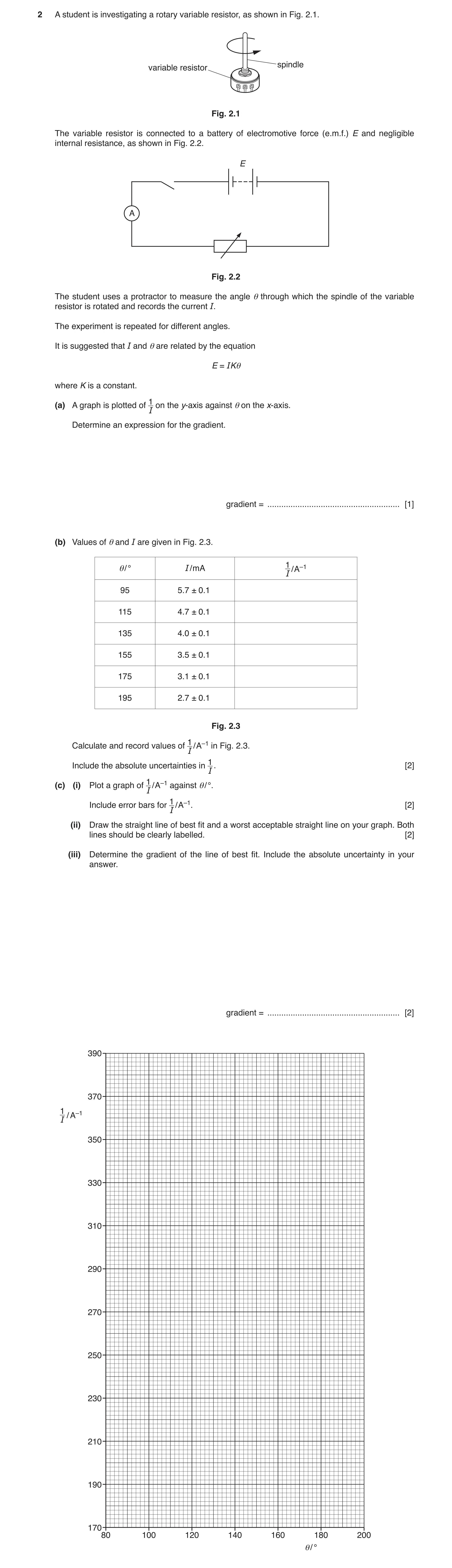
Q14 · A student is investigating a rotary variable resistor, as shown in Fig 9702/53 May/June 2019
2 A student is investigating a rotary variable resistor, as shown in Fig. 2.1. spindle variable resistor Fig. 2.1 The variable resistor is connected to a battery of electromotive force (e.m.f.) E and negligible internal resistance, as shown in Fig. 2.2. E A Fig. 2.2 The student uses a protractor to measure the angle θ through which the spindle of the variable resistor is rotated and records the current I. The experiment is repeated for different angles. It is suggested that I and θ are related by the equation E = IKθ where K is a constant. 1 on the y-axis against θ on the x-axis. (a) A graph is plotted of I Determine an expression for the gradient. gradient = … [1] (b) Values of θ and I are given in Fig. 2.3. 1 θ/ ° I / mA / A–1 I 95 5.7 ± 0.1 115 4.7 ± 0.1 135 4.0 ± 0.1 155 3.5 ± 0.1 175 3.1 ± 0.1 195 2.7 ± 0.1 Fig. 2.3 1 Calculate and record values of / A–1 in Fig. 2.3. I 1 Include the absolute uncertainties in . [2] I 1(c) (i) Plot a graph of / A–1 against θ/ °. I 1 Include error bars for / A–1. [2] I (ii) Draw the straight line of best fit and a worst acceptable straight line on your graph. Both lines should be clearly labelled. [2] (iii) Determine the gradient of the line of best fit. Include the absolute uncertainty in your answer. gradient = … [2]
9 marks
Mark scheme: 2(a) gradient = K E 2(b) 1 I / A–1 180 or 175 210 or 213 250 290 or 286 320 or 323 370 1 uncertainties in 1 I from ±3 or ±4 to ±10–15 1 2(c)(i) Six points plotted correctly. Must be accurate to the nearest half small square. Diameter of points must be less than half a small square. 1 Error bars in 1 I plotted correctly. All error bars to be plotted. Length of bar must be accurate to less than half a small square and symmetrical. 1 Question Answer Marks 2(c)(ii) Line of best fit drawn. Do not allow line from top point to bottom point. If points are plotted correctly then lower end of line should pass between (122, 230) and (126, 230) and upper end of line should pass between (186, 350) and (190, 350). 1 Worst acceptable line drawn (steepest or shallowest possible line that passes through all the error bars). All error bars must be plotted. 1 2(c)(iii) Gradient determined with clear substitution of points from the line into ∆y/∆x. Distance between points must be at least half the length of the drawn line. 1 uncertainty = gradient of line of best fit – gradient of worst acceptable line or uncertainty = ½ (steepest worst line gradient – shallowest worst line gradient) 1 2(d) 9.4 ± 0.2 (V) 1 2(e)(i) K determined from gradient and given to 2 or 3 significant figures. K = E × gradient = 9.4 × (c)(iii). 1 K determined from gradient with correct unit (Ω / °). 1 2(e)(ii) gradient % uncertainty in 100 gradient E K E ∆ ∆ = + × 1 Question Answer Marks 2(f) θ calculated. Correct substitution of numbers required. 9.4 0.01 E K θ = = × (e)(i) I or 1 1 gradient 0.01 θ = = × × (c)(iii) I 1 Absolute uncertainty in θ. Correct substitution of numbers required. Use of ∆I not required but allow if included by the candidate. Using E and K: θ θ ∆ ∆ ∆ = + + × uncertainty in E K E K I I 0.2 uncertainty in 9.4 100 θ θ = + × (e)(ii) max min max min 0.01 min 0.01 max E E K K θ θ = = × × or Using gradient: θ θ ∆ ∆ = + × gradient uncertainty in gradient I I 1 1 max min 0.01 mingradient 0.01 max gradient θ θ = = × × or 1
This question in 9702/53 May/June 2019
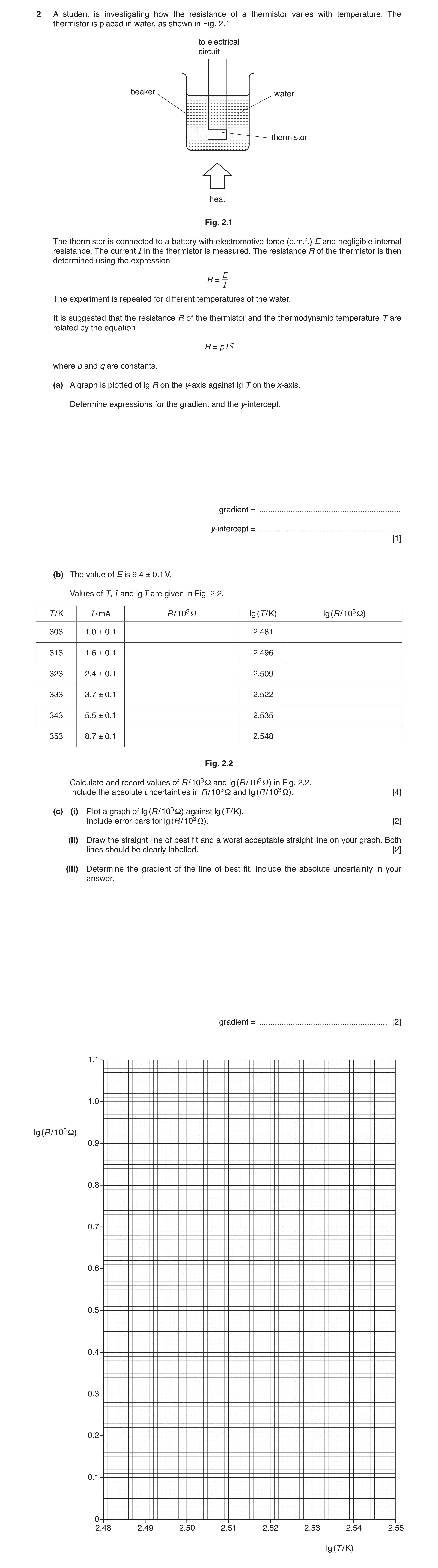
Q15 · A student is investigating how the resistance of a thermistor varies with temperature 9702/52 Oct/Nov 2019
2 A student is investigating how the resistance of a thermistor varies with temperature. The thermistor is placed in water, as shown in Fig. 2.1. to electrical circuit beaker water thermistor heat Fig. 2.1 The thermistor is connected to a battery with electromotive force (e.m.f.) E and negligible internal resistance. The current I in the thermistor is measured. The resistance R of the thermistor is then determined using the expression E R = . I The experiment is repeated for different temperatures of the water. It is suggested that the resistance R of the thermistor and the thermodynamic temperature T are related by the equation R = pT q where p and q are constants. (a) A graph is plotted of lg R on the y-axis against lg T on the x-axis. Determine expressions for the gradient and the y-intercept. gradient = … y-intercept = … [1] (b) The value of E is 9.4 ± 0.1 V. Values of T, I and lg T are given in Fig. 2.2. T / K I / mA R / 103 Ω lg (T / K) lg (R / 103 Ω) 303 1.0 ± 0.1 2.481 313 1.6 ± 0.1 2.496 323 2.4 ± 0.1 2.509 333 3.7 ± 0.1 2.522 343 5.5 ± 0.1 2.535 353 8.7 ± 0.1 2.548 Fig. 2.2 Calculate and record values of R / 103 Ω and lg (R / 103 Ω) in Fig. 2.2. Include the absolute uncertainties in R / 103 Ω and lg (R / 103 Ω). [4] (c) (i) Plot a graph of lg (R / 103 Ω) against lg (T / K). Include error bars for lg (R / 103 Ω). [2] (ii) Draw the straight line of best fit and a worst acceptable straight line on your graph. Both lines should be clearly labelled. [2] (iii) Determine the gradient of the line of best fit. Include the absolute uncertainty in your answer. gradient = … [2]
11 marks
Mark scheme: 2(a) and y-intercept = lg p 2(b) R / 103 Ω lg (R / 103 Ω) 9.4 or 9.40 0.97 or 0.973 5.9 or 5.88 0.77 or 0.771 or 0.769 3.9 or 3.92 0.59 or 0.591 or 0.593 2.5 or 2.54 0.40 or 0.398 or 0.405 1.7 or 1.71 0.23 or 0.230 or 0.233 1.1 or 1.08 0.04 or 0.041 or 0.033 Values of R as above. 1 Values of lg R as above. 1 Uncertainties in R from (±0.9 to ±1.2) to (±0.02 to ±0.03) and row 2 between ±0.40 and ±0.50 and row 4 between ±0.09 and ±0.10. 1 Uncertainties in lg R consistent with uncertainties in R e.g. from ±0.05 to ±0.01. 1 2(c)(i) Six points plotted correctly. Must be accurate to the nearest half a small square. Diameter of points must be less than half a small square. 1 Error bars in lg R plotted correctly. All error bars must be plotted. Length of bar must be accurate to less than half a small square and symmetrical. 1 Question Answer Marks 2(c)(ii) Line of best fit drawn. Upper end of line should pass between (2.500, 0.70) and (2.502, 0.70) and lower end of line should pass between (2.528, 0.30) and (2.532, 0.30). Do not accept line from first to last point. 1 Worst acceptable line drawn (steepest or shallowest possible line that passes through all the error bars). All error bars must be plotted. 1 2(c)(iii) Gradient determined with clear substitution of data points from the line of best fit into ∆y / ∆x. Distance between data points must be greater than half the length of the drawn line. Gradient must be negative. 1 uncertainty = gradient of line of best fit – gradient of worst acceptable line or uncertainty = ½ (steepest worst line gradient – shallowest worst line gradient) 1 2(c)(iv) y-intercept determined by substitution of correct point from the line of best fit into y = mx + c. 1 2(d) p determined from y-intercept. p (= 10y-intercept) = 10(c)(iv) 1 q = answer to (c)(iii) and given to 2 or 3 significant figures. 1 Question Answer Marks 2(e) T determined from (d) or (c)(iii) and (c)(iv) with correct substitution shown. 15 q q R T p p = = or − − = = lg15 lg 1.176 lg lg p p T q q − − = = lg15 -intercept 1.176 lg gradient y T (c)(iv) (c)(iii) − = 1.176 10 T (c)(iv) (c)(iii) 1
This question in 9702/52 Oct/Nov 2019
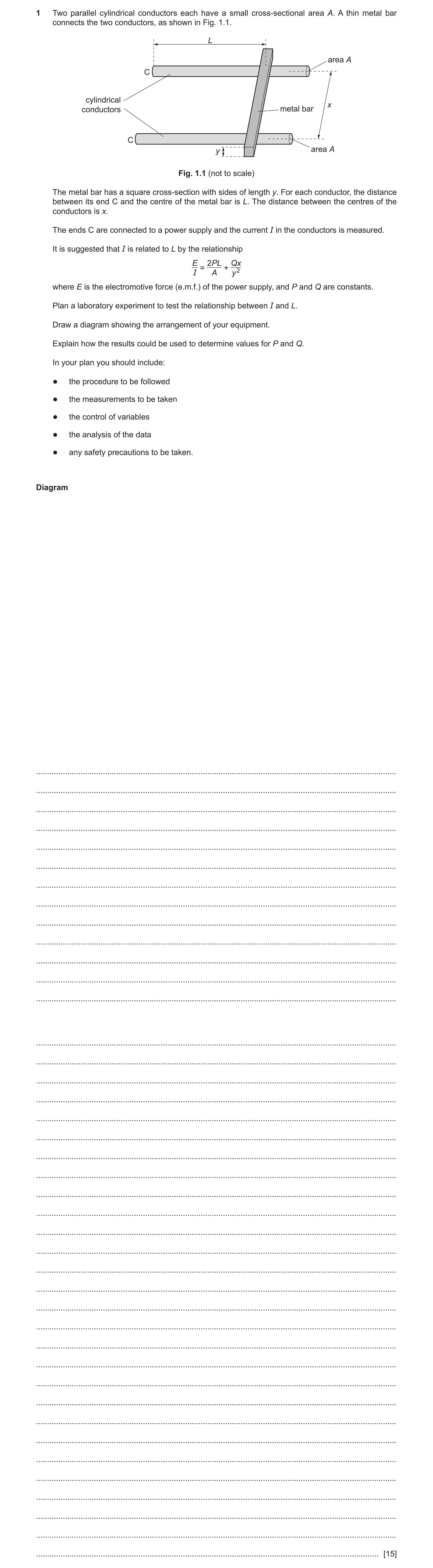
Q16 · Two parallel cylindrical conductors each have a small cross‑sectional area A 9702/52 May/June 2022
1 Two parallel cylindrical conductors each have a small cross‑sectional area A. A thin metal bar connects the two conductors, as shown in Fig. 1.1. L area A C cylindrical x conductors metal bar C y area A Fig. 1.1 (not to scale) The metal bar has a square cross‑section with sides of length y. For each conductor, the distance between its end C and the centre of the metal bar is L. The distance between the centres of the conductors is x. The ends C are connected to a power supply and the current I in the conductors is measured. It is suggested that I is related to L by the relationship E 2PL Qx = + 2 I A y where E is the electromotive force (e.m.f.) of the power supply, and P and Q are constants. Plan a laboratory experiment to test the relationship between I and L. Draw a diagram showing the arrangement of your equipment. Explain how the results could be used to determine values for P and Q. In your plan you should include: ● the procedure to be followed ● the measurements to be taken ● the control of variables ● the analysis of the data ● any safety precautions to be taken. Diagram … … … … … … … … … … … … … … … … … … … … … … … … … … … … … … … … … … … … … … … … … [15]
15 marks
Mark scheme: 1 Defining the problem L is the independent variable and I is the dependent variable or vary L and measure I 1 keep E constant 1 Methods of data collection labelled diagram of workable experiment including: circuit diagram with power supply connected to ends C ammeter in series with power supply and conductors correct symbol for ammeter and power supply 1 circuit diagram with voltmeter correctly positioned to measure E across the power supply 1 use a rule(r) to measure L and x 1 use a micrometer/calipers to measure y 1 Question Answer Marks 1 Method of analysis plot a graph of 1 I against L or equivalent (e.g. L against 1 I ) (Do not accept log graphs.) 1 gradient 2 AE P (for L against 1 I : 2 gradient AE P ) 1 2 -intercept y Ey Q x (for L against 1 I : 2 -intercept 2 y Py Q Ax or 2 -intercept gradient y Ey Q x ) 1 Question Answer Marks 1 Additional detail including safety considerations 6 D1 do not touch/use (heat resistant) gloves to avoid hot conductors/metal bar or use a protective resistor/small e.m.f. to reduce the current or switch off when not in use/when moving bar D2 keep A and y constant D3 keep x constant D4 use of micrometer/calipers to measure diameter of conductor and A = d2 / 4. D5 repeat measurements of diameter along conductors/different (perpendicular) directions/different points and average or repeat measurements of y in different (perpendicular) directions/different points/along bar and average D6 method to ensure that L is the same for each conductor, e.g. check both lengths D7 method to determine L e.g. measure to edge and add y / 2 or method to determine x e.g. measure between the conductors and add diameter D8 method to keep x constant with reason, e.g. adhesive/plasticine/blocks (one either side of each conductor) to prevent cylindrical conductors from moving D9 method of ensuring good electrical contact, e.g. clean metal bar/cylindrical conductors or use of solder or crocodile clips to connect circuit to the conductors D10 relationship valid if a straight line is produced (not passing through the origin)
This question in 9702/52 May/June 2022
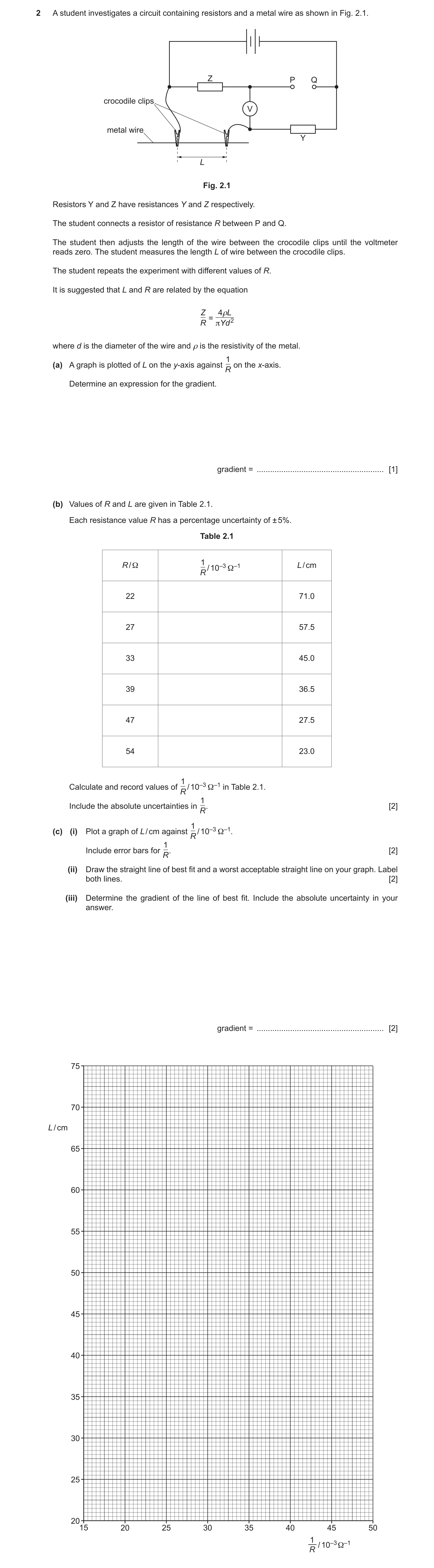
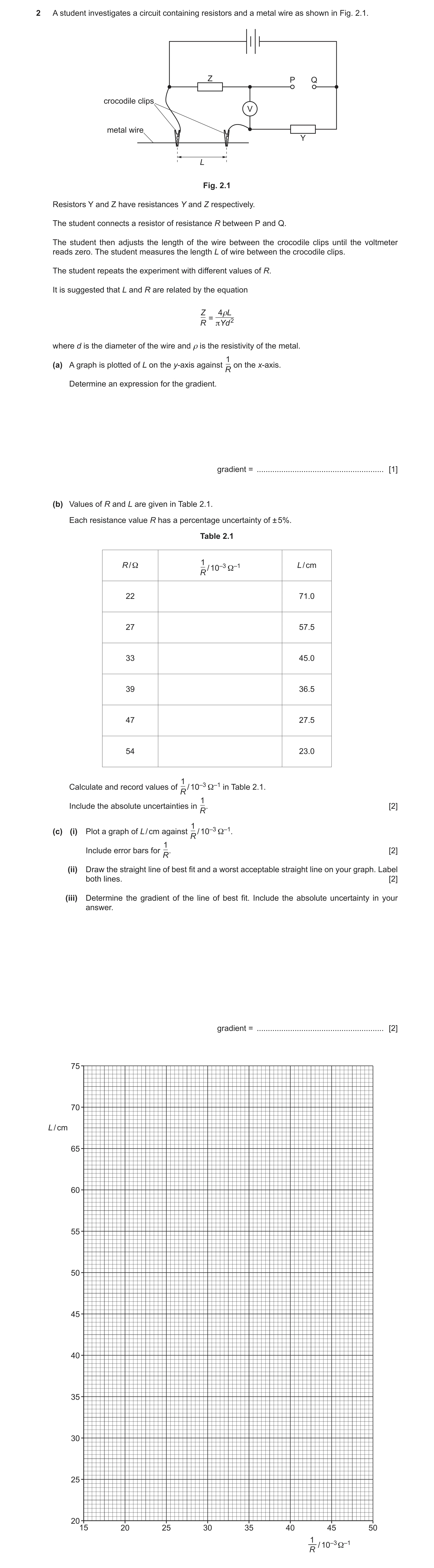
Q17 · A student investigates a circuit containing resistors and a metal wire as shown in Fig 9702/51 Oct/Nov 2022
2 A student investigates a circuit containing resistors and a metal wire as shown in Fig. 2.1. Z P Q crocodile clips V metal wire Y L Fig. 2.1 Resistors Y and Z have resistances Y and Z respectively. The student connects a resistor of resistance R between P and Q. The student then adjusts the length of the wire between the crocodile clips until the voltmeter reads zero. The student measures the length L of wire between the crocodile clips. The student repeats the experiment with different values of R. It is suggested that L and R are related by the equation Z 4ρL = R πYd 2 where d is the diameter of the wire and ρ is the resistivity of the metal. 1 (a) A graph is plotted of L on the y-axis against on the x-axis. R Determine an expression for the gradient. gradient = … [1] (b) Values of R and L are given in Table 2.1. Each resistance value R has a percentage uncertainty of ± 5%. Table 2.1 1 R / Ω / 10–3 Ω–1 L / cm R 22 71.0 27 57.5 33 45.0 39 36.5 47 27.5 54 23.0 1 Calculate and record values of / 10–3 Ω–1 in Table 2.1. R 1 Include the absolute uncertainties in R. [2] 1(c) (i) Plot a graph of L / cm against / 10–3 Ω–1. R 1 Include error bars for R. [2] (ii) Draw the straight line of best fit and a worst acceptable straight line on your graph. Label both lines. [2] (iii) Determine the gradient of the line of best fit. Include the absolute uncertainty in your answer. gradient = … [2]
9 marks
Mark scheme: 2(a) YZd 2 1 gradient = 4 2(b) 1 1 / 10–3 –1 R 45 or 45.5 37 or 37.0 30 or 30.3 26 or 25.6 21 or 21.3 19 or 18.5 1 1 Absolute uncertainties in from ± 2 to ± 0.9 or ± 1. R 2(c)(i) Six points from (b) plotted correctly. 1 Must be within half a small square. Diameter of points must be less than half a small square. 1 1 Error bars in plotted correctly. R All error bars to be plotted. Total length of bar must be accurate to less than half a small square and symmetrical. 2(c)(ii) Straight line of best fit drawn. 1 Points must be balanced. Do not accept line from top point to bottom point. Line must pass between (22.0, 30.0) and (23.0, 30.0) and (40.5, 65.0) and (42.0, 65.0). Worst acceptable line drawn (steepest or shallowest possible line that passes through all the error bars). 1 All error bars must be plotted. 2(c)(iii) Gradient determined with clear substitution of data points into y / x. 1 Distance between data points must be greater than half the length of the drawn line. Gradient of worst acceptable line determined with clear substitution of data points into y / x. 1 uncertainty = (gradient of line of best fit – gradient of worst acceptable line) or uncertainty = ½ (steepest worst line gradient – shallowest worst line gradient) 2(d) 0.261 ± 0.003 (mm) 1 2(e)(i) determined using gradient and given to two or three significant figures. 1 YZd 2 22 22 (d)2 = = 4 gradient 4 (c)(iii) determined using gradient and given with correct SI unit ( m) and correct power of ten 1 2(e)(ii) percentage uncertainty in : 1 2 d gradient percentage uncertainty = + + 0.05 + 0.05 100 d gradient or correct substitution for max/min methods (1.05 22 ) (1.05 22 ) ( d + d ) 2 max = 4 min gradient ( 0.95 22 ) ( 0.95 22 ) ( d −d ) 2 min = 4 max gradient 2(f) R determined to at least two significant figures from (c)(iii) or (d) and (e)(i) with correct substitution seen. 1 gradient R = 0.950 or YZd 2 22 22 (d) 2 R = = 4L 4 (e)(i) 0.950 Absolute uncertainty in R determined. 1 Method must be consistent with determination of R and correct substitution must be seen. for R determined using the gradient: gradient R = R gradient or for R determined using (d) and (e)(i): 2 d R = + + 0.05 + 0.05 R d or correct substitution for max/min methods: (1.05 22 ) (1.05 22 ) ( d + d ) 2 max R = 4 min 0.950 ( 0.95 22 ) ( 0.95 22 ) ( d −d ) 2 min R = 4 max 0.950
This question in 9702/51 Oct/Nov 2022
Q18 · A student investigates a circuit containing resistors and a metal wire as shown in Fig 9702/53 Oct/Nov 2022
2 A student investigates a circuit containing resistors and a metal wire as shown in Fig. 2.1. Z P Q crocodile clips V metal wire Y L Fig. 2.1 Resistors Y and Z have resistances Y and Z respectively. The student connects a resistor of resistance R between P and Q. The student then adjusts the length of the wire between the crocodile clips until the voltmeter reads zero. The student measures the length L of wire between the crocodile clips. The student repeats the experiment with different values of R. It is suggested that L and R are related by the equation Z 4ρL = R πYd 2 where d is the diameter of the wire and ρ is the resistivity of the metal. 1 (a) A graph is plotted of L on the y-axis against on the x-axis. R Determine an expression for the gradient. gradient = … [1] (b) Values of R and L are given in Table 2.1. Each resistance value R has a percentage uncertainty of ± 5%. Table 2.1 1 R / Ω / 10–3 Ω–1 L / cm R 22 71.0 27 57.5 33 45.0 39 36.5 47 27.5 54 23.0 1 Calculate and record values of / 10–3 Ω–1 in Table 2.1. R 1 Include the absolute uncertainties in R. [2] 1(c) (i) Plot a graph of L / cm against / 10–3 Ω–1. R 1 Include error bars for R. [2] (ii) Draw the straight line of best fit and a worst acceptable straight line on your graph. Label both lines. [2] (iii) Determine the gradient of the line of best fit. Include the absolute uncertainty in your answer. gradient = … [2]
9 marks
Mark scheme: 2(a) YZd 2 1 gradient = 4 2(b) 1 1 / 10–3 –1 R 45 or 45.5 37 or 37.0 30 or 30.3 26 or 25.6 21 or 21.3 19 or 18.5 1 1 Absolute uncertainties in from ± 2 to ± 0.9 or ± 1. R 2(c)(i) Six points from (b) plotted correctly. 1 Must be within half a small square. Diameter of points must be less than half a small square. 1 1 Error bars in plotted correctly. R All error bars to be plotted. Total length of bar must be accurate to less than half a small square and symmetrical. 2(c)(ii) Straight line of best fit drawn. 1 Points must be balanced. Do not accept line from top point to bottom point. Line must pass between (22.0, 30.0) and (23.0, 30.0) and (40.5, 65.0) and (42.0, 65.0). Worst acceptable line drawn (steepest or shallowest possible line that passes through all the error bars). 1 All error bars must be plotted. 2(c)(iii) Gradient determined with clear substitution of data points into y / x. 1 Distance between data points must be greater than half the length of the drawn line. Gradient of worst acceptable line determined with clear substitution of data points into y / x. 1 uncertainty = (gradient of line of best fit – gradient of worst acceptable line) or uncertainty = ½ (steepest worst line gradient – shallowest worst line gradient) 2(d) 0.261 ± 0.003 (mm) 1 2(e)(i) determined using gradient and given to two or three significant figures. 1 YZd 2 22 22 (d)2 = = 4 gradient 4 (c)(iii) determined using gradient and given with correct SI unit ( m) and correct power of ten 1 2(e)(ii) percentage uncertainty in : 1 2 d gradient percentage uncertainty = + + 0.05 + 0.05 100 d gradient or correct substitution for max/min methods (1.05 22 ) (1.05 22 ) ( d + d ) 2 max = 4 min gradient ( 0.95 22 ) ( 0.95 22 ) ( d −d ) 2 min = 4 max gradient 2(f) R determined to at least two significant figures from (c)(iii) or (d) and (e)(i) with correct substitution seen. 1 gradient R = 0.950 or YZd 2 22 22 (d) 2 R = = 4L 4 (e)(i) 0.950 Absolute uncertainty in R determined. 1 Method must be consistent with determination of R and correct substitution must be seen. for R determined using the gradient: gradient R = R gradient or for R determined using (d) and (e)(i): 2 d R = + + 0.05 + 0.05 R d or correct substitution for max/min methods: (1.05 22 ) (1.05 22 ) ( d + d ) 2 max R = 4 min 0.950 ( 0.95 22 ) ( 0.95 22 ) ( d −d ) 2 min R = 4 max 0.950
This question in 9702/53 Oct/Nov 2022
 10
10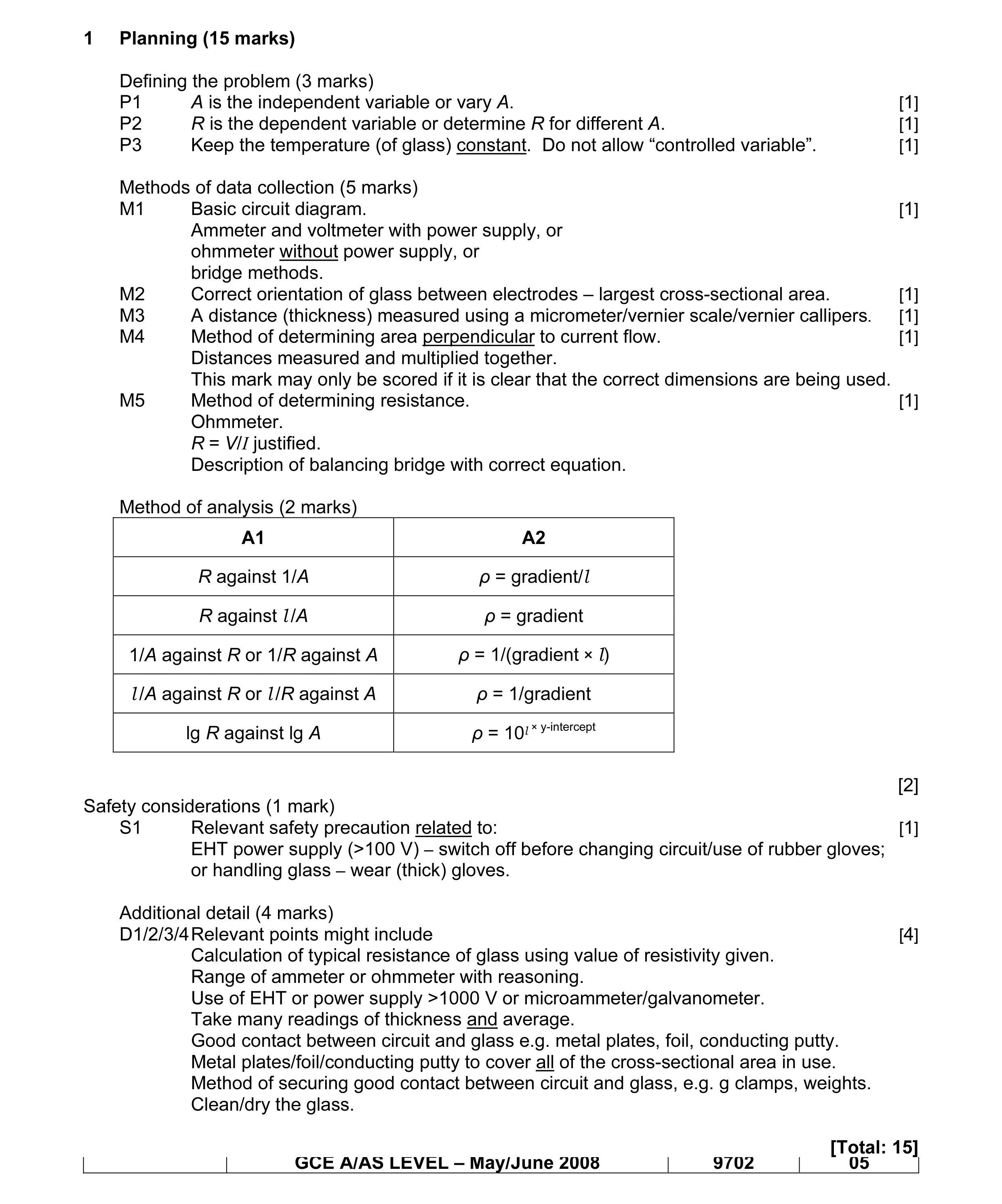 15
15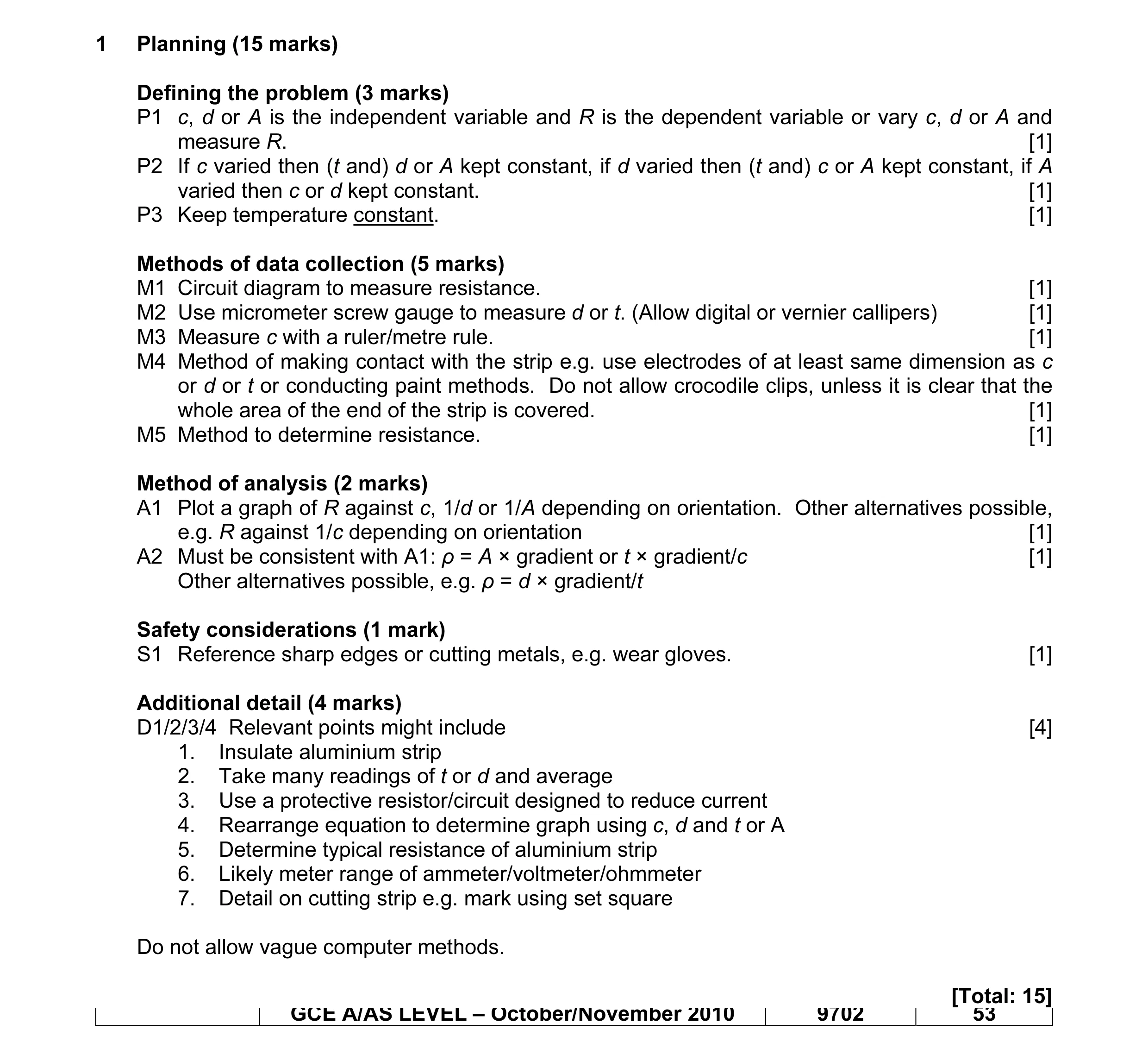 15
15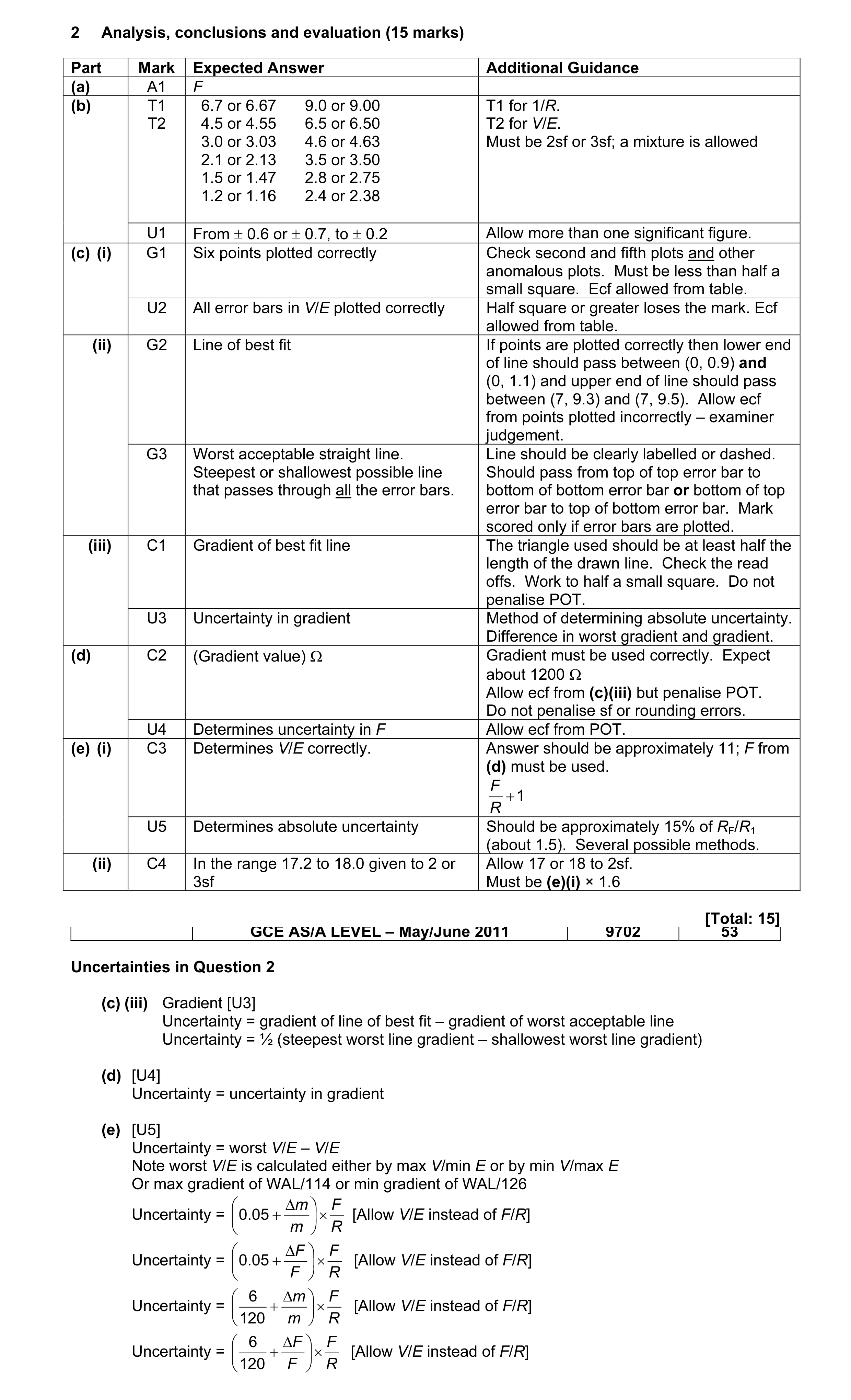 10
10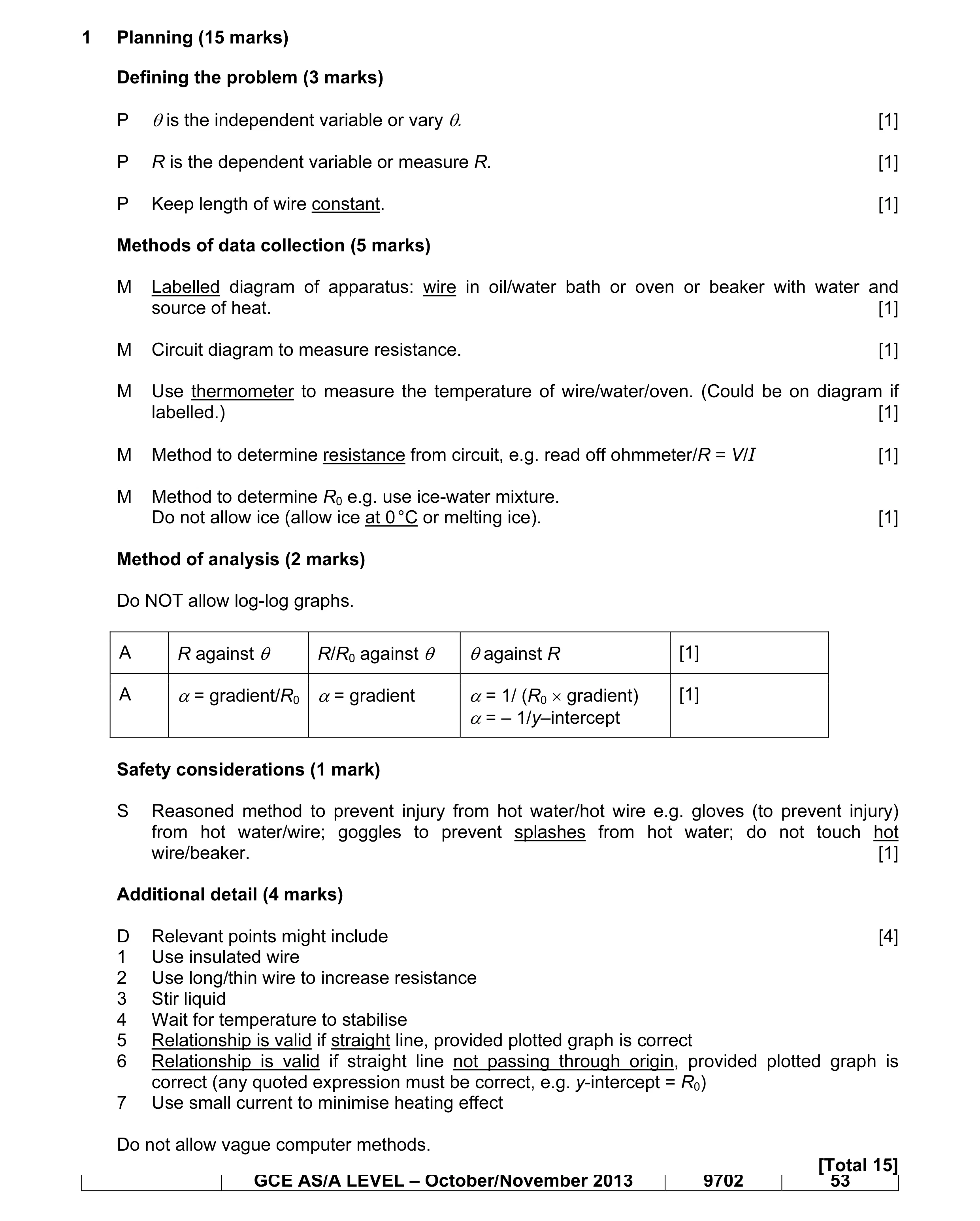 15
15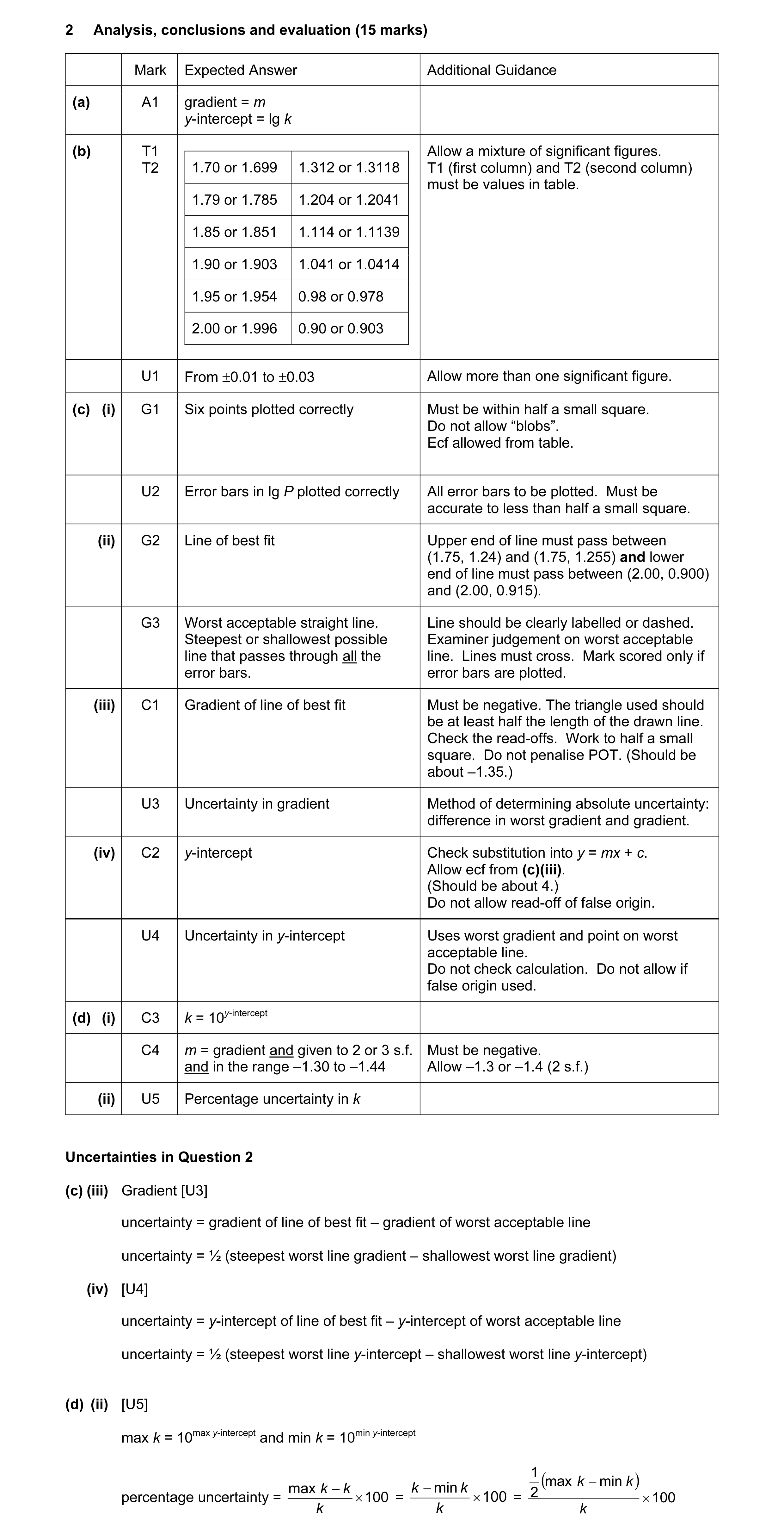 10
10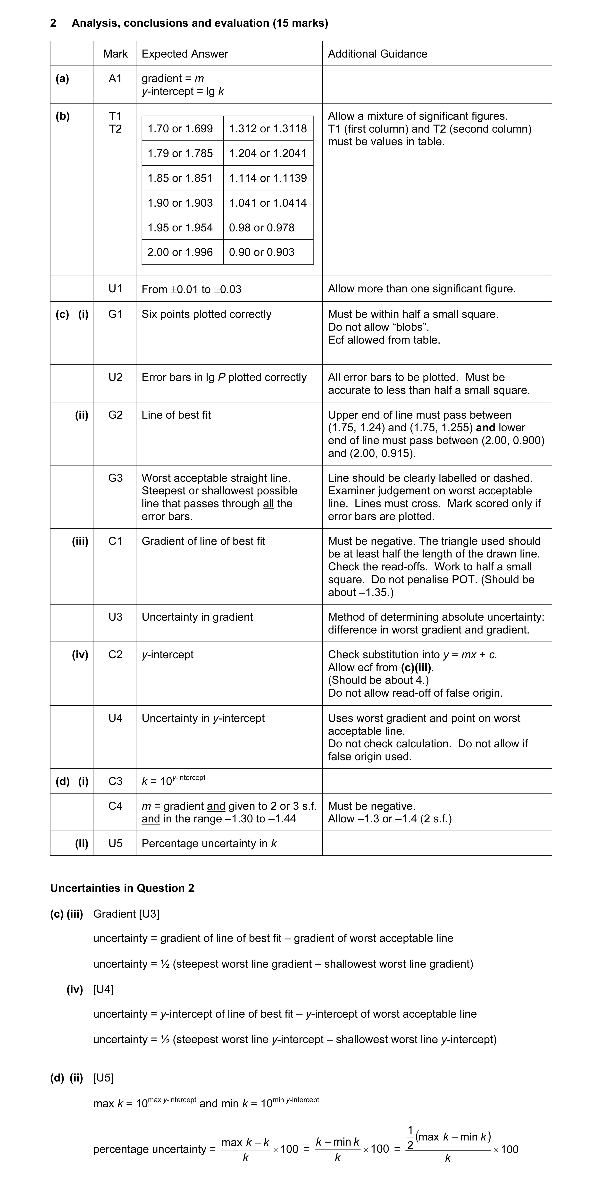 10
10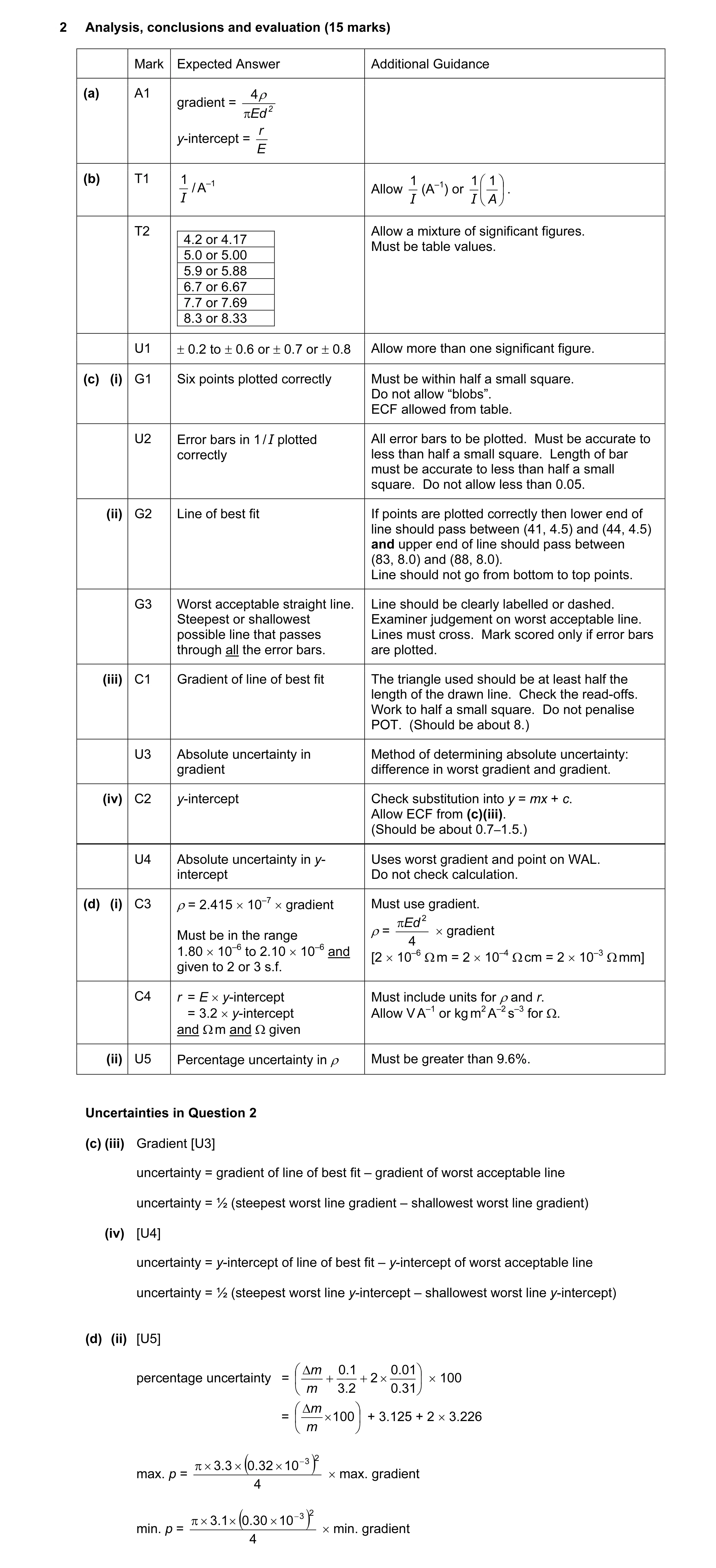 10
10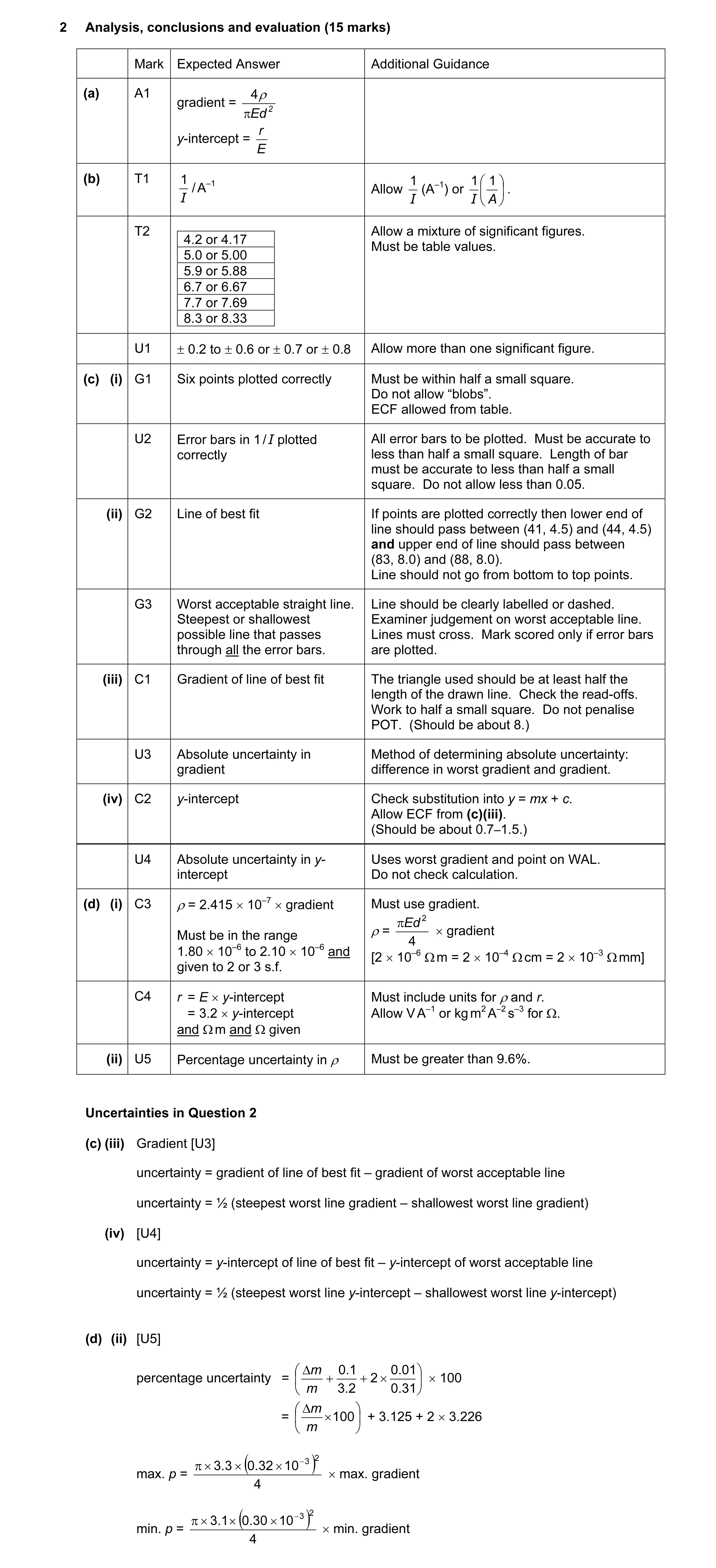 10
10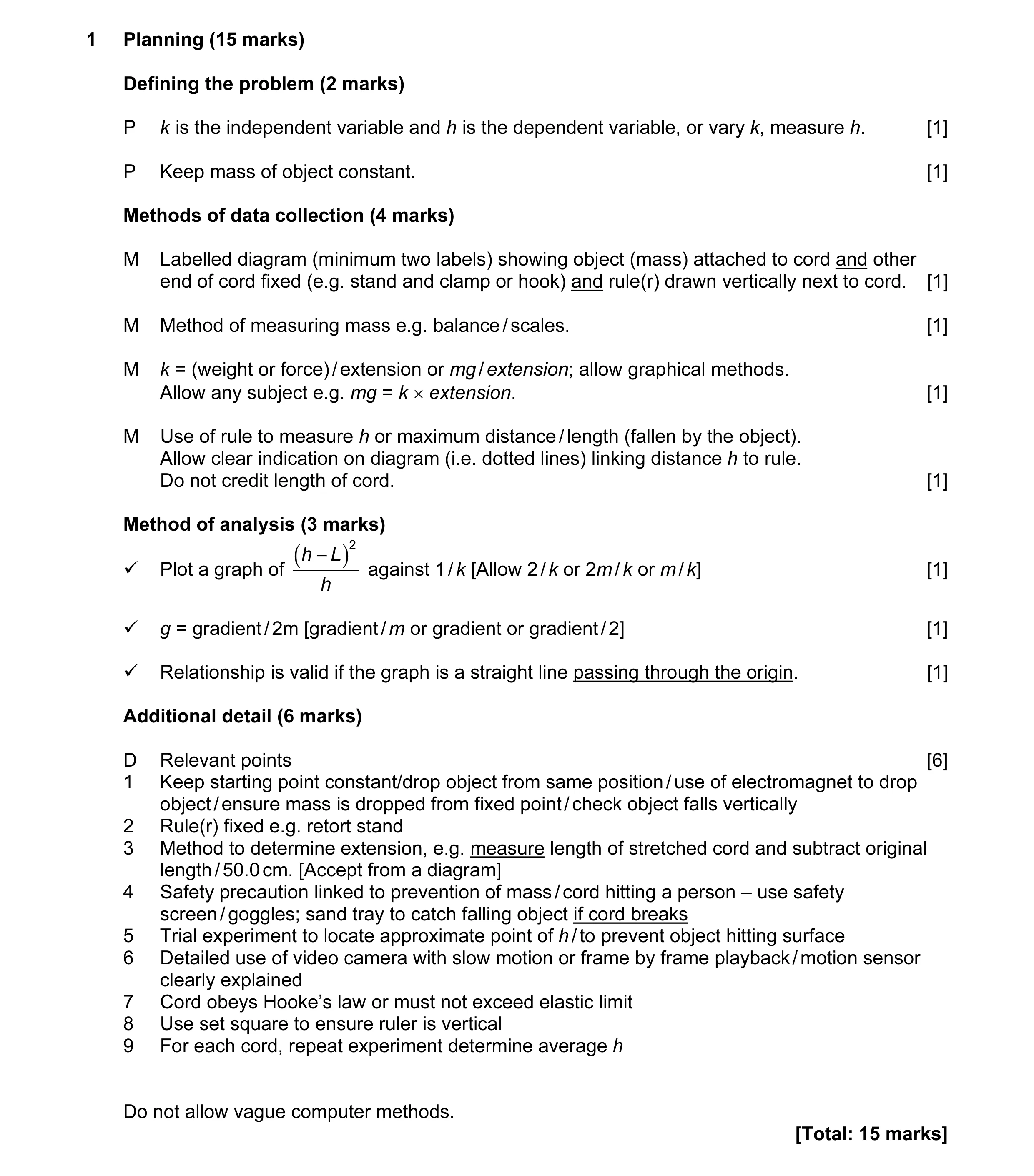 15
15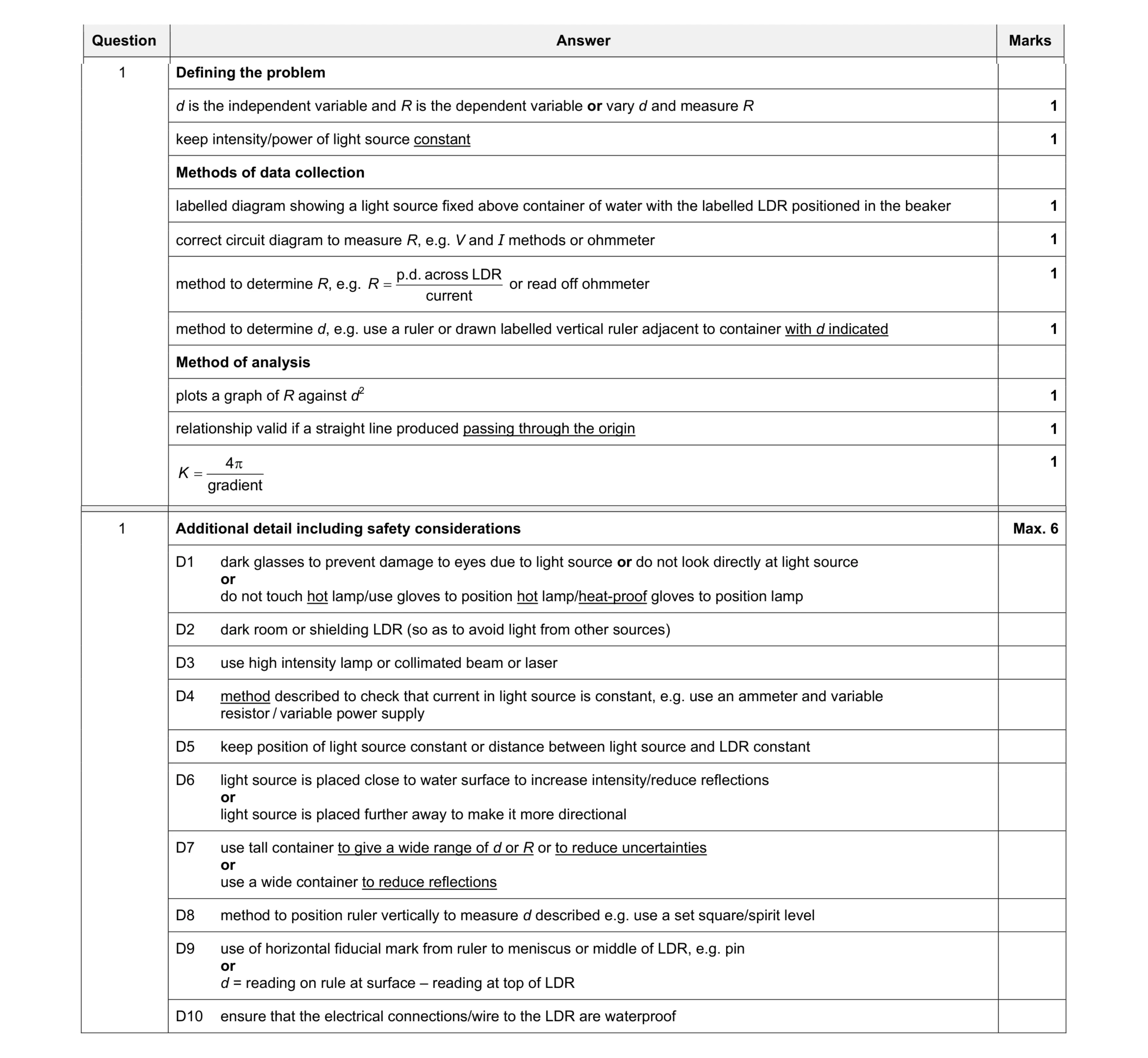 15
15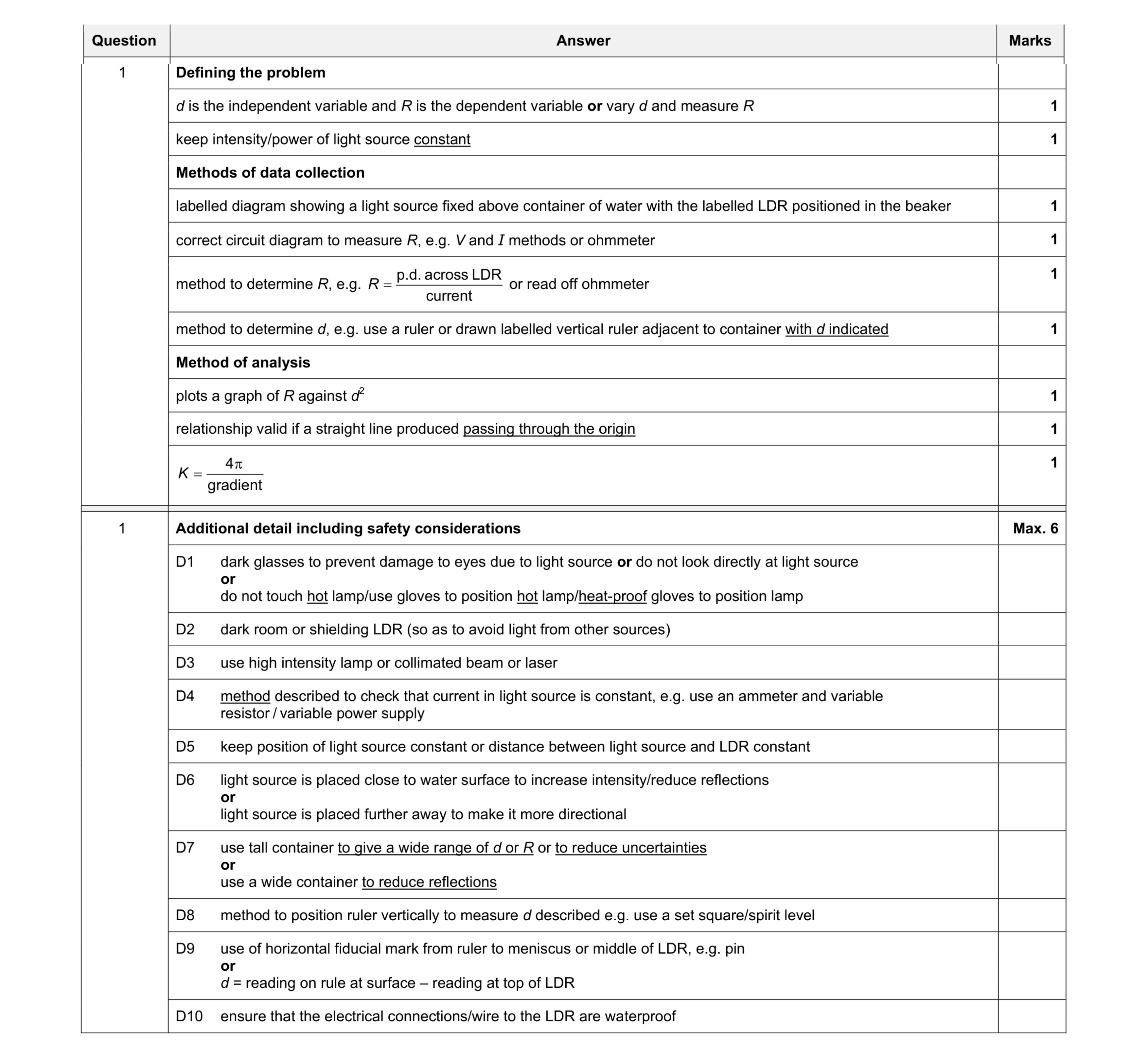 15
15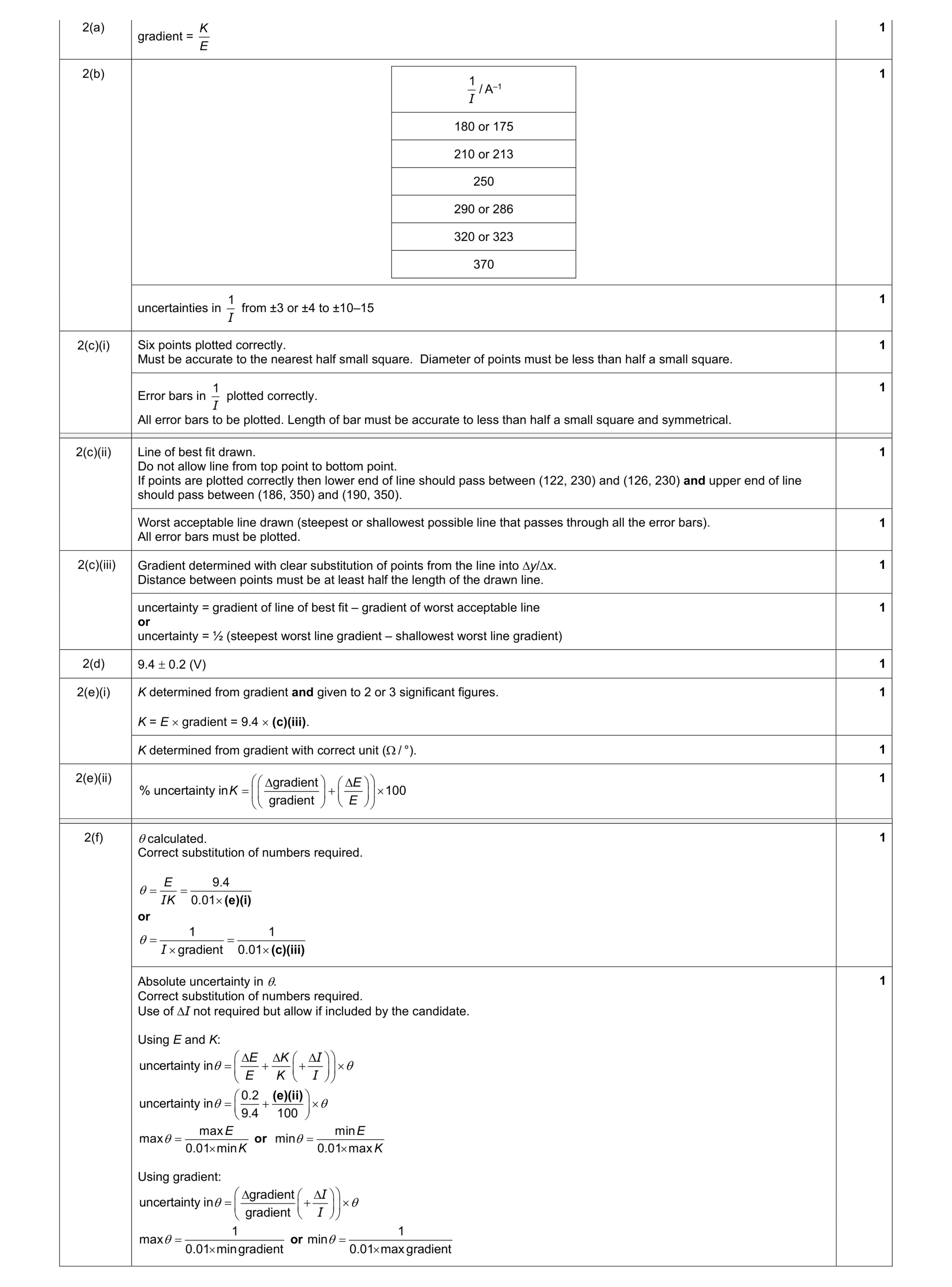 9
9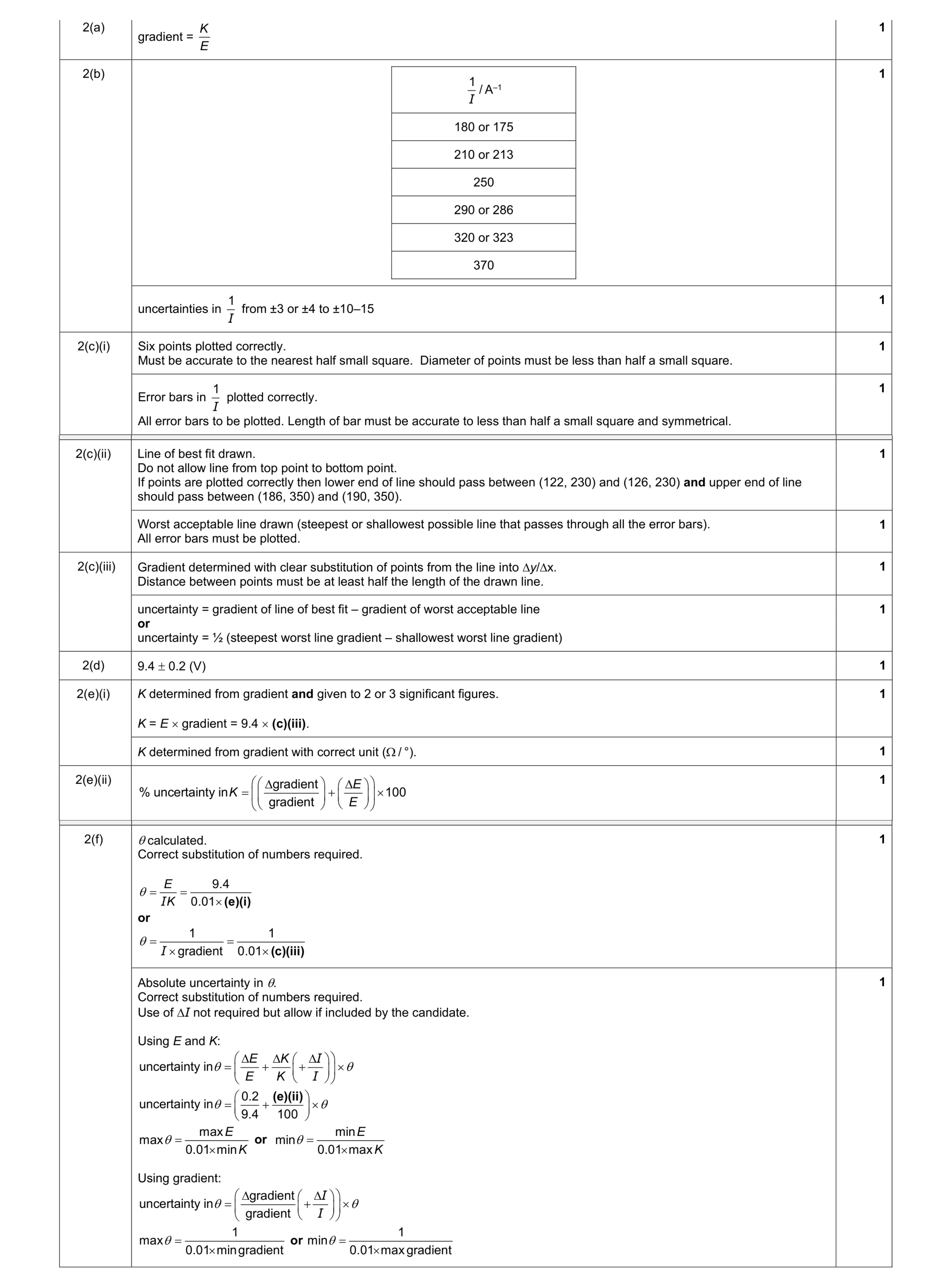 9
9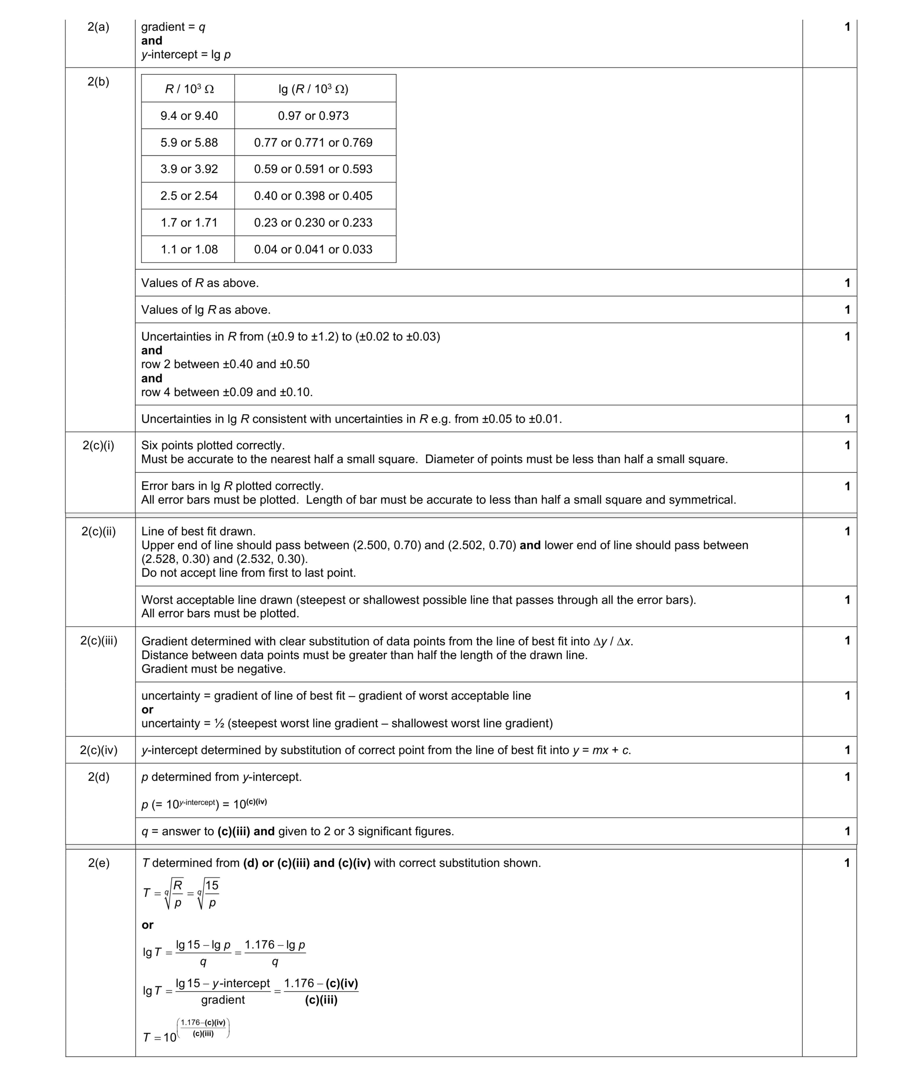 11
11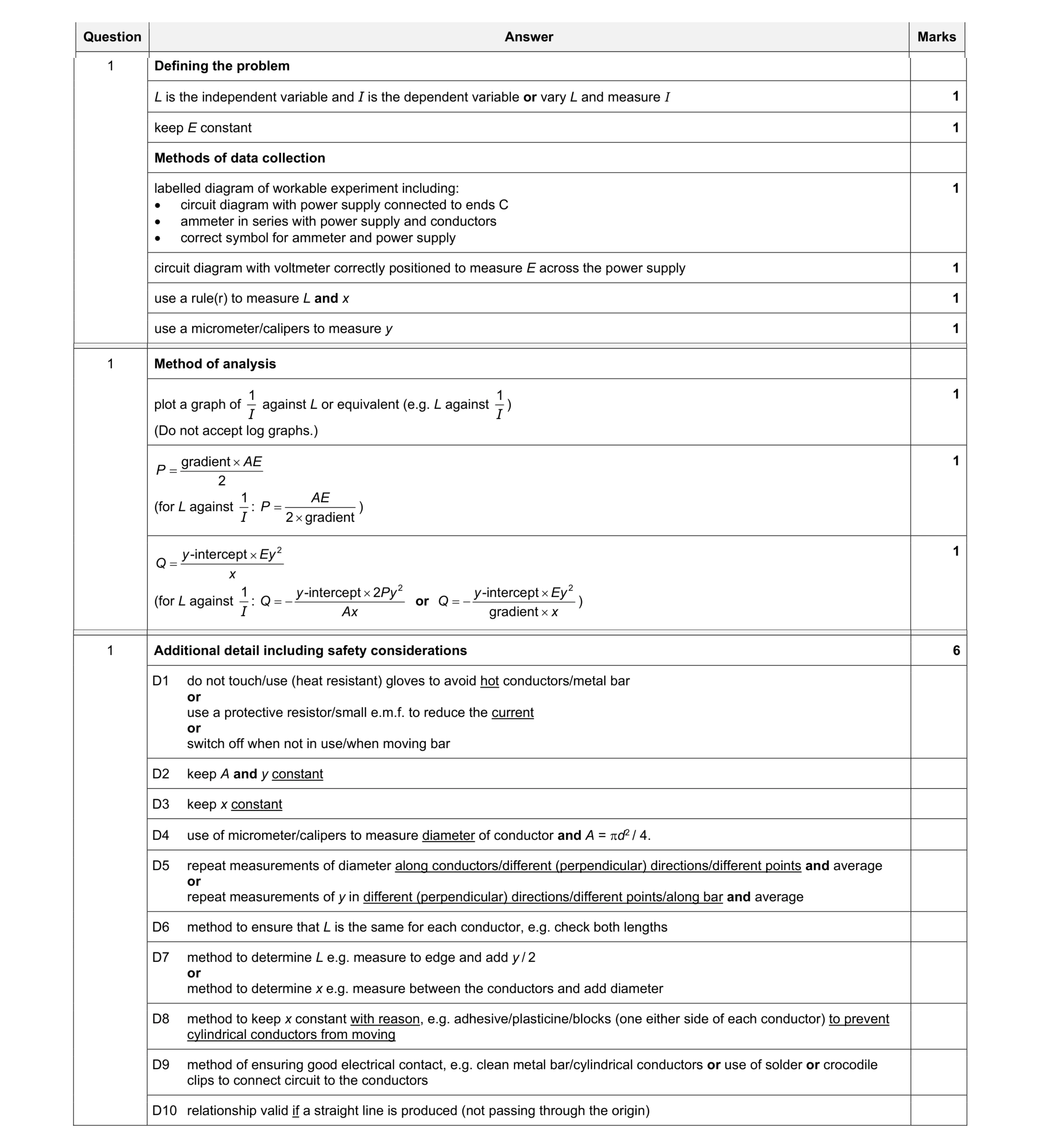 15
15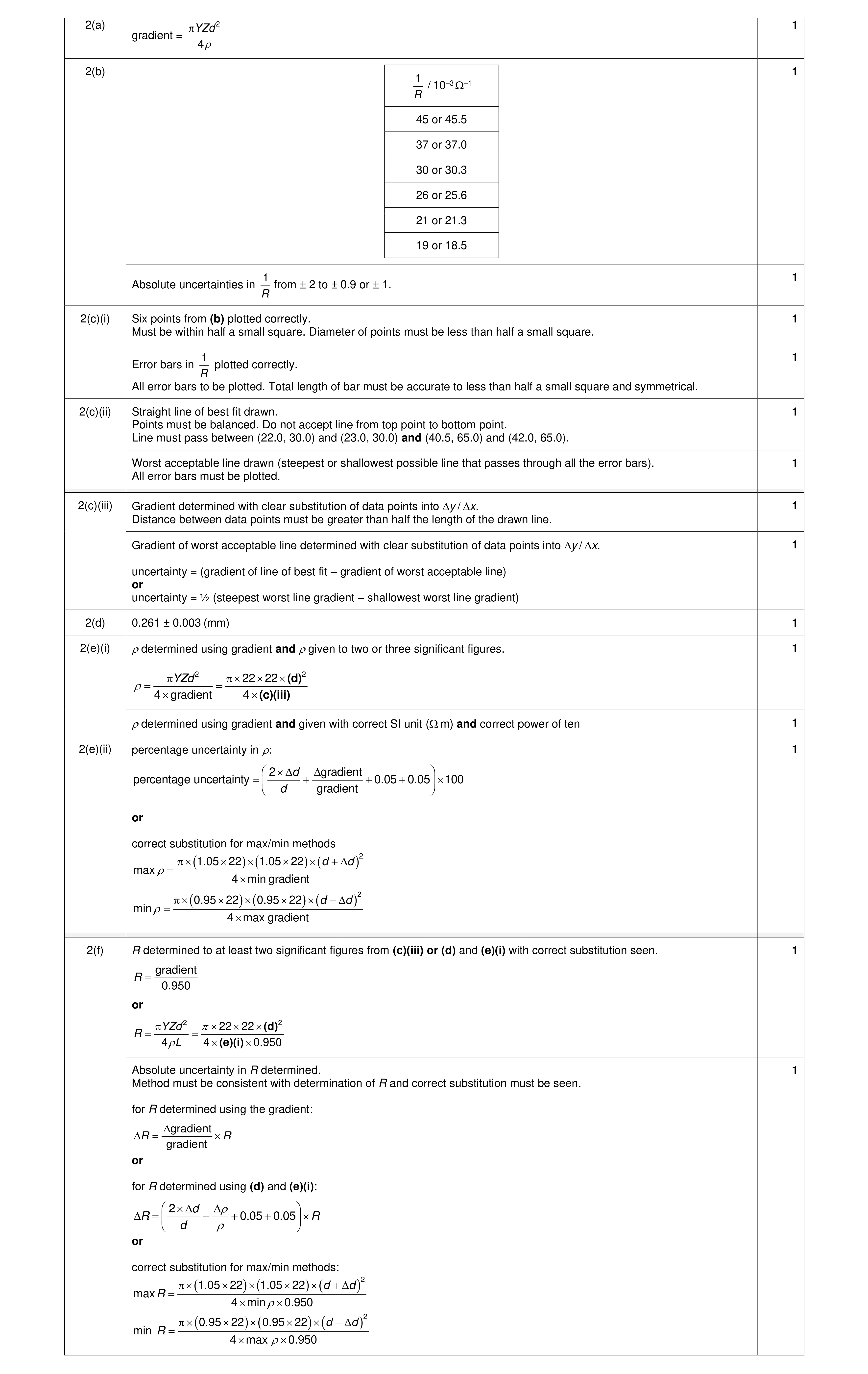 9
9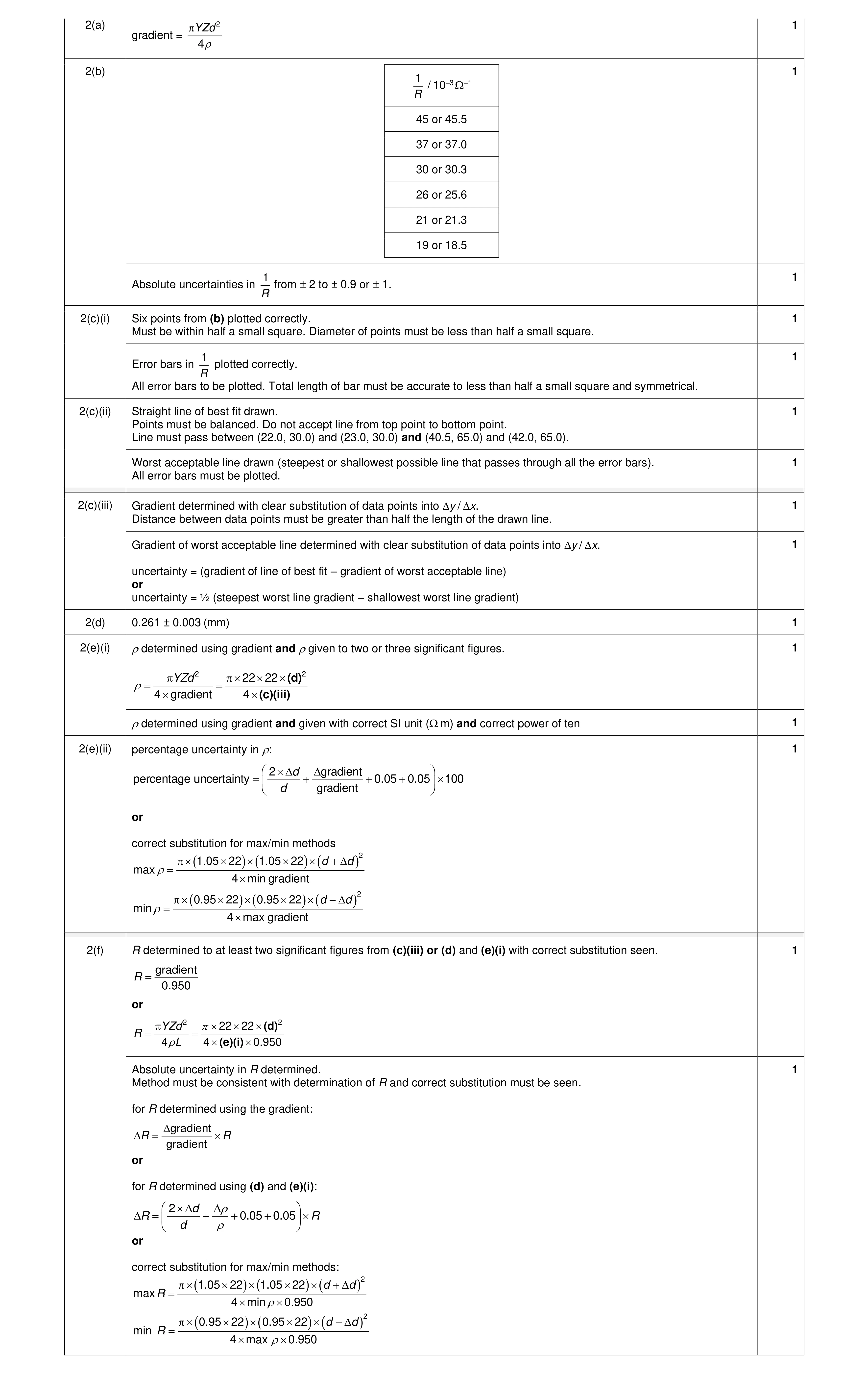 9
9