Cambridge A Level Marine Science 9693 — 2024 May/June Paper 2 · Variant 1
9693/21/M/J/24 · 5 questions · 75 marks · ≈84 min
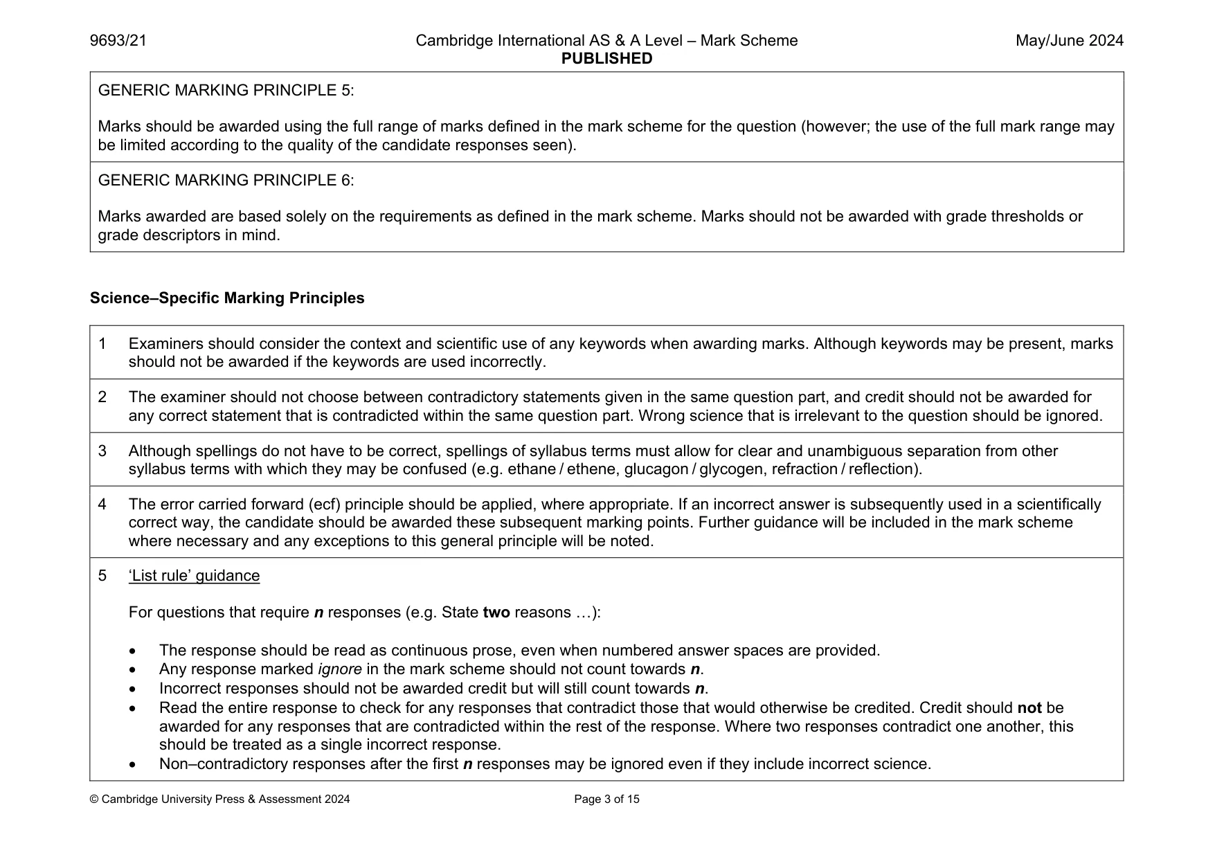
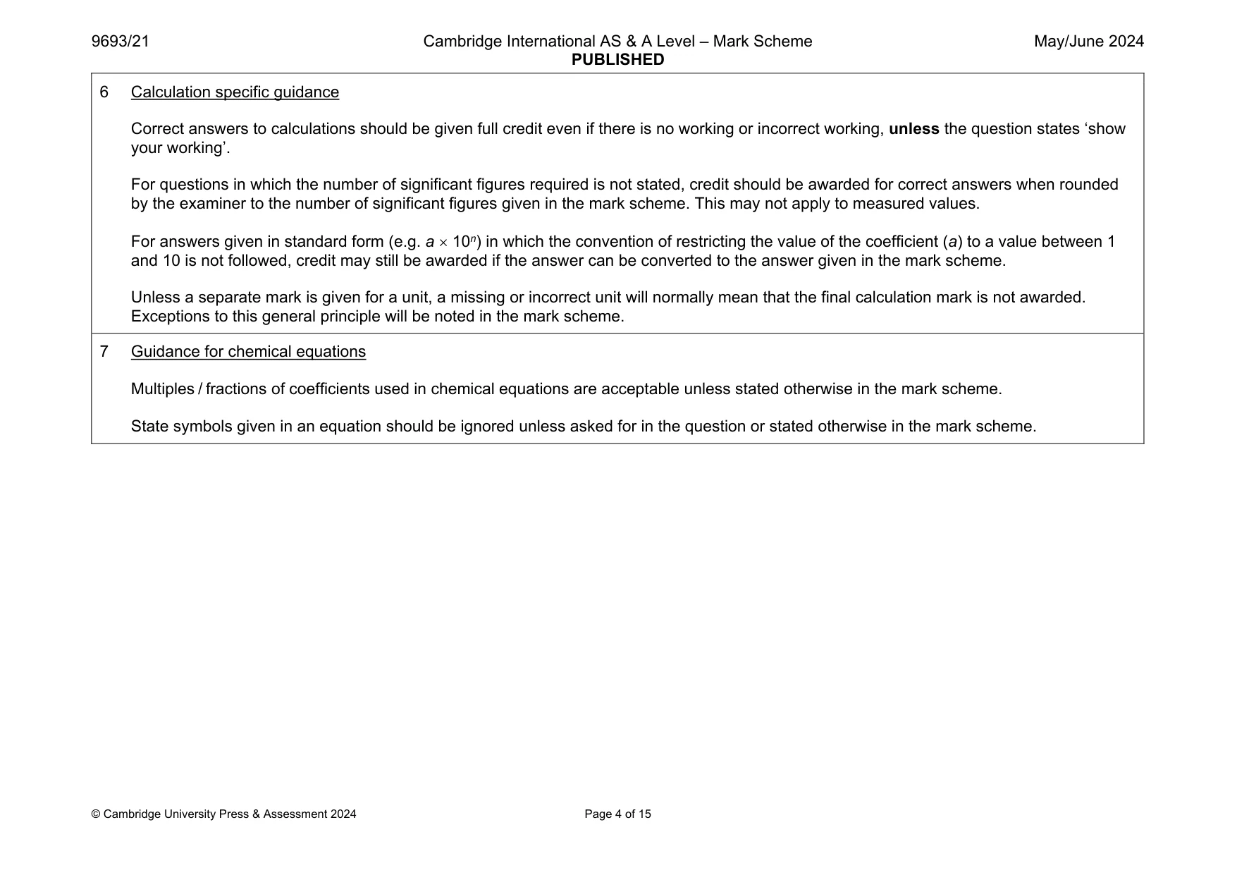
The question paper and its mark scheme, free to read here and free to download. This is Cambridge’s own paper, exactly as it was sat.
Question paper28 pages






Mark scheme15 pages
Answers below. Sit the paper first if you are practising.
Questions as text
Q1 · Zooplankton is composed of a variety of organisms, including copepods
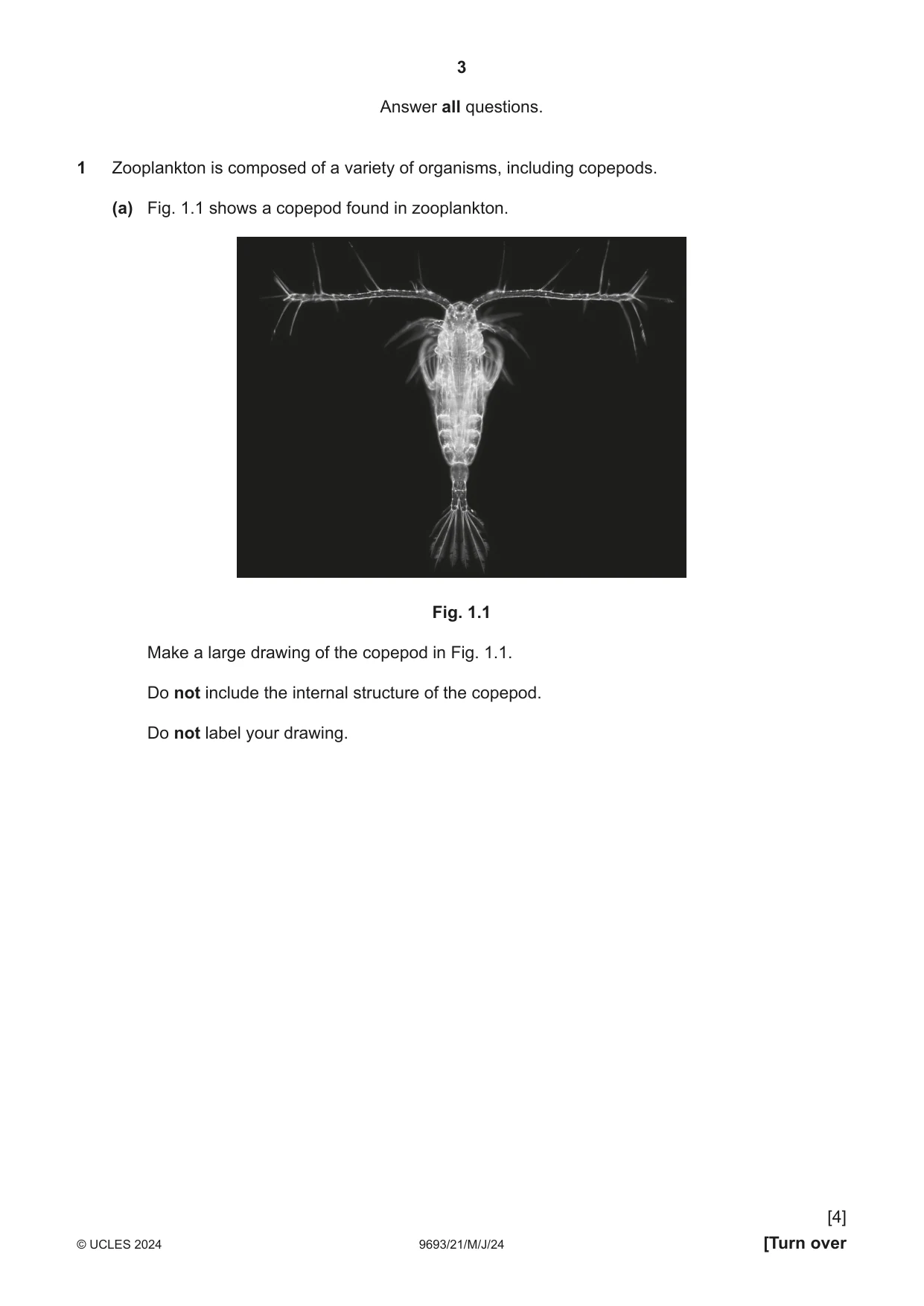
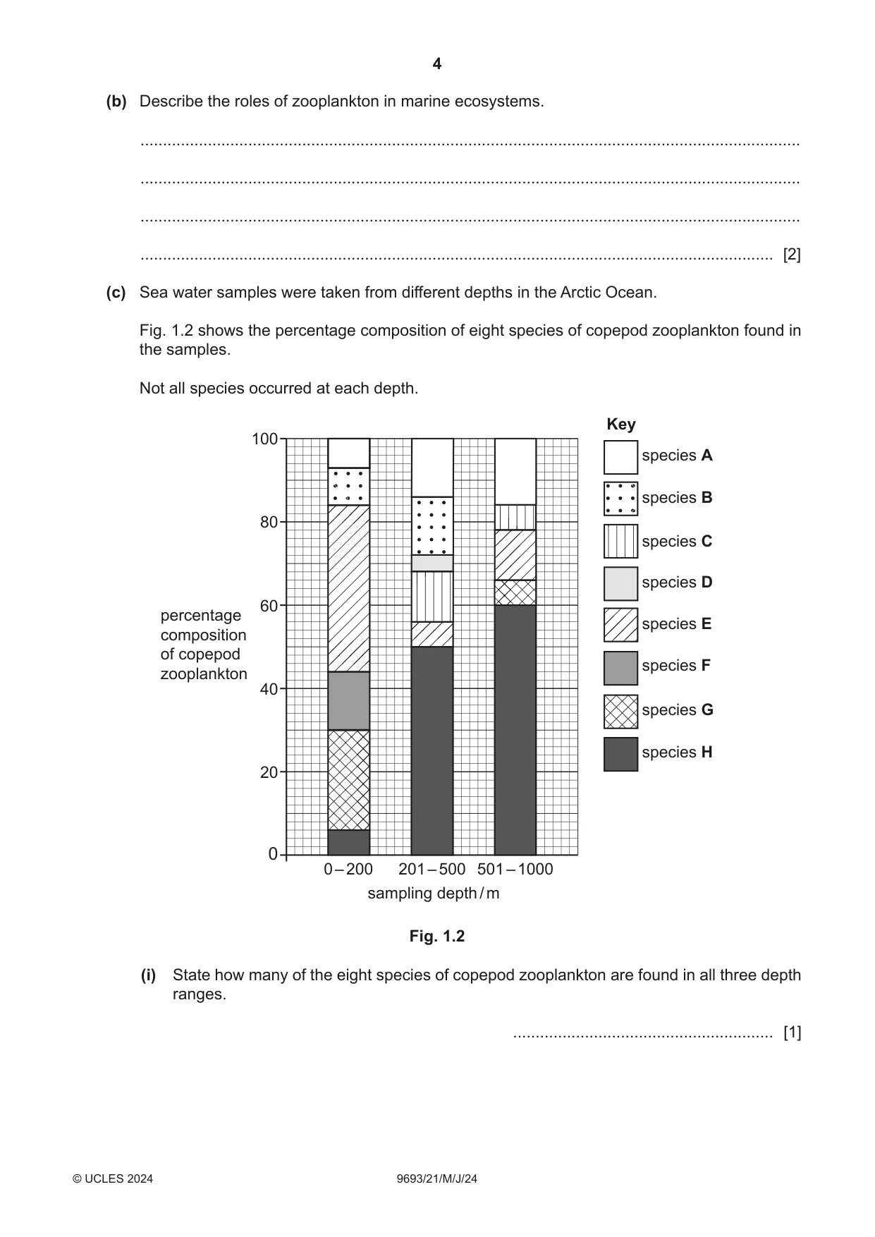
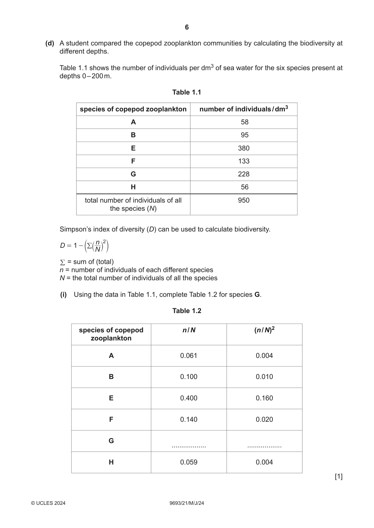
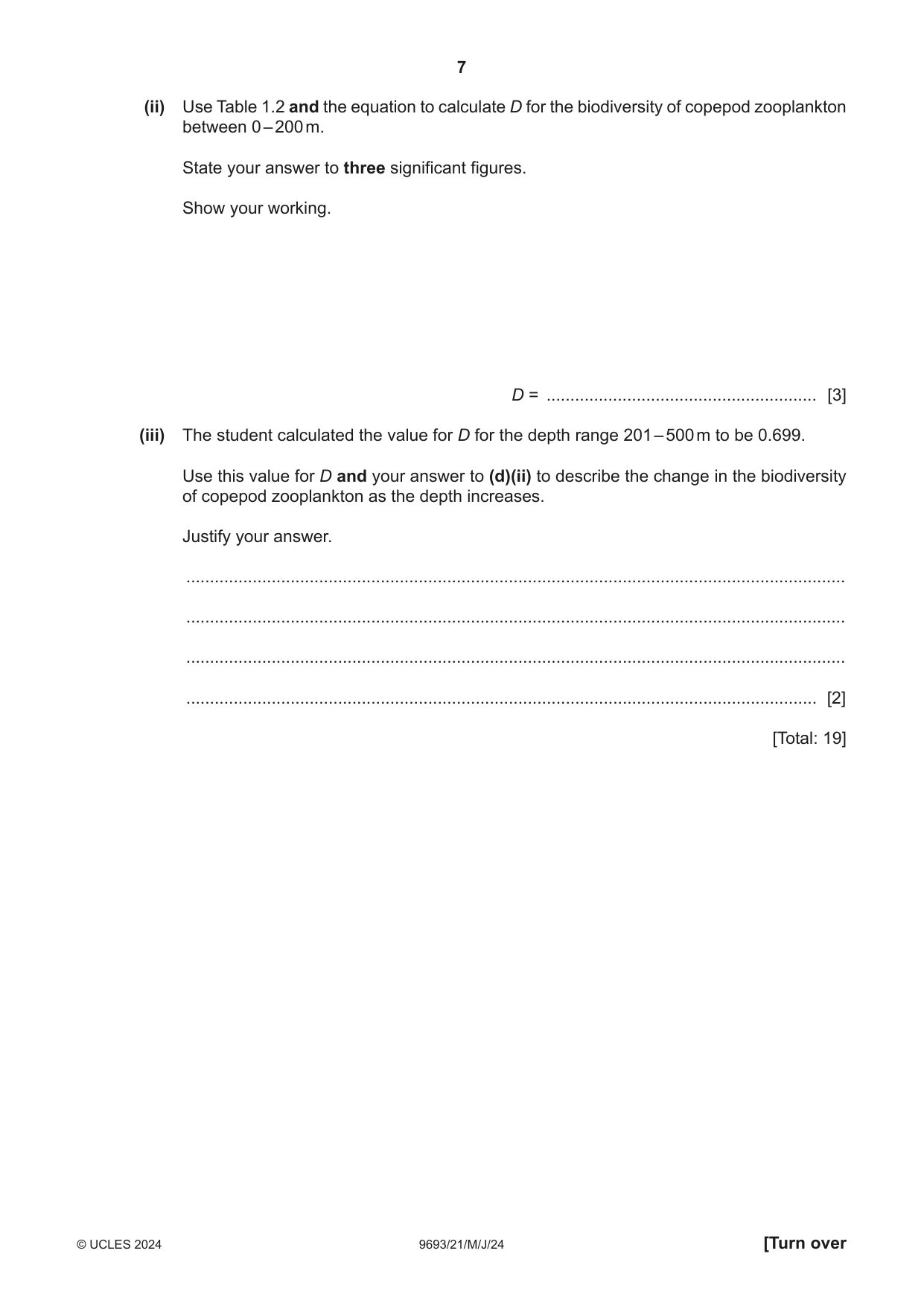
1 Zooplankton is composed of a variety of organisms, including copepods. (a) Fig. 1.1 shows a copepod found in zooplankton. Fig. 1.1 Make a large drawing of the copepod in Fig. 1.1. Do not include the internal structure of the copepod. Do not label your drawing. [4] (b) Describe the roles of zooplankton in marine ecosystems. ................................................................................................................................................... ................................................................................................................................................... ................................................................................................................................................... ............................................................................................................................................. [2] (c) Sea water samples were taken from different depths in the Arctic Ocean. Fig. 1.2 shows the percentage composition of eight species of copepod zooplankton found in the samples. Not all species occurred at each depth. Key 100 species A species B 80 species C species D 60 percentage species E composition of copepod species F zooplankton 40 species G species H 20 0 0 – 200 201 – 500 501 – 1000 sampling depth / m Fig. 1.2 (i) State how many of the eight species of copepod zooplankton are found in all three depth ranges. .......................................................... [1] (ii) Use Fig. 1.2 to compare the changes in percentage composition of species A and species H. ........................................................................................................................................... ........................................................................................................................................... ........................................................................................................................................... ........................................................................................................................................... ........................................................................................................................................... ..................................................................................................................................... [3] (iii) Suggest why the percentage compositions of the copepod zooplankton species change with increasing depth. ........................................................................................................................................... ........................................................................................................................................... ........................................................................................................................................... ........................................................................................................................................... ........................................................................................................................................... ..................................................................................................................................... [3] (d) A student compared the copepod zooplankton communities by calculating the biodiversity at different depths. Table 1.1 shows the number of individuals per dm3 of sea water for the six species present at depths 0 – 200 m. Table 1.1 species of copepod zooplankton number of individuals / dm3 A 58 B 95 E 380 F 133 G 228 H 56 total number of individuals of all 950 the species (N) Simpson’s index of diversity (D) can be used to calculate biodiversity. n 2 D = 1 / N -c ` j m / = sum of (total) n = number of individuals of each different species N = the total number of individuals of all the species (i) Using the data in Table 1.1, complete Table 1.2 for species G. Table 1.2 species of copepod n / N (n / N)2 zooplankton A 0.061 0.004 B 0.100 0.010 E 0.400 0.160 F 0.140 0.020 G .................. .................. H 0.059 0.004 [1] (ii) Use Table 1.2 and the equation to calculate D for the biodiversity of copepod zooplankton between 0 – 200 m. State your answer to three significant figures. Show your working. D = ......................................................... [3] (iii) The student calculated the value for D for the depth range 201 – 500 m to be 0.699. Use this value for D and your answer to (d)(ii) to describe the change in the biodiversity of copepod zooplankton as the depth increases. Justify your answer. ........................................................................................................................................... ........................................................................................................................................... ........................................................................................................................................... ..................................................................................................................................... [2] [Total: 19]
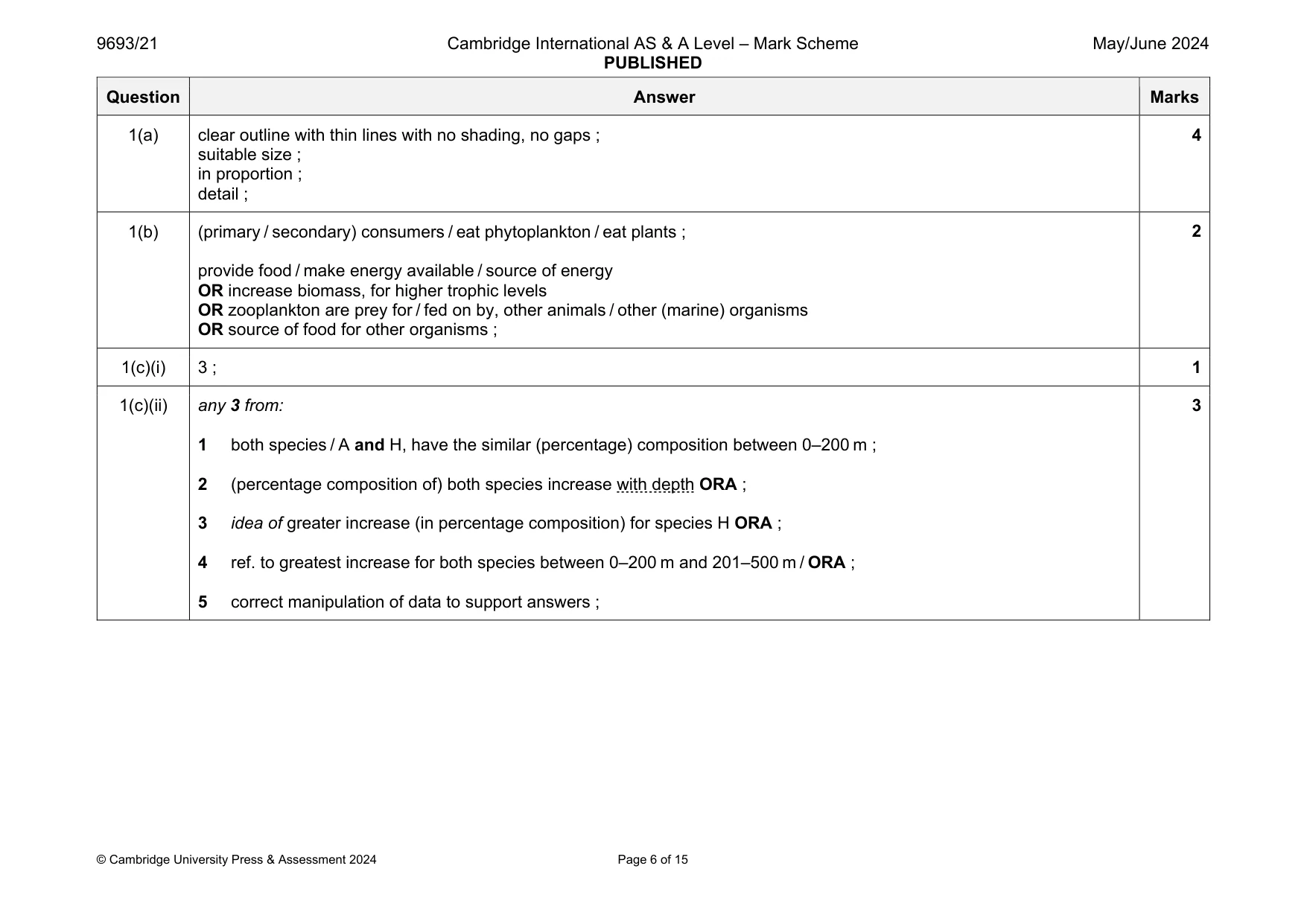
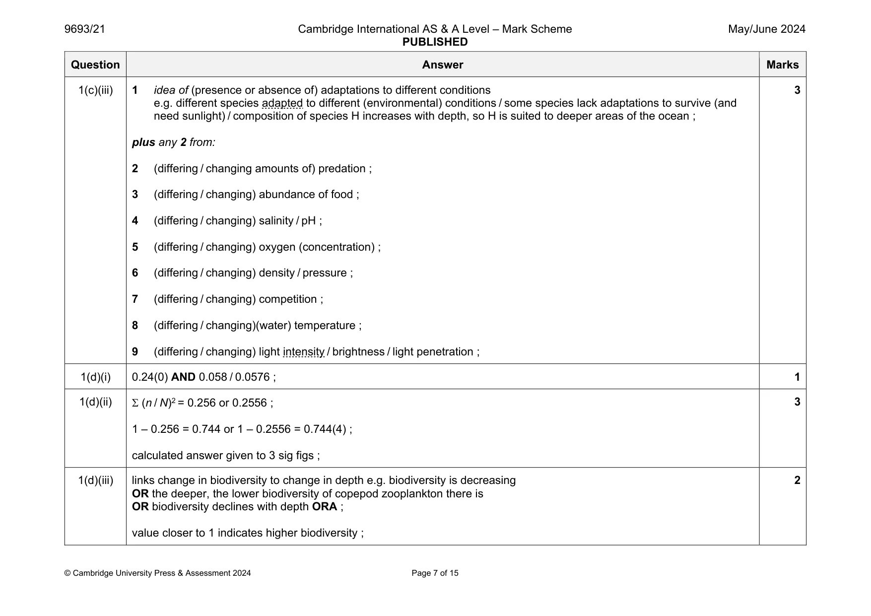
Mark scheme: 1(a) clear outline with thin lines with no shading, no gaps ; suitable size ; in proportion ; detail ; 4 1(b) (primary / secondary) consumers / eat phytoplankton / eat plants ; provide food / make energy available / source of energy OR increase biomass, for higher trophic levels OR zooplankton are prey for / fed on by, other animals / other (marine) organisms OR source of food for other organisms ; 2 1(c)(i) 3 ; 1 1(c)(ii) any 3 from: 1 both species / A and H, have the similar (percentage) composition between 0–200 m ; 2 (percentage composition of) both species increase with depth ORA ; 3 idea of greater increase (in percentage composition) for species H ORA ; 4 ref. to greatest increase for both species between 0–200 m and 201–500 m / ORA ; 5 correct manipulation of data to support answers ; 3 Question Answer Marks 1(c)(iii) 1 idea of (presence or absence of) adaptations to different conditions e.g. different species adapted to different (environmental) conditions / some species lack adaptations to survive (and need sunlight) / composition of species H increases with depth, so H is suited to deeper areas of the ocean ; plus any 2 from: 2 (differing / changing amounts of) predation ; 3 (differing / changing) abundance of food ; 4 (differing / changing) salinity / pH ; 5 (differing / changing) oxygen (concentration) ; 6 (differing / changing) density / pressure ; 7 (differing / changing) competition ; 8 (differing / changing)(water) temperature ; 9 (differing / changing) light intensity / brightness / light penetration ; 3 1(d)(i) 0.24(0) AND 0.058 / 0.0576 ; 1 1(d)(ii) (n / N)2 = 0.256 or 0.2556 ; 1 – 0.256 = 0.744 or 1 – 0.2556 = 0.744(4) ; calculated answer given to 3 sig figs ; 3 1(d)(iii) links change in biodiversity to change in depth e.g. biodiversity is decreasing OR the deeper, the lower biodiversity of copepod zooplankton there is OR biodiversity declines with depth ORA ; value closer to 1 indicates higher biodiversity ; 2
Q2 · A student investigated photosynthesis in three species of macroalga, P, Q and R
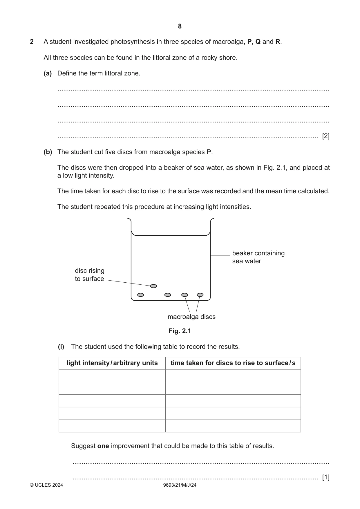
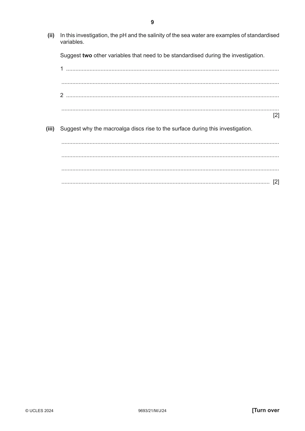
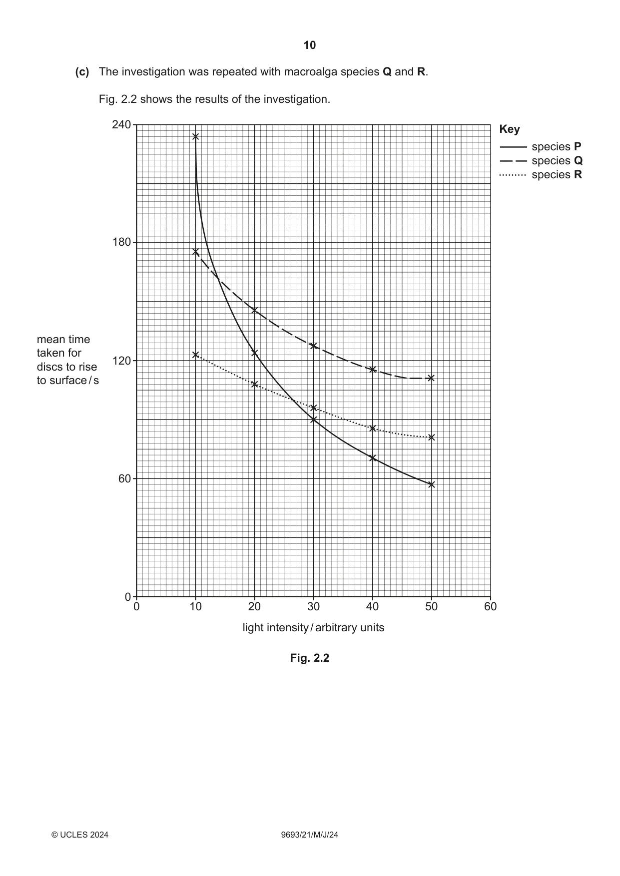
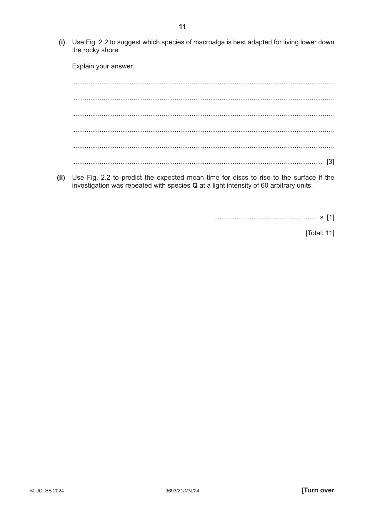
2 A student investigated photosynthesis in three species of macroalga, P, Q and R. All three species can be found in the littoral zone of a rocky shore. (a) Define the term littoral zone. ................................................................................................................................................... ................................................................................................................................................... ................................................................................................................................................... ............................................................................................................................................. [2] (b) The student cut five discs from macroalga species P. The discs were then dropped into a beaker of sea water, as shown in Fig. 2.1, and placed at a low light intensity. The time taken for each disc to rise to the surface was recorded and the mean time calculated. The student repeated this procedure at increasing light intensities. beaker containing sea water disc rising to surface macroalga discs Fig. 2.1 (i) The student used the following table to record the results. light intensity / arbitrary units time taken for discs to rise to surface / s Suggest one improvement that could be made to this table of results. ........................................................................................................................................... ..................................................................................................................................... [1] (ii) In this investigation, the pH and the salinity of the sea water are examples of standardised variables. Suggest two other variables that need to be standardised during the investigation. 1 ........................................................................................................................................ ........................................................................................................................................... 2 ........................................................................................................................................ ........................................................................................................................................... [2] (iii) Suggest why the macroalga discs rise to the surface during this investigation. ........................................................................................................................................... ........................................................................................................................................... ........................................................................................................................................... ..................................................................................................................................... [2] (c) The investigation was repeated with macroalga species Q and R. Fig. 2.2 shows the results of the investigation. 240 Key species P species Q species R 180 mean time taken for 120discs to rise to surface / s 60 0 0 10 20 30 40 50 60 light intensity / arbitrary units Fig. 2.2 (i) Use Fig. 2.2 to suggest which species of macroalga is best adapted for living lower down the rocky shore. Explain your answer. ........................................................................................................................................... ........................................................................................................................................... ........................................................................................................................................... ........................................................................................................................................... ........................................................................................................................................... ..................................................................................................................................... [3] (ii) Use Fig. 2.2 to predict the expected mean time for discs to rise to the surface if the investigation was repeated with species Q at a light intensity of 60 arbitrary units. ........................................................ s [1] [Total: 11]
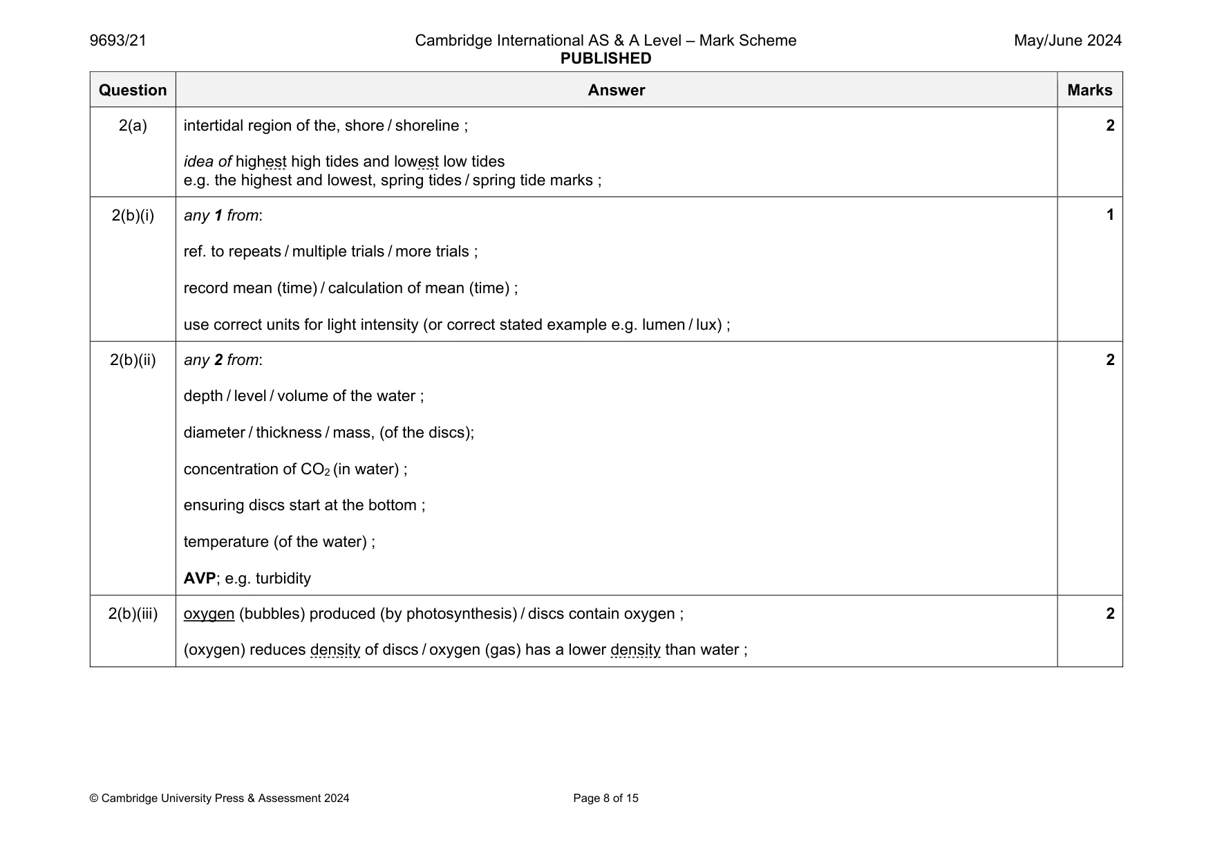
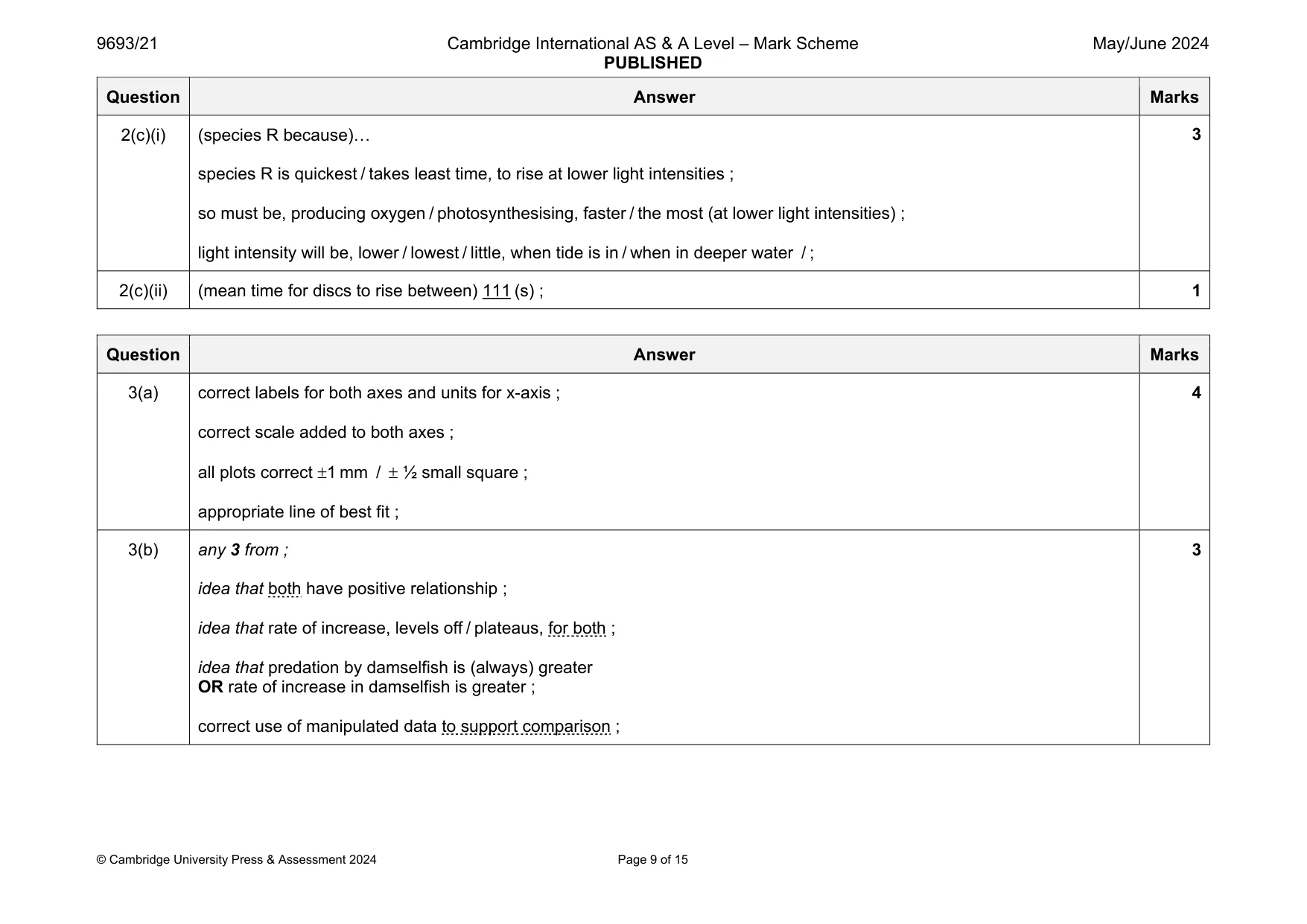
Mark scheme: 2(a) intertidal region of the, shore / shoreline ; idea of highest high tides and lowest low tides e.g. the highest and lowest, spring tides / spring tide marks ; 2 2(b)(i) any 1 from: ref. to repeats / multiple trials / more trials ; record mean (time) / calculation of mean (time) ; use correct units for light intensity (or correct stated example e.g. lumen / lux) ; 1 2(b)(ii) any 2 from: depth / level / volume of the water ; diameter / thickness / mass, (of the discs); concentration of CO2 (in water) ; ensuring discs start at the bottom ; temperature (of the water) ; AVP; e.g. turbidity 2 2(b)(iii) oxygen (bubbles) produced (by photosynthesis) / discs contain oxygen ; (oxygen) reduces density of discs / oxygen (gas) has a lower density than water ; 2 Question Answer Marks 2(c)(i) (species R because)… species R is quickest / takes least time, to rise at lower light intensities ; so must be, producing oxygen / photosynthesising, faster / the most (at lower light intensities) ; light intensity will be, lower / lowest / little, when tide is in / when in deeper water / ; 3 2(c)(ii) (mean time for discs to rise between) 111 (s) ; 1
Q3 · Damselfish and wrasse are two types of small predatory fish found on tropical coral…
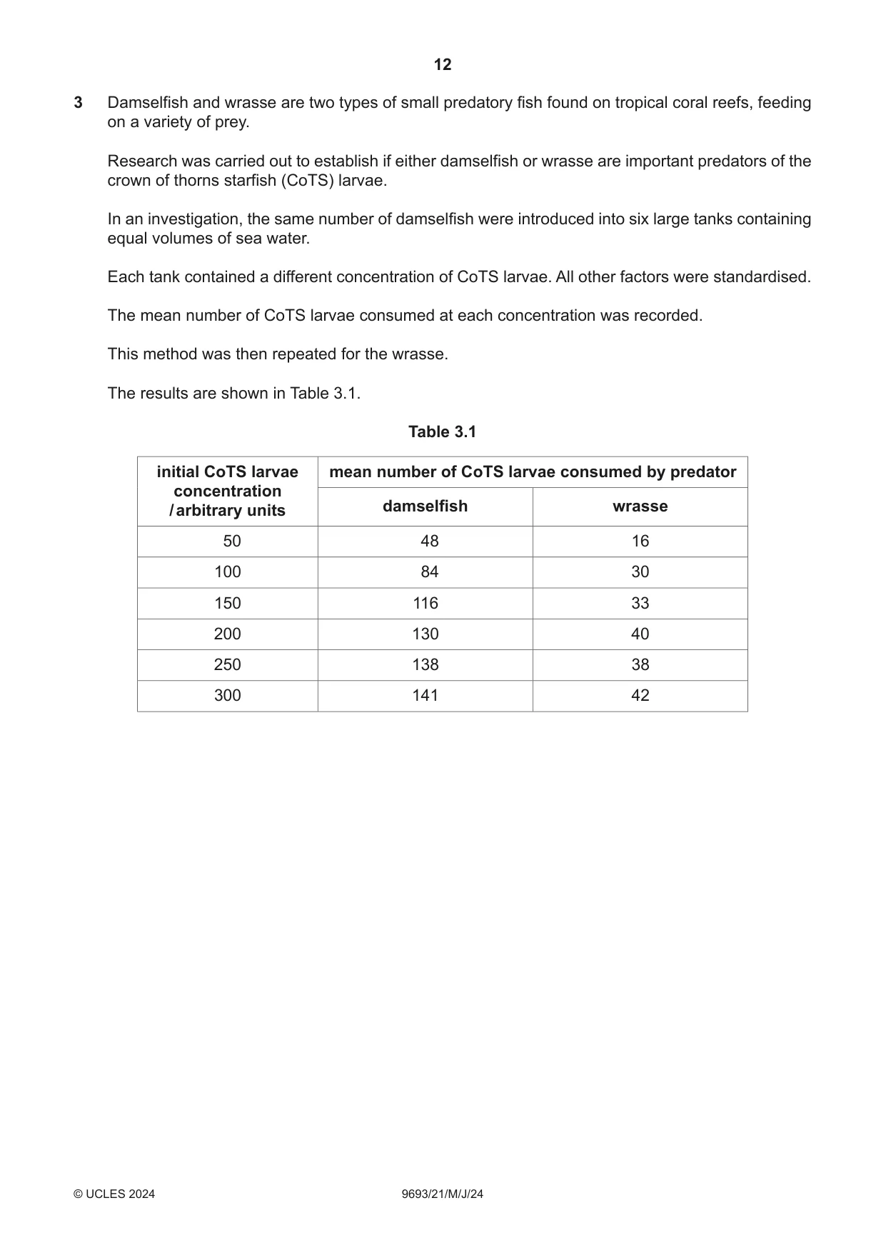
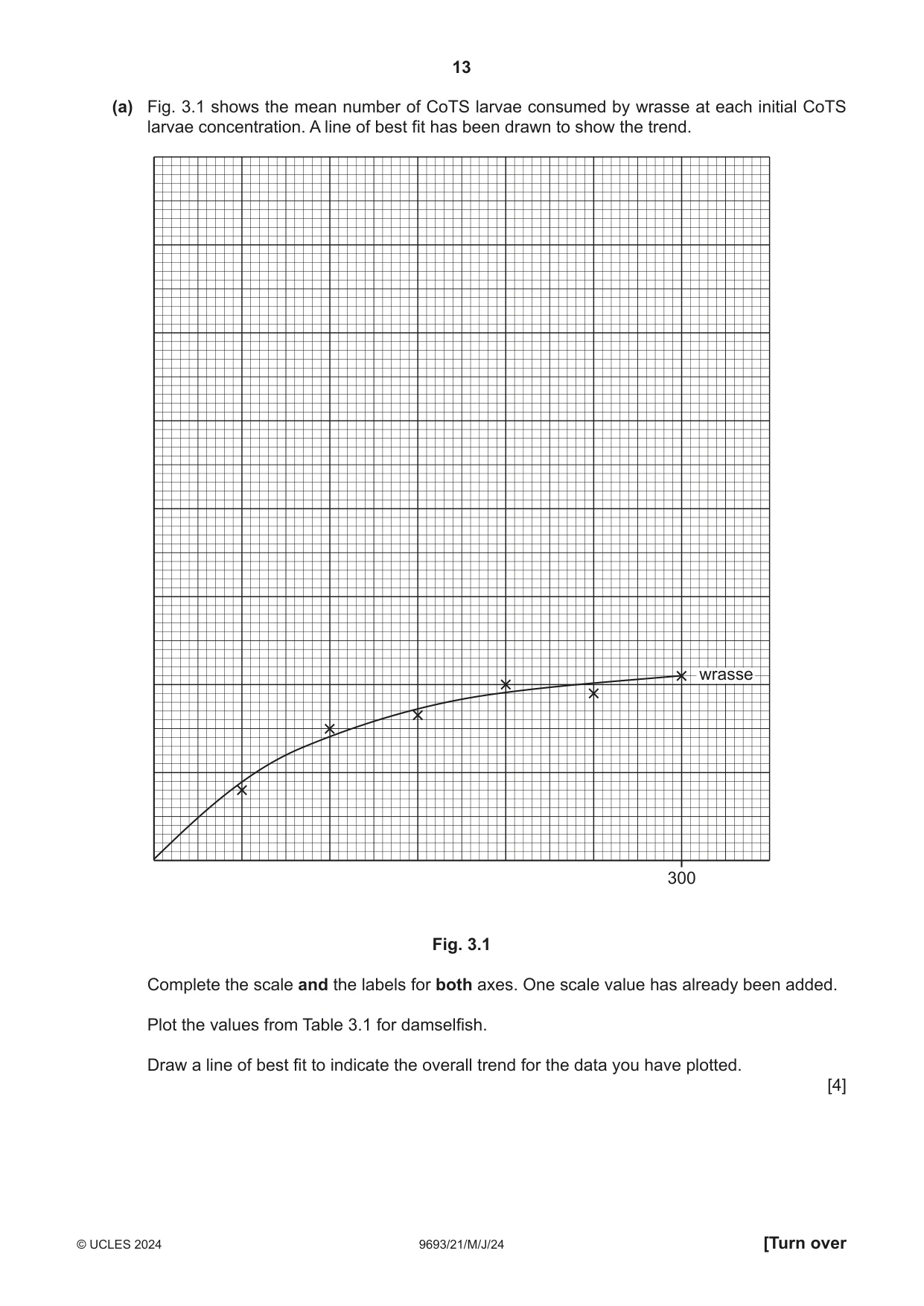
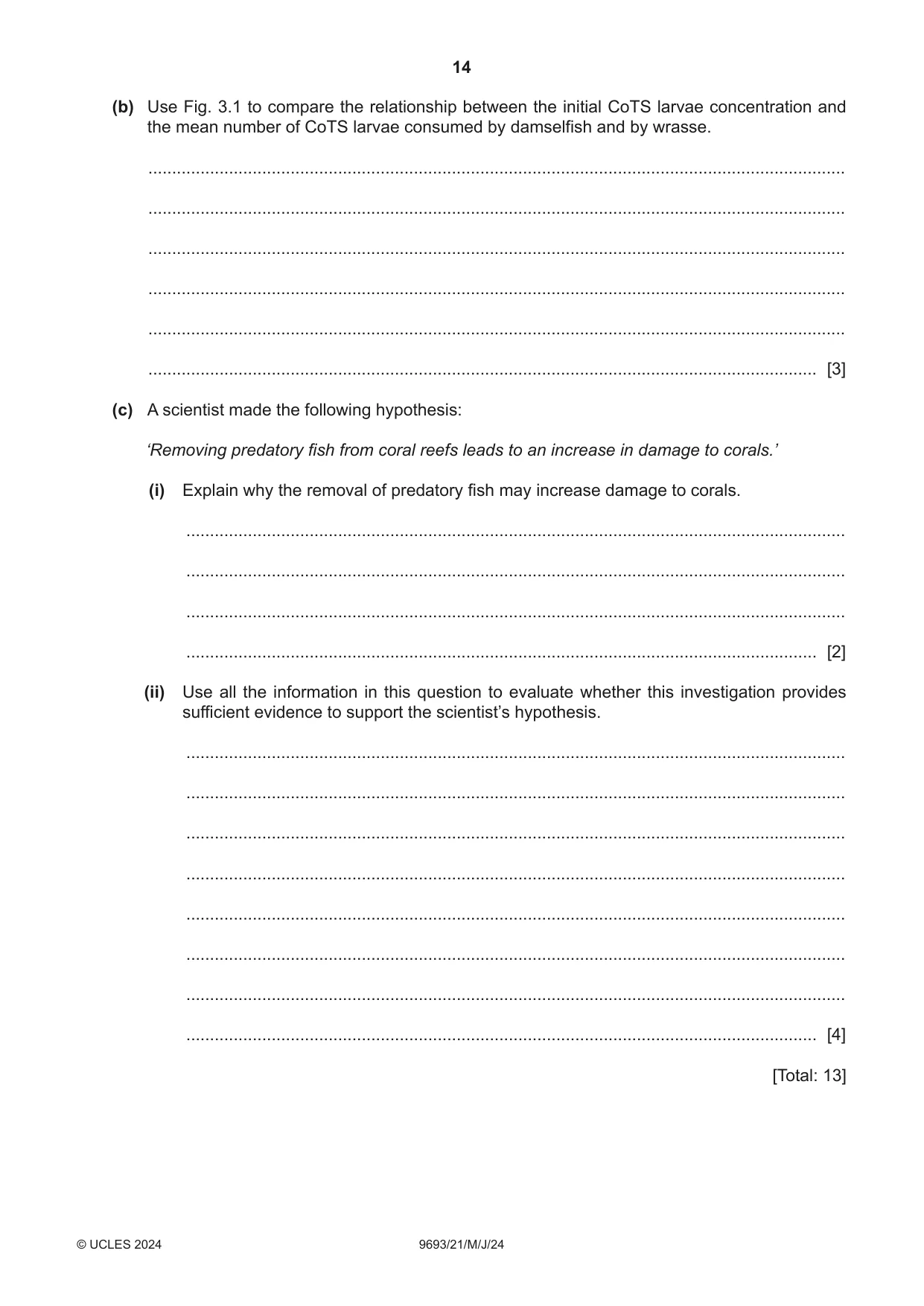
3 Damselfish and wrasse are two types of small predatory fish found on tropical coral reefs, feeding on a variety of prey. Research was carried out to establish if either damselfish or wrasse are important predators of the crown of thorns starfish (CoTS) larvae. In an investigation, the same number of damselfish were introduced into six large tanks containing equal volumes of sea water. Each tank contained a different concentration of CoTS larvae. All other factors were standardised. The mean number of CoTS larvae consumed at each concentration was recorded. This method was then repeated for the wrasse. The results are shown in Table 3.1. Table 3.1 initial CoTS larvae mean number of CoTS larvae consumed by predator concentration / arbitrary units damselfish wrasse 50 48 16 100 84 30 150 116 33 200 130 40 250 138 38 300 141 42 (a) Fig. 3.1 shows the mean number of CoTS larvae consumed by wrasse at each initial CoTS larvae concentration. A line of best fit has been drawn to show the trend. wrasse 300 Fig. 3.1 Complete the scale and the labels for both axes. One scale value has already been added. Plot the values from Table 3.1 for damselfish. Draw a line of best fit to indicate the overall trend for the data you have plotted. [4] (b) Use Fig. 3.1 to compare the relationship between the initial CoTS larvae concentration and the mean number of CoTS larvae consumed by damselfish and by wrasse. ................................................................................................................................................... ................................................................................................................................................... ................................................................................................................................................... ................................................................................................................................................... ................................................................................................................................................... ............................................................................................................................................. [3] (c) A scientist made the following hypothesis: ‘Removing predatory fish from coral reefs leads to an increase in damage to corals.’ (i) Explain why the removal of predatory fish may increase damage to corals. ........................................................................................................................................... ........................................................................................................................................... ........................................................................................................................................... ..................................................................................................................................... [2] (ii) Use all the information in this question to evaluate whether this investigation provides sufficient evidence to support the scientist’s hypothesis. ........................................................................................................................................... ........................................................................................................................................... ........................................................................................................................................... ........................................................................................................................................... ........................................................................................................................................... ........................................................................................................................................... ........................................................................................................................................... ..................................................................................................................................... [4] [Total: 13]
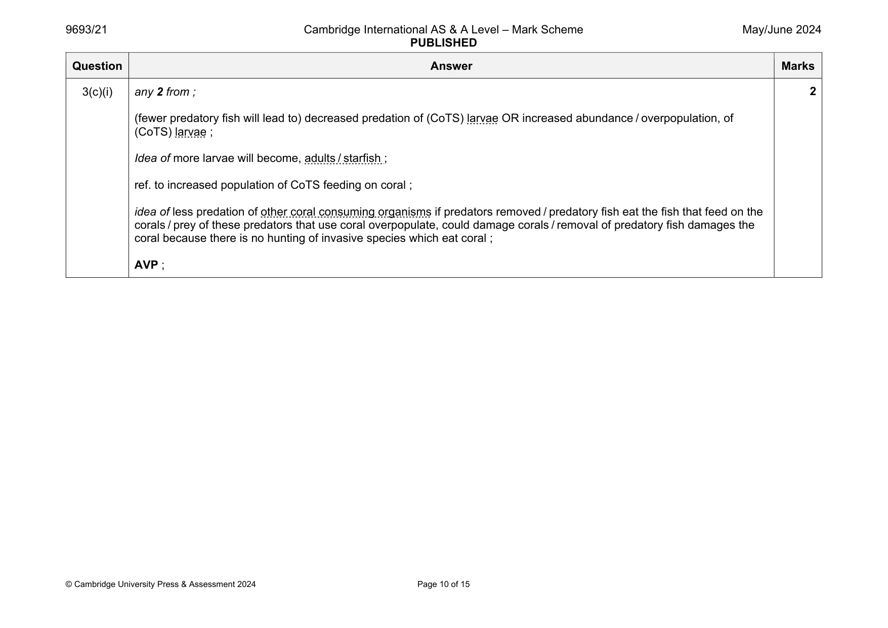
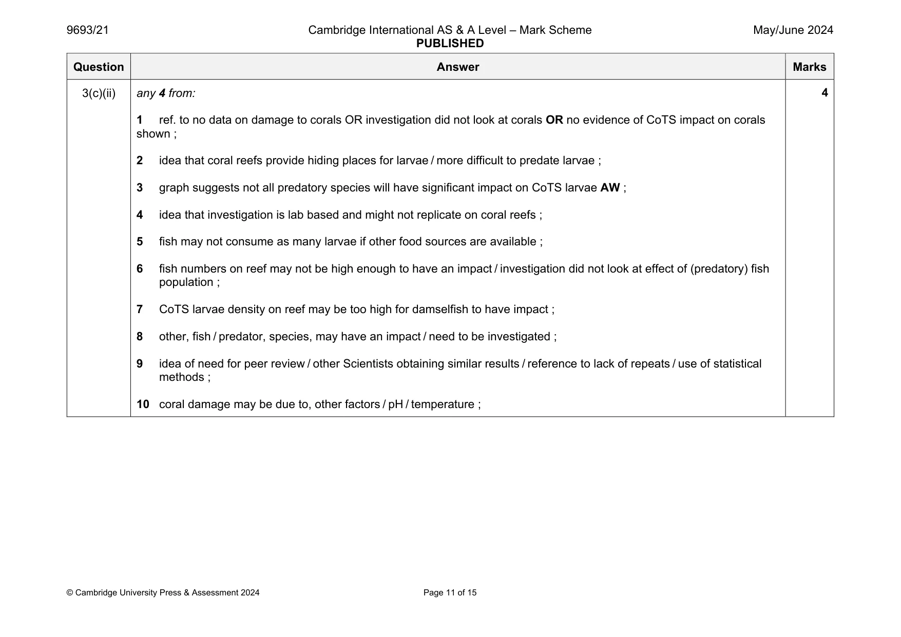
Mark scheme: 3(a) correct labels for both axes and units for x-axis ; correct scale added to both axes ; all plots correct 1 mm / ½ small square ; appropriate line of best fit ; 4 3(b) any 3 from ; idea that both have positive relationship ; idea that rate of increase, levels off / plateaus, for both ; idea that predation by damselfish is (always) greater OR rate of increase in damselfish is greater ; correct use of manipulated data to support comparison ; 3 Question Answer Marks 3(c)(i) any 2 from ; (fewer predatory fish will lead to) decreased predation of (CoTS) larvae OR increased abundance / overpopulation, of (CoTS) larvae ; Idea of more larvae will become, adults / starfish ; ref. to increased population of CoTS feeding on coral ; idea of less predation of other coral consuming organisms if predators removed / predatory fish eat the fish that feed on the corals / prey of these predators that use coral overpopulate, could damage corals / removal of predatory fish damages the coral because there is no hunting of invasive species which eat coral ; AVP ; 2 Question Answer Marks 3(c)(ii) any 4 from: 1 ref. to no data on damage to corals OR investigation did not look at corals OR no evidence of CoTS impact on corals shown ; 2 idea that coral reefs provide hiding places for larvae / more difficult to predate larvae ; 3 graph suggests not all predatory species will have significant impact on CoTS larvae AW ; 4 idea that investigation is lab based and might not replicate on coral reefs ; 5 fish may not consume as many larvae if other food sources are available ; 6 fish numbers on reef may not be high enough to have an impact / investigation did not look at effect of (predatory) fish population ; 7 CoTS larvae density on reef may be too high for damselfish to have impact ; 8 other, fish / predator, species, may have an impact / need to be investigated ; 9 idea of need for peer review / other Scientists obtaining similar results / reference to lack of repeats / use of statistical methods ; 10 coral damage may be due to, other factors / pH / temperature ; 4
Q4 · Lugworms are a species of worm found on sandy and muddy shores
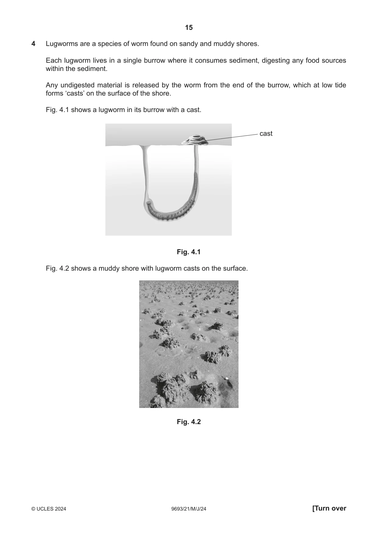
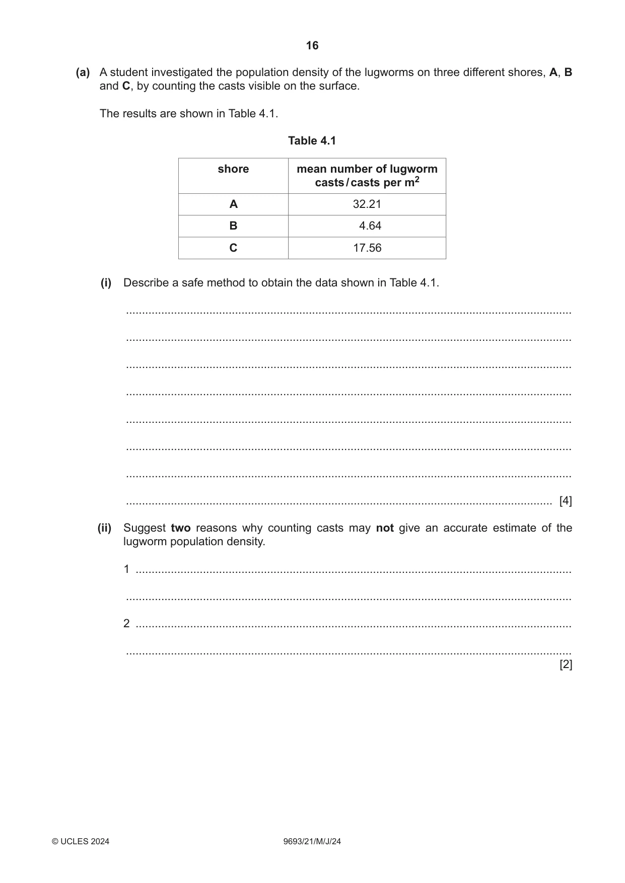
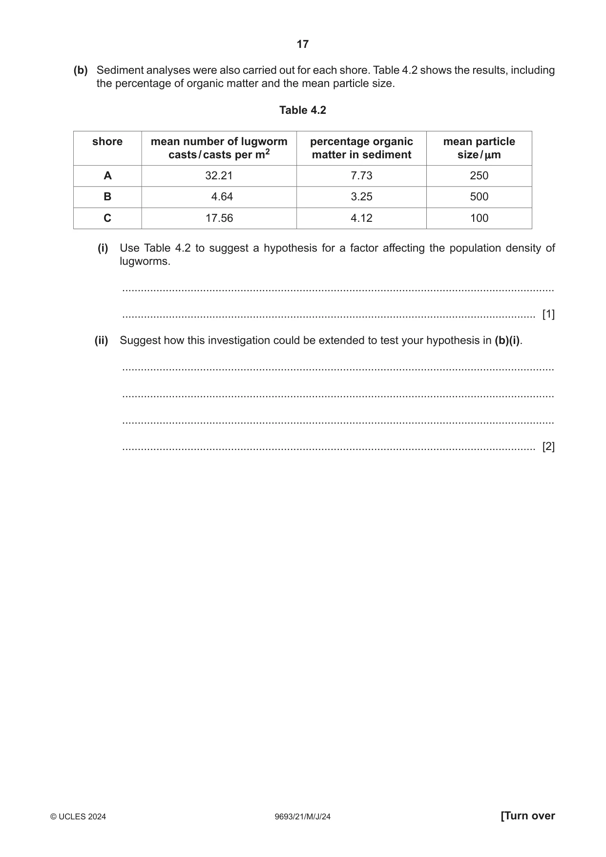
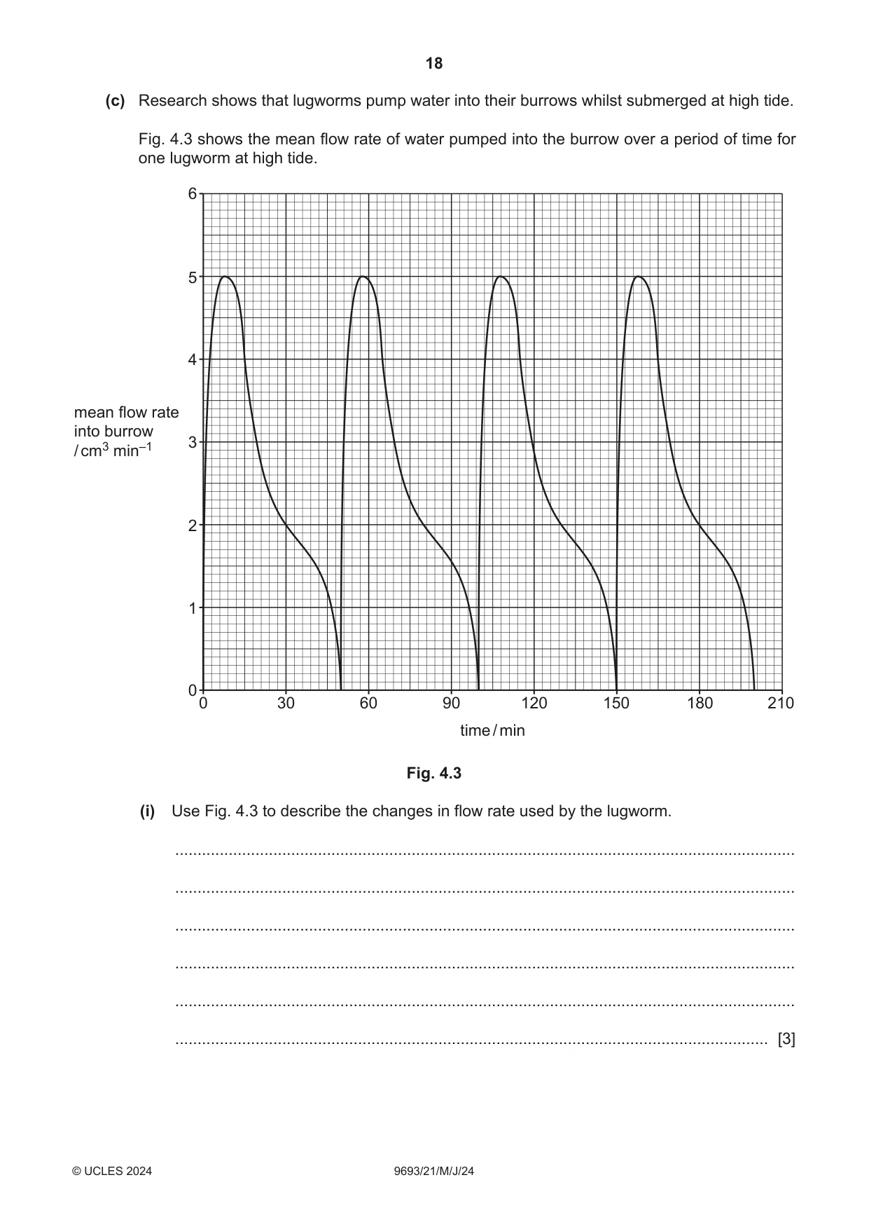
4 Lugworms are a species of worm found on sandy and muddy shores. Each lugworm lives in a single burrow where it consumes sediment, digesting any food sources within the sediment. Any undigested material is released by the worm from the end of the burrow, which at low tide forms ‘casts’ on the surface of the shore. Fig. 4.1 shows a lugworm in its burrow with a cast. cast Fig. 4.1 Fig. 4.2 shows a muddy shore with lugworm casts on the surface. Fig. 4.2 (a) A student investigated the population density of the lugworms on three different shores, A, B and C, by counting the casts visible on the surface. The results are shown in Table 4.1. Table 4.1 shore mean number of lugworm casts / casts per m2 A 32.21 B 4.64 C 17.56 (i) Describe a safe method to obtain the data shown in Table 4.1. ........................................................................................................................................... ........................................................................................................................................... ........................................................................................................................................... ........................................................................................................................................... ........................................................................................................................................... ........................................................................................................................................... ........................................................................................................................................... ..................................................................................................................................... [4] (ii) Suggest two reasons why counting casts may not give an accurate estimate of the lugworm population density. 1 ........................................................................................................................................ ........................................................................................................................................... 2 ........................................................................................................................................ ........................................................................................................................................... [2] (b) Sediment analyses were also carried out for each shore. Table 4.2 shows the results, including the percentage of organic matter and the mean particle size. Table 4.2 shore mean number of lugworm percentage organic mean particle casts / casts per m2 matter in sediment size / μm A 32.21 7.73 250 B 4.64 3.25 500 C 17.56 4.12 100 (i) Use Table 4.2 to suggest a hypothesis for a factor affecting the population density of lugworms. ........................................................................................................................................... ..................................................................................................................................... [1] (ii) Suggest how this investigation could be extended to test your hypothesis in (b)(i). ........................................................................................................................................... ........................................................................................................................................... ........................................................................................................................................... ..................................................................................................................................... [2] (c) Research shows that lugworms pump water into their burrows whilst submerged at high tide. Fig. 4.3 shows the mean flow rate of water pumped into the burrow over a period of time for one lugworm at high tide. 6 5 4 mean flow rate into burrow 3/ cm3 min–1 2 1 0 0 30 60 90 120 150 180 210 time / min Fig. 4.3 (i) Use Fig. 4.3 to describe the changes in flow rate used by the lugworm. ........................................................................................................................................... ........................................................................................................................................... ........................................................................................................................................... ........................................................................................................................................... ........................................................................................................................................... ..................................................................................................................................... [3] (ii) Suggest advantages for the lugworm of pumping water into its burrow. ........................................................................................................................................... ........................................................................................................................................... ........................................................................................................................................... ........................................................................................................................................... ........................................................................................................................................... ..................................................................................................................................... [3] [Total: 15]
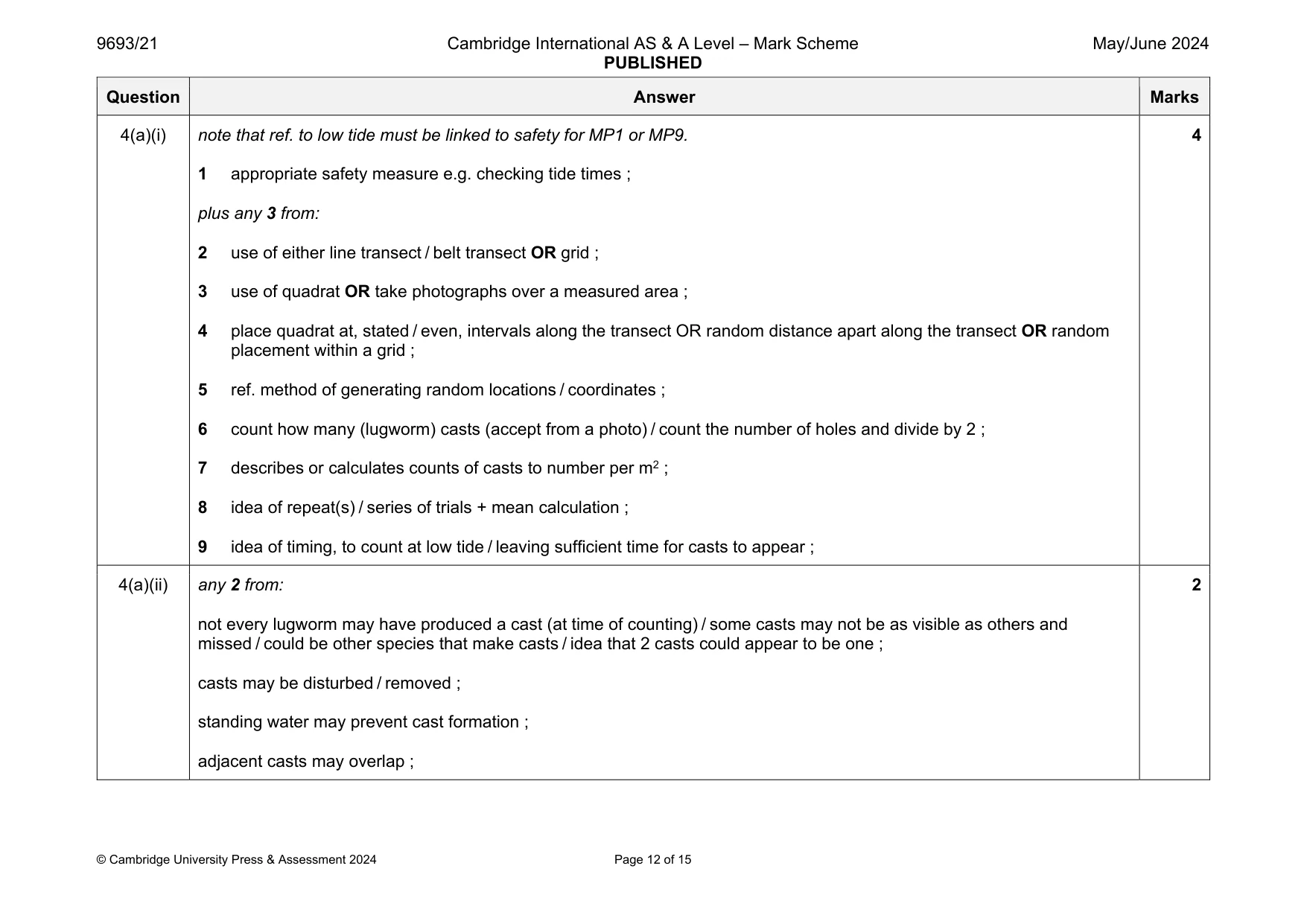
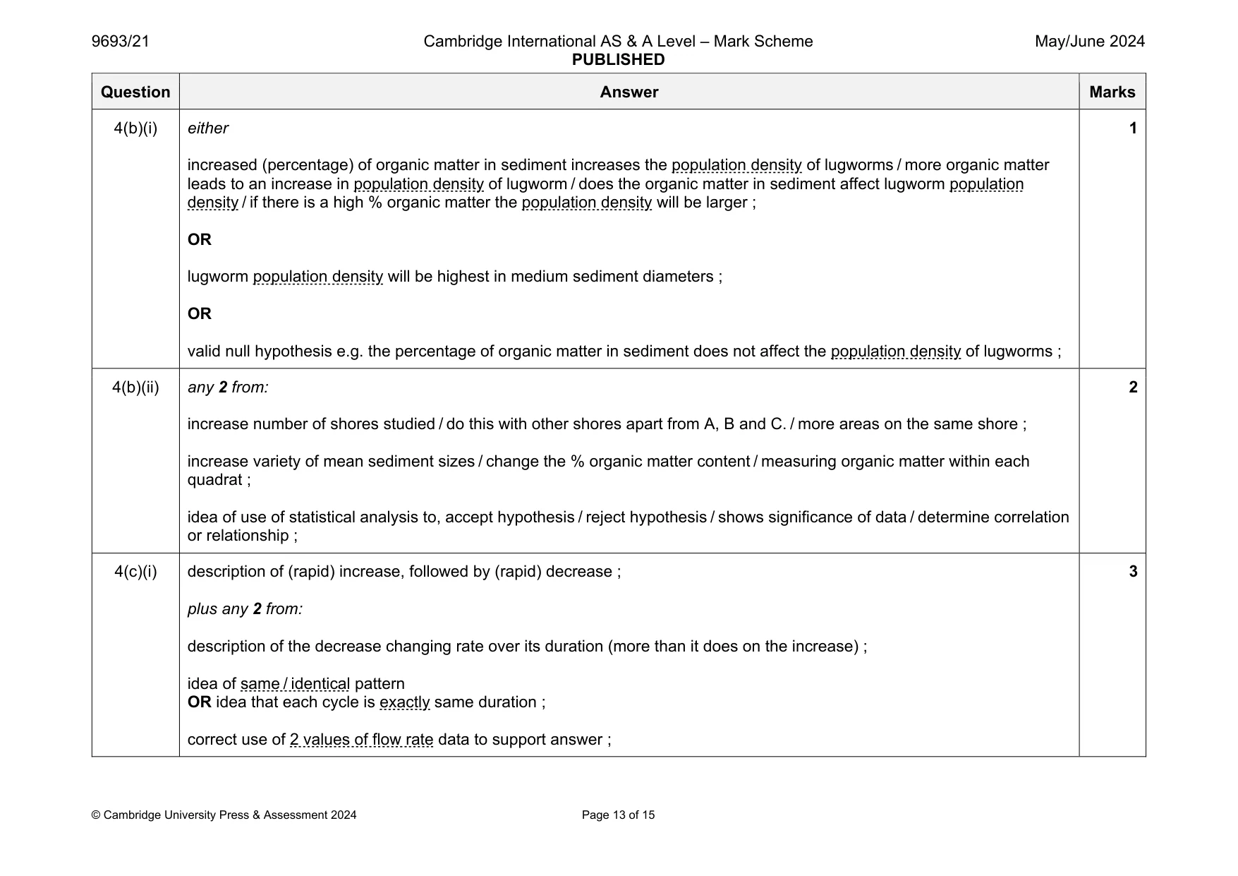
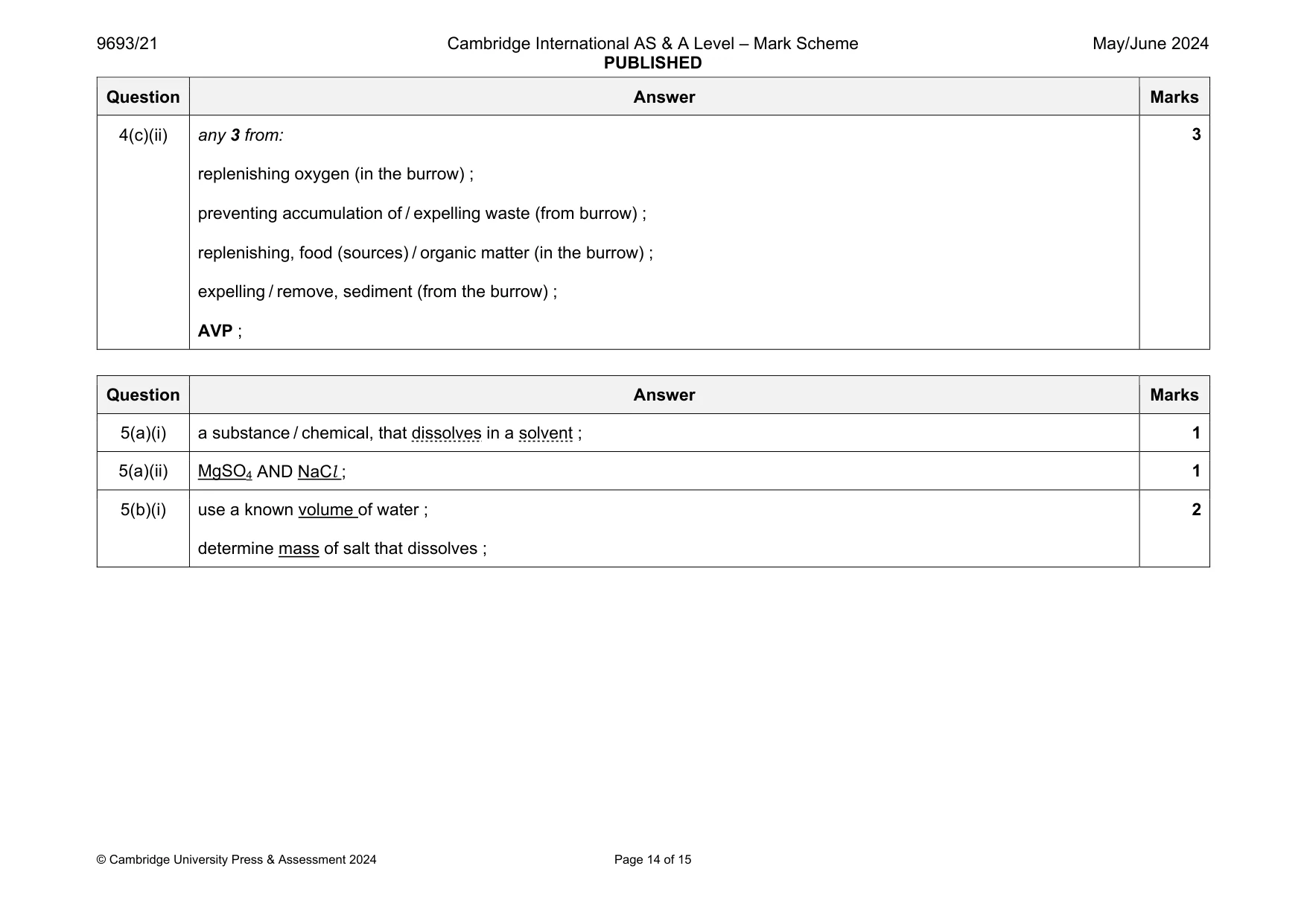
Mark scheme: 4(a)(i) note that ref. to low tide must be linked to safety for MP1 or MP9. 1 appropriate safety measure e.g. checking tide times ; plus any 3 from: 2 use of either line transect / belt transect OR grid ; 3 use of quadrat OR take photographs over a measured area ; 4 place quadrat at, stated / even, intervals along the transect OR random distance apart along the transect OR random placement within a grid ; 5 ref. method of generating random locations / coordinates ; 6 count how many (lugworm) casts (accept from a photo) / count the number of holes and divide by 2 ; 7 describes or calculates counts of casts to number per m2 ; 8 idea of repeat(s) / series of trials + mean calculation ; 9 idea of timing, to count at low tide / leaving sufficient time for casts to appear ; 4 4(a)(ii) any 2 from: not every lugworm may have produced a cast (at time of counting) / some casts may not be as visible as others and missed / could be other species that make casts / idea that 2 casts could appear to be one ; casts may be disturbed / removed ; standing water may prevent cast formation ; adjacent casts may overlap ; 2 Question Answer Marks 4(b)(i) either increased (percentage) of organic matter in sediment increases the population density of lugworms / more organic matter leads to an increase in population density of lugworm / does the organic matter in sediment affect lugworm population density / if there is a high % organic matter the population density will be larger ; OR lugworm population density will be highest in medium sediment diameters ; OR valid null hypothesis e.g. the percentage of organic matter in sediment does not affect the population density of lugworms ; 1 4(b)(ii) any 2 from: increase number of shores studied / do this with other shores apart from A, B and C. / more areas on the same shore ; increase variety of mean sediment sizes / change the % organic matter content / measuring organic matter within each quadrat ; idea of use of statistical analysis to, accept hypothesis / reject hypothesis / shows significance of data / determine correlation or relationship ; 2 4(c)(i) description of (rapid) increase, followed by (rapid) decrease ; plus any 2 from: description of the decrease changing rate over its duration (more than it does on the increase) ; idea of same / identical pattern OR idea that each cycle is exactly same duration ; correct use of 2 values of flow rate data to support answer ; 3 Question Answer Marks 4(c)(ii) any 3 from: replenishing oxygen (in the burrow) ; preventing accumulation of / expelling waste (from burrow) ; replenishing, food (sources) / organic matter (in the burrow) ; expelling / remove, sediment (from the burrow) ; AVP ; 3
Q5 · Magnesium sulfate and sodium chloride are examples of solutes
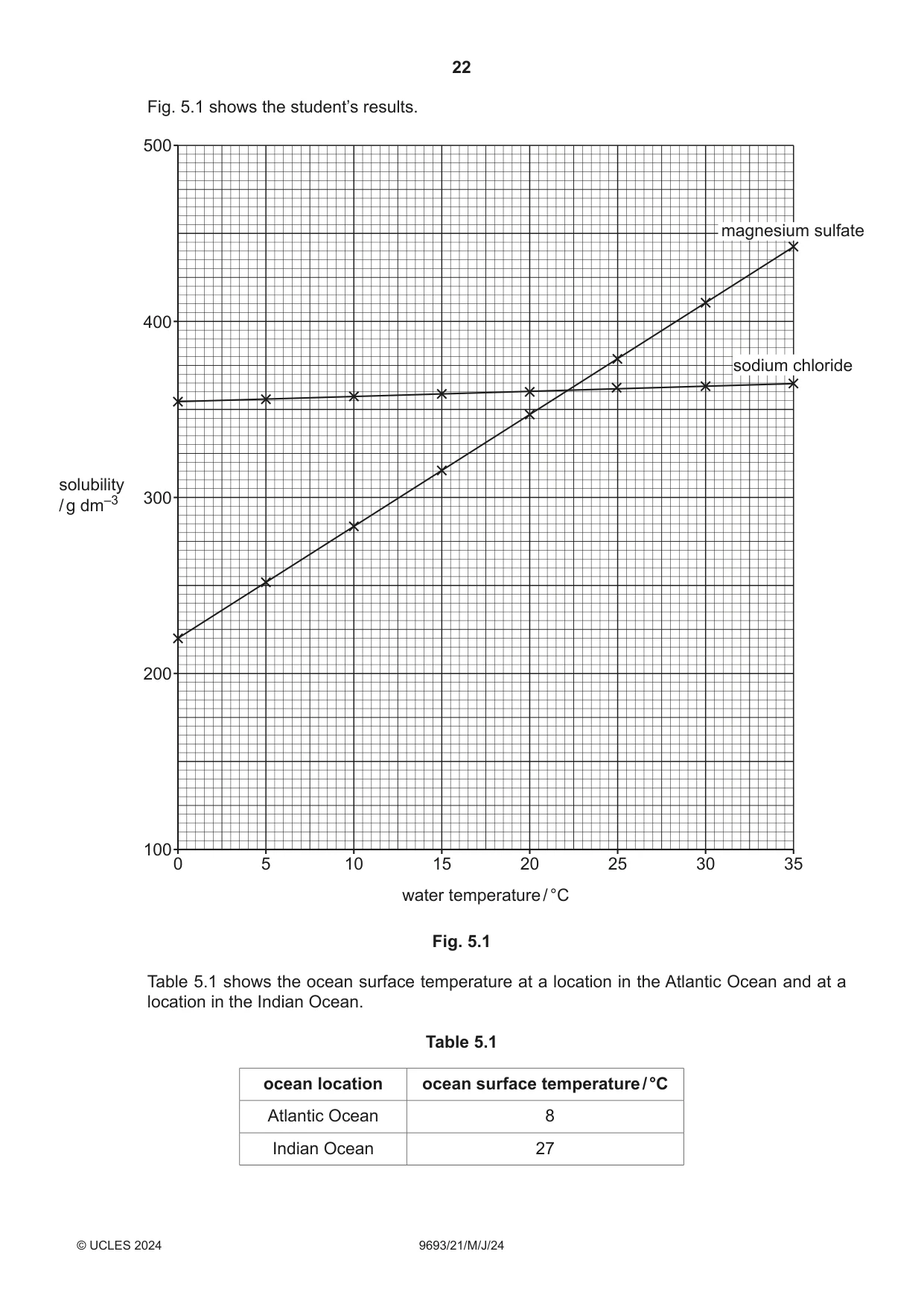
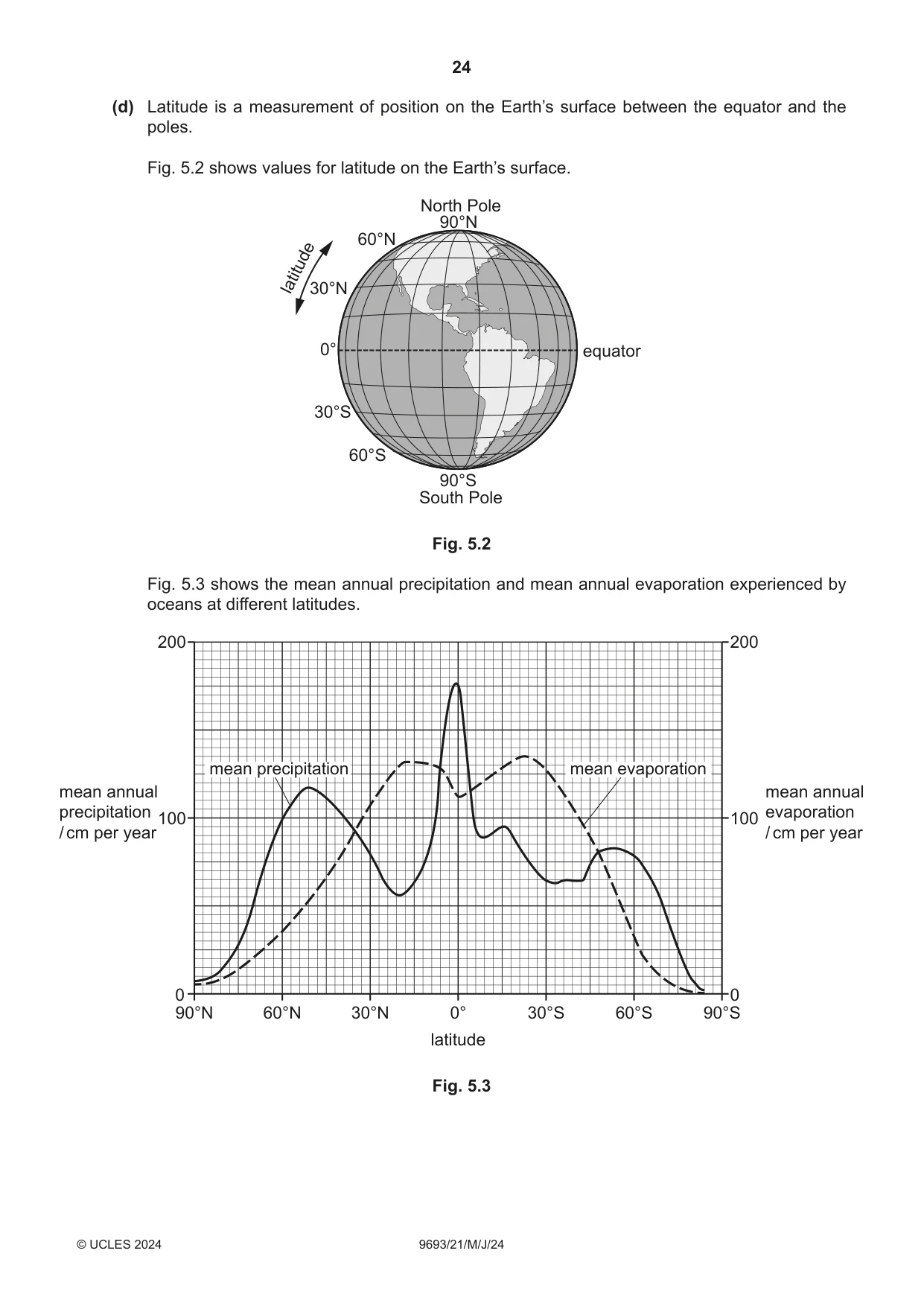
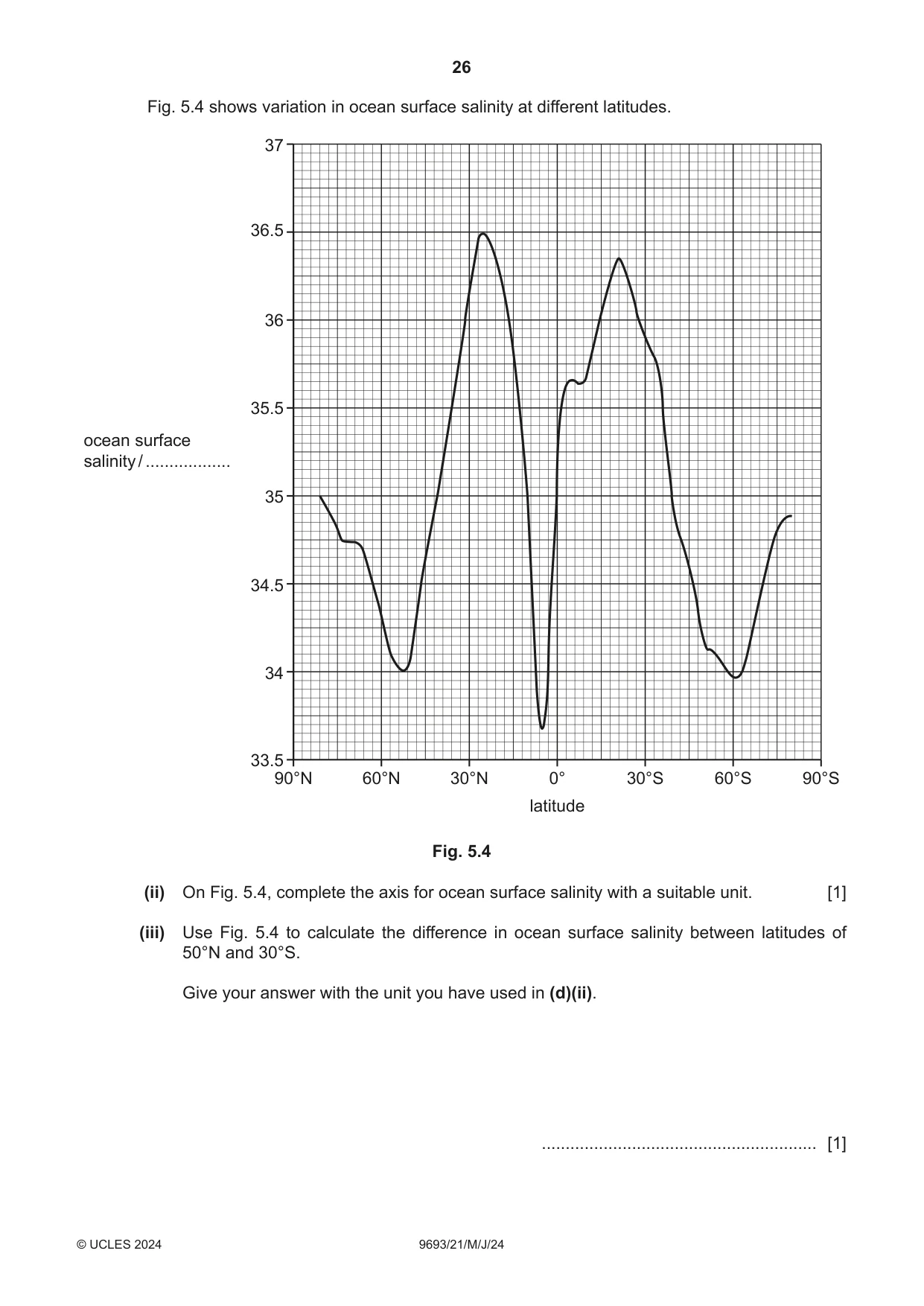
5 (a) Magnesium sulfate and sodium chloride are examples of solutes. (i) Define the term solute. ........................................................................................................................................... ..................................................................................................................................... [1] (ii) State the chemical formulae for magnesium sulfate and sodium chloride. magnesium sulfate ............................................................................................................ sodium chloride ................................................................................................................. [1] A student investigated the solubility of magnesium sulfate and sodium chloride in water at different temperatures. (b) (i) Describe how the student could determine the solubility of each salt in water. ........................................................................................................................................... ........................................................................................................................................... ........................................................................................................................................... ..................................................................................................................................... [2] Fig. 5.1 shows the student’s results. 500 magnesium sulfate 400 sodium chloride solubility 300/ g dm–3 200 100 0 5 10 15 20 25 30 35 water temperature / °C Fig. 5.1 Table 5.1 shows the ocean surface temperature at a location in the Atlantic Ocean and at a location in the Indian Ocean. Table 5.1 ocean location ocean surface temperature / °C Atlantic Ocean 8 Indian Ocean 27 (ii) Use the results in Fig. 5.1 and the information in Table 5.1 to compare the solubilities of magnesium sulfate and sodium chloride at the two ocean locations. ........................................................................................................................................... ........................................................................................................................................... ........................................................................................................................................... ........................................................................................................................................... ........................................................................................................................................... ..................................................................................................................................... [3] (c) Hydrothermal vents are usually found along plate boundaries close to mid-ocean ridges. (i) State the type of plate boundary found at mid-ocean ridges. ..................................................................................................................................... [1] The water coming out of these hydrothermal vents is usually under pressure, at a high temperature and contains a high concentration of dissolved salts. (ii) Explain how chimneys form at hydrothermal vents. Use the trends shown in Fig. 5.1 and your own knowledge in your answer. ........................................................................................................................................... ........................................................................................................................................... ........................................................................................................................................... ........................................................................................................................................... ........................................................................................................................................... ..................................................................................................................................... [3]
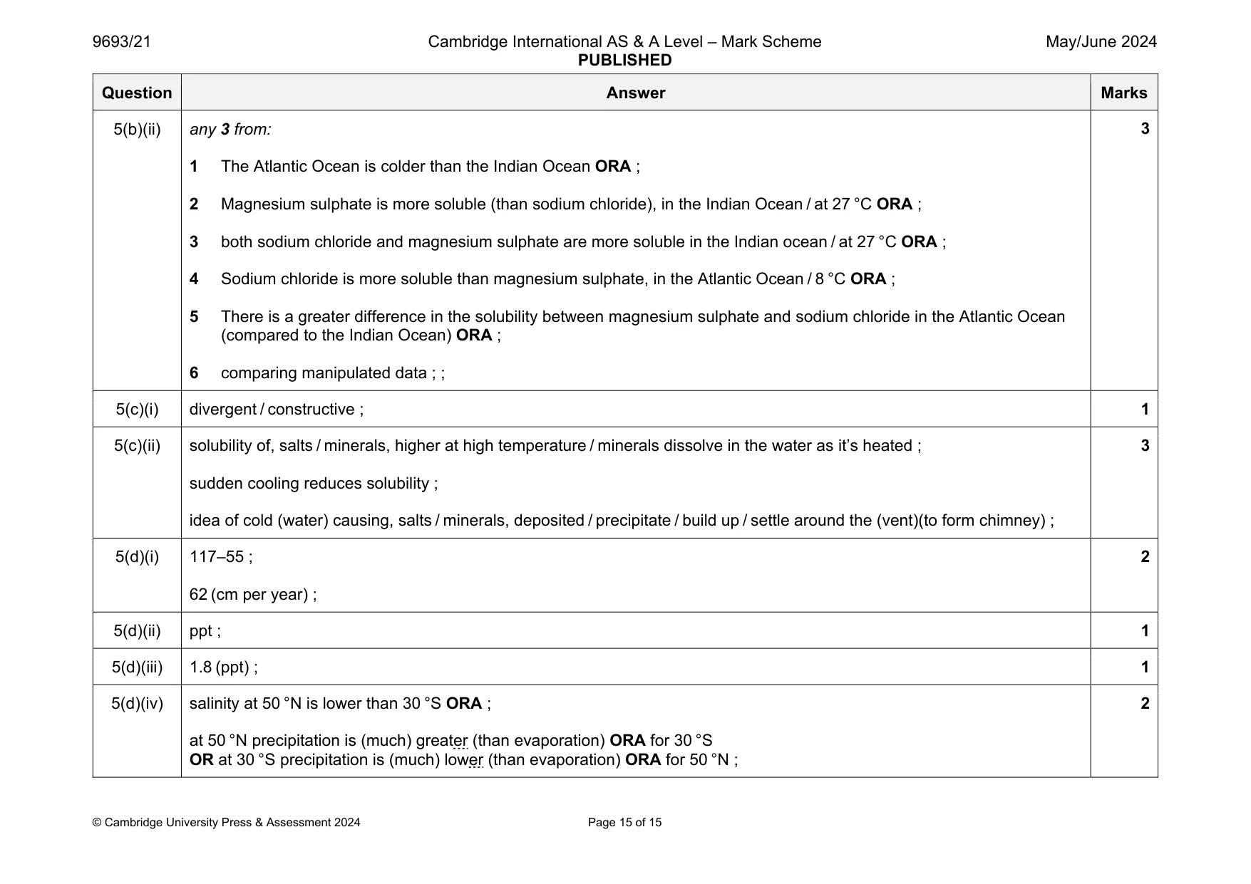
Mark scheme: 5(a)(i) a substance / chemical, that dissolves in a solvent ; 1 5(a)(ii) MgSO4 AND NaCl ; 1 5(b)(i) use a known volume of water ; determine mass of salt that dissolves ; 2 Question Answer Marks 5(b)(ii) any 3 from: 1 The Atlantic Ocean is colder than the Indian Ocean ORA ; 2 Magnesium sulphate is more soluble (than sodium chloride), in the Indian Ocean / at 27 °C ORA ; 3 both sodium chloride and magnesium sulphate are more soluble in the Indian ocean / at 27 °C ORA ; 4 Sodium chloride is more soluble than magnesium sulphate, in the Atlantic Ocean / 8 °C ORA ; 5 There is a greater difference in the solubility between magnesium sulphate and sodium chloride in the Atlantic Ocean (compared to the Indian Ocean) ORA ; 6 comparing manipulated data ; ; 3 5(c)(i) divergent / constructive ; 1 5(c)(ii) solubility of, salts / minerals, higher at high temperature / minerals dissolve in the water as it’s heated ; sudden cooling reduces solubility ; idea of cold (water) causing, salts / minerals, deposited / precipitate / build up / settle around the (vent)(to form chimney) ; 3 5(d)(i) 117–55 ; 62 (cm per year) ; 2 5(d)(ii) ppt ; 1 5(d)(iii) 1.8 (ppt) ; 1 5(d)(iv) salinity at 50 °N is lower than 30 °S ORA ; at 50 °N precipitation is (much) greater (than evaporation) ORA for 30 °S OR at 30 °S precipitation is (much) lower (than evaporation) ORA for 50 °N ; 2
What was in this paper
The subtopics covered by these 5 questions, and how many questions each got. Open one in a new tab to see every Cambridge question on it.
What you needed in this session
Cambridge’s own grade thresholds for 2024 May/June, Paper 2 · Variant 1. A higher threshold means an easier paper — the bar moves with how the cohort did.