Questions as text
Q1 · The reactance Xc of a capacitor is defined as For Examiner’s = V0 Xc Use I0 where V0 is… 9702/51 May/June 2010
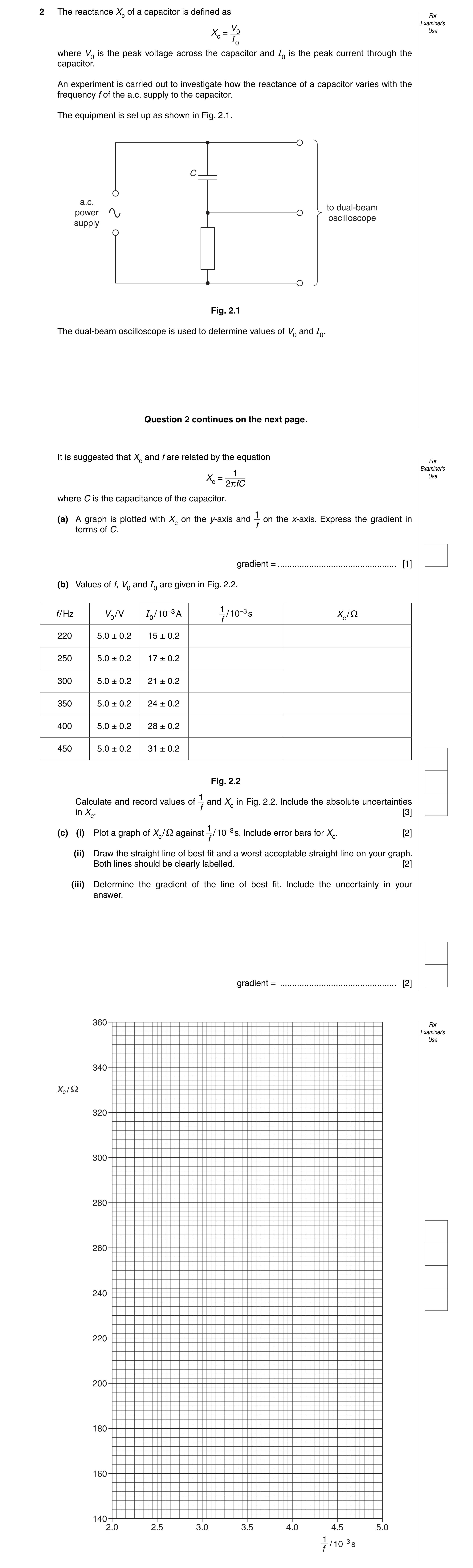
2 The reactance Xc of a capacitor is defined as For Examiner’s = V0 Xc Use I0 where V0 is the peak voltage across the capacitor and I0 is the peak current through the capacitor. An experiment is carried out to investigate how the reactance of a capacitor varies with the frequency f of the a.c. supply to the capacitor. The equipment is set up as shown in Fig. 2.1. C a.c. to dual-beam power oscilloscope supply Fig. 2.1 The dual-beam oscilloscope is used to determine values of V0 and I0. Question 2 continues on the next page. It is suggested that Xc and f are related by the equation For Examiner’s 1 Use Xc = 2 fC where C is the capacitance of the capacitor. 1 (a) A graph is plotted with Xc on the y-axis and on the x-axis. Express the gradient in f terms of C. gradient = … [1] (b) Values of f, V0 and I0 are given in Fig. 2.2. 1 f / Hz V0 / V I0 / 10–3 A / 10–3 s Xc / f 220 5.0 ± 0.2 15 ± 0.2 250 5.0 ± 0.2 17 ± 0.2 300 5.0 ± 0.2 21 ± 0.2 350 5.0 ± 0.2 24 ± 0.2 400 5.0 ± 0.2 28 ± 0.2 450 5.0 ± 0.2 31 ± 0.2 Fig. 2.2 1 Calculate and record values of and Xc in Fig. 2.2. Include the absolute uncertainties f in Xc. [3] 1 (c) (i) Plot a graph of Xc / against / 10–3 s. Include error bars for Xc. [2] f (ii) Draw the straight line of best fit and a worst acceptable straight line on your graph. Both lines should be clearly labelled. [2] (iii) Determine the gradient of the line of best fit. Include the uncertainty in your answer. gradient = … [2] 360 For Examiner’s Use 340 Xc / Ω 320 300 280 260 240 220 200 180 160 140 2.0 2.5 3.0 3.5 4.0 4.5 5.0 1 / 10–3 s f
10 marks
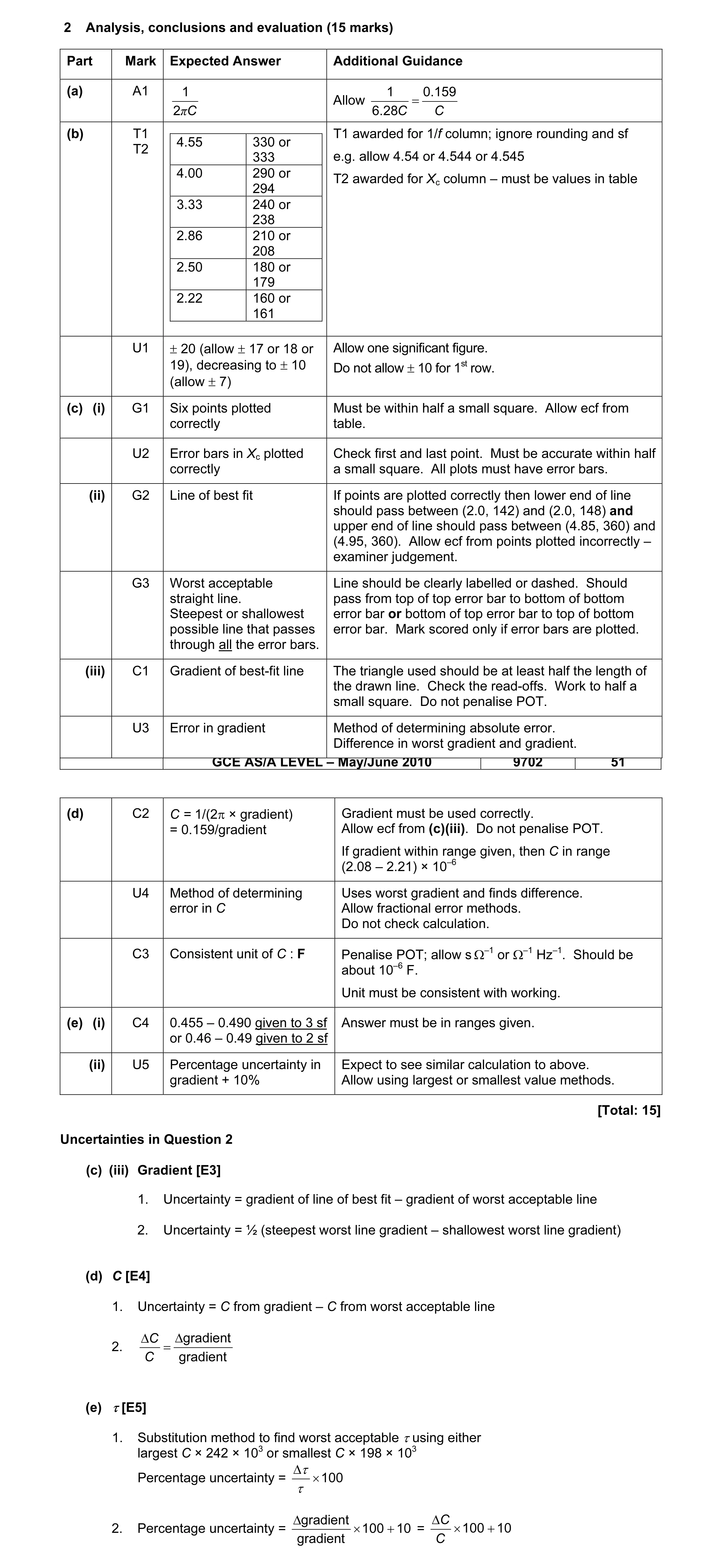
Mark scheme: 2 Analysis, conclusions and evaluation (15 marks) Part Mark Expected Answer Additional Guidance (a) A1 1 1 0.159 Allow = 2πC 6.28C C (b) T1 T1 awarded for 1/f column; ignore rounding and sf 4.55 330 or T2 333 e.g. allow 4.54 or 4.544 or 4.545 4.00 290 or T2 awarded for Xc column – must be values in table 294 3.33 240 or 238 2.86 210 or 208 2.50 180 or 179 2.22 160 or 161 U1 ± 20 (allow ± 17 or 18 or Allow one significant figure. 19), decreasing to ± 10 Do not allow ± 10 for 1st row. (allow ± 7) (c) (i) G1 Six points plotted Must be within half a small square. Allow ecf from correctly table. U2 Error bars in Xc plotted Check first and last point. Must be accurate within half correctly a small square. All plots must have error bars. (ii) G2 Line of best fit If points are plotted correctly then lower end of line should pass between (2.0, 142) and (2.0, 148) and upper end of line should pass between (4.85, 360) and (4.95, 360). Allow ecf from points plotted incorrectly – examiner judgement. G3 Worst acceptable Line should be clearly labelled or dashed. Should straight line. pass from top of top error bar to bottom of bottom Steepest or shallowest error bar or bottom of top error bar to top of bottom possible line that passes error bar. Mark scored only if error bars are plotted. through all the error bars. (iii) C1 Gradient of best-fit line The triangle used should be at least half the length of the drawn line. Check the read-offs. Work to half a small square. Do not penalise POT. U3 Error in gradient Method of determining absolute error. Difference in worst gradient and gradient. GCE AS/A LEVEL – May/June 2010 9702 51 (d) C2 C = 1/(2π × gradient) Gradient must be used correctly. = 0.159/gradient Allow ecf from (c)(iii). Do not penalise POT. If gradient within range given, then C in range (2.08 – 2.21) × 10–6 U4 Method of determining Uses worst gradient and finds difference. error in C Allow fractional error methods. Do not check calculation. C3 Consistent unit of C : F Penalise POT; allow s Ω–1 or Ω–1 Hz–1. Should be about 10–6 F. Unit must be consistent with working. (e) (i) C4 0.455 – 0.490 given to 3 sf Answer must be in ranges given. or 0.46 – 0.49 given to 2 sf (ii) U5 Percentage uncertainty in Expect to see similar calculation to above. gradient + 10% Allow using largest or smallest value methods. [Total: 15] Uncertainties in Question 2 (c) (iii) Gradient [E3] 1. Uncertainty = gradient of line of best fit – gradient of worst acceptable line 2. Uncertainty = ½ (steepest worst line gradient – shallowest worst line gradient) (d) C [E4] 1. Uncertainty = C from gradient – C from worst acceptable line ∆C ∆gradient 2. = C gradient (e) τ [E5] 1. Substitution method to find worst acceptable τ using either largest C × 242 × 103 or smallest C × 198 × 103 ∆τ Percentage uncertainty = × 100 τ ∆gradient ∆C 2. Percentage uncertainty = × 100 + 10 = × 100 + 10 gradient C
This question in 9702/51 May/June 2010
Q2 · A student is investigating the discharge of capacitors 9702/51 May/June 2013
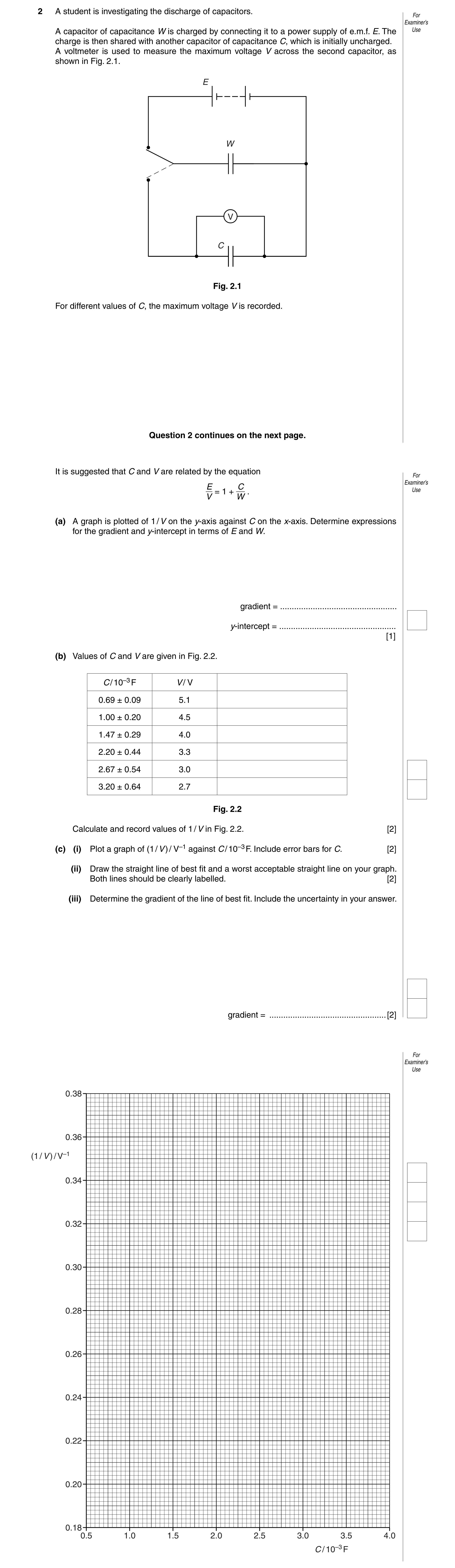
2 A student is investigating the discharge of capacitors. For Examiner’s A capacitor of capacitance W is charged by connecting it to a power supply of e.m.f. E. The Use charge is then shared with another capacitor of capacitance C, which is initially uncharged. A voltmeter is used to measure the maximum voltage V across the second capacitor, as shown in Fig. 2.1. E W V C Fig. 2.1 For different values of C, the maximum voltage V is recorded. Question 2 continues on the next page. It is suggested that C and V are related by the equation For Examiner’s E C Use = 1 + . V W (a) A graph is plotted of 1 / V on the y-axis against C on the x-axis. Determine expressions for the gradient and y-intercept in terms of E and W. gradient = … y-intercept = … [1] (b) Values of C and V are given in Fig. 2.2. C / 10–3 F V / V 0.69 ± 0.09 5.1 1.00 ± 0.20 4.5 1.47 ± 0.29 4.0 2.20 ± 0.44 3.3 2.67 ± 0.54 3.0 3.20 ± 0.64 2.7 Fig. 2.2 Calculate and record values of 1 / V in Fig. 2.2. [2] (c) (i) Plot a graph of (1 / V ) / V–1 against C / 10–3 F. Include error bars for C. [2] (ii) Draw the straight line of best fit and a worst acceptable straight line on your graph. Both lines should be clearly labelled. [2] (iii) Determine the gradient of the line of best fit. Include the uncertainty in your answer. gradient = … [2] For Examiner’s Use 0.38 0.36 (1 / V ) / V–1 0.34 0.32 0.30 0.28 0.26 0.24 0.22 0.20 0.18 0.5 1.0 1.5 2.0 2.5 3.0 3.5 4.0 C / 10–3 F
9 marks
Mark scheme: 2 Analysis, conclusions and evaluation (15 marks) Mark Expected Answer Additional Guidance (a) A1 Gradient = 1 / EW y-intercept = 1 / E (b) T1 1 Column heading. Allow equivalent unit. / V–1 e.g. V–1 / V–1 or 1/V / 1/V or 1/V (V–1) V A mixture of 2 s.f. and 3 s.f. is allowed. T2 0.20 or 0.196 0.22 or 0.222 0.25 or 0.250 0.30 or 0.303 0.33 or 0.333 0.37 or 0.370 (c) (i) G1 Six points plotted correctly Must be less than half a small square. Ecf allowed from table. Penalise ‘blobs’. U1 All error bars in C plotted Must be within half a small square. Ecf allowed correctly from table. Horizontal. (c) (ii) G2 Line of best fit If points are plotted correctly then lower end of line should pass between (0.75, 0.200) and (0.75, 0.205) and upper end of line should pass between (3.0, 0.352) and (3.0, 0.358). Allow ecf from points plotted incorrectly – examiner judgement. G3 Worst acceptable straight Line should be clearly labelled or dashed. Should line. pass from top of top error bar to bottom of bottom Steepest or shallowest error bar or bottom of top error bar to top of bottom possible line that passes error bar. Mark scored only if error bars are plotted. through all the error bars. (c) (iii) C1 Gradient of best fit line The triangle used should be at least half the length of the drawn line. Check the read offs. Work to half a small square. Do not penalise POT. U2 Uncertainty in gradient Method of determining absolute uncertainty Difference in worst gradient and gradient. (c) (iv) C2 y-intercept Expect to see point substituted into y = mx + c FOX does not score. Do not penalise POT. Should be about 0.15. U3 Uncertainty in y-intercept Difference in worst y-intercept and y-intercept. FOX does not score. Allow ecf from (c)(iv). GCE AS/A LEVEL – May/June 2013 9702 51 (d) (i) C3 E = 1/ y-intercept and V Method required. Do not check calculation. Allow ecf from (c)(iv). U4 Absolute uncertainty in E (d) (ii) C4 Between 2.00 × 10⁻³ F and Must be in range. Allow use of mF. 2.40 × 10⁻³ F and given to 2 or 3 s.f. (d) (iii) U5 Percentage uncertainty in W %uncertainty in E + %uncertainty in gradient [Total: 15] Uncertainties in Question 2 (c) (iii) Gradient [U2] Uncertainty = gradient of line of best fit – gradient of worst acceptable line Uncertainty = ½ (steepest worst line gradient – shallowest worst line gradient) (c) (iv) y-intercept [U3] Uncertainty = y-intercept of line of best fit – y-intercept of worst acceptable line Uncertainty = ½ (steepest worst line y-intercept – shallowest worst line y-intercept) (d) (i) [U4] max E − min E Absolute uncertainty = max E – E = E – min E = 2 ∆c Absolute uncertainty = × E c (d) (iii) [U5] ∆W Percentage uncertainty = × 100 W max W − min W ∆W = max W – W = W – min W = 2 1 max W = min E × min m 1 min W= max E × max m ∆m ∆E ∆ m ∆ c Percentage uncertainty = + × 100 = + × 100 m E m c
This question in 9702/51 May/June 2013
Q3 · A student is investigating the discharge of capacitors 9702/53 May/June 2013
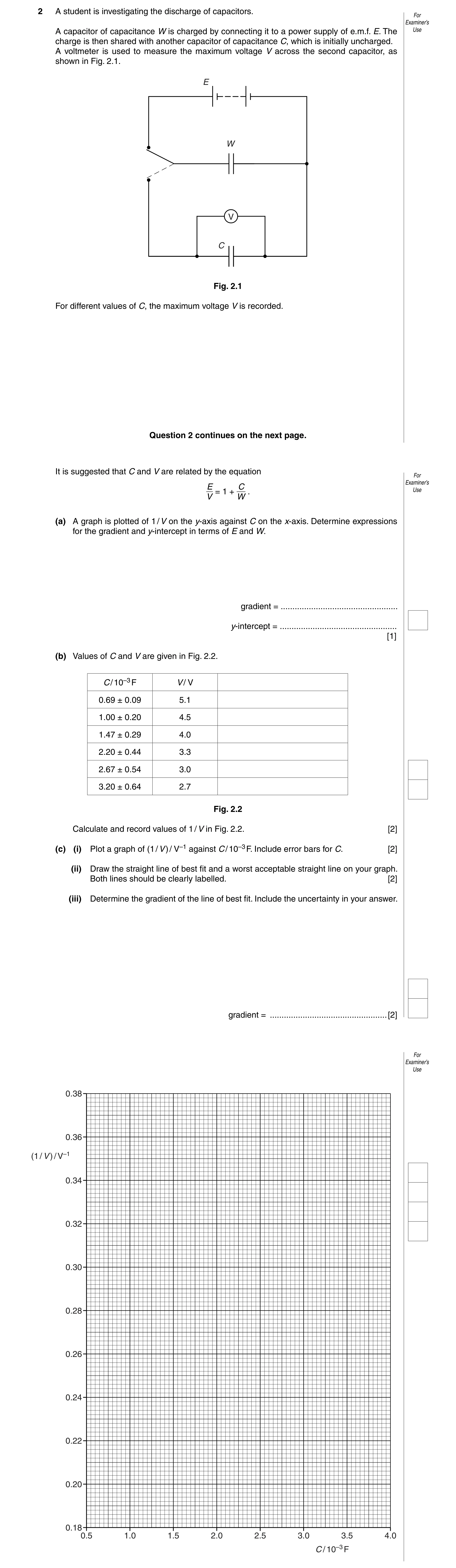
2 A student is investigating the discharge of capacitors. For Examiner’s A capacitor of capacitance W is charged by connecting it to a power supply of e.m.f. E. The Use charge is then shared with another capacitor of capacitance C, which is initially uncharged. A voltmeter is used to measure the maximum voltage V across the second capacitor, as shown in Fig. 2.1. E W V C Fig. 2.1 For different values of C, the maximum voltage V is recorded. Question 2 continues on the next page. It is suggested that C and V are related by the equation For Examiner’s E C Use = 1 + . V W (a) A graph is plotted of 1 / V on the y-axis against C on the x-axis. Determine expressions for the gradient and y-intercept in terms of E and W. gradient = … y-intercept = … [1] (b) Values of C and V are given in Fig. 2.2. C / 10–3 F V / V 0.69 ± 0.09 5.1 1.00 ± 0.20 4.5 1.47 ± 0.29 4.0 2.20 ± 0.44 3.3 2.67 ± 0.54 3.0 3.20 ± 0.64 2.7 Fig. 2.2 Calculate and record values of 1 / V in Fig. 2.2. [2] (c) (i) Plot a graph of (1 / V ) / V–1 against C / 10–3 F. Include error bars for C. [2] (ii) Draw the straight line of best fit and a worst acceptable straight line on your graph. Both lines should be clearly labelled. [2] (iii) Determine the gradient of the line of best fit. Include the uncertainty in your answer. gradient = … [2] For Examiner’s Use 0.38 0.36 (1 / V ) / V–1 0.34 0.32 0.30 0.28 0.26 0.24 0.22 0.20 0.18 0.5 1.0 1.5 2.0 2.5 3.0 3.5 4.0 C / 10–3 F
9 marks
Mark scheme: 2 Analysis, conclusions and evaluation (15 marks) Mark Expected Answer Additional Guidance (a) A1 Gradient = 1 / EW y-intercept = 1 / E (b) T1 1 Column heading. Allow equivalent unit. / V–1 e.g. V–1 / V–1 or 1/V / 1/V or 1/V (V–1) V A mixture of 2 s.f. and 3 s.f. is allowed. T2 0.20 or 0.196 0.22 or 0.222 0.25 or 0.250 0.30 or 0.303 0.33 or 0.333 0.37 or 0.370 (c) (i) G1 Six points plotted correctly Must be less than half a small square. Ecf allowed from table. Penalise ‘blobs’. U1 All error bars in C plotted Must be within half a small square. Ecf allowed correctly from table. Horizontal. (c) (ii) G2 Line of best fit If points are plotted correctly then lower end of line should pass between (0.75, 0.200) and (0.75, 0.205) and upper end of line should pass between (3.0, 0.352) and (3.0, 0.358). Allow ecf from points plotted incorrectly – examiner judgement. G3 Worst acceptable straight Line should be clearly labelled or dashed. Should line. pass from top of top error bar to bottom of bottom Steepest or shallowest error bar or bottom of top error bar to top of bottom possible line that passes error bar. Mark scored only if error bars are plotted. through all the error bars. (c) (iii) C1 Gradient of best fit line The triangle used should be at least half the length of the drawn line. Check the read offs. Work to half a small square. Do not penalise POT. U2 Uncertainty in gradient Method of determining absolute uncertainty Difference in worst gradient and gradient. (c) (iv) C2 y-intercept Expect to see point substituted into y = mx + c FOX does not score. Do not penalise POT. Should be about 0.15. U3 Uncertainty in y-intercept Difference in worst y-intercept and y-intercept. FOX does not score. Allow ecf from (c)(iv). GCE AS/A LEVEL – May/June 2013 9702 53 (d) (i) C3 E = 1/ y-intercept and V Method required. Do not check calculation. Allow ecf from (c)(iv). U4 Absolute uncertainty in E (d) (ii) C4 Between 2.00 × 10⁻³ F and Must be in range. Allow use of mF. 2.40 × 10⁻³ F and given to 2 or 3 s.f. (d) (iii) U5 Percentage uncertainty in W %uncertainty in E + %uncertainty in gradient [Total: 15] Uncertainties in Question 2 (c) (iii) Gradient [U2] Uncertainty = gradient of line of best fit – gradient of worst acceptable line Uncertainty = ½ (steepest worst line gradient – shallowest worst line gradient) (c) (iv) y-intercept [U3] Uncertainty = y-intercept of line of best fit – y-intercept of worst acceptable line Uncertainty = ½ (steepest worst line y-intercept – shallowest worst line y-intercept) (d) (i) [U4] max E − min E Absolute uncertainty = max E – E = E – min E = 2 ∆c Absolute uncertainty = × E c (d) (iii) [U5] ∆W Percentage uncertainty = × 100 W max W − min W ∆W = max W – W = W – min W = 2 1 max W = min E × min m 1 min W= max E × max m ∆m ∆E ∆ m ∆ c Percentage uncertainty = + × 100 = + × 100 m E m c
This question in 9702/53 May/June 2013
Q4 · A student investigates electrical resonance in a circuit containing a capacitor and a… 9702/51 Oct/Nov 2014
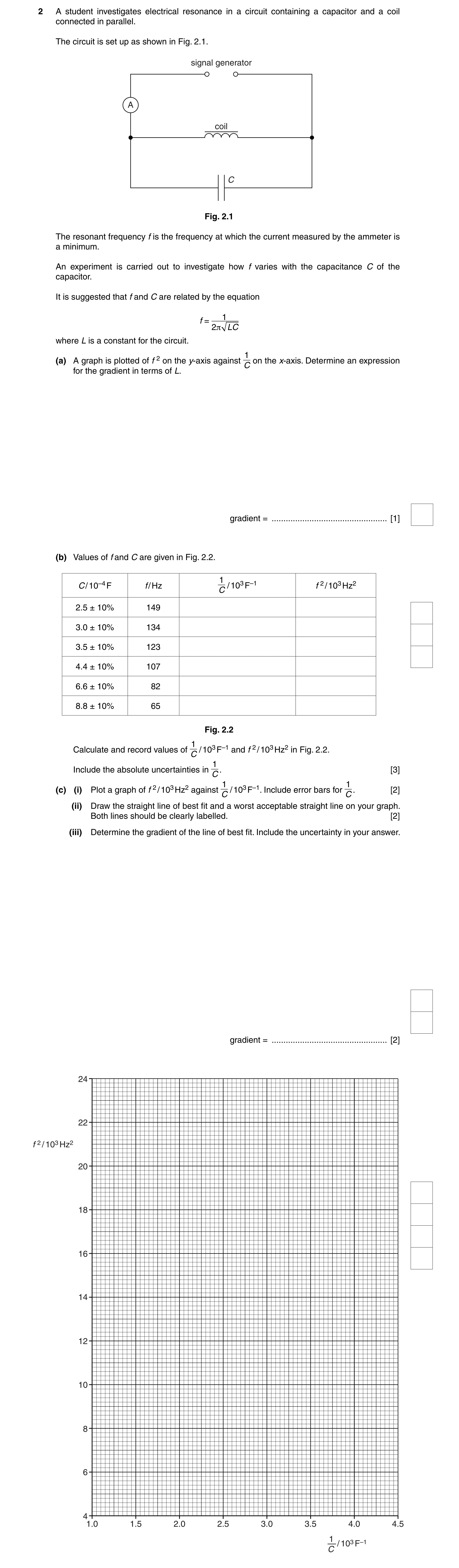
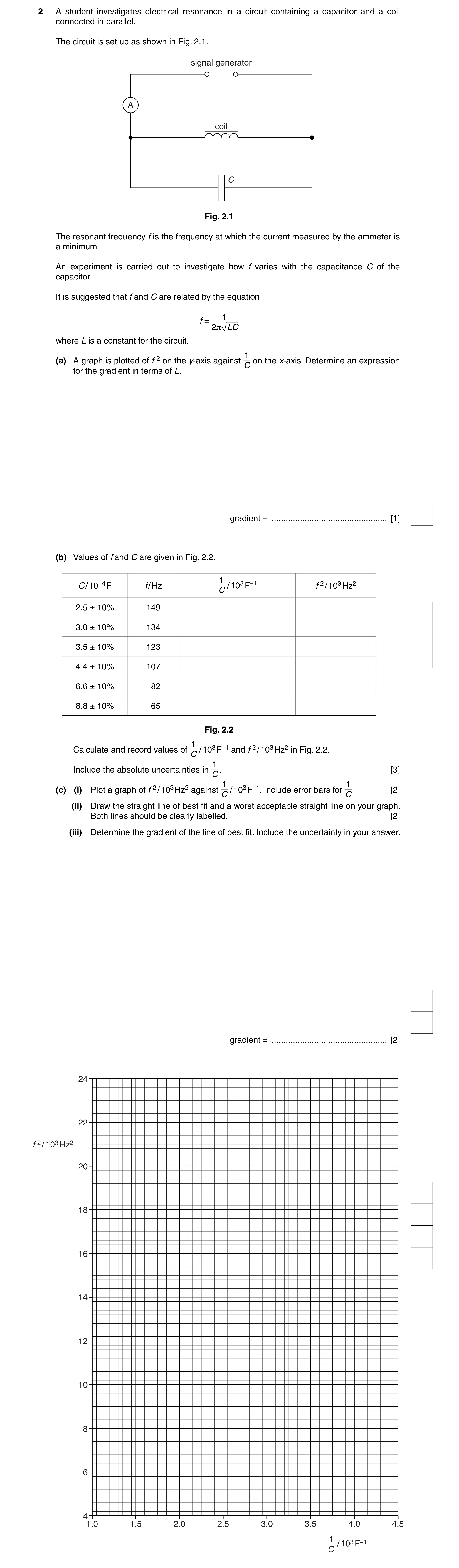
2 A student investigates electrical resonance in a circuit containing a capacitor and a coil connected in parallel. The circuit is set up as shown in Fig. 2.1. signal generator A coil C Fig. 2.1 The resonant frequency f is the frequency at which the current measured by the ammeter is a minimum. An experiment is carried out to investigate how f varies with the capacitance C of the capacitor. It is suggested that f and C are related by the equation 1 f = 2π LC where L is a constant for the circuit. 2 1 (a) A graph is plotted of f on the y-axis against on the x-axis. Determine an expression C for the gradient in terms of L. gradient = … [1] (b) Values of f and C are given in Fig. 2.2. 1 C / 10–4 F f / Hz / 103 F–1 f 2 / 103 Hz2 C 2.5 ± 10% 149 3.0 ± 10% 134 3.5 ± 10% 123 4.4 ± 10% 107 6.6 ± 10% 82 8.8 ± 10% 65 Fig. 2.2 1 2 Calculate and record values of / 103 F–1 and f / 103 Hz2 in Fig. 2.2. C 1 Include the absolute uncertainties in . [3] C 2 1 1(c) (i) Plot a graph of f / 103 Hz2 against / 103 F–1. Include error bars for . [2] C C (ii) Draw the straight line of best fit and a worst acceptable straight line on your graph. Both lines should be clearly labelled. [2] (iii) Determine the gradient of the line of best fit. Include the uncertainty in your answer. gradient = … [2] 24 22 f 2 / 103 Hz2 20 18 16 14 12 10 8 6 4 1.0 1.5 2.0 2.5 3.0 3.5 4.0 4.5 1 — / 103 F–1 C
10 marks
Mark scheme: 2 Analysis, conclusions and evaluation (15 marks) Mark Expected Answer Additional Guidance (a) A1 1 gradient = 2 4 π L (b) T1 T1 (first column) and T2 (second column) T2 4.0 or 4.00 22.2 or 22.20 must be table values. Allow a mixture of significant figures. 3.3 or 3.33 18.0 or 17.96 2.9 or 2.86 15.1 or 15.13 2.3 or 2.27 11.4 or 11.45 1.5 or 1.52 6.7 or 6.72 1.1 or 1.14 4.2 or 4.23 U1 From ± 0.4 (or ± 0.5) to ± 0.1 Allow more than one significant figure. (or ± 0.2) (c) (i) G1 Six points plotted correctly Must be within half a small square. Penalise “blobs”. Ecf allowed from table. U2 Error bars in 1/C plotted correctly All error bars to be plotted. Must be accurate to less than half a small square. (c) (ii) G2 Line of best fit If points are plotted correctly then lower end of line should pass between (1.65, 8.0) and (1.75, 8.0) and upper end of line should pass between (3.95, 22) and (4.05, 22). Allow ecf from points plotted incorrectly – examiner judgement. G3 Worst acceptable straight line. Line should be clearly labelled or dashed. Steepest or shallowest possible Examiner judgement on worst acceptable line that passes through all the line. Lines must cross. Mark scored only if error bars. all error bars are plotted. (c) (iii) C1 Gradient of best fit line The triangle used should be at least half the length of the drawn line. Check the read-offs. Work to half a small square. Do not penalise POT. (Should be about 6.) U3 Uncertainty in gradient correctly Method of determining absolute determined uncertainty: difference in worst gradient and gradient. (d) C2 1 Allow ecf from (c)(iii). L = 2 (Should be about 4 × 10⁻³.) 4 π × gradient C3 F–1 Hz–2 or s2 F–1 Allow H or kg m2 A–2 s–2 or Ω Hz–1 or Ω s. Conventional notation required. U4 Absolute uncertainty in L. (e) (i) C4 f in the range 760 to 800 and 1 gradient given to 2 or 3 s.f. f = = 2 π LC C (ii) U5 Percentage uncertainty in f. ½(Percentage uncertainty in L + Must be greater than 5%. percentage uncertainty in C) [Total: 15] Uncertainties in Question 2 (c) (iii) Gradient [U3] Uncertainty = gradient of line of best fit – gradient of worst acceptable line Uncertainty = ½(steepest worst line gradient – shallowest worst line gradient) (d) [U4] ∆gradient absolute uncertainty in L = × L gradient 1 max L = 2 4 π × min gradient 1 min L = 4 π 2 × max gradient (e) (ii) [U5] 1 ∆L 1 ∆gradient % uncertainty = × 100 + 10 = × 100 + 10 2 L 2 gradient 1 max gradient max f = = 2 π LminCmin min C 1 min gradient min f = = 2 π Lmax Cmax max C
This question in 9702/51 Oct/Nov 2014
Q5 · A student investigates electrical resonance in a circuit containing a capacitor and a… 9702/52 Oct/Nov 2014
2 A student investigates electrical resonance in a circuit containing a capacitor and a coil connected in parallel. The circuit is set up as shown in Fig. 2.1. signal generator A coil C Fig. 2.1 The resonant frequency f is the frequency at which the current measured by the ammeter is a minimum. An experiment is carried out to investigate how f varies with the capacitance C of the capacitor. It is suggested that f and C are related by the equation 1 f = 2π LC where L is a constant for the circuit. 2 1 (a) A graph is plotted of f on the y-axis against on the x-axis. Determine an expression C for the gradient in terms of L. gradient = … [1] (b) Values of f and C are given in Fig. 2.2. 1 C / 10–4 F f / Hz / 103 F–1 f 2 / 103 Hz2 C 2.5 ± 10% 149 3.0 ± 10% 134 3.5 ± 10% 123 4.4 ± 10% 107 6.6 ± 10% 82 8.8 ± 10% 65 Fig. 2.2 1 2 Calculate and record values of / 103 F–1 and f / 103 Hz2 in Fig. 2.2. C 1 Include the absolute uncertainties in . [3] C 2 1 1(c) (i) Plot a graph of f / 103 Hz2 against / 103 F–1. Include error bars for . [2] C C (ii) Draw the straight line of best fit and a worst acceptable straight line on your graph. Both lines should be clearly labelled. [2] (iii) Determine the gradient of the line of best fit. Include the uncertainty in your answer. gradient = … [2] 24 22 f 2 / 103 Hz2 20 18 16 14 12 10 8 6 4 1.0 1.5 2.0 2.5 3.0 3.5 4.0 4.5 1 — / 103 F–1 C
10 marks
Mark scheme: 2 Analysis, conclusions and evaluation (15 marks) Mark Expected Answer Additional Guidance (a) A1 1 gradient = 4 π 2 L (b) T1 T1 (first column) and T2 (second column) T2 4.0 or 4.00 22.2 or 22.20 must be table values. Allow a mixture of significant figures. 3.3 or 3.33 18.0 or 17.96 2.9 or 2.86 15.1 or 15.13 2.3 or 2.27 11.4 or 11.45 1.5 or 1.52 6.7 or 6.72 1.1 or 1.14 4.2 or 4.23 U1 From ± 0.4 (or ± 0.5) to ± 0.1 Allow more than one significant figure. (or ± 0.2) (c) (i) G1 Six points plotted correctly Must be within half a small square. Penalise “blobs”. Ecf allowed from table. U2 Error bars in 1/C plotted correctly All error bars to be plotted. Must be accurate to less than half a small square. (c) (ii) G2 Line of best fit If points are plotted correctly then lower end of line should pass between (1.65, 8.0) and (1.75, 8.0) and upper end of line should pass between (3.95, 22) and (4.05, 22). Allow ecf from points plotted incorrectly – examiner judgement. G3 Worst acceptable straight line. Line should be clearly labelled or dashed. Steepest or shallowest possible Examiner judgement on worst acceptable line that passes through all the line. Lines must cross. Mark scored only if error bars. all error bars are plotted. (c) (iii) C1 Gradient of best fit line The triangle used should be at least half the length of the drawn line. Check the read-offs. Work to half a small square. Do not penalise POT. (Should be about 6.) U3 Uncertainty in gradient correctly Method of determining absolute determined uncertainty: difference in worst gradient and gradient. (d) C2 1 Allow ecf from (c)(iii). L = 2 (Should be about 4 × 10⁻³.) 4 π × gradient C3 F–1 Hz–2 or s2 F–1 Allow H or kg m2 A–2 s–2 or Ω Hz–1 or Ω s. Conventional notation required. U4 Absolute uncertainty in L. (e) (i) C4 f in the range 760 to 800 and 1 gradient given to 2 or 3 s.f. f = = 2 π LC C (ii) U5 Percentage uncertainty in f. ½(Percentage uncertainty in L + Must be greater than 5%. percentage uncertainty in C) [Total: 15] Uncertainties in Question 2 (c) (iii) Gradient [U3] Uncertainty = gradient of line of best fit – gradient of worst acceptable line Uncertainty = ½(steepest worst line gradient – shallowest worst line gradient) (d) [U4] ∆ gradient absolute uncertainty in L = × L gradient 1 max L = 2 4 π × min gradient 1 min L = 4 π 2 × max gradient (e) (ii) [U5] 1 ∆L 1 ∆gradient % uncertainty = × 100 + 10 = × 100 + 10 2 L 2 gradient 1 max gradient max f = = 2 π LminCmin min C 1 min gradient min f = = 2 π Lmax Cmax max C
This question in 9702/52 Oct/Nov 2014
Q6 · A student is investigating a circuit containing two horizontal parallel plates separated… 9702/52 May/June 2015
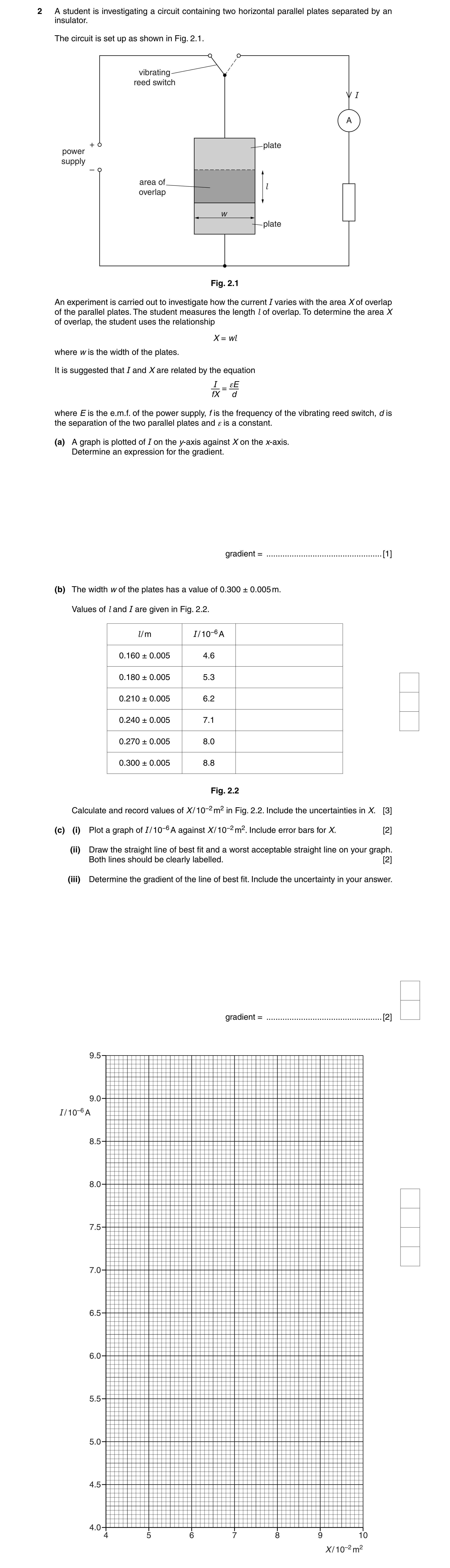
2 A student is investigating a circuit containing two horizontal parallel plates separated by an insulator. The circuit is set up as shown in Fig. 2.1. vibrating reed switch I A + plate power supply – area of l overlap w plate Fig. 2.1 An experiment is carried out to investigate how the current I varies with the area X of overlap of the parallel plates. The student measures the length l of overlap. To determine the area X of overlap, the student uses the relationship X = wl where w is the width of the plates. It is suggested that I and X are related by the equation I εE = fX d where E is the e.m.f. of the power supply, f is the frequency of the vibrating reed switch, d is the separation of the two parallel plates and ε is a constant. (a) A graph is plotted of I on the y-axis against X on the x-axis. Determine an expression for the gradient. gradient = … [1] (b) The width w of the plates has a value of 0.300 ± 0.005 m. Values of l and I are given in Fig. 2.2. l / m I / 10−6 A 0.160 ± 0.005 4.6 0.180 ± 0.005 5.3 0.210 ± 0.005 6.2 0.240 ± 0.005 7.1 0.270 ± 0.005 8.0 0.300 ± 0.005 8.8 Fig. 2.2 Calculate and record values of X / 10−2 m2 in Fig. 2.2. Include the uncertainties in X. [3] (c) (i) Plot a graph of I / 10−6 A against X / 10−2 m2. Include error bars for X. [2] (ii) Draw the straight line of best fit and a worst acceptable straight line on your graph. Both lines should be clearly labelled. [2] (iii) Determine the gradient of the line of best fit. Include the uncertainty in your answer. gradient = … [2] 9.5 9.0 I / 10–6 A 8.5 8.0 7.5 7.0 6.5 6.0 5.5 5.0 4.5 4.0 4 5 6 7 8 9 10 X / 10–2 m2
10 marks
Mark scheme: 2 Analysis, conclusions and evaluation (15 marks) Expected Answer Additional Guidance ε Ef (a) A1 gradient = d (b) T1 X / 10–2 m2 T2 Allow a mixture of significant figures. 4.80 or 4.800 Must be table values. 5.40 or 5.400 6.30 or 6.300 7.20 or 7.200 8.10 or 8.100 9.00 or 9.000 U1 From ±0.2 to ±0.3 Allow more than one significant figure. (c) (i) G1 Six points plotted correctly Must be within half a small square. Do not allow “blobs”. Ecf allowed from table. U2 Error bars in X plotted All error bars to be plotted. Must be accurate to correctly less than half a small square. (ii) G2 Line of best fit Lower end of line must pass between (5.1, 5.0) and (5.3, 5.0) and upper end of line must pass between (8.5, 8.5) and (8.8, 8.5). G3 Worst acceptable straight line. Line should be clearly labelled or dashed. Steepest or shallowest Examiner judgement on worst acceptable line. possible line that passes Lines must cross. Mark scored only if error bars through all the error bars. are plotted. (iii) C1 Gradient of best fit line The triangle used should be at least half the length of the drawn line. Check the read-offs. Work to half a small square. Do not penalise POT. (Should be about 1 × 10⁻⁴.) U3 Uncertainty in gradient Method of determining absolute uncertainty: difference in worst gradient and gradient. (d) (i) C2 ε = 6.25 × 10⁻⁷ × gradient Do not penalise POT. (Should be about 6 or 7 × 10–11.) C3 F m–1 or C V–1 m–1 Allow A m–1 V–1 Hz–1 or A s m–1 V–1 or A2 s4 kg–1 m–3. Power of 10 must be correct. (ii) U4 Percentage uncertainty in ε 10.83% + percentage uncertainty in gradient (e) C4 f in the range 73.0 to 84.4 and Allow 73 to 84 for 2 s.f. given to 2 or 3 s.f. 5 . 0 × 10 −9 f = ε U5 Absolute uncertainty in f Clear working needed. Allow ecf from (d)(ii). Uncertainties in Question 2 (c) (iii) Gradient [U3] uncertainty = gradient of line of best fit – gradient of worst acceptable line uncertainty = ½ (steepest worst line gradient – shallowest worst line gradient) (d) (ii) [U4] max gradient × max d max ε = min E × min f min gradient × min d min ε = max E × max f ∆gradient ∆d ∆f ∆E + + + × 100 % uncertainty = d f E gradient ∆gradient 0.0002 10 0.2 = + + + × 100 gradient 0.0030 400 12.0 (e) [U5] max I × max d max f = min X × min ε × min E min I × min d min f = max X × max ε × max E ∆I ∆d ∆l ∆E ∆ε 0.1 0.0002 0.001 0.2 ∆ε ∆ε ∆f = + + 2 + + f = + + 2 + + f = 0.107 + f I d l E ε 5.0 0.0030 0.500 12.0 ε ε 10.7 + (d)(ii) 21.5 + % uncertainty in gradient ∆f = f = f if (d)(ii) is correct 100 100
This question in 9702/52 May/June 2015
Q7 · A student is investigating a circuit containing capacitors 9702/53 Oct/Nov 2016
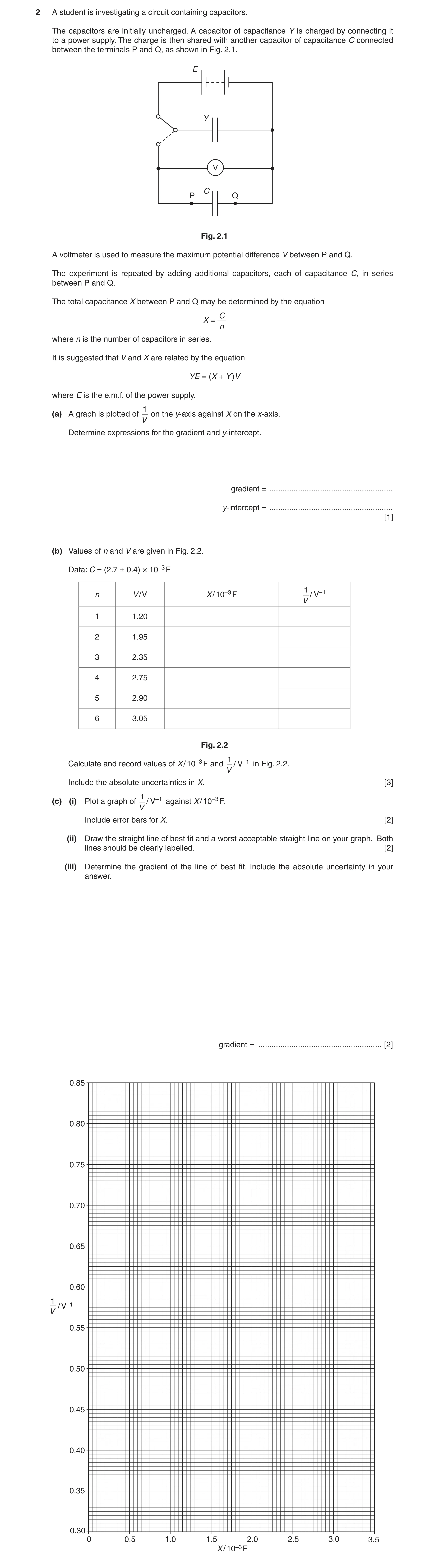
2 A student is investigating a circuit containing capacitors. The capacitors are initially uncharged. A capacitor of capacitance Y is charged by connecting it to a power supply. The charge is then shared with another capacitor of capacitance C connected between the terminals P and Q, as shown in Fig. 2.1. E Y V C P Q Fig. 2.1 A voltmeter is used to measure the maximum potential difference V between P and Q. The experiment is repeated by adding additional capacitors, each of capacitance C, in series between P and Q. The total capacitance X between P and Q may be determined by the equation C X = n where n is the number of capacitors in series. It is suggested that V and X are related by the equation YE = (X + Y )V where E is the e.m.f. of the power supply. 1 (a) A graph is plotted of on the y-axis against X on the x-axis. V Determine expressions for the gradient and y-intercept. gradient = … y-intercept = … [1] (b) Values of n and V are given in Fig. 2.2. Data: C = (2.7 ± 0.4) × 10–3 F 1 n V / V X / 10–3 F / V–1 V 1 1.20 2 1.95 3 2.35 4 2.75 5 2.90 6 3.05 Fig. 2.2 1 Calculate and record values of X / 10–3 F and / V–1 in Fig. 2.2. V Include the absolute uncertainties in X. [3] 1(c) (i) Plot a graph of / V–1 against X / 10–3 F. V Include error bars for X. [2] (ii) Draw the straight line of best fit and a worst acceptable straight line on your graph. Both lines should be clearly labelled. [2] (iii) Determine the gradient of the line of best fit. Include the absolute uncertainty in your answer. gradient = … [2] 0.85 0.80 0.75 0.70 0.65 0.60 1 / V–1V 0.55 0.50 0.45 0.40 0.35 0.30 0 0.5 1.0 1.5 2.0 2.5 3.0 3.5 X / 10–3 F
10 marks
Mark scheme: 2 (a) 1 1 gradient = YE 1 y-intercept = E (b) 2.7 or 2.70 0.833 or 0.8333 1.4 or 1.35 0.513 or 0.5128 0.90 or 0.900 0.426 or 0.4255 0.68 or 0.675 0.364 or 0.3636 0.54 or 0.540 0.345 or 0.3448 0.45 or 0.450 0.328 or 0.3279 All first column correct. Allow a mixture of significant figures. 1 All second column correct. Allow a mixture of significant figures. 1 Uncertainties in X from ± 0.4 to ± 0.07 (± 0.1). Allow more than one significant figure. 1 (c) (i) Six points plotted correctly. 1 Must be within half a small square. No “blobs”. All error bars in X plotted correctly. 1 All error bars to be plotted. Length of bar must be accurate to less than half a small square and symmetrical. (ii) Line of best fit drawn. 1 Line must not be drawn from top point to bottom point. The lower end of line should pass between (0.95, 0.45) and (1.1, 0.45) and upper end of line should pass between (2.10, 0.70) and (2.25, 0.70). Worst acceptable line drawn correctly. 1 Steepest or shallowest possible line that passes through all the error bars. Mark scored only if all error bars are plotted. (iii) Gradient determined with a triangle that is at least half the length of the 1 drawn line. Read-offs must be accurate to half a small square. Method of determining absolute uncertainty. 1 uncertainty = gradient of line of best fit – gradient of worst acceptable line or uncertainty = ½(steepest worst line gradient – shallowest worst line gradient) (iv) y-intercept determined correctly by substitution into y = mx + c. 1 Read-offs must be accurate to half a small square. Method of determining absolute uncertainty. 1 uncertainty = y-intercept of line of best fit – y-intercept of worst acceptable line or uncertainty = ½(steepest worst line y-intercept – shallowest worst line y-intercept) No ECF from false origin method. (d) (i) E = 1/y-intercept and given to 2 or 3 s.f. 1 1 1 y − intercept Y = or E × gradient gradient Y in the range (0.90 to 1.20) × 10–3 F. Appropriate unit required. Correct substitution of numbers must be seen. (ii) Percentage uncertainty in Y 1 ∆m ∆c = + × 100 or m c ∆m ∆ E = + × 100 or m E ∆Y = × 100 Y Maximum/minimum methods: 1 max y − intercept max Y = = min E × min gradient min gradient 1 min y − intercept min Y = = max E × max gradient max gradient
This question in 9702/53 Oct/Nov 2016
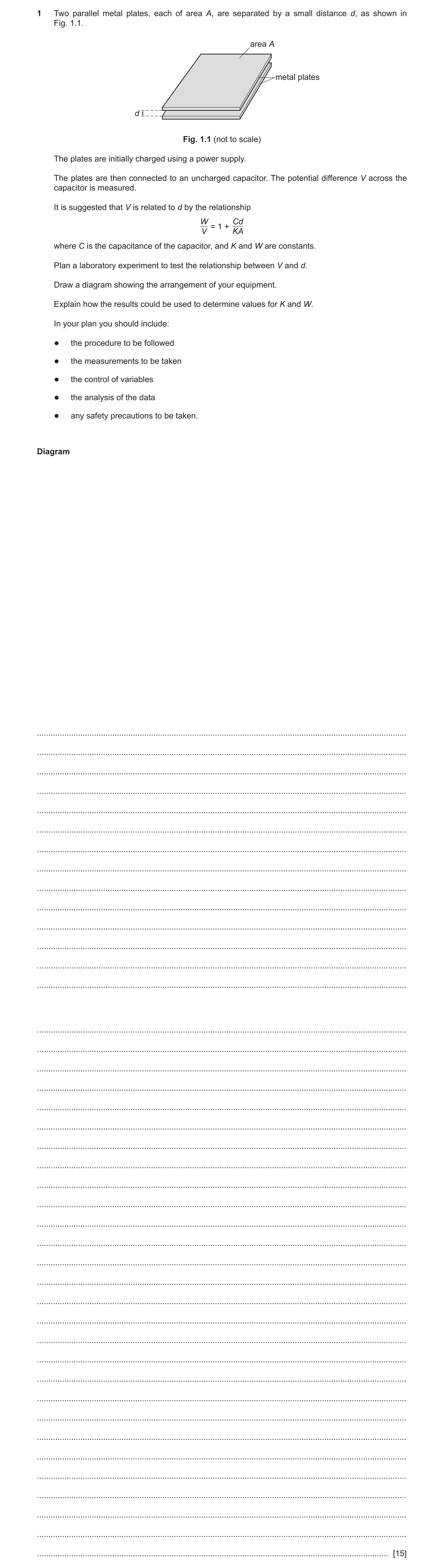
Q8 · Two parallel metal plates, each of area A, are separated by a small distance d, as shown… 9702/51 May/June 2022
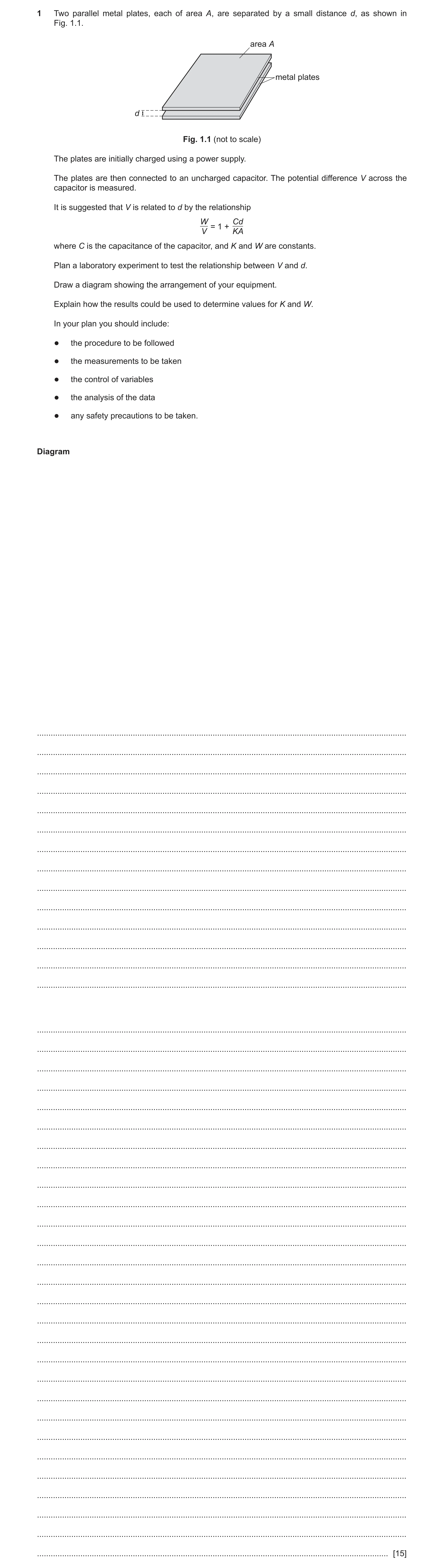
1 Two parallel metal plates, each of area A, are separated by a small distance d, as shown in Fig. 1.1. area A metal plates d Fig. 1.1 (not to scale) The plates are initially charged using a power supply. The plates are then connected to an uncharged capacitor. The potential difference V across the capacitor is measured. It is suggested that V is related to d by the relationship W Cd = 1 + V KA where C is the capacitance of the capacitor, and K and W are constants. Plan a laboratory experiment to test the relationship between V and d. Draw a diagram showing the arrangement of your equipment. Explain how the results could be used to determine values for K and W. In your plan you should include: ● the procedure to be followed ● the measurements to be taken ● the control of variables ● the analysis of the data ● any safety precautions to be taken. Diagram … … … … … … … … … … … … … … … … … … … … … … … … … … … … … … … … … … … … … … … … … … [15]
15 marks
Mark scheme: 1 Defining the problem d is the independent variable and V is the dependent variable or vary d and measure V 1 keep A or area (of overlap) of plates constant 1 Methods of data collection labelled diagram of workable experiment including: circuit diagram with voltmeter connected in parallel with the capacitor capacitor and voltmeter connected to the metal plates with no power supply in discharge part of the circuit correct symbols for capacitor and voltmeter 1 method to charge parallel plates, e.g. separate circuit diagram showing plates connected to a d.c. power supply or combined circuit with switches and d.c. power supply 1 use calipers to measure d or use micrometer/calipers to measure thickness of spacers 1 use rule(r) to measure lengths to determine A and A = length breadth 1 Method of analysis plot a graph of 1 V against d or equivalent (e.g. d against 1 V ) (Do not accept log graphs.) 1 -intercept or gradient gradient y C C K K A AW (for d against 1 V : -intercept y C K A ) 1 Question Answer Marks 1 1 -intercept W y (for d against 1 V : gradient or -intercept W y gradient C W AK ) 1 Additional detail including safety considerations 6 D1 use gloves to prevent electric shock or do not touch metal plates to avoid shocks D2 keep the initial p.d. across plates or initial charge constant D3 method to determine the value of C, e.g. description of an experiment to measure p.d. or current against time during discharge through a resistor D4 method of operation of circuit(s) using switch(es) D5 description of method to fully discharge capacitor, e.g. between experiments, short-circuit the capacitor or use of switch in parallel with capacitor D6 repeat measurements of d at different points across plates and average D7 repeat measurements of V for same d and average V D8 bottom plate resting on insulating material or top plate supported by strings D9 use high voltage power supply to increase charge on plates or use a very small value of capacitance to increase voltmeter reading D10 relationship valid if a straight line is produced (not passing through the origin)
This question in 9702/51 May/June 2022
Q9 · Two parallel metal plates, each of area A, are separated by a small distance d, as shown… 9702/53 May/June 2022
1 Two parallel metal plates, each of area A, are separated by a small distance d, as shown in Fig. 1.1. area A metal plates d Fig. 1.1 (not to scale) The plates are initially charged using a power supply. The plates are then connected to an uncharged capacitor. The potential difference V across the capacitor is measured. It is suggested that V is related to d by the relationship W Cd = 1 + V KA where C is the capacitance of the capacitor, and K and W are constants. Plan a laboratory experiment to test the relationship between V and d. Draw a diagram showing the arrangement of your equipment. Explain how the results could be used to determine values for K and W. In your plan you should include: ● the procedure to be followed ● the measurements to be taken ● the control of variables ● the analysis of the data ● any safety precautions to be taken. Diagram … … … … … … … … … … … … … … … … … … … … … … … … … … … … … … … … … … … … … … … … … … [15]
15 marks
Mark scheme: 1 Defining the problem d is the independent variable and V is the dependent variable or vary d and measure V 1 keep A or area (of overlap) of plates constant 1 Methods of data collection labelled diagram of workable experiment including: circuit diagram with voltmeter connected in parallel with the capacitor capacitor and voltmeter connected to the metal plates with no power supply in discharge part of the circuit correct symbols for capacitor and voltmeter 1 method to charge parallel plates, e.g. separate circuit diagram showing plates connected to a d.c. power supply or combined circuit with switches and d.c. power supply 1 use calipers to measure d or use micrometer/calipers to measure thickness of spacers 1 use rule(r) to measure lengths to determine A and A = length breadth 1 Method of analysis plot a graph of 1 V against d or equivalent (e.g. d against 1 V ) (Do not accept log graphs.) 1 -intercept or gradient gradient y C C K K A AW (for d against 1 V : -intercept y C K A ) 1 Question Answer Marks 1 1 -intercept W y (for d against 1 V : gradient or -intercept W y gradient C W AK ) 1 Additional detail including safety considerations 6 D1 use gloves to prevent electric shock or do not touch metal plates to avoid shocks D2 keep the initial p.d. across plates or initial charge constant D3 method to determine the value of C, e.g. description of an experiment to measure p.d. or current against time during discharge through a resistor D4 method of operation of circuit(s) using switch(es) D5 description of method to fully discharge capacitor, e.g. between experiments, short-circuit the capacitor or use of switch in parallel with capacitor D6 repeat measurements of d at different points across plates and average D7 repeat measurements of V for same d and average V D8 bottom plate resting on insulating material or top plate supported by strings D9 use high voltage power supply to increase charge on plates or use a very small value of capacitance to increase voltmeter reading D10 relationship valid if a straight line is produced (not passing through the origin)
This question in 9702/53 May/June 2022
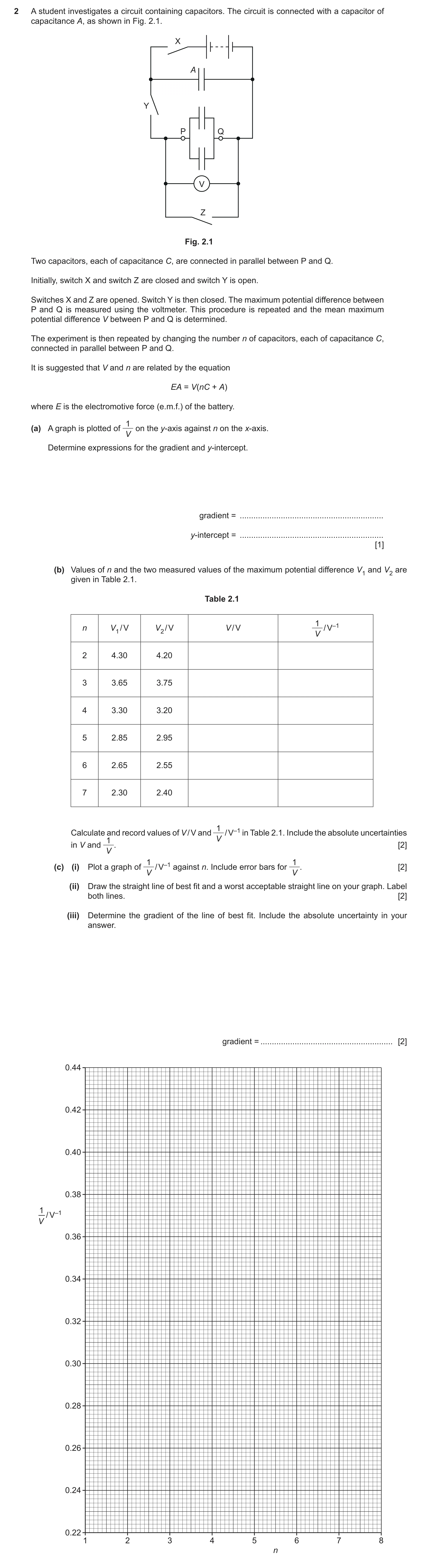
Q10 · A student investigates a circuit containing capacitors 9702/52 May/June 2025
2 A student investigates a circuit containing capacitors. The circuit is connected with a capacitor of capacitance A, as shown in Fig. 2.1. X A Y P Q V Z Fig. 2.1 Two capacitors, each of capacitance C, are connected in parallel between P and Q. Initially, switch X and switch Z are closed and switch Y is open. Switches X and Z are opened. Switch Y is then closed. The maximum potential difference between P and Q is measured using the voltmeter. This procedure is repeated and the mean maximum potential difference V between P and Q is determined. The experiment is then repeated by changing the number n of capacitors, each of capacitance C, connected in parallel between P and Q. It is suggested that V and n are related by the equation EA = V(nC + A) where E is the electromotive force (e.m.f.) of the battery. 1 (a) A graph is plotted of on the y-axis against n on the x-axis. V Determine expressions for the gradient and y-intercept. gradient = … y-intercept = … [1] (b) Values of n and the two measured values of the maximum potential difference V1 and V2 are given in Table 2.1. Table 2.1 1 n V1 / V V2 / V V / V / V–1 V 2 4.30 4.20 3 3.65 3.75 4 3.30 3.20 5 2.85 2.95 6 2.65 2.55 7 2.30 2.40 1 Calculate and record values of V / V and / V–1 in Table 2.1. Include the absolute uncertainties 1 V in V and . [2] V 1 1(c) (i) Plot a graph of / V–1 against n. Include error bars for . [2] V V (ii) Draw the straight line of best fit and a worst acceptable straight line on your graph. Label both lines. [2] (iii) Determine the gradient of the line of best fit. Include the absolute uncertainty in your answer. gradient = … [2]
9 marks
Mark scheme: 2(a) C 1 gradient = EA 1 y-intercept = E 2(b) 1 1 V / V / V–1 V 4.25 0.235 or 0.2353 3.70 0.270 or 0.2703 3.25 0.308 or 0.3077 2.90 0.345 or 0.3448 2.60 0.385 or 0.3846 2.35 0.426 or 0.4255 1 Values of V / V and / V–1 correct as shown above. V Uncertainties in V all 0.05 1 and 1 uncertainties in from 0.002 or 0.003 increasing to 0.009. V 2(c)(i) Six points from (b) plotted correctly. 1 Must be within half a small square. Diameter of points must be less than half a small square. 1 1 Error bars in plotted correctly. V All error bars must be plotted. Total length of bar must be accurate to less than half a small square and symmetrical. 2(c)(ii) Straight line of best fit drawn. 1 Thickness of the line must be less than half a small square. Do not accept line from top point to bottom point. Line must pass between (2.65, 0.26) and (2.80, 0.26) and between (6.30, 0.40) and (6.50, 0.40). Worst acceptable straight line drawn (steepest or shallowest possible line that passes through all the error bars). 1 Thickness of the line must be less than half a small square. All error bars must be plotted. 2(c)(iii) Gradient determined with clear substitution of data points into y / x. 1 Distance between data points must be greater than half the length of the drawn line. Gradient determined of worst acceptable line with clear substitution of data points into y / x. 1 uncertainty = (gradient of line of best fit – gradient of worst acceptable line) or uncertainty = ½ (steepest worst line gradient – shallowest worst line gradient) 2(c)(iv) y-intercept determined by substitution of correct point into y = mx + c. 1 y-intercept of worst acceptable line determined by substitution into y = mx + c. 1 uncertainty = y-intercept of line of best fit – y-intercept of worst acceptable line or uncertainty = ½ (steepest worst line y-intercept – shallowest worst line y-intercept) Do not accept ECF from false origin method. 2(d)(i) E determined using y-intercept and E and C given to 2 or 3 significant figures. 1 1 E = y -intercept C determined using gradient and E and C given with correct units with appropriate powers of ten. 1 A gradient C = or C = A E gradient y -intercept unit of E: V unit of C: F 2(d)(ii) Percentage uncertainty determined with method shown. 1 A gradient y -intercept C % = + + 100 A gradient y -intercept or A gradient E C % = + + 100 with method to determine E shown A gradient E 2(e) V determined to a minimum of 2 significant figures from (c)(iii) and (c)(iv) or (d)(i) with correct substitution. 1 1 V = 10 gradient+y -intercept or EA V = 10C + A
This question in 9702/52 May/June 2025
 10
10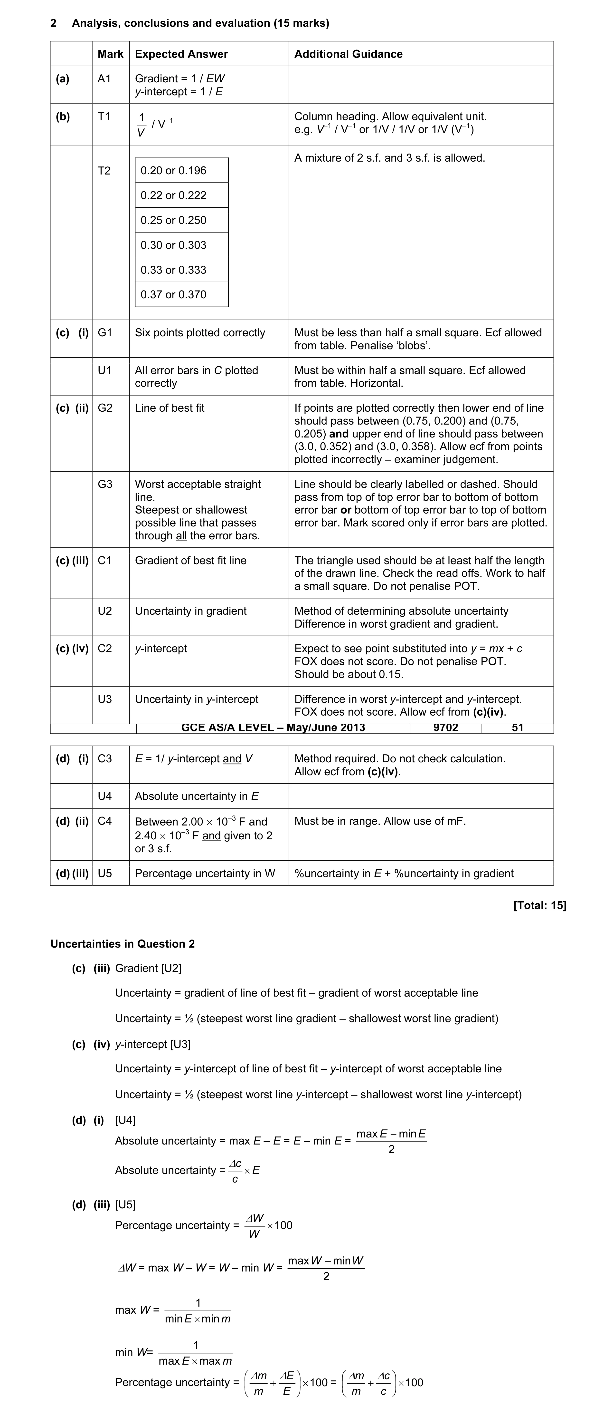 9
9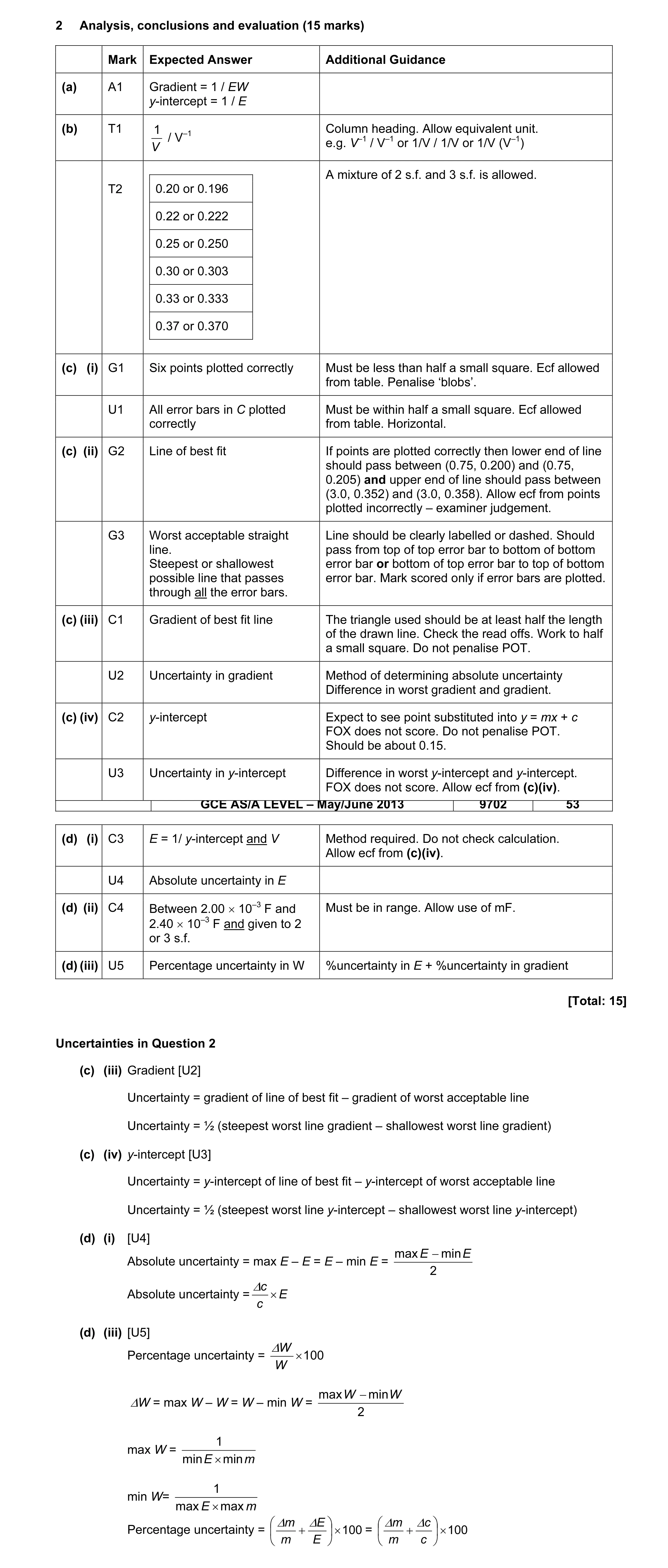 9
9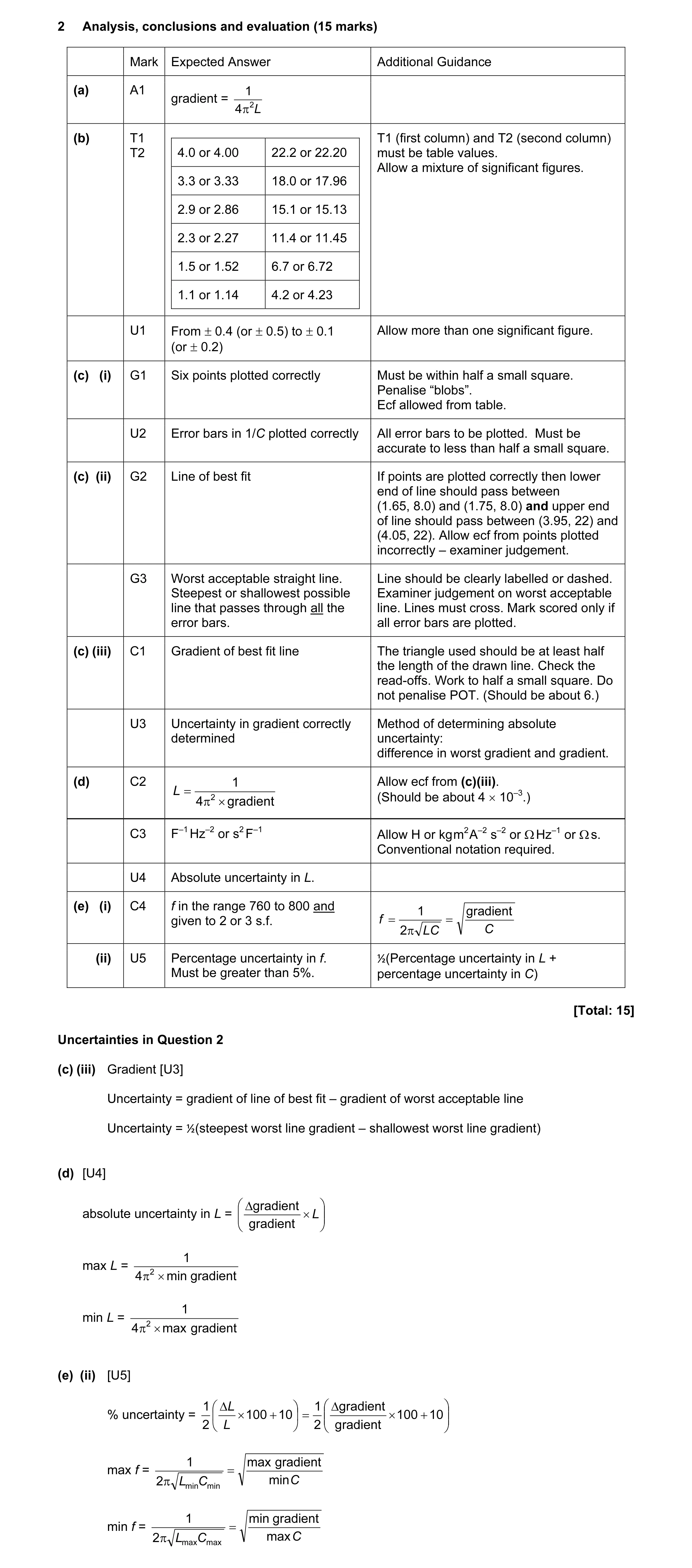 10
10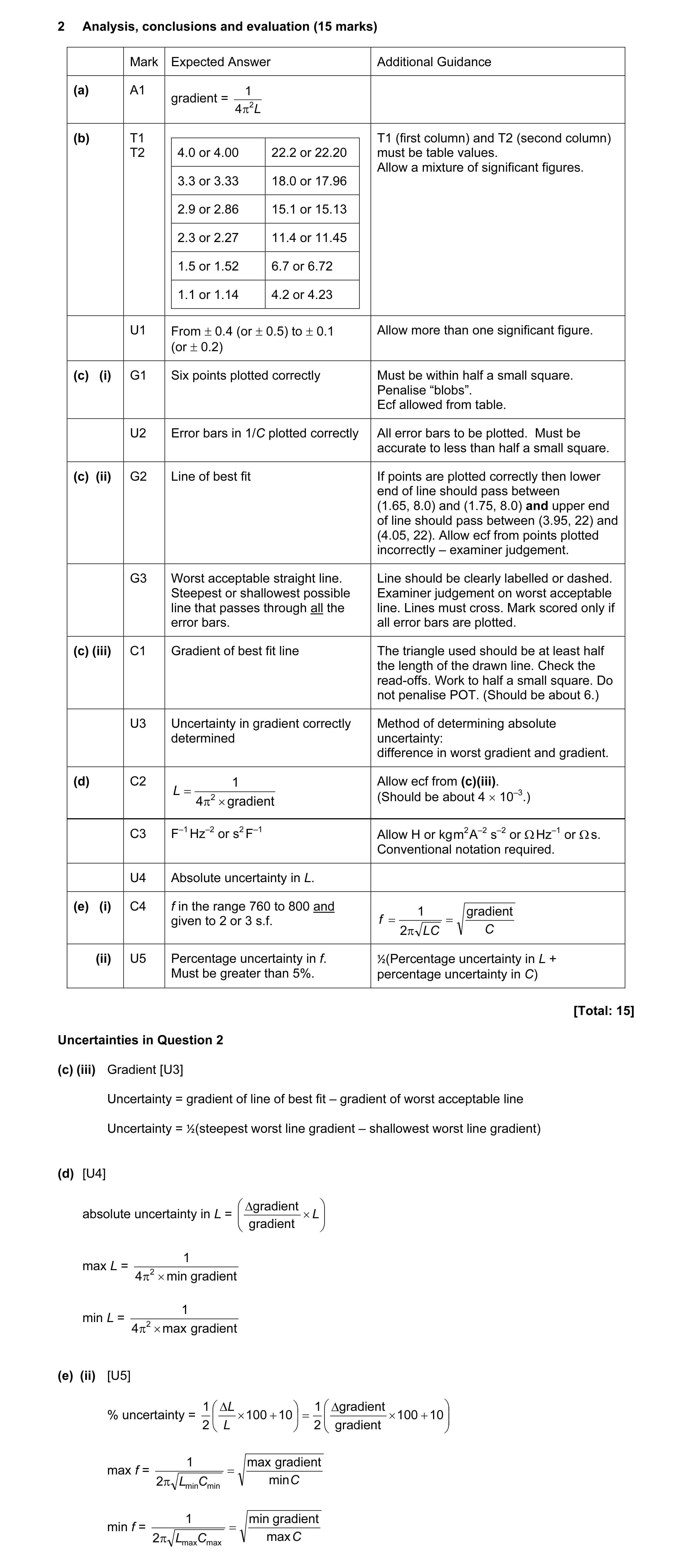 10
10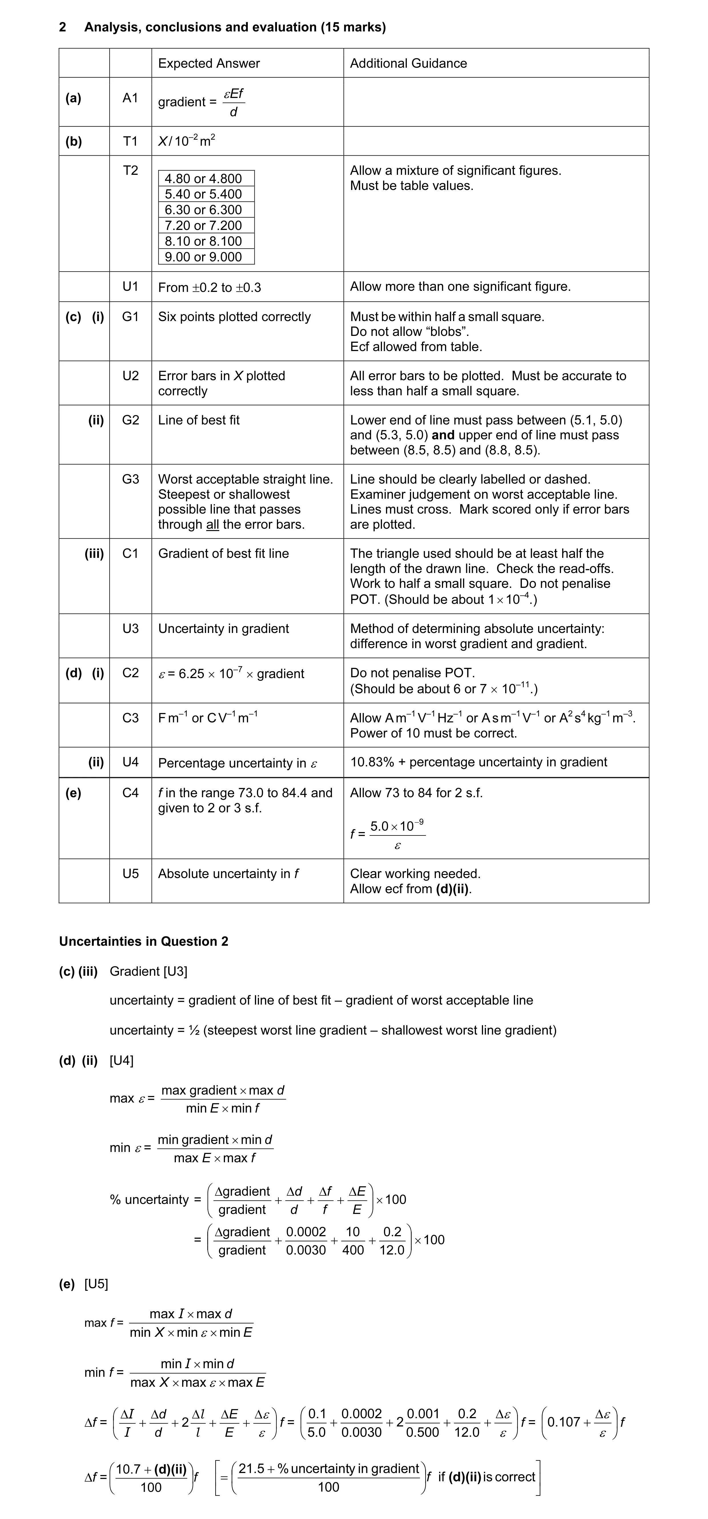 10
10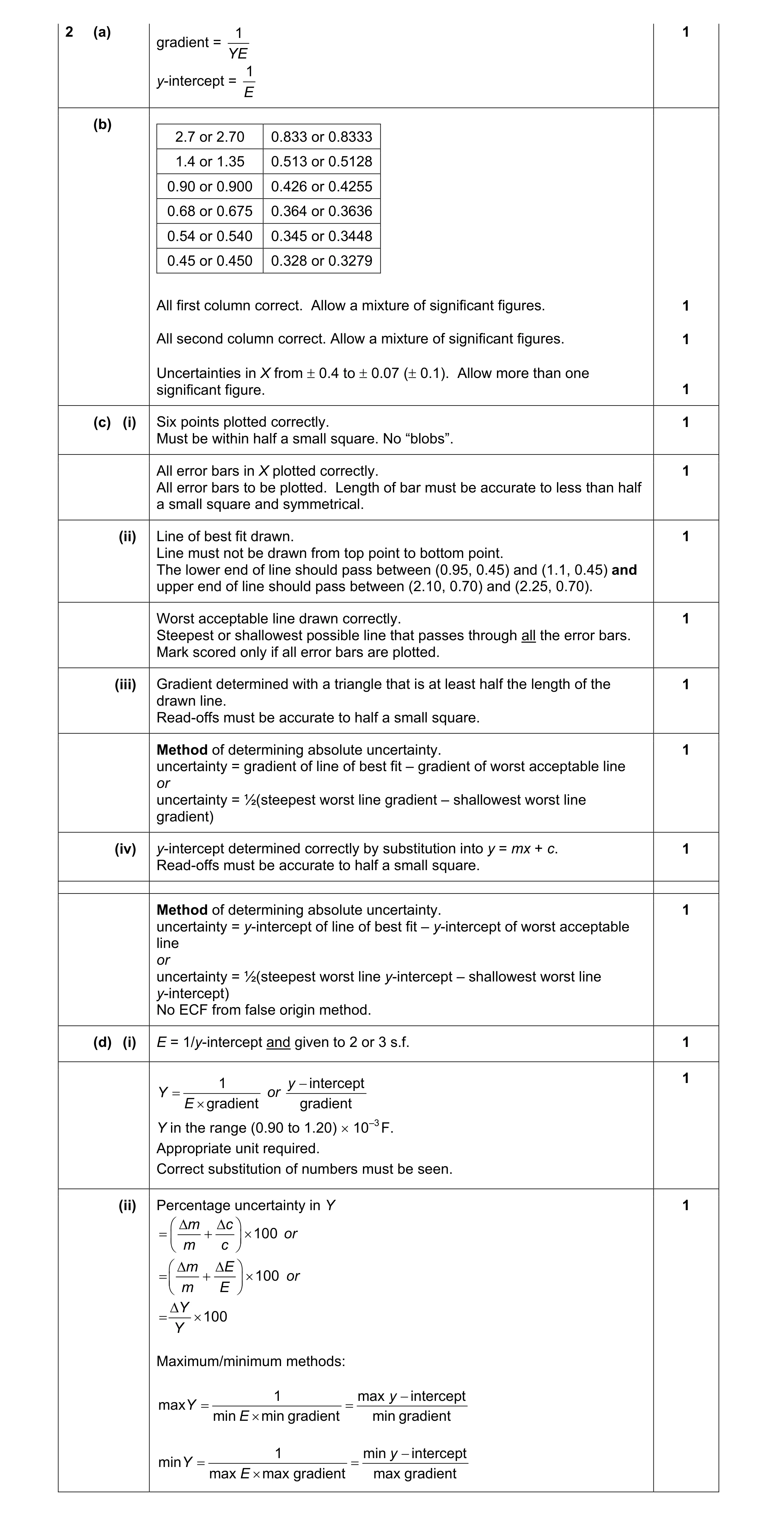 10
10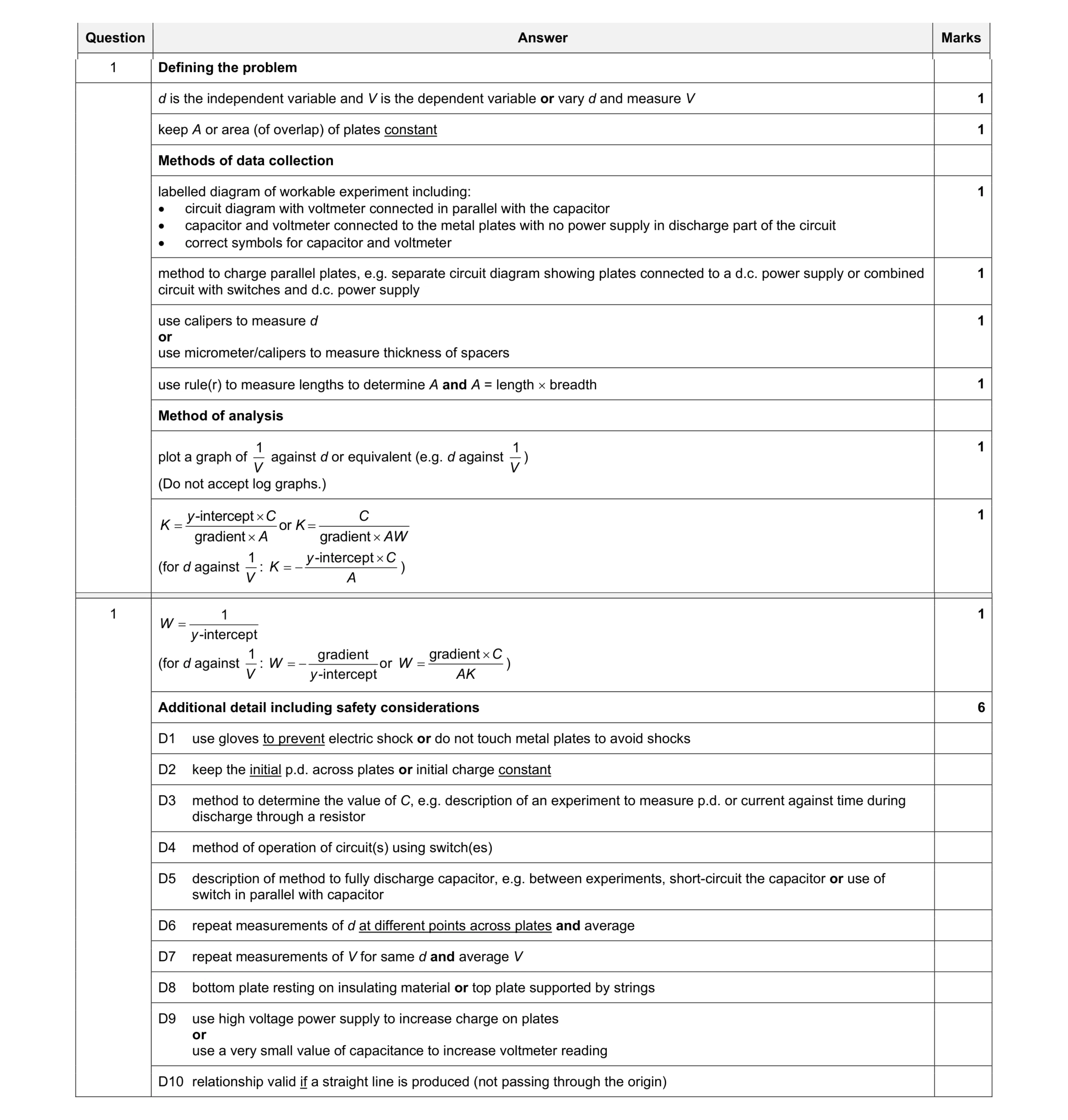 15
15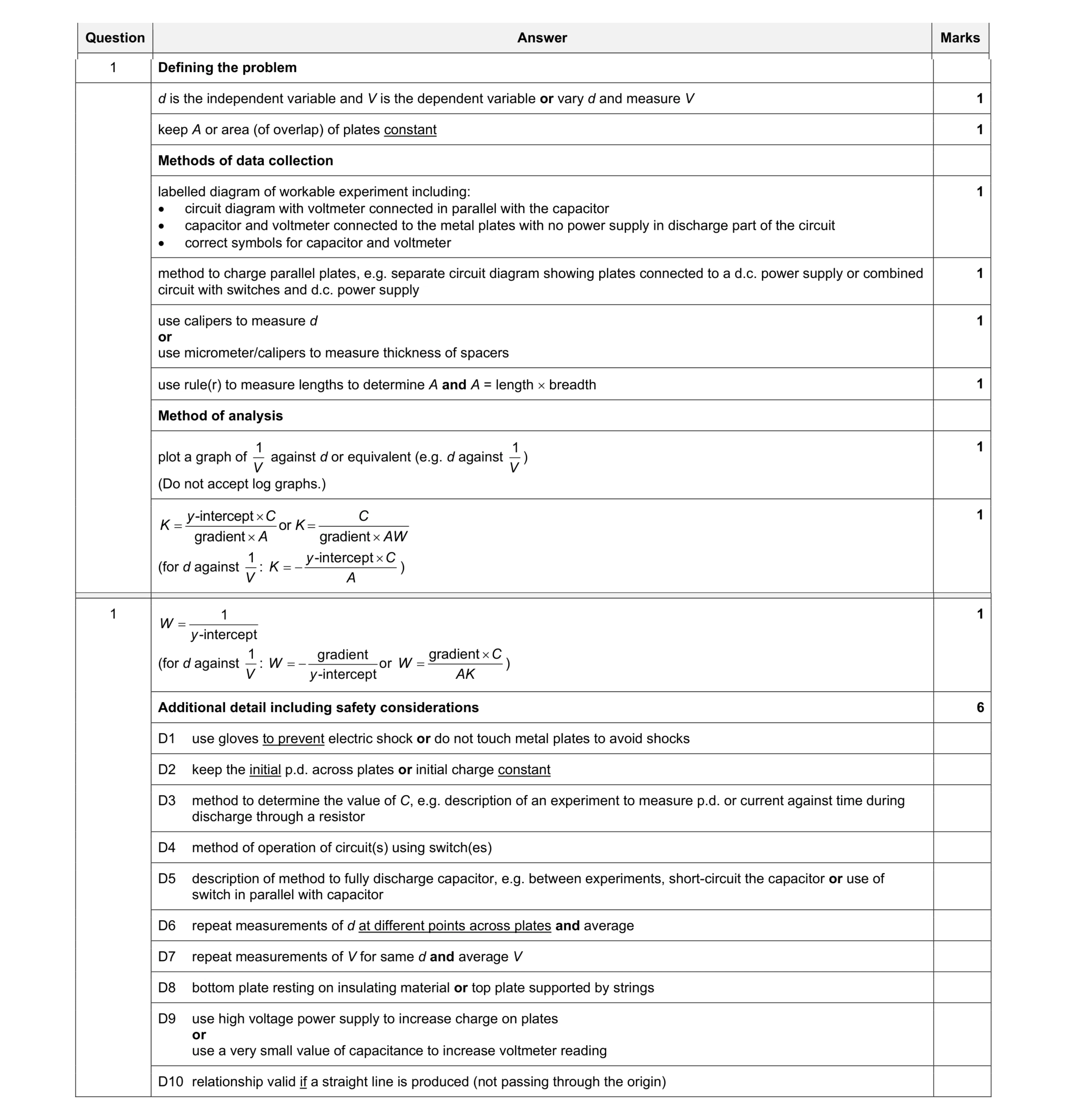 15
15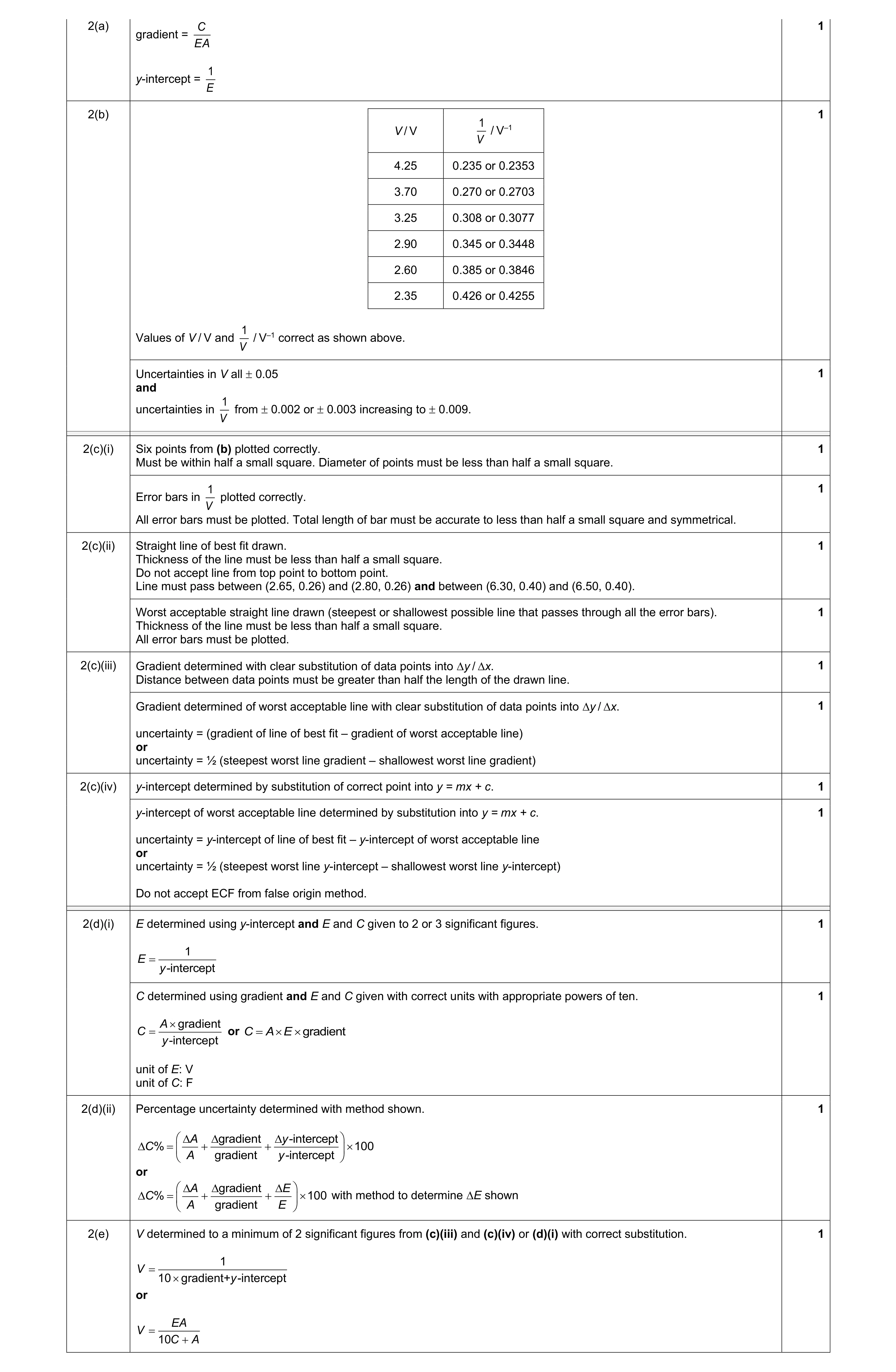 9
9