Cambridge A Level Applied Information and Communication Technology 9713 — 2012 May/June Paper 2 · Variant 1
9713/21/M/J/12 · 120 marks · ≈135 min
The question paper and its mark scheme, free to read here and free to download. This is Cambridge’s own paper, exactly as it was sat.
Question paper4 pages
Mark scheme13 pages
Answers below. Sit the paper first if you are practising.

Paper as text
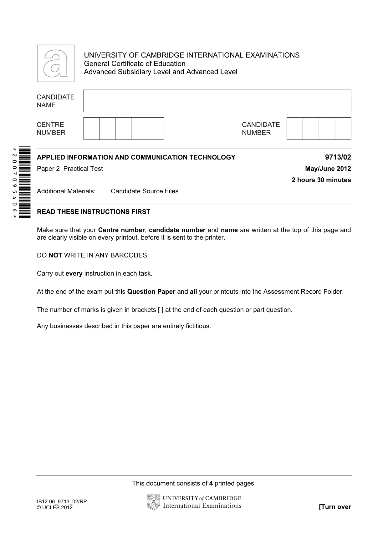
Question paper, page 1
This document consists of 4 printed pages. IB12 06_9713_02/RP © UCLES 2012 [Turn over *2007095406* UNIVERSITY OF CAMBRIDGE INTERNATIONAL EXAMINATIONS General Certificate of Education Advanced Subsidiary Level and Advanced Level APPLIED INFORMATION AND COMMUNICATION TECHNOLOGY 9713/02 Paper 2 Practical Test May/June 2012 2 hours 30 minutes Additional Materials: Candidate Source Files READ THESE INSTRUCTIONS FIRST Make sure that your Centre number, candidate number and name are written at the top of this page and are clearly visible on every printout, before it is sent to the printer. DO NOT WRITE IN ANY BARCODES. Carry out every instruction in each task. At the end of the exam put this Question Paper and all your printouts into the Assessment Record Folder. The number of marks is given in brackets [ ] at the end of each question or part question. Any businesses described in this paper are entirely fictitious.
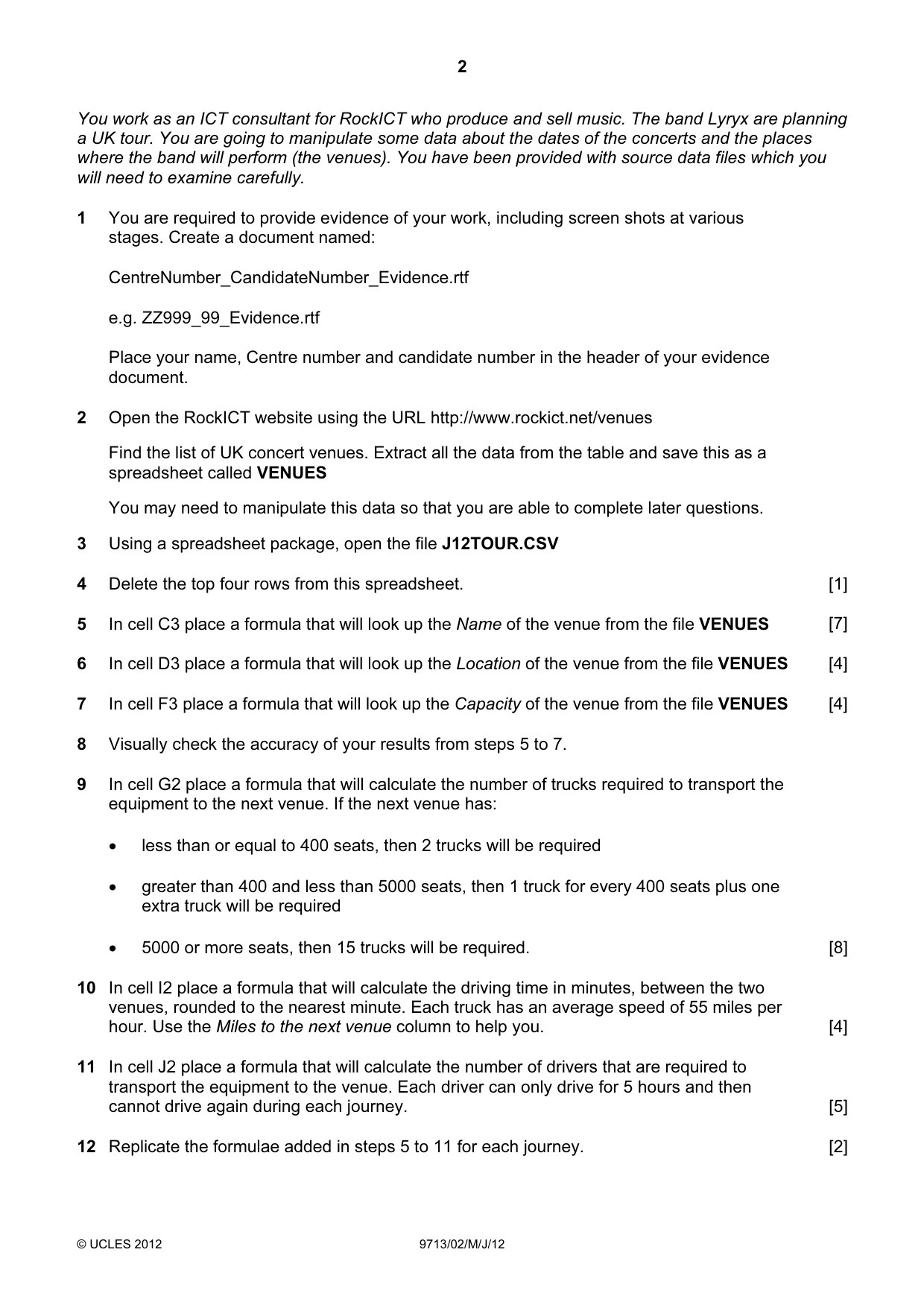
Question paper, page 2
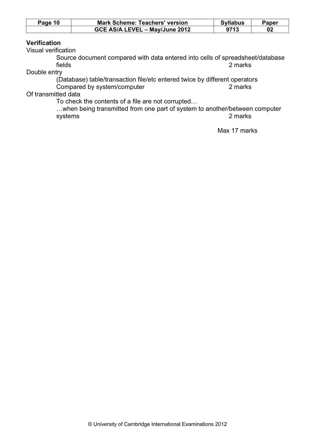
2 © UCLES 2012 9713/02/M/J/12 You work as an ICT consultant for RockICT who produce and sell music. The band Lyryx are planning a UK tour. You are going to manipulate some data about the dates of the concerts and the places where the band will perform (the venues). You have been provided with source data files which you will need to examine carefully. 1 You are required to provide evidence of your work, including screen shots at various stages. Create a document named: CentreNumber_CandidateNumber_Evidence.rtf e.g. ZZ999_99_Evidence.rtf Place your name, Centre number and candidate number in the header of your evidence document. 2 Open the RockICT website using the URL http://www.rockict.net/venues Find the list of UK concert venues. Extract all the data from the table and save this as a spreadsheet called VENUES You may need to manipulate this data so that you are able to complete later questions. 3 Using a spreadsheet package, open the file J12TOUR.CSV 4 Delete the top four rows from this spreadsheet. [1] 5 In cell C3 place a formula that will look up the Name of the venue from the file VENUES [7] 6 In cell D3 place a formula that will look up the Location of the venue from the file VENUES [4] 7 In cell F3 place a formula that will look up the Capacity of the venue from the file VENUES [4] 8 Visually check the accuracy of your results from steps 5 to 7. 9 In cell G2 place a formula that will calculate the number of trucks required to transport the equipment to the next venue. If the next venue has: • less than or equal to 400 seats, then 2 trucks will be required • greater than 400 and less than 5000 seats, then 1 truck for every 400 seats plus one extra truck will be required • 5000 or more seats, then 15 trucks will be required. [8] 10 In cell I2 place a formula that will calculate the driving time in minutes, between the two venues, rounded to the nearest minute. Each truck has an average speed of 55 miles per hour. Use the Miles to the next venue column to help you. [4] 11 In cell J2 place a formula that will calculate the number of drivers that are required to transport the equipment to the venue. Each driver can only drive for 5 hours and then cannot drive again during each journey. [5] 12 Replicate the formulae added in steps 5 to 11 for each journey. [2]
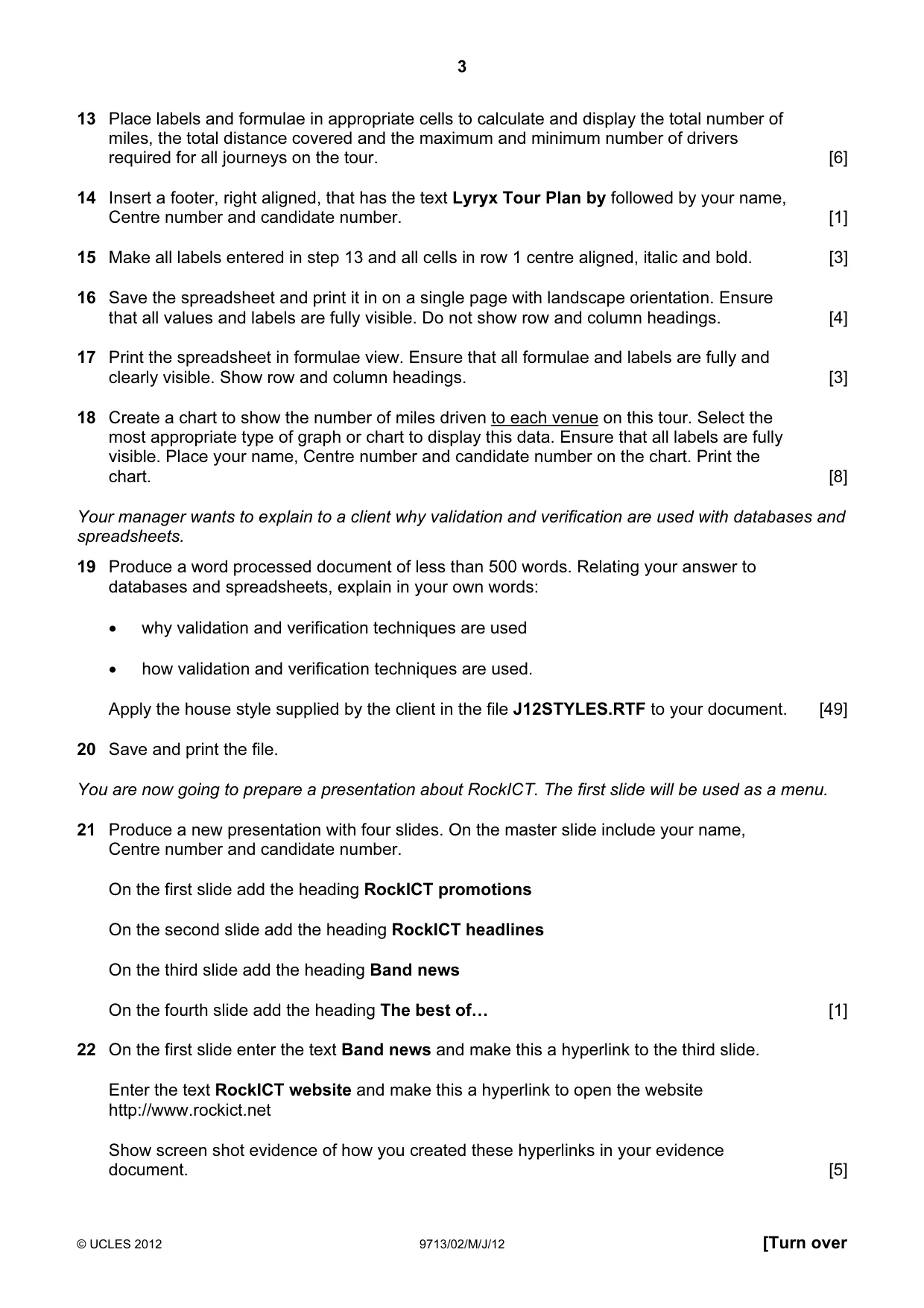
Question paper, page 3
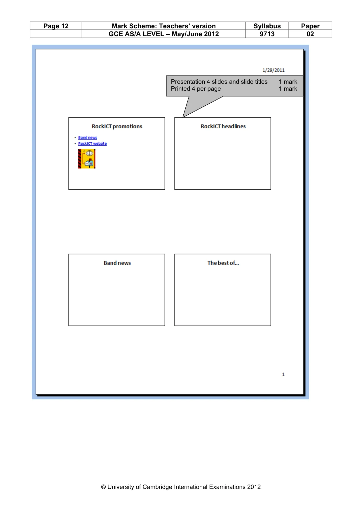
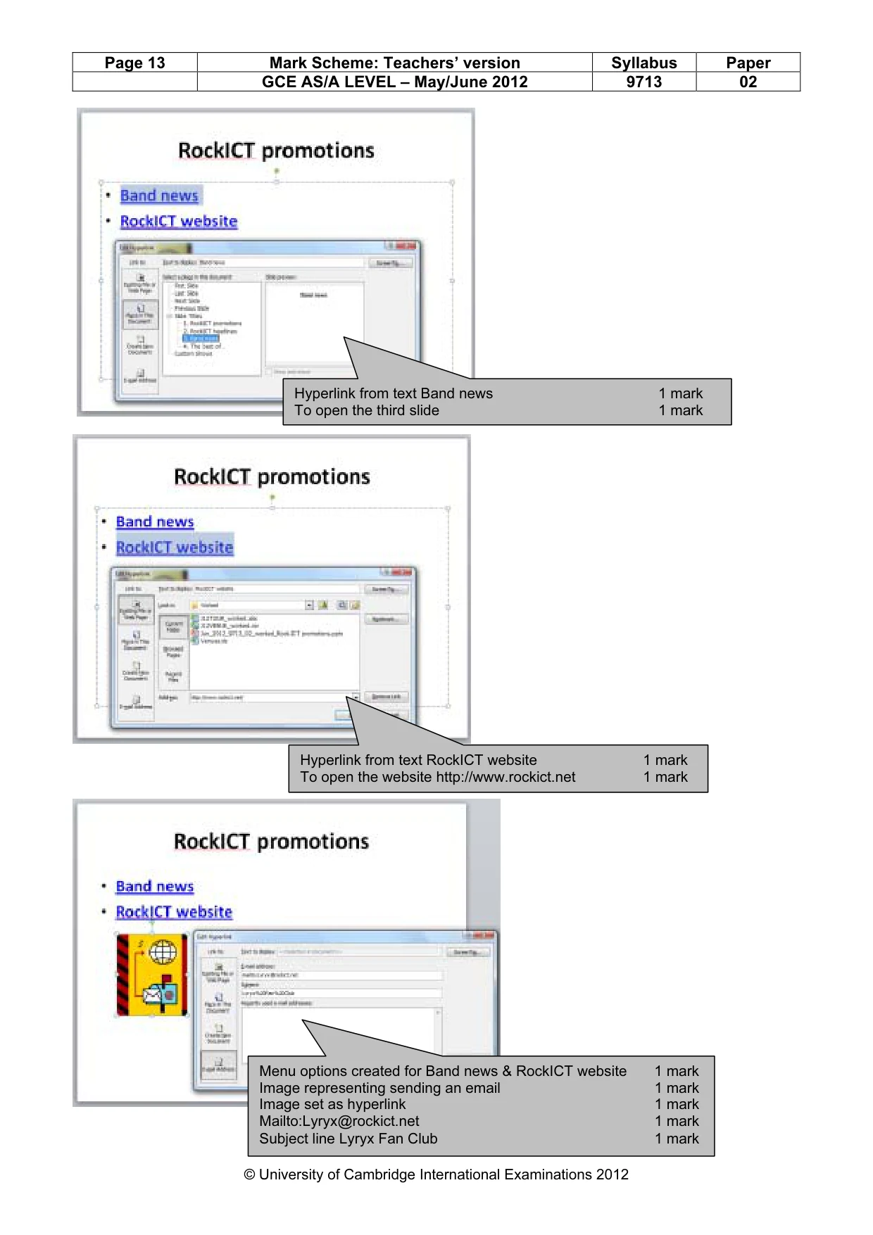
3 © UCLES 2012 9713/02/M/J/12 [Turn over 13 Place labels and formulae in appropriate cells to calculate and display the total number of miles, the total distance covered and the maximum and minimum number of drivers required for all journeys on the tour. [6] 14 Insert a footer, right aligned, that has the text Lyryx Tour Plan by followed by your name, Centre number and candidate number. [1] 15 Make all labels entered in step 13 and all cells in row 1 centre aligned, italic and bold. [3] 16 Save the spreadsheet and print it in on a single page with landscape orientation. Ensure that all values and labels are fully visible. Do not show row and column headings. [4] 17 Print the spreadsheet in formulae view. Ensure that all formulae and labels are fully and clearly visible. Show row and column headings. [3] 18 Create a chart to show the number of miles driven to each venue on this tour. Select the most appropriate type of graph or chart to display this data. Ensure that all labels are fully visible. Place your name, Centre number and candidate number on the chart. Print the chart. [8] Your manager wants to explain to a client why validation and verification are used with databases and spreadsheets. 19 Produce a word processed document of less than 500 words. Relating your answer to databases and spreadsheets, explain in your own words: • why validation and verification techniques are used • how validation and verification techniques are used. Apply the house style supplied by the client in the file J12STYLES.RTF to your document. [49] 20 Save and print the file. You are now going to prepare a presentation about RockICT. The first slide will be used as a menu. 21 Produce a new presentation with four slides. On the master slide include your name, Centre number and candidate number. On the first slide add the heading RockICT promotions On the second slide add the heading RockICT headlines On the third slide add the heading Band news On the fourth slide add the heading The best of… [1] 22 On the first slide enter the text Band news and make this a hyperlink to the third slide. Enter the text RockICT website and make this a hyperlink to open the website http://www.rockict.net Show screen shot evidence of how you created these hyperlinks in your evidence document. [5]
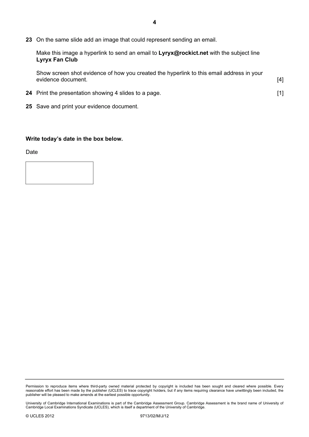
Question paper, page 4
4 Permission to reproduce items where third-party owned material protected by copyright is included has been sought and cleared where possible. Every reasonable effort has been made by the publisher (UCLES) to trace copyright holders, but if any items requiring clearance have unwittingly been included, the publisher will be pleased to make amends at the earliest possible opportunity. University of Cambridge International Examinations is part of the Cambridge Assessment Group. Cambridge Assessment is the brand name of University of Cambridge Local Examinations Syndicate (UCLES), which is itself a department of the University of Cambridge. © UCLES 2012 9713/02/M/J/12 23 On the same slide add an image that could represent sending an email. Make this image a hyperlink to send an email to Lyryx@rockict.net with the subject line Lyryx Fan Club Show screen shot evidence of how you created the hyperlink to this email address in your evidence document. [4] 24 Print the presentation showing 4 slides to a page. [1] 25 Save and print your evidence document. Write today’s date in the box below. Date
Mark scheme, page 1
UNIVERSITY OF CAMBRIDGE INTERNATIONAL EXAMINATIONS GCE Advanced Subsidiary Level and GCE Advanced Level MARK SCHEME for the May/June 2012 question paper for the guidance of teachers 9713 APPLIED ICT 9713/02 Paper 2 (Practical Test A), maximum raw mark 120 This mark scheme is published as an aid to teachers and candidates, to indicate the requirements of the examination. It shows the basis on which Examiners were instructed to award marks. It does not indicate the details of the discussions that took place at an Examiners’ meeting before marking began, which would have considered the acceptability of alternative answers. Mark schemes must be read in conjunction with the question papers and the report on the examination. • Cambridge will not enter into discussions or correspondence in connection with these mark schemes. Cambridge is publishing the mark schemes for the May/June 2012 question papers for most IGCSE, GCE Advanced Level and Advanced Subsidiary Level syllabuses and some Ordinary Level syllabuses.
Mark scheme, page 2
Page 2 Mark Scheme: Teachers’ version Syllabus Paper GCE AS/A LEVEL – May/June 2012 9713 02 © University of Cambridge International Examinations 2012 9713 – June 2012 AS Level – Paper 2 – Practical Test No marks to be awarded for any printout not containing the candidate name, candidate number and centre number
Mark scheme, page 3
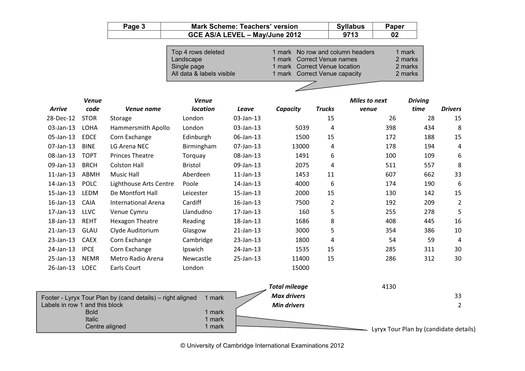
Page 3 Mark Scheme: Teachers’ version Syllabus Paper GCE AS/A LEVEL – May/June 2012 9713 02 © University of Cambridge International Examinations 2012 Arrive Venue code Venue name Venue location Leave Capacity Trucks Miles to next venue Driving time Drivers 28-Dec-12 STOR Storage London 03-Jan-13 15 26 28 15 03-Jan-13 LOHA Hammersmith Apollo London 03-Jan-13 5039 4 398 434 8 05-Jan-13 EDCE Corn Exchange Edinburgh 06-Jan-13 1500 15 172 188 15 07-Jan-13 BINE LG Arena NEC Birmingham 07-Jan-13 13000 4 178 194 4 08-Jan-13 TOPT Princes Theatre Torquay 08-Jan-13 1491 6 100 109 6 09-Jan-13 BRCH Colston Hall Bristol 09-Jan-13 2075 4 511 557 8 11-Jan-13 ABMH Music Hall Aberdeen 11-Jan-13 1453 11 607 662 33 14-Jan-13 POLC Lighthouse Arts Centre Poole 14-Jan-13 4000 6 174 190 6 15-Jan-13 LEDM De Montfort Hall Leicester 15-Jan-13 2000 15 130 142 15 16-Jan-13 CAIA International Arena Cardiff 16-Jan-13 7500 2 192 209 2 17-Jan-13 LLVC Venue Cymru Llandudno 17-Jan-13 160 5 255 278 5 18-Jan-13 REHT Hexagon Theatre Reading 18-Jan-13 1686 8 408 445 16 21-Jan-13 GLAU Clyde Auditorium Glasgow 21-Jan-13 3000 5 354 386 10 23-Jan-13 CAEX Corn Exchange Cambridge 23-Jan-13 1800 4 54 59 4 24-Jan-13 IPCE Corn Exchange Ipswich 24-Jan-13 1535 15 285 311 30 25-Jan-13 NEMR Metro Radio Arena Newcastle 25-Jan-13 11400 15 286 312 30 26-Jan-13 LOEC Earls Court London 15000 Total mileage 4130 Max drivers 33 Min drivers 2 Lyryx Tour Plan by (candidate details) Footer - Lyryx Tour Plan by (cand details) – right aligned 1 mark Labels in row 1 and this block Bold 1 mark Italic 1 mark Centre aligned 1 mark Footer - Lyryx Tour Plan by (cand details) – right aligned 1 mark Labels in row 1 and this block Bold 1 mark Italic 1 mark Centre aligned 1 mark Top 4 rows deleted 1 mark No row and column headers 1 mark Landscape 1 mark Correct Venue names 2 marks Single page 1 mark Correct Venue location 2 marks All data & labels visible 1 mark Correct Venue capacity 2 marks
Mark scheme, page 4
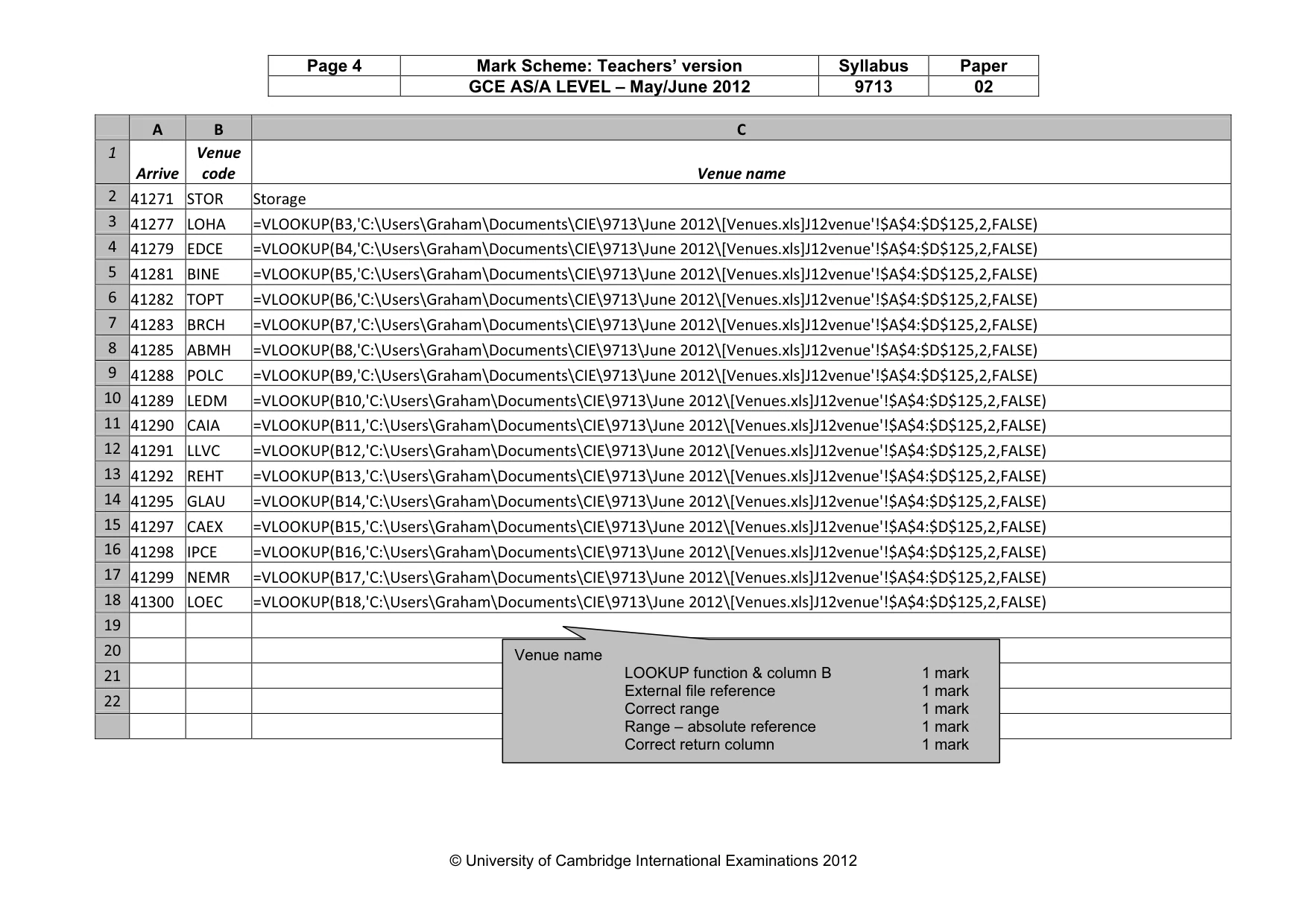
Page 4 Mark Scheme: Teachers’ version Syllabus Paper GCE AS/A LEVEL – May/June 2012 9713 02 © University of Cambridge International Examinations 2012 A B C 1 Arrive Venue code Venue name 2 41271 STOR Storage 3 41277 LOHA =VLOOKUP(B3,'C:\Users\Graham\Documents\CIE\9713\June 2012\[Venues.xls]J12venue'!$A$4:$D$125,2,FALSE) 4 41279 EDCE =VLOOKUP(B4,'C:\Users\Graham\Documents\CIE\9713\June 2012\[Venues.xls]J12venue'!$A$4:$D$125,2,FALSE) 5 41281 BINE =VLOOKUP(B5,'C:\Users\Graham\Documents\CIE\9713\June 2012\[Venues.xls]J12venue'!$A$4:$D$125,2,FALSE) 6 41282 TOPT =VLOOKUP(B6,'C:\Users\Graham\Documents\CIE\9713\June 2012\[Venues.xls]J12venue'!$A$4:$D$125,2,FALSE) 7 41283 BRCH =VLOOKUP(B7,'C:\Users\Graham\Documents\CIE\9713\June 2012\[Venues.xls]J12venue'!$A$4:$D$125,2,FALSE) 8 41285 ABMH =VLOOKUP(B8,'C:\Users\Graham\Documents\CIE\9713\June 2012\[Venues.xls]J12venue'!$A$4:$D$125,2,FALSE) 9 41288 POLC =VLOOKUP(B9,'C:\Users\Graham\Documents\CIE\9713\June 2012\[Venues.xls]J12venue'!$A$4:$D$125,2,FALSE) 10 41289 LEDM =VLOOKUP(B10,'C:\Users\Graham\Documents\CIE\9713\June 2012\[Venues.xls]J12venue'!$A$4:$D$125,2,FALSE) 11 41290 CAIA =VLOOKUP(B11,'C:\Users\Graham\Documents\CIE\9713\June 2012\[Venues.xls]J12venue'!$A$4:$D$125,2,FALSE) 12 41291 LLVC =VLOOKUP(B12,'C:\Users\Graham\Documents\CIE\9713\June 2012\[Venues.xls]J12venue'!$A$4:$D$125,2,FALSE) 13 41292 REHT =VLOOKUP(B13,'C:\Users\Graham\Documents\CIE\9713\June 2012\[Venues.xls]J12venue'!$A$4:$D$125,2,FALSE) 14 41295 GLAU =VLOOKUP(B14,'C:\Users\Graham\Documents\CIE\9713\June 2012\[Venues.xls]J12venue'!$A$4:$D$125,2,FALSE) 15 41297 CAEX =VLOOKUP(B15,'C:\Users\Graham\Documents\CIE\9713\June 2012\[Venues.xls]J12venue'!$A$4:$D$125,2,FALSE) 16 41298 IPCE =VLOOKUP(B16,'C:\Users\Graham\Documents\CIE\9713\June 2012\[Venues.xls]J12venue'!$A$4:$D$125,2,FALSE) 17 41299 NEMR =VLOOKUP(B17,'C:\Users\Graham\Documents\CIE\9713\June 2012\[Venues.xls]J12venue'!$A$4:$D$125,2,FALSE) 18 41300 LOEC =VLOOKUP(B18,'C:\Users\Graham\Documents\CIE\9713\June 2012\[Venues.xls]J12venue'!$A$4:$D$125,2,FALSE) 19 20 21 22 Venue name LOOKUP function & column B 1 mark External file reference 1 mark Correct range 1 mark Range – absolute reference 1 mark Correct return column 1 mark
Mark scheme, page 5
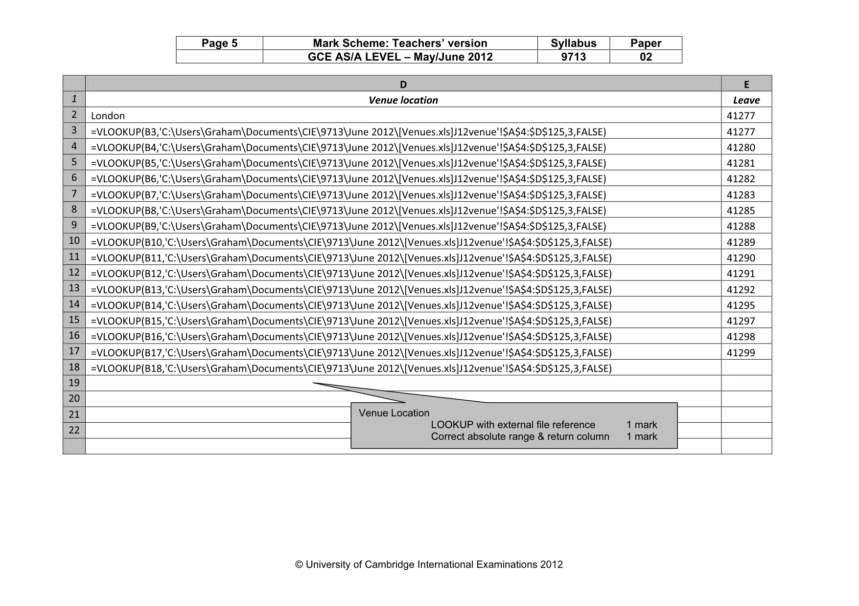
Page 5 Mark Scheme: Teachers’ version Syllabus Paper GCE AS/A LEVEL – May/June 2012 9713 02 © University of Cambridge International Examinations 2012 D E 1 Venue location Leave 2 London 41277 3 =VLOOKUP(B3,'C:\Users\Graham\Documents\CIE\9713\June 2012\[Venues.xls]J12venue'!$A$4:$D$125,3,FALSE) 41277 4 =VLOOKUP(B4,'C:\Users\Graham\Documents\CIE\9713\June 2012\[Venues.xls]J12venue'!$A$4:$D$125,3,FALSE) 41280 5 =VLOOKUP(B5,'C:\Users\Graham\Documents\CIE\9713\June 2012\[Venues.xls]J12venue'!$A$4:$D$125,3,FALSE) 41281 6 =VLOOKUP(B6,'C:\Users\Graham\Documents\CIE\9713\June 2012\[Venues.xls]J12venue'!$A$4:$D$125,3,FALSE) 41282 7 =VLOOKUP(B7,'C:\Users\Graham\Documents\CIE\9713\June 2012\[Venues.xls]J12venue'!$A$4:$D$125,3,FALSE) 41283 8 =VLOOKUP(B8,'C:\Users\Graham\Documents\CIE\9713\June 2012\[Venues.xls]J12venue'!$A$4:$D$125,3,FALSE) 41285 9 =VLOOKUP(B9,'C:\Users\Graham\Documents\CIE\9713\June 2012\[Venues.xls]J12venue'!$A$4:$D$125,3,FALSE) 41288 10 =VLOOKUP(B10,'C:\Users\Graham\Documents\CIE\9713\June 2012\[Venues.xls]J12venue'!$A$4:$D$125,3,FALSE) 41289 11 =VLOOKUP(B11,'C:\Users\Graham\Documents\CIE\9713\June 2012\[Venues.xls]J12venue'!$A$4:$D$125,3,FALSE) 41290 12 =VLOOKUP(B12,'C:\Users\Graham\Documents\CIE\9713\June 2012\[Venues.xls]J12venue'!$A$4:$D$125,3,FALSE) 41291 13 =VLOOKUP(B13,'C:\Users\Graham\Documents\CIE\9713\June 2012\[Venues.xls]J12venue'!$A$4:$D$125,3,FALSE) 41292 14 =VLOOKUP(B14,'C:\Users\Graham\Documents\CIE\9713\June 2012\[Venues.xls]J12venue'!$A$4:$D$125,3,FALSE) 41295 15 =VLOOKUP(B15,'C:\Users\Graham\Documents\CIE\9713\June 2012\[Venues.xls]J12venue'!$A$4:$D$125,3,FALSE) 41297 16 =VLOOKUP(B16,'C:\Users\Graham\Documents\CIE\9713\June 2012\[Venues.xls]J12venue'!$A$4:$D$125,3,FALSE) 41298 17 =VLOOKUP(B17,'C:\Users\Graham\Documents\CIE\9713\June 2012\[Venues.xls]J12venue'!$A$4:$D$125,3,FALSE) 41299 18 =VLOOKUP(B18,'C:\Users\Graham\Documents\CIE\9713\June 2012\[Venues.xls]J12venue'!$A$4:$D$125,3,FALSE) 19 20 21 22 Venue Location LOOKUP with external file reference 1 mark Correct absolute range & return column 1 mark
Mark scheme, page 6
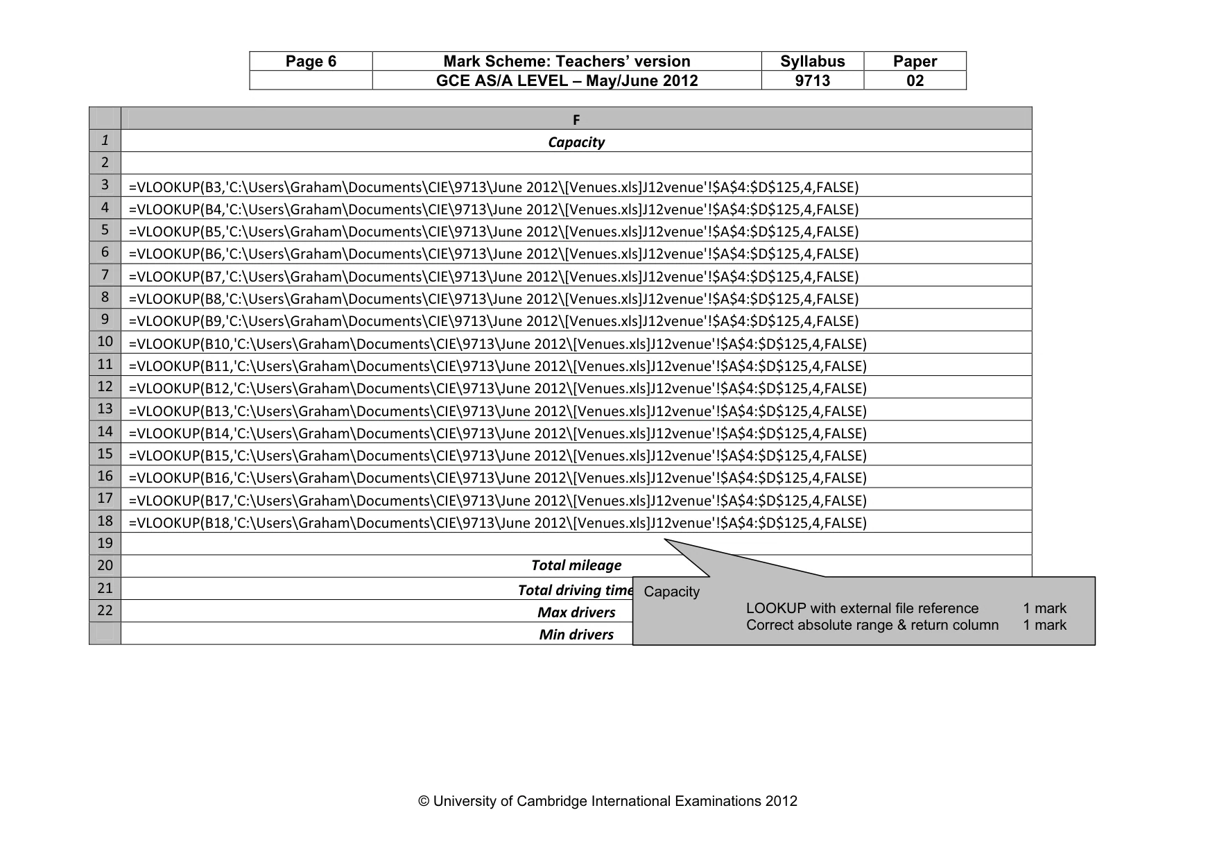
Page 6 Mark Scheme: Teachers’ version Syllabus Paper GCE AS/A LEVEL – May/June 2012 9713 02 © University of Cambridge International Examinations 2012 F 1 Capacity 2 3 =VLOOKUP(B3,'C:\Users\Graham\Documents\CIE\9713\June 2012\[Venues.xls]J12venue'!$A$4:$D$125,4,FALSE) 4 =VLOOKUP(B4,'C:\Users\Graham\Documents\CIE\9713\June 2012\[Venues.xls]J12venue'!$A$4:$D$125,4,FALSE) 5 =VLOOKUP(B5,'C:\Users\Graham\Documents\CIE\9713\June 2012\[Venues.xls]J12venue'!$A$4:$D$125,4,FALSE) 6 =VLOOKUP(B6,'C:\Users\Graham\Documents\CIE\9713\June 2012\[Venues.xls]J12venue'!$A$4:$D$125,4,FALSE) 7 =VLOOKUP(B7,'C:\Users\Graham\Documents\CIE\9713\June 2012\[Venues.xls]J12venue'!$A$4:$D$125,4,FALSE) 8 =VLOOKUP(B8,'C:\Users\Graham\Documents\CIE\9713\June 2012\[Venues.xls]J12venue'!$A$4:$D$125,4,FALSE) 9 =VLOOKUP(B9,'C:\Users\Graham\Documents\CIE\9713\June 2012\[Venues.xls]J12venue'!$A$4:$D$125,4,FALSE) 10 =VLOOKUP(B10,'C:\Users\Graham\Documents\CIE\9713\June 2012\[Venues.xls]J12venue'!$A$4:$D$125,4,FALSE) 11 =VLOOKUP(B11,'C:\Users\Graham\Documents\CIE\9713\June 2012\[Venues.xls]J12venue'!$A$4:$D$125,4,FALSE) 12 =VLOOKUP(B12,'C:\Users\Graham\Documents\CIE\9713\June 2012\[Venues.xls]J12venue'!$A$4:$D$125,4,FALSE) 13 =VLOOKUP(B13,'C:\Users\Graham\Documents\CIE\9713\June 2012\[Venues.xls]J12venue'!$A$4:$D$125,4,FALSE) 14 =VLOOKUP(B14,'C:\Users\Graham\Documents\CIE\9713\June 2012\[Venues.xls]J12venue'!$A$4:$D$125,4,FALSE) 15 =VLOOKUP(B15,'C:\Users\Graham\Documents\CIE\9713\June 2012\[Venues.xls]J12venue'!$A$4:$D$125,4,FALSE) 16 =VLOOKUP(B16,'C:\Users\Graham\Documents\CIE\9713\June 2012\[Venues.xls]J12venue'!$A$4:$D$125,4,FALSE) 17 =VLOOKUP(B17,'C:\Users\Graham\Documents\CIE\9713\June 2012\[Venues.xls]J12venue'!$A$4:$D$125,4,FALSE) 18 =VLOOKUP(B18,'C:\Users\Graham\Documents\CIE\9713\June 2012\[Venues.xls]J12venue'!$A$4:$D$125,4,FALSE) 19 20 Total mileage 21 Total driving time 22 Max drivers Min drivers Capacity LOOKUP with external file reference 1 mark Correct absolute range & return column 1 mark
Mark scheme, page 7
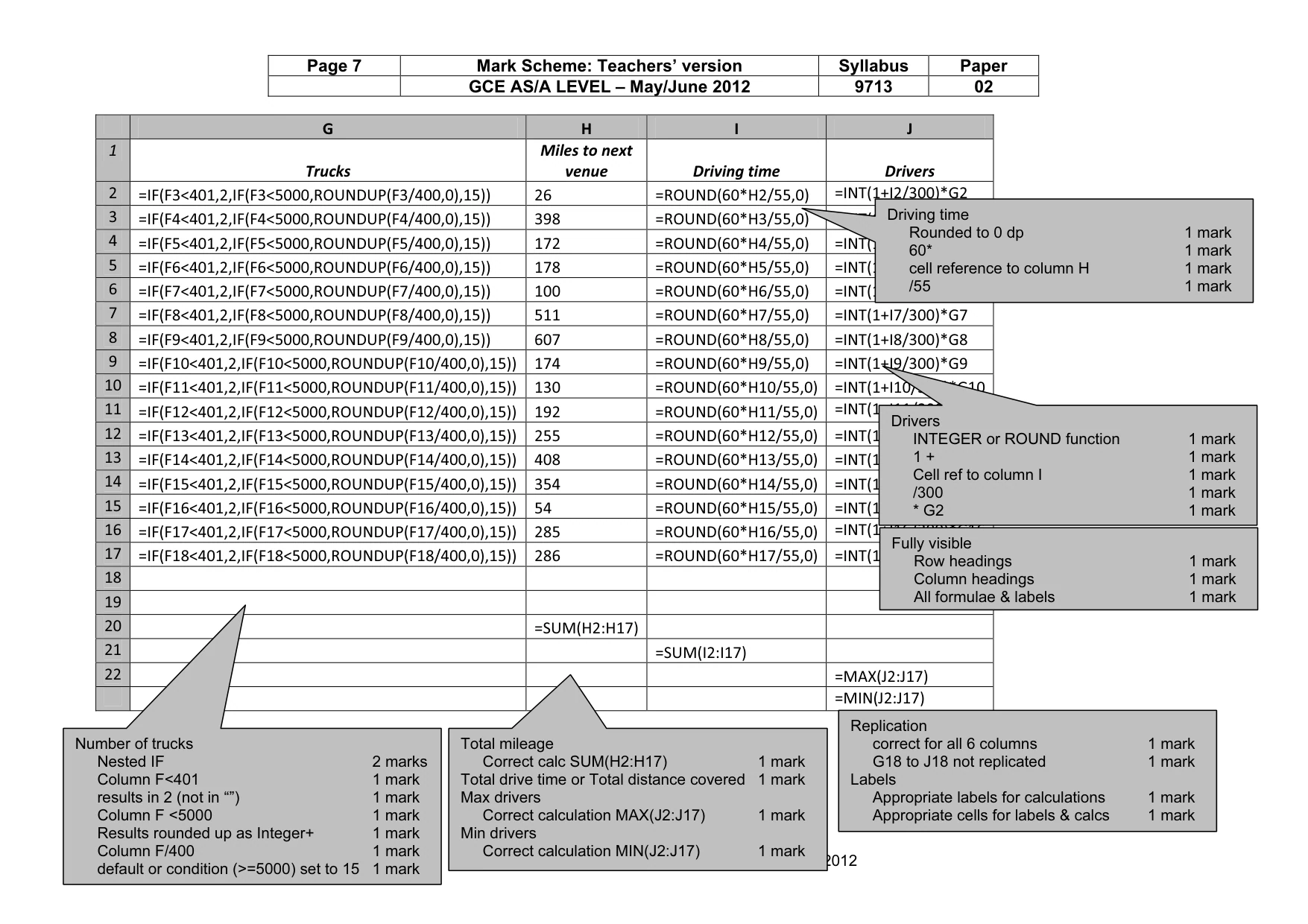
Page 7 Mark Scheme: Teachers’ version Syllabus Paper GCE AS/A LEVEL – May/June 2012 9713 02 © University of Cambridge International Examinations 2012 G H I J 1 Trucks Miles to next venue Driving time Drivers 2 =IF(F3<401,2,IF(F3<5000,ROUNDUP(F3/400,0),15)) 26 =ROUND(60*H2/55,0) =INT(1+I2/300)*G2 3 =IF(F4<401,2,IF(F4<5000,ROUNDUP(F4/400,0),15)) 398 =ROUND(60*H3/55,0) =INT(1+I3/300)*G3 4 =IF(F5<401,2,IF(F5<5000,ROUNDUP(F5/400,0),15)) 172 =ROUND(60*H4/55,0) =INT(1+I4/300)*G4 5 =IF(F6<401,2,IF(F6<5000,ROUNDUP(F6/400,0),15)) 178 =ROUND(60*H5/55,0) =INT(1+I5/300)*G5 6 =IF(F7<401,2,IF(F7<5000,ROUNDUP(F7/400,0),15)) 100 =ROUND(60*H6/55,0) =INT(1+I6/300)*G6 7 =IF(F8<401,2,IF(F8<5000,ROUNDUP(F8/400,0),15)) 511 =ROUND(60*H7/55,0) =INT(1+I7/300)*G7 8 =IF(F9<401,2,IF(F9<5000,ROUNDUP(F9/400,0),15)) 607 =ROUND(60*H8/55,0) =INT(1+I8/300)*G8 9 =IF(F10<401,2,IF(F10<5000,ROUNDUP(F10/400,0),15)) 174 =ROUND(60*H9/55,0) =INT(1+I9/300)*G9 10 =IF(F11<401,2,IF(F11<5000,ROUNDUP(F11/400,0),15)) 130 =ROUND(60*H10/55,0) =INT(1+I10/300)*G10 11 =IF(F12<401,2,IF(F12<5000,ROUNDUP(F12/400,0),15)) 192 =ROUND(60*H11/55,0) =INT(1+I11/300)*G11 12 =IF(F13<401,2,IF(F13<5000,ROUNDUP(F13/400,0),15)) 255 =ROUND(60*H12/55,0) =INT(1+I12/300)*G12 13 =IF(F14<401,2,IF(F14<5000,ROUNDUP(F14/400,0),15)) 408 =ROUND(60*H13/55,0) =INT(1+I13/300)*G13 14 =IF(F15<401,2,IF(F15<5000,ROUNDUP(F15/400,0),15)) 354 =ROUND(60*H14/55,0) =INT(1+I14/300)*G14 15 =IF(F16<401,2,IF(F16<5000,ROUNDUP(F16/400,0),15)) 54 =ROUND(60*H15/55,0) =INT(1+I15/300)*G15 16 =IF(F17<401,2,IF(F17<5000,ROUNDUP(F17/400,0),15)) 285 =ROUND(60*H16/55,0) =INT(1+I16/300)*G16 17 =IF(F18<401,2,IF(F18<5000,ROUNDUP(F18/400,0),15)) 286 =ROUND(60*H17/55,0) =INT(1+I17/300)*G17 18 19 20 =SUM(H2:H17) 21 =SUM(I2:I17) 22 =MAX(J2:J17) =MIN(J2:J17) Driving time Rounded to 0 dp 1 mark 60* 1 mark cell reference to column H 1 mark /55 1 mark Drivers INTEGER or ROUND function 1 mark 1 + 1 mark Cell ref to column I 1 mark /300 1 mark * G2 1 mark Fully visible Row headings 1 mark Column headings 1 mark All formulae & labels 1 mark Replication correct for all 6 columns 1 mark G18 to J18 not replicated 1 mark Labels Appropriate labels for calculations 1 mark Appropriate cells for labels & calcs 1 mark Total mileage Correct calc SUM(H2:H17) 1 mark Total drive time or Total distance covered 1 mark Max drivers Correct calculation MAX(J2:J17) 1 mark Min drivers Correct calculation MIN(J2:J17) 1 mark Number of trucks Nested IF 2 marks Column F<401 1 mark results in 2 (not in “”) 1 mark Column F <5000 1 mark Results rounded up as Integer+ 1 mark Column F/400 1 mark default or condition (>=5000) set to 15 1 mark
Mark scheme, page 8
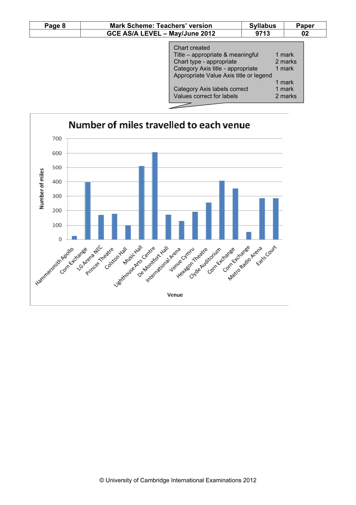
Page 8 Mark Scheme: Teachers’ version Syllabus Paper GCE AS/A LEVEL – May/June 2012 9713 02 © University of Cambridge International Examinations 2012 Chart created Title – appropriate & meaningful 1 mark Chart type - appropriate 2 marks Category Axis title - appropriate 1 mark Appropriate Value Axis title or legend 1 mark Category Axis labels correct 1 mark Values correct for labels 2 marks
Mark scheme, page 9
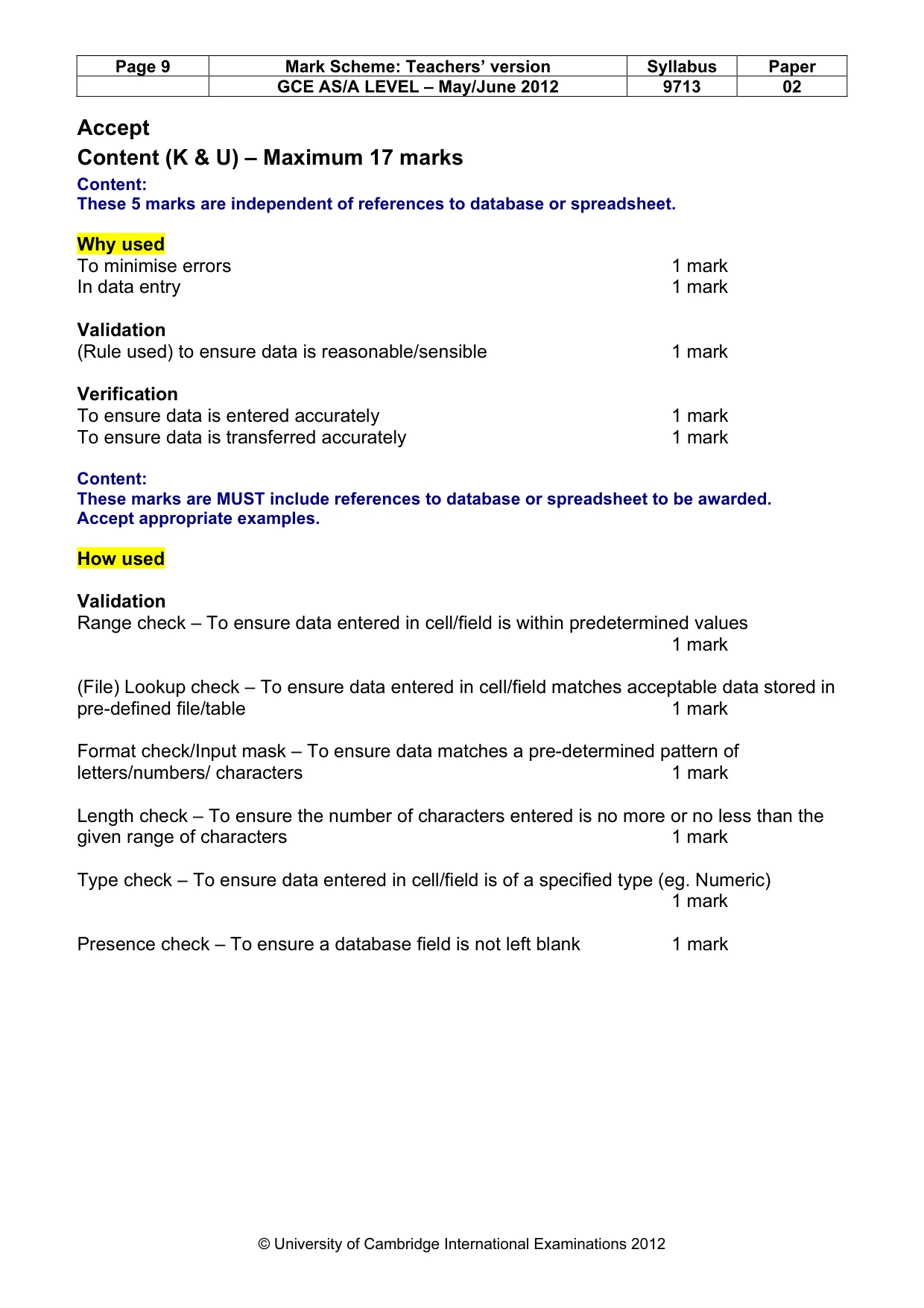
Page 9 Mark Scheme: Teachers’ version Syllabus Paper GCE AS/A LEVEL – May/June 2012 9713 02 © University of Cambridge International Examinations 2012 Accept Content (K & U) – Maximum 17 marks Content: These 5 marks are independent of references to database or spreadsheet. Why used To minimise errors 1 mark In data entry 1 mark Validation (Rule used) to ensure data is reasonable/sensible 1 mark Verification To ensure data is entered accurately 1 mark To ensure data is transferred accurately 1 mark Content: These marks are MUST include references to database or spreadsheet to be awarded. Accept appropriate examples. How used Validation Range check – To ensure data entered in cell/field is within predetermined values 1 mark (File) Lookup check – To ensure data entered in cell/field matches acceptable data stored in pre-defined file/table 1 mark Format check/Input mask – To ensure data matches a pre-determined pattern of letters/numbers/ characters 1 mark Length check – To ensure the number of characters entered is no more or no less than the given range of characters 1 mark Type check – To ensure data entered in cell/field is of a specified type (eg. Numeric) 1 mark Presence check – To ensure a database field is not left blank 1 mark
Mark scheme, page 10
Page 10 Mark Scheme: Teachers’ version Syllabus Paper GCE AS/A LEVEL – May/June 2012 9713 02 © University of Cambridge International Examinations 2012 Verification Visual verification Source document compared with data entered into cells of spreadsheet/database fields 2 marks Double entry (Database) table/transaction file/etc entered twice by different operators Compared by system/computer 2 marks Of transmitted data To check the contents of a file are not corrupted… …when being transmitted from one part of system to another/between computer systems 2 marks Max 17 marks
Mark scheme, page 11
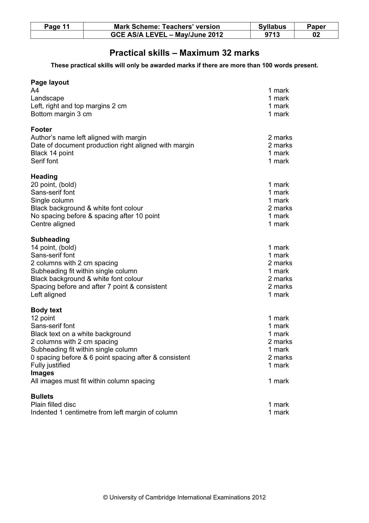
Page 11 Mark Scheme: Teachers’ version Syllabus Paper GCE AS/A LEVEL – May/June 2012 9713 02 © University of Cambridge International Examinations 2012 Practical skills – Maximum 32 marks These practical skills will only be awarded marks if there are more than 100 words present. Page layout A4 1 mark Landscape 1 mark Left, right and top margins 2 cm 1 mark Bottom margin 3 cm 1 mark Footer Author’s name left aligned with margin 2 marks Date of document production right aligned with margin 2 marks Black 14 point 1 mark Serif font 1 mark Heading 20 point, (bold) 1 mark Sans-serif font 1 mark Single column 1 mark Black background & white font colour 2 marks No spacing before & spacing after 10 point 1 mark Centre aligned 1 mark Subheading 14 point, (bold) 1 mark Sans-serif font 1 mark 2 columns with 2 cm spacing 2 marks Subheading fit within single column 1 mark Black background & white font colour 2 marks Spacing before and after 7 point & consistent 2 marks Left aligned 1 mark Body text 12 point 1 mark Sans-serif font 1 mark Black text on a white background 1 mark 2 columns with 2 cm spacing 2 marks Subheading fit within single column 1 mark 0 spacing before & 6 point spacing after & consistent 2 marks Fully justified 1 mark Images All images must fit within column spacing 1 mark Bullets Plain filled disc 1 mark Indented 1 centimetre from left margin of column 1 mark
Mark scheme, page 12
Page 12 Mark Scheme: Teachers’ version Syllabus Paper GCE AS/A LEVEL – May/June 2012 9713 02 © University of Cambridge International Examinations 2012 Presentation 4 slides and slide titles 1 mark Printed 4 per page 1 mark
Mark scheme, page 13
Page 13 Mark Scheme: Teachers’ version Syllabus Paper GCE AS/A LEVEL – May/June 2012 9713 02 © University of Cambridge International Examinations 2012 Menu options created for Band news & RockICT website 1 mark Image representing sending an email 1 mark Image set as hyperlink 1 mark Mailto:Lyryx@rockict.net 1 mark Subject line Lyryx Fan Club 1 mark Hyperlink from text RockICT website 1 mark To open the website http://www.rockict.net 1 mark Hyperlink from text Band news 1 mark To open the third slide 1 mark
What you needed in this session
Cambridge’s own grade thresholds for 2012 May/June, Paper 2 · Variant 1. A higher threshold means an easier paper — the bar moves with how the cohort did.