Questions as text
Q1 · A student is investigating how the discharge of a capacitor through a resistor depends on… 9702/53 Oct/Nov 2010
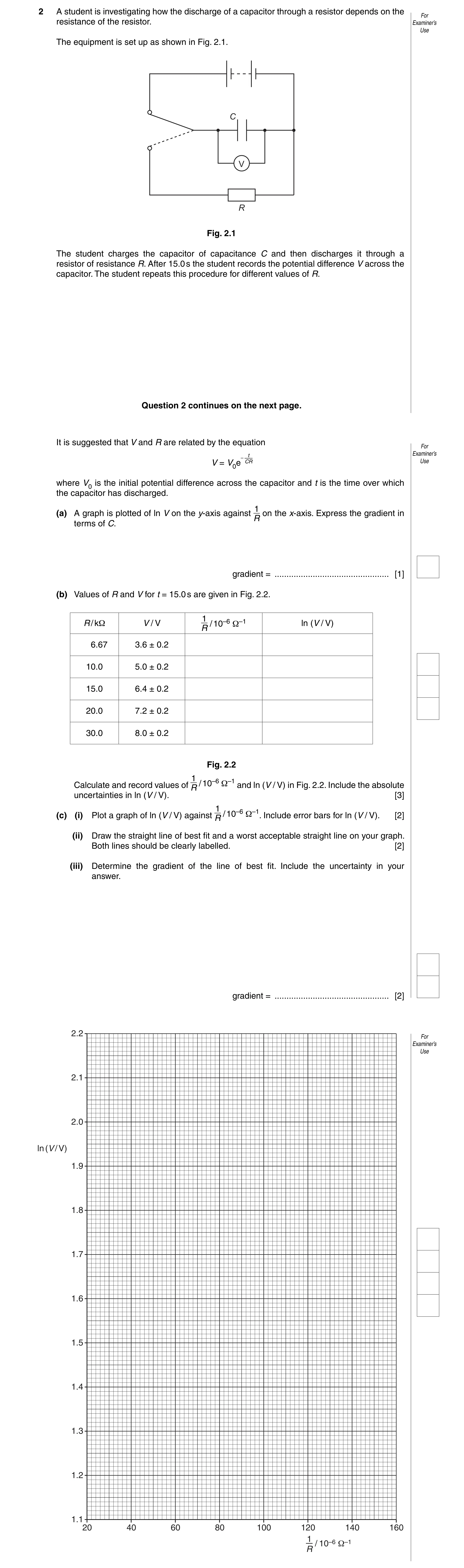
2 A student is investigating how the discharge of a capacitor through a resistor depends on the For resistance of the resistor. Examiner’s Use The equipment is set up as shown in Fig. 2.1. C V R Fig. 2.1 The student charges the capacitor of capacitance C and then discharges it through a resistor of resistance R. After 15.0 s the student records the potential difference V across the capacitor. The student repeats this procedure for different values of R. Question 2 continues on the next page. It is suggested that V and R are related by the equation For – t Examiner’s V = V0e CR Use where V0 is the initial potential difference across the capacitor and t is the time over which the capacitor has discharged. 1 (a) A graph is plotted of ln V on the y-axis against on the x-axis. Express the gradient in R terms of C. gradient = … [1] (b) Values of R and V for t = 15.0 s are given in Fig. 2.2. 1 R / kΩ V / V / 10–6 Ω–1 ln (V / V) R 6.67 3.6 ± 0.2 10.0 5.0 ± 0.2 15.0 6.4 ± 0.2 20.0 7.2 ± 0.2 30.0 8.0 ± 0.2 Fig. 2.2 1 Calculate and record values of / 10–6 Ω–1 and ln (V / V) in Fig. 2.2. Include the absolute R uncertainties in ln (V / V). [3] 1 (c) (i) Plot a graph of ln (V / V) against / 10–6 Ω–1. Include error bars for ln (V / V). [2] R (ii) Draw the straight line of best fit and a worst acceptable straight line on your graph. Both lines should be clearly labelled. [2] (iii) Determine the gradient of the line of best fit. Include the uncertainty in your answer. gradient = … [2] 2.2 For Examiner’s Use 2.1 2.0 ln (V / V) 1.9 1.8 1.7 1.6 1.5 1.4 1.3 1.2 1.1 20 40 60 80 100 120 140 160 / 10–6 Ω–1 1––R
10 marks
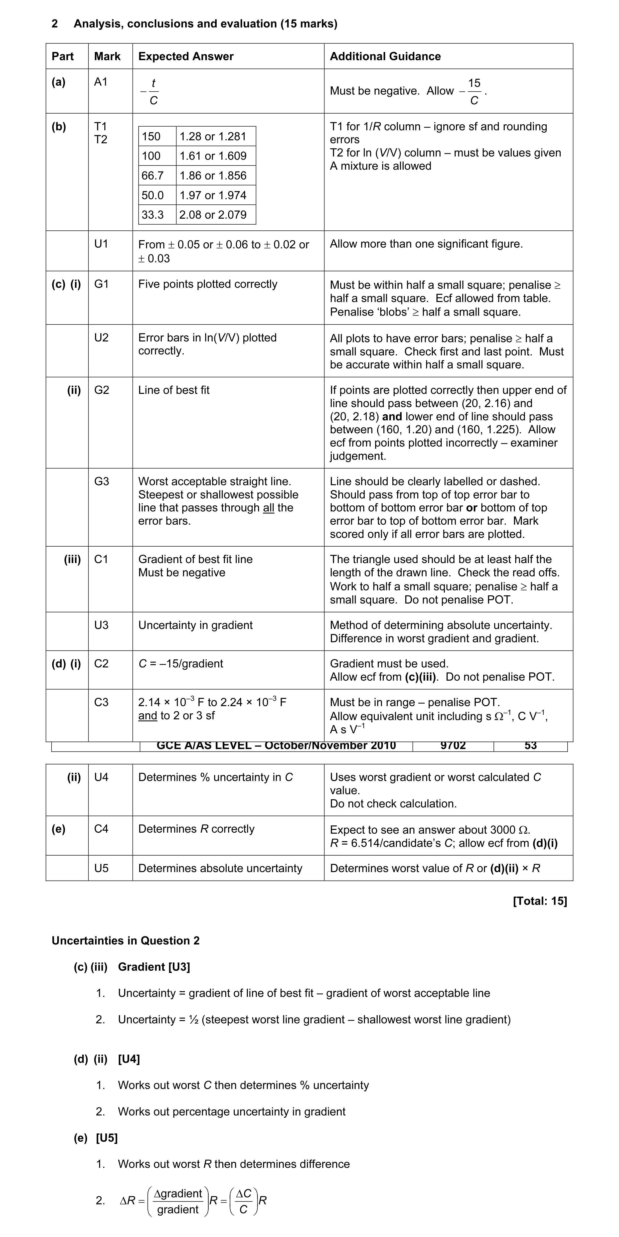
Mark scheme: 2 Analysis, conclusions and evaluation (15 marks) Part Mark Expected Answer Additional Guidance (a) A1 t 15 − Must be negative. Allow − . C C (b) T1 T1 for 1/R column – ignore sf and rounding T2 150 1.28 or 1.281 errors T2 for ln (V/V) column – must be values given 100 1.61 or 1.609 A mixture is allowed 66.7 1.86 or 1.856 50.0 1.97 or 1.974 33.3 2.08 or 2.079 U1 From ± 0.05 or ± 0.06 to ± 0.02 or Allow more than one significant figure. ± 0.03 (c) (i) G1 Five points plotted correctly Must be within half a small square; penalise ≥ half a small square. Ecf allowed from table. Penalise ‘blobs’ ≥ half a small square. U2 Error bars in ln(V/V) plotted All plots to have error bars; penalise ≥ half a correctly. small square. Check first and last point. Must be accurate within half a small square. (ii) G2 Line of best fit If points are plotted correctly then upper end of line should pass between (20, 2.16) and (20, 2.18) and lower end of line should pass between (160, 1.20) and (160, 1.225). Allow ecf from points plotted incorrectly – examiner judgement. G3 Worst acceptable straight line. Line should be clearly labelled or dashed. Steepest or shallowest possible Should pass from top of top error bar to line that passes through all the bottom of bottom error bar or bottom of top error bars. error bar to top of bottom error bar. Mark scored only if all error bars are plotted. (iii) C1 Gradient of best fit line The triangle used should be at least half the Must be negative length of the drawn line. Check the read offs. Work to half a small square; penalise ≥ half a small square. Do not penalise POT. U3 Uncertainty in gradient Method of determining absolute uncertainty. Difference in worst gradient and gradient. (d) (i) C2 C = –15/gradient Gradient must be used. Allow ecf from (c)(iii). Do not penalise POT. C3 2.14 × 10⁻³ F to 2.24 × 10⁻³ F Must be in range – penalise POT. and to 2 or 3 sf Allow equivalent unit including s Ω–1, C V–1, A s V–1 GCE A/AS LEVEL – October/November 2010 9702 53 (ii) U4 Determines % uncertainty in C Uses worst gradient or worst calculated C value. Do not check calculation. (e) C4 Determines R correctly Expect to see an answer about 3000 Ω. R = 6.514/candidate’s C; allow ecf from (d)(i) U5 Determines absolute uncertainty Determines worst value of R or (d)(ii) × R [Total: 15] Uncertainties in Question 2 (c) (iii) Gradient [U3] 1. Uncertainty = gradient of line of best fit – gradient of worst acceptable line 2. Uncertainty = ½ (steepest worst line gradient – shallowest worst line gradient) (d) (ii) [U4] 1. Works out worst C then determines % uncertainty 2. Works out percentage uncertainty in gradient (e) [U5] 1. Works out worst R then determines difference ∆gradient ∆C 2. ∆R = R = R gradient C
This question in 9702/53 Oct/Nov 2010
Q2 · A student is investigating the charging of a capacitor 9702/52 May/June 2018
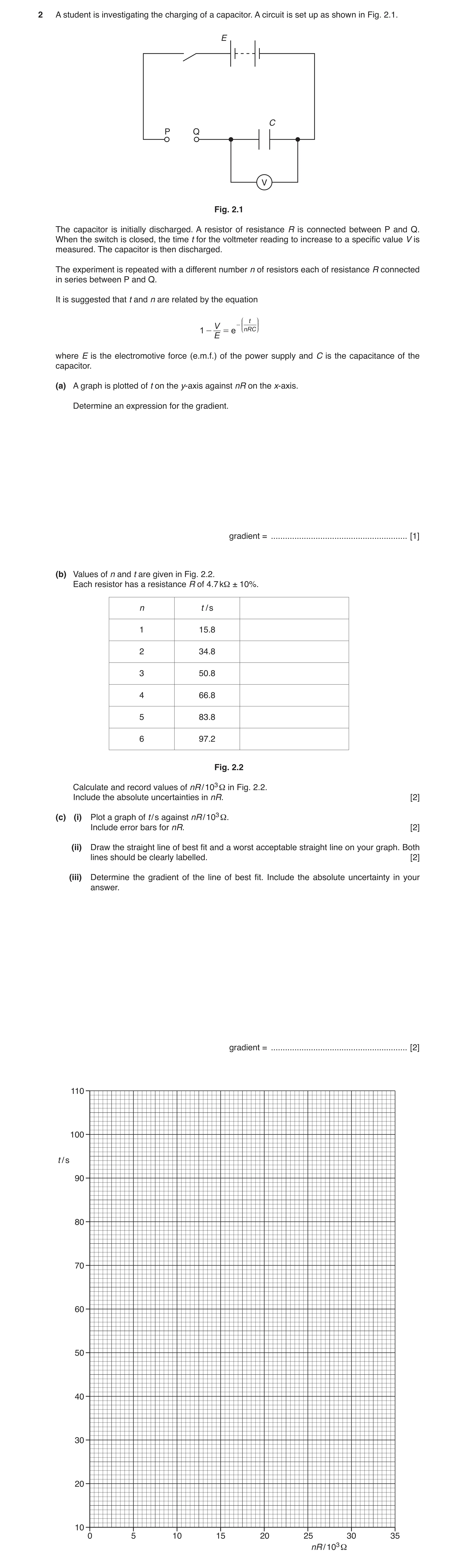
2 A student is investigating the charging of a capacitor. A circuit is set up as shown in Fig. 2.1. E C P Q V Fig. 2.1 The capacitor is initially discharged. A resistor of resistance R is connected between P and Q. When the switch is closed, the time t for the voltmeter reading to increase to a specific value V is measured. The capacitor is then discharged. The experiment is repeated with a different number n of resistors each of resistance R connected in series between P and Q. It is suggested that t and n are related by the equation J t N OO - KK V nRC L 1 - = e E P where E is the electromotive force (e.m.f.) of the power supply and C is the capacitance of the capacitor. (a) A graph is plotted of t on the y-axis against nR on the x-axis. Determine an expression for the gradient. gradient = … [1] (b) Values of n and t are given in Fig. 2.2. Each resistor has a resistance R of 4.7 kΩ ± 10%. n t / s 1 15.8 2 34.8 3 50.8 4 66.8 5 83.8 6 97.2 Fig. 2.2 Calculate and record values of nR / 103 Ω in Fig. 2.2. Include the absolute uncertainties in nR. [2] (c) (i) Plot a graph of t / s against nR / 103 Ω. Include error bars for nR. [2] (ii) Draw the straight line of best fit and a worst acceptable straight line on your graph. Both lines should be clearly labelled. [2] (iii) Determine the gradient of the line of best fit. Include the absolute uncertainty in your answer. gradient = … [2]
9 marks
Mark scheme: 2(a) gradient = ln 1 ln V E C C E E V − − − or 1 2(b) nR / 103 Ω absolute uncertainty in nR 4.7 or 4.70 0.5 or 0.47 9.4 or 9.40 0.9 or 0.94 14 or 14.1 1 or 1.4 or 1.41 19 or 18.8 2 or 1.9 or 1.88 24 or 23.5 2 or 2.4 or 2.35 28 or 28.2 3 or 2.8 or 2.82 First mark for correct column heading and values of nR. Second mark for absolute uncertainties in nR. Allow a mixture of significant figures. 2 2(c)(i) Six points plotted correctly. Must be within half a small square. Diameter of points must be less than half a small square. 1 Error bars in nR plotted correctly. All error bars to be plotted. Length of bar must be accurate to less than half a small square and symmetrical. 1 2(c)(ii) Line of best fit drawn. Upper end of line should pass between (25, 90) and (26, 90) and lower end of line should pass between (10.5, 40) and (11.5, 40). Do not allow line from top point to bottom point unless points are balanced. 1 Worst acceptable line drawn (steepest or shallowest possible line). All error bars must be plotted. 1 Question Answer Marks 2(c)(iii) Gradient determined with clear substitution of points from the line of best fit into ∆y / ∆x. Distance between points must be at least half the length of the drawn line. 1 Gradient of worst acceptable line determined. uncertainty = gradient of line of best fit – gradient of worst acceptable line or uncertainty = ½ (steepest worst line gradient – shallowest worst line gradient) 1 2(d)(i) C determined using gradient and given to 2 or 3 significant figures. 1 C determined using: ( ) gradient (c)(iii) (c)(iii) ln 0.2 1.609438 ln 1 C V E − − − = = = − − 1 C determined correctly using gradient and with unit (F or s Ω–1) and correct power of ten. 1 2(d)(ii) % uncertainty in C = % uncertainty in gradient. 1 Question Answer Marks 2(e) K determined using C. Correct substitution of numbers must be seen. ( ) 300 300 130.3 ln 1 0.9 2.30 (d)(i) (d)(i) K C − − = = = − × − × 1 Absolute uncertainty in K determined. Correct substitution of numbers must be seen. gradient uncertainty gradient C K K C ∆ ∆ = × = × Maximum/minimum methods: 130.3 130.3 1.609 209.69 max min (d)(i) min gradient min gradient K − − × − = = = 130.3 130.3 1.609 209.69 min max (d)(i) max gradient max gradient K − − × − = = = 1
This question in 9702/52 May/June 2018
Q3 · A student is investigating the behaviour of a capacitor-resistor circuit as shown in Fig 9702/52 Feb/March 2019
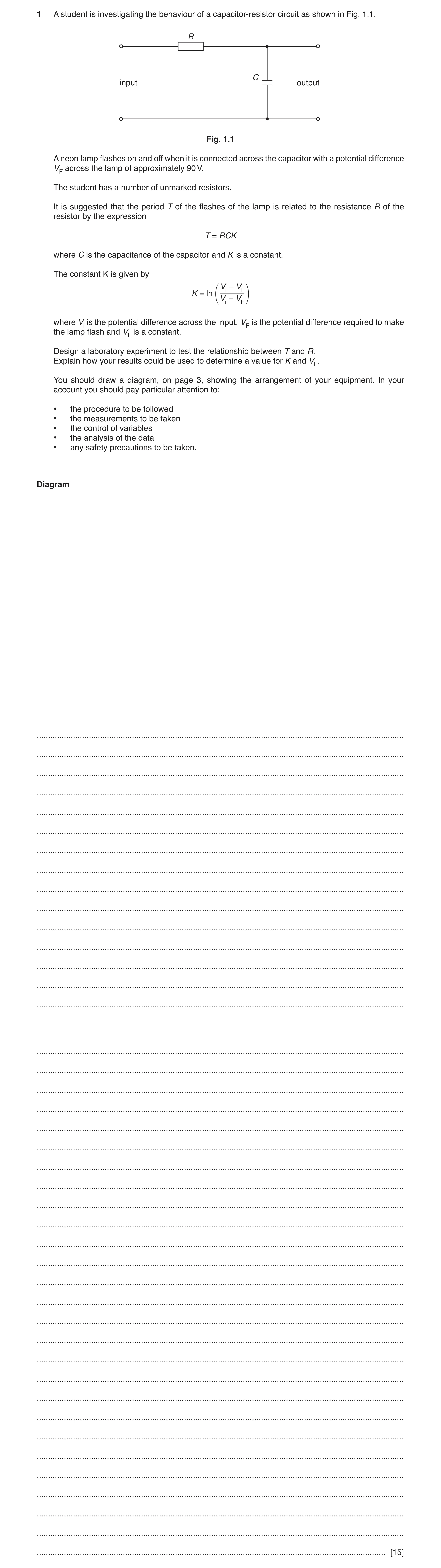
1 A student is investigating the behaviour of a capacitor-resistor circuit as shown in Fig. 1.1. R C input output Fig. 1.1 A neon lamp flashes on and off when it is connected across the capacitor with a potential difference VF across the lamp of approximately 90 V. The student has a number of unmarked resistors. It is suggested that the period T of the flashes of the lamp is related to the resistance R of the resistor by the expression T = RCK where C is the capacitance of the capacitor and K is a constant. The constant K is given by Vi – VL K = ln Vi – VF where Vi is the potential difference across the input, VF is the potential difference required to make the lamp flash and VL is a constant. Design a laboratory experiment to test the relationship between T and R. Explain how your results could be used to determine a value for K and VL. You should draw a diagram, on page 3, showing the arrangement of your equipment. In your account you should pay particular attention to: • the procedure to be followed • the measurements to be taken • the control of variables • the analysis of the data • any safety precautions to be taken. Diagram … … … … … … … … … … … … … … … … … … … … … … … … … … … … … … … … … … … … … … … … … … [15]
15 marks
Mark scheme: 1 Defining the problem R is the independent variable and T is the dependent variable, or vary R and measure T 1 keep C constant 1 Methods of data collection labelled diagram or correct symbols of workable circuit including: • (d.c.) power supply correctly positioned • (neon) lamp correctly positioned do not accept ohmmeter in circuit 1 circuit diagram to determine resistance of resistors e.g. using ammeter and voltmeter OR ohmmeter 1 method to determine period or T, e.g. use a stopwatch / timer / oscilloscope do not accept counting the flashes in a specified time 1 circuit diagram showing voltmeter(s) or oscilloscope(s) to determine Vi and VF 1 Method of Analysis plots a graph of T against R 1 gradient K C = 1 ( ) ( ) gradient K C L i i F i i F V V V V e V V V e = − − = − − 1 Question Answer Marks 1 Additional detail including safety considerations Max 6 switch off (high voltage) circuit (before changing the resistor) / wear insulating gloves to prevent electrocution / shock D1 resistance of resistors linked to diagram is V / I for ammeter / voltmeter method or gradient of appropriate graph or resistance from ohmmeter D2 input voltage or Vi is constant D3 repeat experiment for each value of R and average T D4 90 V (or larger) power supply do not accept a.c. or signal generator D5 for stopwatch method: time 10 or more flashes and divide by number of flashes for oscilloscope method: length of wave × timebase D6 record value of capacitance from the capacitor or method to determine capacitance D7 appropriate circuit to enable capacitance to be determined D8 relationship valid if a straight line passing through the origin is produced D9 method to obtain a measurable time period e.g. do a preliminary experiment to choose appropriate resistors, use large values of R or C D10
This question in 9702/52 Feb/March 2019
Q4 · A student investigates the discharge of a capacitor through a resistor as shown in Fig 9702/52 Feb/March 2020
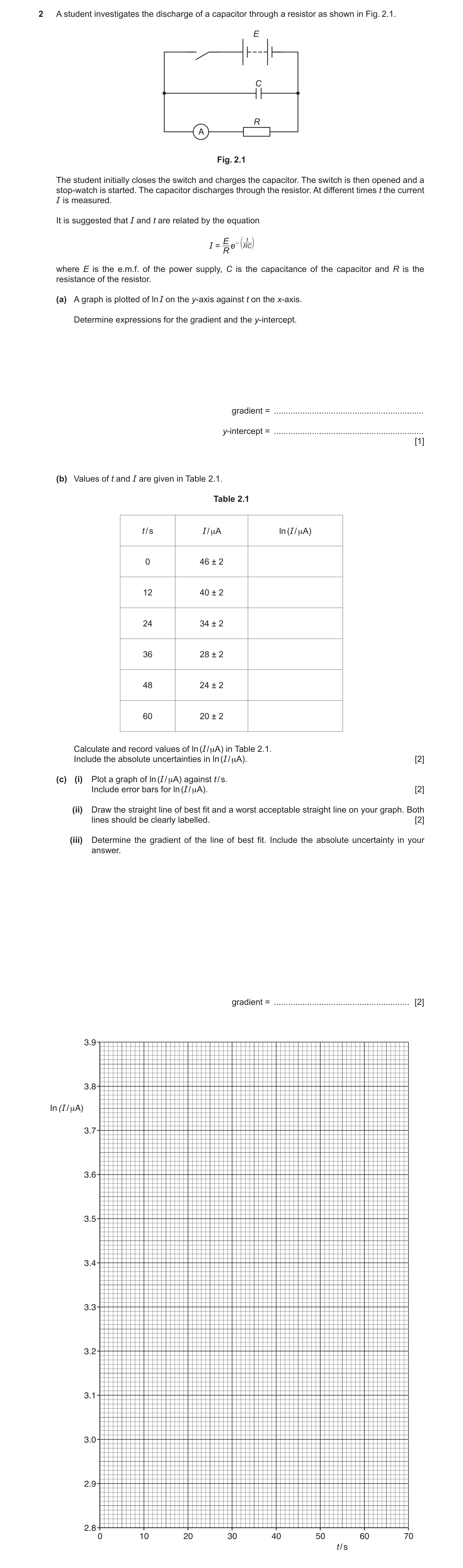
2 A student investigates the discharge of a capacitor through a resistor as shown in Fig. 2.1. E C R A Fig. 2.1 The student initially closes the switch and charges the capacitor. The switch is then opened and a stop-watch is started. The capacitor discharges through the resistor. At different times t the current I is measured. It is suggested that I and t are related by the equation E – t I = e e RC o R where E is the e.m.f. of the power supply, C is the capacitance of the capacitor and R is the resistance of the resistor. (a) A graph is plotted of ln I on the y-axis against t on the x-axis. Determine expressions for the gradient and the y-intercept. gradient = … y-intercept = … [1] (b) Values of t and I are given in Table 2.1. Table 2.1 t / s I / μA ln (I / μA) 0 46 ± 2 12 40 ± 2 24 34 ± 2 36 28 ± 2 48 24 ± 2 60 20 ± 2 Calculate and record values of ln (I / μA) in Table 2.1. Include the absolute uncertainties in ln (I / μA). [2] (c) (i) Plot a graph of ln (I / μA) against t / s. Include error bars for ln (I / μA). [2] (ii) Draw the straight line of best fit and a worst acceptable straight line on your graph. Both lines should be clearly labelled. [2] (iii) Determine the gradient of the line of best fit. Include the absolute uncertainty in your answer. gradient = … [2]
9 marks
Mark scheme: 2(a) Gradient = −1 CR y-intercept = ln E R 2(b) 3.83 or 3.829 3.69 or 3.689 3.53 or 3.526 3.33 or 3.332 3.18 or 3.178 3.00 or 2.996 1 Absolute uncertainties in ln I from ± 0.04 to ± 0.1 1 2(c)(i) Six points plotted correctly. Must be within half a small square. Diameter of points must be less than half a small square. 1 Error bars in ln I plotted correctly. All error bars to be plotted. Total length of bar must be accurate to less than half a small square and symmetrical. 1 2(c)(ii) Line of best fit drawn. Points must be balanced. Line must pass between (5.5, 3.75) and (8.0, 3.75) and between (56, 3.05) and (58, 3.05) 1 Worst acceptable line drawn. Steepest or shallowest possible line that passes through all the error bars. Mark scored only if all error bars are plotted. 1 Question Answer Marks 2(c)(iii) Negative gradient determined with clear substitution of data points into Δy / Δx; distance between data points must be at least half the length of the drawn line. 1 Gradient determined of WAL uncertainty = (gradient of line of best fit – gradient of worst acceptable line) or uncertainty = ½ (steepest worst line gradient – shallowest worst line gradient) 1 2(c)(iv) y-intercept read from y-axis to less than half a small square, or y-intercept determined from substitution into y = m x + c. 1 2(d)(i) C determined using gradient and C given to two or three significant figures Correct substitution of numbers must be seen, − − = = × × × × 3 3 1 1 150 10 gradient 150 10 (c)(iii) C 1 E determined using y-intercept Correct substitution of numbers must be seen, ( ) − = × = × × × -intercept 3 (c)(iv) 6 150 10 e 10 y E R e Or = + ln ln -intercept E R y 1 C determined using gradient and E determined using y-intercept and dimensionally correct SI unit for C: F or s Ω–1 or C V–1 or A s V–1 and E: V or A Ω. 1 Question Answer Marks 2(d)(ii) Absolute uncertainty in C. Δ Δ = + × gradient 0.05 gradient C C OR Correct substitution for max/min methods − = × × 3 1 max 142.5 10 minnumericalgradient C − = × × 3 1 min 157.5 10 max numerical gradient C 1 2(e) I determined from (d)(i) OR (c)(iii) and (c)(iv) with correct substitution and correct power of ten(s). Do not accept ecf for POT from (c)(iii), (iv) or (d). − = × 120 CR E e R I OR ( ) × − = × × gradient 120 -intercept 6 10 y e e I OR = × + ln 120 gradient -intercept y I × + − = × 120 gradient -intercept 6 10 y e I 1
This question in 9702/52 Feb/March 2020
Q5 · A student investigates the discharge of a capacitor through a resistor using the circuit… 9702/51 May/June 2020
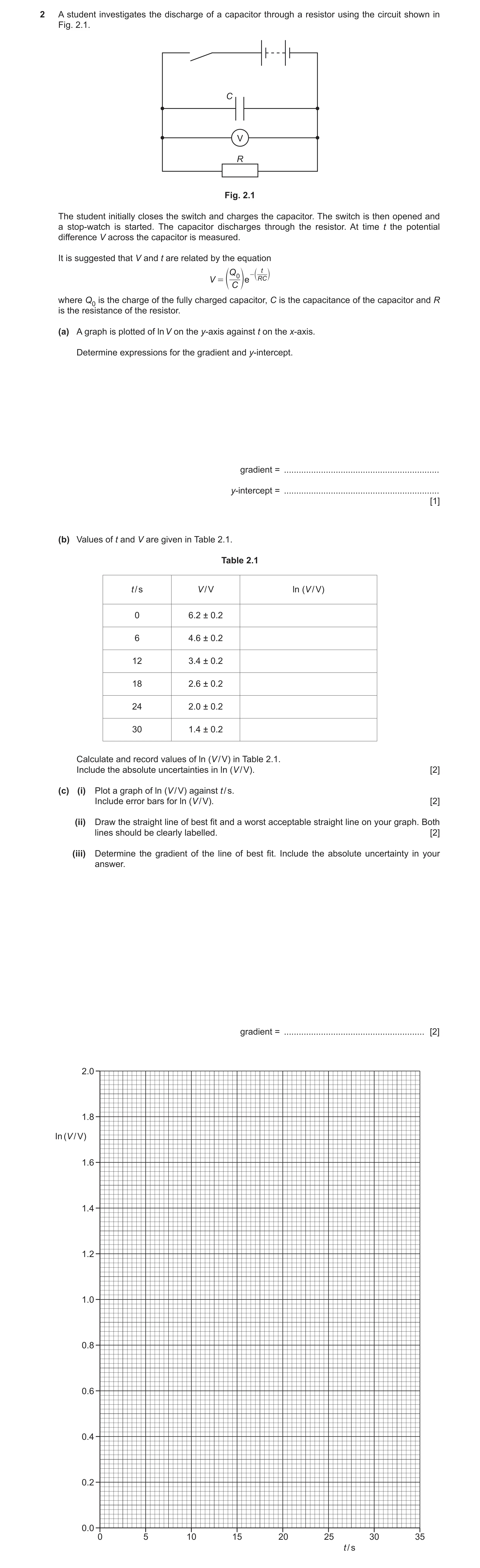
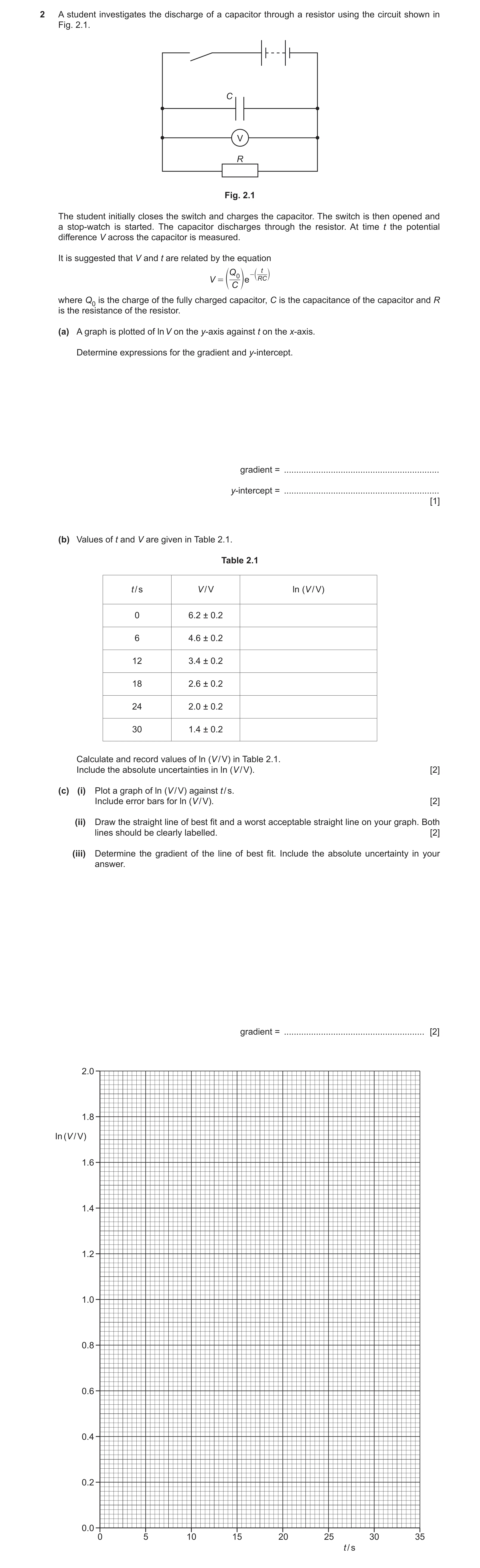
2 A student investigates the discharge of a capacitor through a resistor using the circuit shown in Fig. 2.1. C V R Fig. 2.1 The student initially closes the switch and charges the capacitor. The switch is then opened and a stop-watch is started. The capacitor discharges through the resistor. At time t the potential difference V across the capacitor is measured. It is suggested that V and t are related by the equation t 0 c RC m e - V = o e QC where Q0 is the charge of the fully charged capacitor, C is the capacitance of the capacitor and R is the resistance of the resistor. (a) A graph is plotted of ln V on the y-axis against t on the x-axis. Determine expressions for the gradient and y-intercept. gradient = … y-intercept = … [1] (b) Values of t and V are given in Table 2.1. Table 2.1 t / s V / V ln (V / V) 0 6.2 ± 0.2 6 4.6 ± 0.2 12 3.4 ± 0.2 18 2.6 ± 0.2 24 2.0 ± 0.2 30 1.4 ± 0.2 Calculate and record values of ln (V / V) in Table 2.1. Include the absolute uncertainties in ln (V / V). [2] (c) (i) Plot a graph of ln (V / V) against t / s. Include error bars for ln (V / V). [2] (ii) Draw the straight line of best fit and a worst acceptable straight line on your graph. Both lines should be clearly labelled. [2] (iii) Determine the gradient of the line of best fit. Include the absolute uncertainty in your answer. gradient = … [2]
9 marks
Mark scheme: 2(a) gradient = 1 CR − y-intercept = ln 0 Q C 1 2(b) ln (V / V) 1.82 or 1.825 1.53 or 1.526 1.22 or 1.224 0.96 or 0.956 0.69 or 0.693 0.34 or 0.336 1 Absolute uncertainties in ln V from ± 0.03 or ± 0.04 to ± 0.13 or ± 0.14 or ± 0.15. 1 2(c)(i) Six points plotted correctly. Must be within half a small square. Diameter of points must be less than half a small square. 1 Error bars in ln V plotted correctly. All error bars to be plotted. Length of bar must be accurate to less than half a small square and symmetrical. 1 2(c)(ii) Line of best fit drawn. Points must be balanced. Do not accept top point to bottom point. Line must pass between (4.0, 1.6) and (5.0, 1.6) and between (26.5, 0.5) and (28.0, 0.5) 1 Worst acceptable line drawn (steepest or shallowest possible line that passes through all the error bars). All error bars must be plotted. 1 Question Answer Marks 2(c)(iii) Gradient determined with clear substitution of data points into Δy / Δx. Distance between data points must be at least half the length of the drawn line. Gradient must be negative. 1 uncertainty = (gradient of line of best fit – gradient of worst acceptable line) or uncertainty = ½ (steepest worst line gradient – shallowest worst line gradient) 1 2(c)(iv) y-intercept read from y-axis to less than half a small square or y-intercept determined from substitution into y = mx + c. 1 2(d)(i) C determined using gradient and C and Q0 given to two or three significant figures. Correct substitution of numbers required. 3 3 1 1 39 10 gradient 39 10 C − − = = × × × × (c)(iii) 1 Q0 determined using y-intercept. -intercept 0 y Q C e C e = × = × (c)(iv) 1 C determined using gradient and Q0 determined using y-intercept and dimensionally correct units for C (F or s Ω–1) and Q0 (C or V s Ω–1 or A s). 1 2(d)(ii) Absolute uncertainty in C. gradient 0.05 gradient C C Δ Δ = + × 1 Question Answer Marks 2(e) V determined from (d)(i) (or (c)(iii) and (c)(iv)) with correct substitution shown and correct power of ten. ( ) 60 gradient 60 -intercept 0 y CR Q V e e e C − × = × = × or ln V = – (t / RC) + ln (Q0 / C) = – (60 / 39 000) × (d)(i) + ln (Q0 / C) ln V = 60 × gradient + y-intercept ln V = 60 × (c)(iii) + (c)(iv) 1
This question in 9702/51 May/June 2020
Q6 · A student investigates the discharge of a capacitor through a resistor using the circuit… 9702/53 May/June 2020
2 A student investigates the discharge of a capacitor through a resistor using the circuit shown in Fig. 2.1. C V R Fig. 2.1 The student initially closes the switch and charges the capacitor. The switch is then opened and a stop-watch is started. The capacitor discharges through the resistor. At time t the potential difference V across the capacitor is measured. It is suggested that V and t are related by the equation t 0 c RC m e - V = o e QC where Q0 is the charge of the fully charged capacitor, C is the capacitance of the capacitor and R is the resistance of the resistor. (a) A graph is plotted of ln V on the y-axis against t on the x-axis. Determine expressions for the gradient and y-intercept. gradient = … y-intercept = … [1] (b) Values of t and V are given in Table 2.1. Table 2.1 t / s V / V ln (V / V) 0 6.2 ± 0.2 6 4.6 ± 0.2 12 3.4 ± 0.2 18 2.6 ± 0.2 24 2.0 ± 0.2 30 1.4 ± 0.2 Calculate and record values of ln (V / V) in Table 2.1. Include the absolute uncertainties in ln (V / V). [2] (c) (i) Plot a graph of ln (V / V) against t / s. Include error bars for ln (V / V). [2] (ii) Draw the straight line of best fit and a worst acceptable straight line on your graph. Both lines should be clearly labelled. [2] (iii) Determine the gradient of the line of best fit. Include the absolute uncertainty in your answer. gradient = … [2]
9 marks
Mark scheme: 2(a) gradient = 1 CR − y-intercept = ln 0 Q C 1 2(b) ln (V / V) 1.82 or 1.825 1.53 or 1.526 1.22 or 1.224 0.96 or 0.956 0.69 or 0.693 0.34 or 0.336 1 Absolute uncertainties in ln V from ± 0.03 or ± 0.04 to ± 0.13 or ± 0.14 or ± 0.15. 1 2(c)(i) Six points plotted correctly. Must be within half a small square. Diameter of points must be less than half a small square. 1 Error bars in ln V plotted correctly. All error bars to be plotted. Length of bar must be accurate to less than half a small square and symmetrical. 1 2(c)(ii) Line of best fit drawn. Points must be balanced. Do not accept top point to bottom point. Line must pass between (4.0, 1.6) and (5.0, 1.6) and between (26.5, 0.5) and (28.0, 0.5) 1 Worst acceptable line drawn (steepest or shallowest possible line that passes through all the error bars). All error bars must be plotted. 1 Question Answer Marks 2(c)(iii) Gradient determined with clear substitution of data points into Δy / Δx. Distance between data points must be at least half the length of the drawn line. Gradient must be negative. 1 uncertainty = (gradient of line of best fit – gradient of worst acceptable line) or uncertainty = ½ (steepest worst line gradient – shallowest worst line gradient) 1 2(c)(iv) y-intercept read from y-axis to less than half a small square or y-intercept determined from substitution into y = mx + c. 1 2(d)(i) C determined using gradient and C and Q0 given to two or three significant figures. Correct substitution of numbers required. 3 3 1 1 39 10 gradient 39 10 C − − = = × × × × (c)(iii) 1 Q0 determined using y-intercept. -intercept 0 y Q C e C e = × = × (c)(iv) 1 C determined using gradient and Q0 determined using y-intercept and dimensionally correct units for C (F or s Ω–1) and Q0 (C or V s Ω–1 or A s). 1 2(d)(ii) Absolute uncertainty in C. gradient 0.05 gradient C C Δ Δ = + × 1 Question Answer Marks 2(e) V determined from (d)(i) (or (c)(iii) and (c)(iv)) with correct substitution shown and correct power of ten. ( ) 60 gradient 60 -intercept 0 y CR Q V e e e C − × = × = × or ln V = – (t / RC) + ln (Q0 / C) = – (60 / 39 000) × (d)(i) + ln (Q0 / C) ln V = 60 × gradient + y-intercept ln V = 60 × (c)(iii) + (c)(iv) 1
This question in 9702/53 May/June 2020
Q7 · A student investigates the discharge of a capacitor in the circuit shown in Fig 9702/51 Oct/Nov 2021
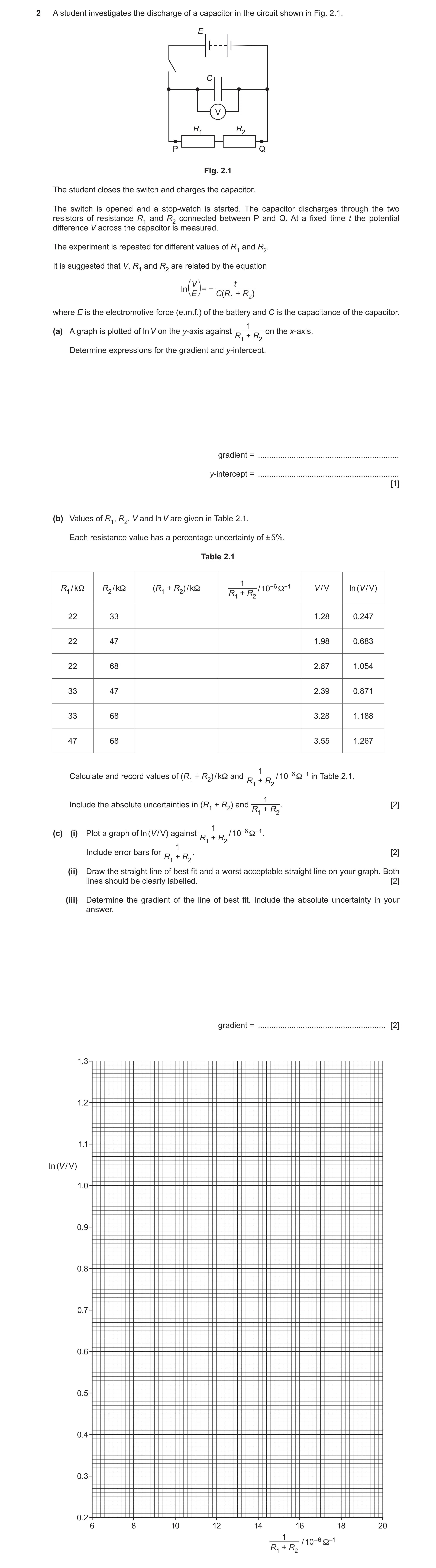
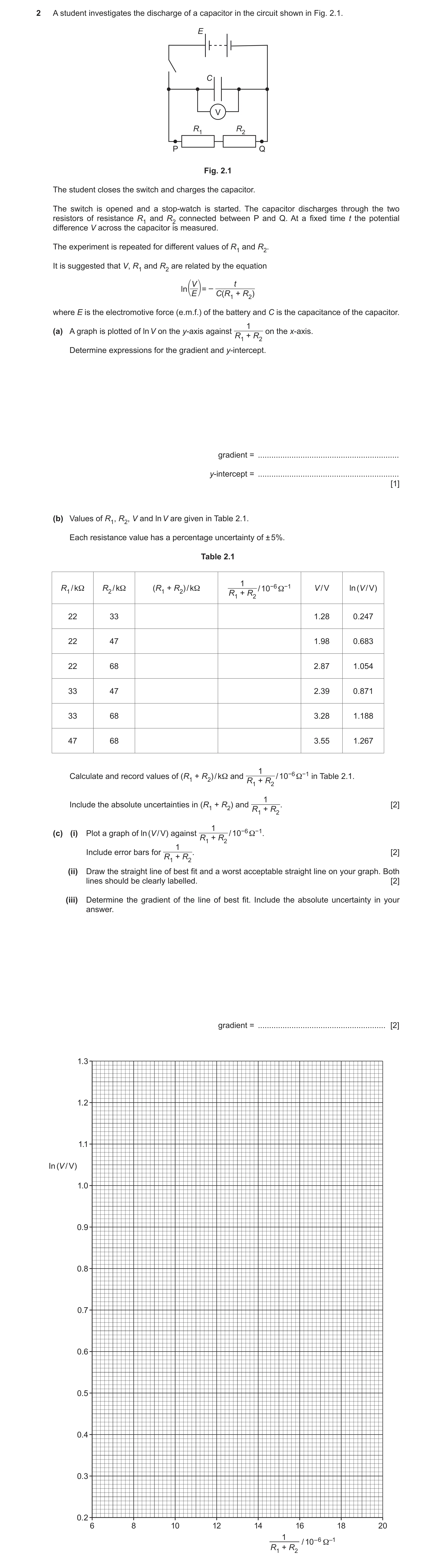
2 A student investigates the discharge of a capacitor in the circuit shown in Fig. 2.1. E C V R1 R2 P Q Fig. 2.1 The student closes the switch and charges the capacitor. The switch is opened and a stop-watch is started. The capacitor discharges through the two resistors of resistance R1 and R2 connected between P and Q. At a fixed time t the potential difference V across the capacitor is measured. The experiment is repeated for different values of R1 and R2. It is suggested that V, R1 and R2 are related by the equation ⎛⎞V t ln = – ⎝⎠E C(R1 + R2) where E is the electromotive force (e.m.f.) of the battery and C is the capacitance of the capacitor. 1 (a) A graph is plotted of ln V on the y-axis against on the x-axis. R1 + R2 Determine expressions for the gradient and y-intercept. gradient = … y-intercept = … [1] (b) Values of R1, R2, V and ln V are given in Table 2.1. Each resistance value has a percentage uncertainty of ± 5%. Table 2.1 1 R1 / kΩ R2 / kΩ (R1 + R2) / kΩ / 10−6 Ω−1 V / V ln (V / V) R1 + R2 22 33 1.28 0.247 22 47 1.98 0.683 22 68 2.87 1.054 33 47 2.39 0.871 33 68 3.28 1.188 47 68 3.55 1.267 1 Calculate and record values of (R1 + R2) / kΩ and / 10−6 Ω−1 in Table 2.1. R1 + R2 1 Include the absolute uncertainties in (R1 + R2) and . [2] R1 + R2 1(c) (i) Plot a graph of ln (V / V) against / 10−6 Ω−1. R1 + R2 1 Include error bars for . [2] R1 + R2 (ii) Draw the straight line of best fit and a worst acceptable straight line on your graph. Both lines should be clearly labelled. [2] (iii) Determine the gradient of the line of best fit. Include the absolute uncertainty in your answer. gradient = … [2]
9 marks
Mark scheme: 2(a) gradient = – t C y-intercept = ln E 1 2(b) (R1 + R2) / kΩ 1 2 1 R R + / 10–6 Ω 55 (± 3) 18 or 18.2 ± 0.9 69 (± 3 or 4) 14 or 14.5 ± 0.7 90 (± 4 or 5) 11 or 11.1 ± 0.6 80 (± 4) 13 or 12.5 ± 0.6 101 (± 5) 9.9 or 9.90 or 9.901 ± 0.5 115 (± 6) 8.7 or 8.70 or 8.696 ± 0.4 Values of (R1 + R2) and 1 2 1 R R + correct as shown above. 1 Absolute uncertainties in 1 2 1 R R + from ± 0.9 or ± 1 to ± 0.4 or ± 0.5. 1 2(c)(i) Six points plotted correctly. Must be accurate to half a small square. Diameter of points must be less than half a small square. 1 Error bars in 1 2 1 R R + plotted correctly. All error bars must be plotted. Total length of bar must be accurate to less than half a small square and symmetrical. 1 Question Answer Marks 2(c)(ii) Line of best fit drawn. Points must be balanced. Do not accept line from top point to bottom point. Line must pass between (10.2, 1.10) and (10.8, 1.10) and between (16.7, 0.40) and (17.2, 0.40). 1 Worst acceptable line drawn (steepest or shallowest possible line that passes through all error bars). All error bars must be plotted. 1 2(c)(iii) Negative gradient determined with clear substitution of data points into Δy / Δx. Distance between data points must be at least half the length of the drawn line. 1 Gradient of worst acceptable line determined. uncertainty = (gradient of line of best fit – gradient of worst acceptable line) or uncertainty = ½ (steepest worst line gradient – shallowest worst line gradient) 1 2(c)(iv) y-intercept determined by substitution of point on line into y = mx + c. 1 y-intercept of worst acceptable line determined by substitution of point on line into y = mx + c. uncertainty = y-intercept of line of best fit – y-intercept of worst acceptable line or uncertainty = ½ (steepest worst line y-intercept – shallowest worst line y-intercept) Do not accept ECF from false origin method. 1 2(d)(i) C determined using gradient and C and E both given to two or three significant figures. 60 gradient t C = − = −(c)(iii) 1 E determined using y-intercept and C and E both given with correct SI unit. = -intercept ey E unit of C: F or C V–1 or s Ω–1 unit of E: V 1 Question Answer Marks 2(d)(ii) Percentage uncertainty determined with method shown. Δ = + × 1 gradient percentage uncertainty 100 60 gradient Clear substitution must be shown for maximum/minimum methods. 1 2(e) (R1 + R2) determined to at least two significant figures from (d)(i) or (c)(iii) and (c)(iv) with correct substitution including signs and correct power of ten(s). Do not accept ECF for POT from (c)(iii), (c)(iv) or (d). ( ) 1 2 1 60 1 ln ln ln t R R V C C V E E + = − × = − × − or ( ) + = = − − 1 2 gradient ln5.0 -intercept 1.61 R R y (c)(iii) (c)(iv) 1
This question in 9702/51 Oct/Nov 2021
Q8 · A student investigates the discharge of a capacitor in the circuit shown in Fig 9702/53 Oct/Nov 2021
2 A student investigates the discharge of a capacitor in the circuit shown in Fig. 2.1. E C V R1 R2 P Q Fig. 2.1 The student closes the switch and charges the capacitor. The switch is opened and a stop-watch is started. The capacitor discharges through the two resistors of resistance R1 and R2 connected between P and Q. At a fixed time t the potential difference V across the capacitor is measured. The experiment is repeated for different values of R1 and R2. It is suggested that V, R1 and R2 are related by the equation ⎛⎞V t ln = – ⎝⎠E C(R1 + R2) where E is the electromotive force (e.m.f.) of the battery and C is the capacitance of the capacitor. 1 (a) A graph is plotted of ln V on the y-axis against on the x-axis. R1 + R2 Determine expressions for the gradient and y-intercept. gradient = … y-intercept = … [1] (b) Values of R1, R2, V and ln V are given in Table 2.1. Each resistance value has a percentage uncertainty of ± 5%. Table 2.1 1 R1 / kΩ R2 / kΩ (R1 + R2) / kΩ / 10−6 Ω−1 V / V ln (V / V) R1 + R2 22 33 1.28 0.247 22 47 1.98 0.683 22 68 2.87 1.054 33 47 2.39 0.871 33 68 3.28 1.188 47 68 3.55 1.267 1 Calculate and record values of (R1 + R2) / kΩ and / 10−6 Ω−1 in Table 2.1. R1 + R2 1 Include the absolute uncertainties in (R1 + R2) and . [2] R1 + R2 1(c) (i) Plot a graph of ln (V / V) against / 10−6 Ω−1. R1 + R2 1 Include error bars for . [2] R1 + R2 (ii) Draw the straight line of best fit and a worst acceptable straight line on your graph. Both lines should be clearly labelled. [2] (iii) Determine the gradient of the line of best fit. Include the absolute uncertainty in your answer. gradient = … [2]
9 marks
Mark scheme: 2(a) gradient = – t C y-intercept = ln E 2(b) (R1 + R2) / kΩ 1 2 1 R R + / 10–6 Ω 55 (± 3) 18 or 18.2 ± 0.9 69 (± 3 or 4) 14 or 14.5 ± 0.7 90 (± 4 or 5) 11 or 11.1 ± 0.6 80 (± 4) 13 or 12.5 ± 0.6 101 (± 5) 9.9 or 9.90 or 9.901 ± 0.5 115 (± 6) 8.7 or 8.70 or 8.696 ± 0.4 Values of (R1 + R2) and 1 2 1 R R + correct as shown above. 1 Absolute uncertainties in 1 2 1 R R + from ± 0.9 or ± 1 to ± 0.4 or ± 0.5. 1 2(c)(i) Six points plotted correctly. Must be accurate to half a small square. Diameter of points must be less than half a small square. 1 Error bars in 1 2 1 R R + plotted correctly. All error bars must be plotted. Total length of bar must be accurate to less than half a small square and symmetrical. 1 Question Answer Marks 2(c)(ii) Line of best fit drawn. Points must be balanced. Do not accept line from top point to bottom point. Line must pass between (10.2, 1.10) and (10.8, 1.10) and between (16.7, 0.40) and (17.2, 0.40). 1 Worst acceptable line drawn (steepest or shallowest possible line that passes through all error bars). All error bars must be plotted. 1 2(c)(iii) Negative gradient determined with clear substitution of data points into Δy / Δx. Distance between data points must be at least half the length of the drawn line. 1 Gradient of worst acceptable line determined. uncertainty = (gradient of line of best fit – gradient of worst acceptable line) or uncertainty = ½ (steepest worst line gradient – shallowest worst line gradient) 1 2(c)(iv) y-intercept determined by substitution of point on line into y = mx + c. 1 y-intercept of worst acceptable line determined by substitution of point on line into y = mx + c. uncertainty = y-intercept of line of best fit – y-intercept of worst acceptable line or uncertainty = ½ (steepest worst line y-intercept – shallowest worst line y-intercept) Do not accept ECF from false origin method. 1 2(d)(i) C determined using gradient and C and E both given to two or three significant figures. 60 gradient t C = − = −(c)(iii) 1 E determined using y-intercept and C and E both given with correct SI unit. = -intercept ey E unit of C: F or C V–1 or s Ω–1 unit of E: V 1 Question Answer Marks 2(d)(ii) Percentage uncertainty determined with method shown. Δ = + × 1 gradient percentage uncertainty 100 60 gradient Clear substitution must be shown for maximum/minimum methods. 1 2(e) (R1 + R2) determined to at least two significant figures from (d)(i) or (c)(iii) and (c)(iv) with correct substitution including signs and correct power of ten(s). Do not accept ECF for POT from (c)(iii), (c)(iv) or (d). ( ) 1 2 1 60 1 ln ln ln t R R V C C V E E + = − × = − × − or ( ) + = = − − 1 2 gradient ln5.0 -intercept 1.61 R R y (c)(iii) (c)(iv) 1
This question in 9702/53 Oct/Nov 2021
Q9 · A student investigates the discharge of capacitors in the circuit shown in Fig 9702/51 May/June 2023
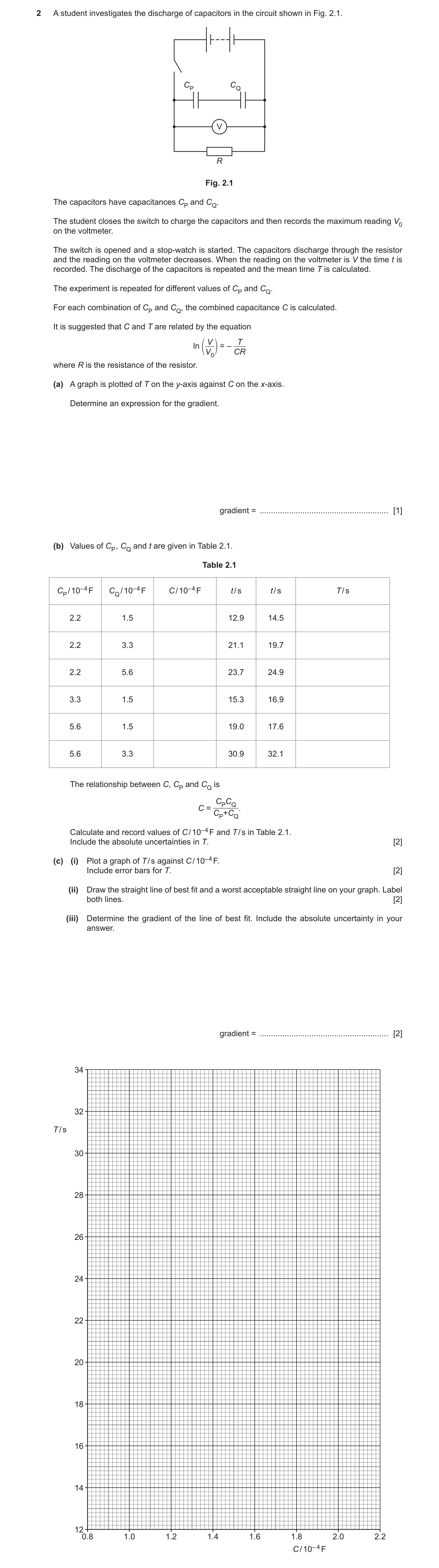
2 A student investigates the discharge of capacitors in the circuit shown in Fig. 2.1. CP CQ V R Fig. 2.1 The capacitors have capacitances CP and CQ. The student closes the switch to charge the capacitors and then records the maximum reading V0 on the voltmeter. The switch is opened and a stop‑watch is started. The capacitors discharge through the resistor and the reading on the voltmeter decreases. When the reading on the voltmeter is V the time t is recorded. The discharge of the capacitors is repeated and the mean time T is calculated. The experiment is repeated for different values of CP and CQ. For each combination of CP and CQ, the combined capacitance C is calculated. It is suggested that C and T are related by the equation V T ln = – V0 CR where R is the resistance of the resistor. (a) A graph is plotted of T on the y‑axis against C on the x‑axis. Determine an expression for the gradient. gradient = … [1] (b) Values of CP , CQ and t are given in Table 2.1. Table 2.1 CP / 10– 4 F CQ / 10– 4 F C / 10– 4 F t / s t / s T / s 2.2 1.5 12.9 14.5 2.2 3.3 21.1 19.7 2.2 5.6 23.7 24.9 3.3 1.5 15.3 16.9 5.6 1.5 19.0 17.6 5.6 3.3 30.9 32.1 The relationship between C, CP and CQ is CPCQ C = . CP+CQ Calculate and record values of C / 10– 4 F and T / s in Table 2.1. Include the absolute uncertainties in T. [2] (c) (i) Plot a graph of T / s against C / 10– 4 F. Include error bars for T. [2] (ii) Draw the straight line of best fit and a worst acceptable straight line on your graph. Label both lines. [2] (iii) Determine the gradient of the line of best fit. Include the absolute uncertainty in your answer. gradient = … [2]
9 marks
Mark scheme: 2(a) gradient = 0 ln V R V 1 2(b) C / 10–4 F T / s 0.89 or 0.892 13.7 0.8 1.3 or 1.32 20.4 0.7 1.6 or 1.58 24.3 0.6 1.0 or 1.03 16.1 0.8 1.2 or 1.18 18.3 0.7 2.1 or 2.08 31.5 0.6 Values of C and T correct as shown above. 1 Absolute uncertainties in T correct as shown above. 1 2(c)(i) Six points from (b) plotted correctly. Must be within half a small square. Diameter of points must be less than half a small square. 1 Error bars in T plotted correctly. All error bars to be plotted. Total length of bar must be accurate to less than half a small square and symmetrical. 1 Question Answer Marks 2(c)(ii) Straight line of best fit drawn. Do not accept line from top point to bottom point. Points must be balanced. Line must pass between (1.42, 22.0) and (1.45, 22.0) and between (1.95, 30.0) and (2.00, 30.0) 1 Worst acceptable line drawn (steepest or shallowest possible line that passes through all the error bars). All error bars must be plotted. 1 2(c)(iii) Gradient determined with clear substitution of data points into y / x. Distance between data points must be greater than half the length of the drawn line. 1 Gradient of worst acceptable line determined with clear substitution of data points into y / x. uncertainty = (gradient of line of best fit – gradient of worst acceptable line) or uncertainty = ½ (steepest worst line gradient – shallowest worst line gradient) 1 2(d) – 0.69 or – 0.693 and 0.06 1 2(e)(i) R determined using gradient and R given to 2 or 3 significant figures. 0 gradient ln R V V (c)(iii) (d) 1 R correctly determined using gradient and SI unit with correct power of ten for R (e.g. ). 1 Question Answer Marks 2(e)(ii) Percentage uncertainty in R with method shown. 0 0 ln gradient percentage uncertainty 100 gradient ln V V V V or Correct substitution for max/min methods. 1 Question Answer Marks 2(f) C determined to a minimum of 2 significant figures from (c)(iii) or (d) and (e)(i) with correct substitution. 60.0 gradient gradient T C or 0 60.0 ln T C V R V (e)(i) (d) 1 Absolute uncertainty in C determined with correct method used: Using gradient to determine C: gradient gradient C C Allow using R to determine C: 0 0 ln 100 ln V V C C V V (e)(ii) 1
This question in 9702/51 May/June 2023
Q10 · A student investigates the discharge of capacitors in the circuit shown in Fig 9702/53 May/June 2023
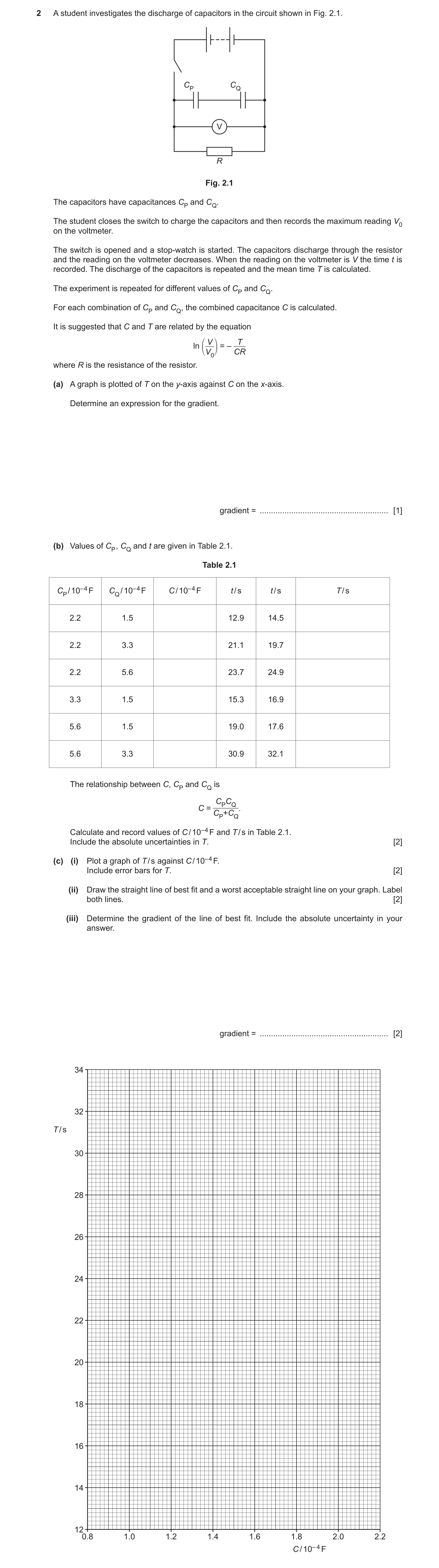
2 A student investigates the discharge of capacitors in the circuit shown in Fig. 2.1. CP CQ V R Fig. 2.1 The capacitors have capacitances CP and CQ. The student closes the switch to charge the capacitors and then records the maximum reading V0 on the voltmeter. The switch is opened and a stop‑watch is started. The capacitors discharge through the resistor and the reading on the voltmeter decreases. When the reading on the voltmeter is V the time t is recorded. The discharge of the capacitors is repeated and the mean time T is calculated. The experiment is repeated for different values of CP and CQ. For each combination of CP and CQ, the combined capacitance C is calculated. It is suggested that C and T are related by the equation V T ln = – V0 CR where R is the resistance of the resistor. (a) A graph is plotted of T on the y‑axis against C on the x‑axis. Determine an expression for the gradient. gradient = … [1] (b) Values of CP , CQ and t are given in Table 2.1. Table 2.1 CP / 10– 4 F CQ / 10– 4 F C / 10– 4 F t / s t / s T / s 2.2 1.5 12.9 14.5 2.2 3.3 21.1 19.7 2.2 5.6 23.7 24.9 3.3 1.5 15.3 16.9 5.6 1.5 19.0 17.6 5.6 3.3 30.9 32.1 The relationship between C, CP and CQ is CPCQ C = . CP+CQ Calculate and record values of C / 10– 4 F and T / s in Table 2.1. Include the absolute uncertainties in T. [2] (c) (i) Plot a graph of T / s against C / 10– 4 F. Include error bars for T. [2] (ii) Draw the straight line of best fit and a worst acceptable straight line on your graph. Label both lines. [2] (iii) Determine the gradient of the line of best fit. Include the absolute uncertainty in your answer. gradient = … [2]
9 marks
Mark scheme: 2(a) gradient = 0 ln V R V 1 2(b) C / 10–4 F T / s 0.89 or 0.892 13.7 0.8 1.3 or 1.32 20.4 0.7 1.6 or 1.58 24.3 0.6 1.0 or 1.03 16.1 0.8 1.2 or 1.18 18.3 0.7 2.1 or 2.08 31.5 0.6 Values of C and T correct as shown above. 1 Absolute uncertainties in T correct as shown above. 1 2(c)(i) Six points from (b) plotted correctly. Must be within half a small square. Diameter of points must be less than half a small square. 1 Error bars in T plotted correctly. All error bars to be plotted. Total length of bar must be accurate to less than half a small square and symmetrical. 1 Question Answer Marks 2(c)(ii) Straight line of best fit drawn. Do not accept line from top point to bottom point. Points must be balanced. Line must pass between (1.42, 22.0) and (1.45, 22.0) and between (1.95, 30.0) and (2.00, 30.0) 1 Worst acceptable line drawn (steepest or shallowest possible line that passes through all the error bars). All error bars must be plotted. 1 2(c)(iii) Gradient determined with clear substitution of data points into y / x. Distance between data points must be greater than half the length of the drawn line. 1 Gradient of worst acceptable line determined with clear substitution of data points into y / x. uncertainty = (gradient of line of best fit – gradient of worst acceptable line) or uncertainty = ½ (steepest worst line gradient – shallowest worst line gradient) 1 2(d) – 0.69 or – 0.693 and 0.06 1 2(e)(i) R determined using gradient and R given to 2 or 3 significant figures. 0 gradient ln R V V (c)(iii) (d) 1 R correctly determined using gradient and SI unit with correct power of ten for R (e.g. ). 1 Question Answer Marks 2(e)(ii) Percentage uncertainty in R with method shown. 0 0 ln gradient percentage uncertainty 100 gradient ln V V V V or Correct substitution for max/min methods. 1 Question Answer Marks 2(f) C determined to a minimum of 2 significant figures from (c)(iii) or (d) and (e)(i) with correct substitution. 60.0 gradient gradient T C or 0 60.0 ln T C V R V (e)(i) (d) 1 Absolute uncertainty in C determined with correct method used: Using gradient to determine C: gradient gradient C C Allow using R to determine C: 0 0 ln 100 ln V V C C V V (e)(ii) 1
This question in 9702/53 May/June 2023
Q11 · A student investigates the discharge of capacitors in the circuit shown in Fig 9702/52 Oct/Nov 2023
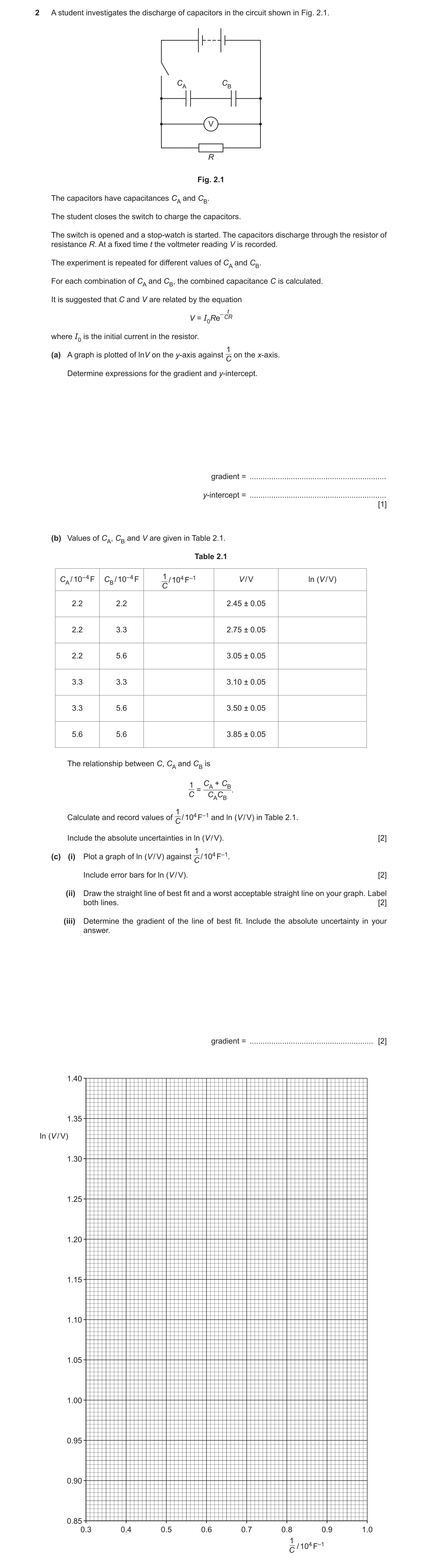
2 A student investigates the discharge of capacitors in the circuit shown in Fig. 2.1. CA CB V R Fig. 2.1 The capacitors have capacitances CA and CB. The student closes the switch to charge the capacitors. The switch is opened and a stop-watch is started. The capacitors discharge through the resistor of resistance R. At a fixed time t the voltmeter reading V is recorded. The experiment is repeated for different values of CA and CB. For each combination of CA and CB, the combined capacitance C is calculated. It is suggested that C and V are related by the equation _ t V = I0Re CR where I0 is the initial current in the resistor. 1 (a) A graph is plotted of lnV on the y-axis against on the x-axis. C Determine expressions for the gradient and y-intercept. gradient = … y-intercept = … [1] (b) Values of CA, CB and V are given in Table 2.1. Table 2.1 1 CA / 10– 4 F CB / 10– 4 F / 104 F–1 V / V ln (V / V) C 2.2 2.2 2.45 ± 0.05 2.2 3.3 2.75 ± 0.05 2.2 5.6 3.05 ± 0.05 3.3 3.3 3.10 ± 0.05 3.3 5.6 3.50 ± 0.05 5.6 5.6 3.85 ± 0.05 The relationship between C, CA and CB is 1 CA + CB = . C CACB 1 Calculate and record values of / 104 F–1 and ln (V / V) in Table 2.1. C Include the absolute uncertainties in ln (V / V). [2] 1 (c) (i) Plot a graph of ln (V / V) against / 104 F–1. C Include error bars for ln (V / V). [2] (ii) Draw the straight line of best fit and a worst acceptable straight line on your graph. Label both lines. [2] (iii) Determine the gradient of the line of best fit. Include the absolute uncertainty in your answer. gradient = … [2]
9 marks
Mark scheme: 2(a) 1 gradient = −t R y-intercept = ln I0R 2(b) 1 1 / C / 104 F–1 ln (V / V) 0.91 or 0.909 0.896 or 0.8961 0.76 or 0.758 1.012 or 1.0116 0.63 or 0.633 1.115 or 1.1151 0.61 or 0.606 1.131 or 1.1314 0.48 or 0.482 1.253 or 1.2528 0.36 or 0.357 1.348 or 1.3481 Values correct as shown above. Uncertainties in ln (V / V) from ± 0.021 or ± 0.020 to ± 0.010 or ± 0.013 1 2(c)(i) Six points from (b) plotted correctly. 1 Must be within half a small square. Diameter of points must be less than half a small square. Error bars in ln (V / V) plotted correctly. 1 All error bars to be plotted. Total length of bar must be accurate to less than half a small square and symmetrical. 2(c)(ii) Straight line of best fit drawn. 1 Do not accept line from top point to bottom point. Points must be balanced. Line must pass between (0.820, 0.95) and (0.845, 0.95) and between (0.400, 1.30) and (0.425, 1.30) Worst acceptable line drawn (steepest or shallowest possible line that passes through all the error bars). 1 All error bars must be plotted. 2(c)(iii) Gradient determined with clear substitution of data points into y / x. 1 Distance between data points must be greater than half the length of the drawn line. Gradient must be negative. Gradient determined of worst acceptable line. 1 uncertainty = (gradient of line of best fit – gradient of worst acceptable line) or uncertainty = ½ (steepest worst line gradient – shallowest worst line gradient) 2(c)(iv) y-intercept determined by substitution of correct point with consistent power of ten in m and x into y = mx + c. 1 2(d)(i) R determined using gradient. 1 30.0 30.0 R = − = gradient (c)(iii) I0 determined using y-intercept with method shown. 1 e y -intercept e (c)(iv) I0 = = R (d)(i) R and I0 determined correctly using gradient and y-intercept 1 and R and I0 given to 2 or 3 significant figures and R and I0 given with SI units with appropriate powers of ten. Units: R: or s F-1 I0: A or V F s–1 or V –1 2(d)(ii) Percentage uncertainty in R with method shown. 1 t gradient percentage uncertainty in R = + 100 t gradient or Correct substitution for max/min methods. 2(e) C determined to a minimum of 2 significant figures from (c)(iii) and (c)(iv) or (d)(i) with correct substitutions. 1 gradient gradient C = or C = − ln V − y -intercept y -intercept − ln V or t t C = − or C = R ( ln V − ln I0 R ) R ( ln I0 R − ln V )
This question in 9702/52 Oct/Nov 2023
 10
10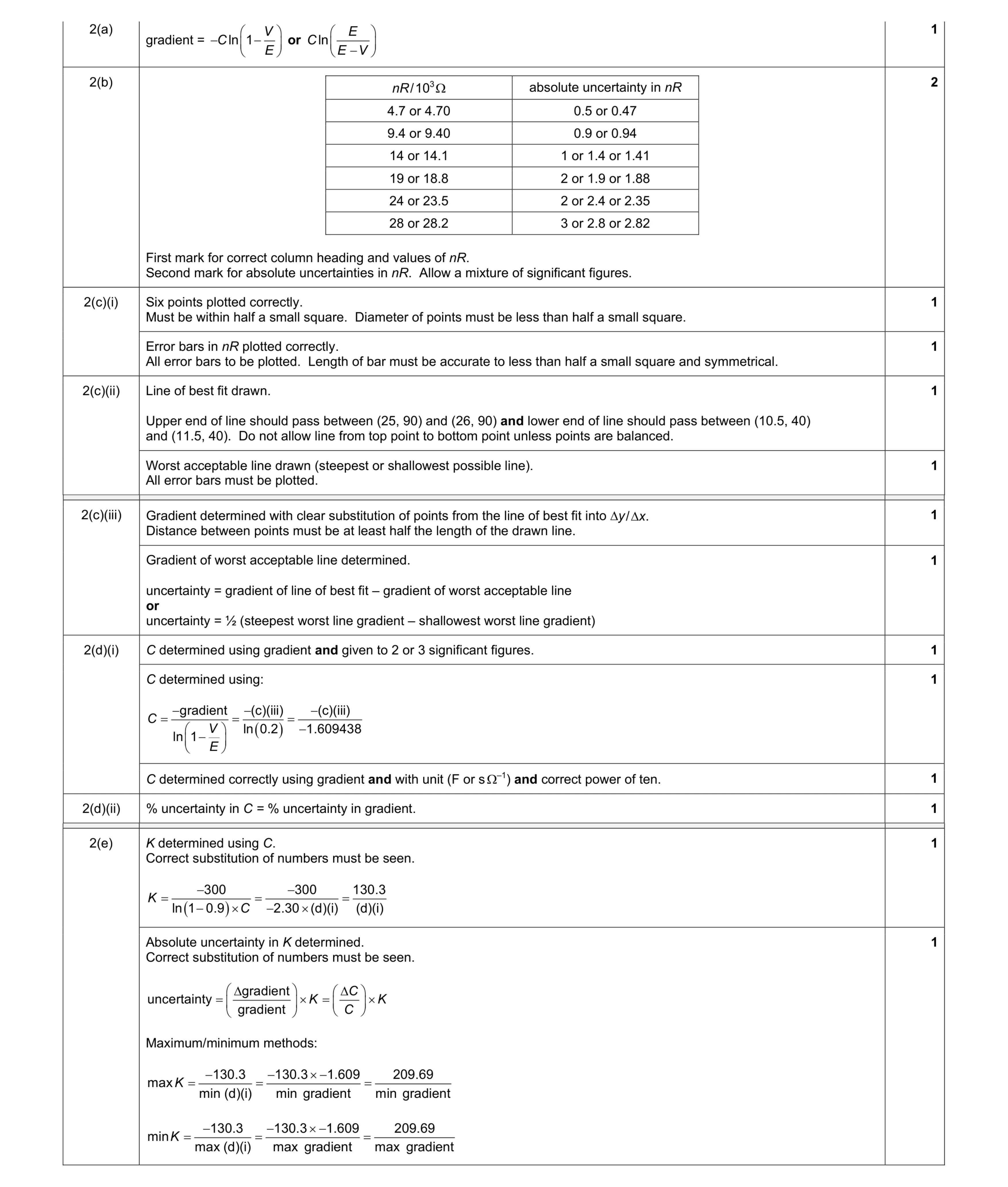 9
9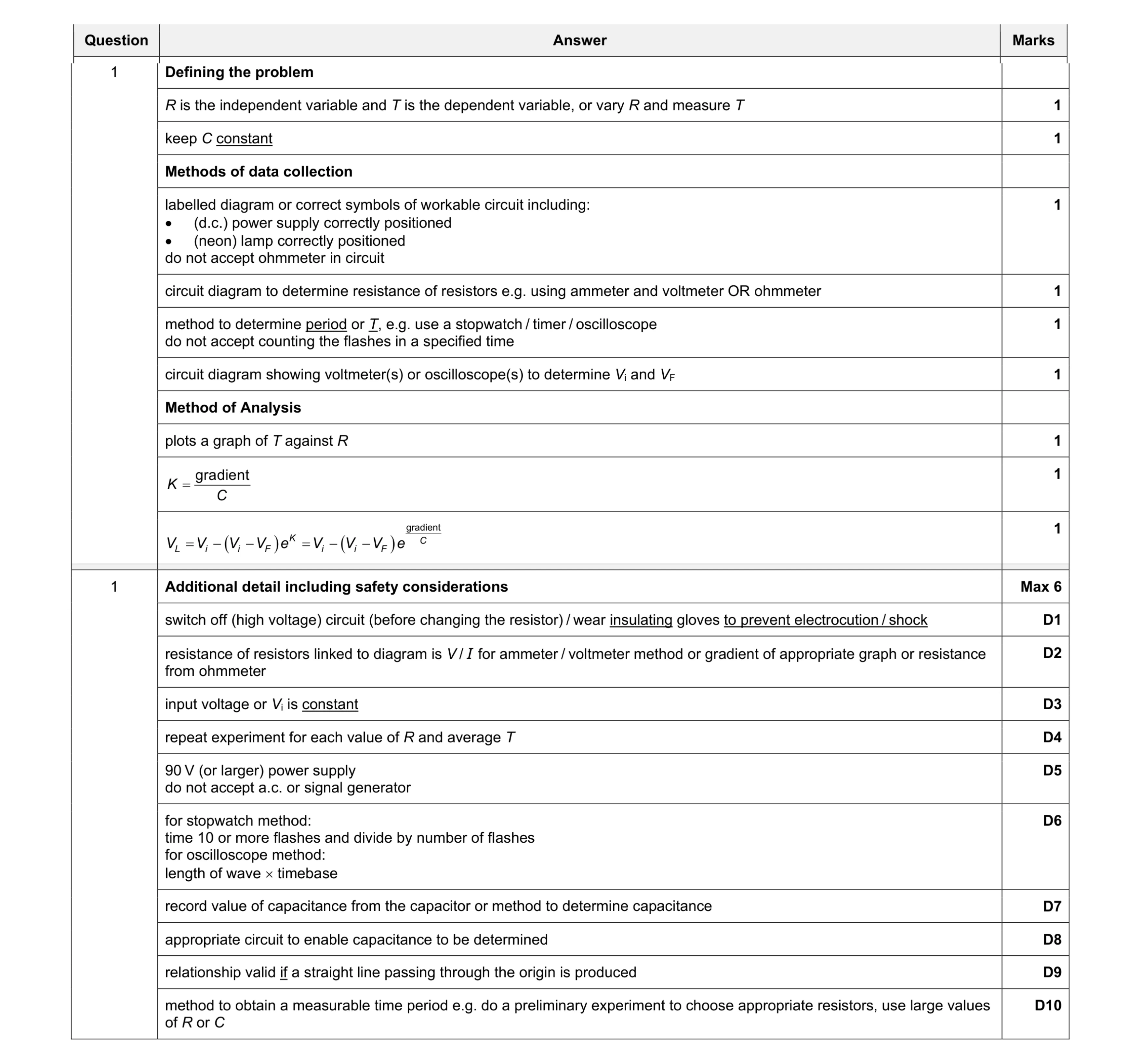 15
15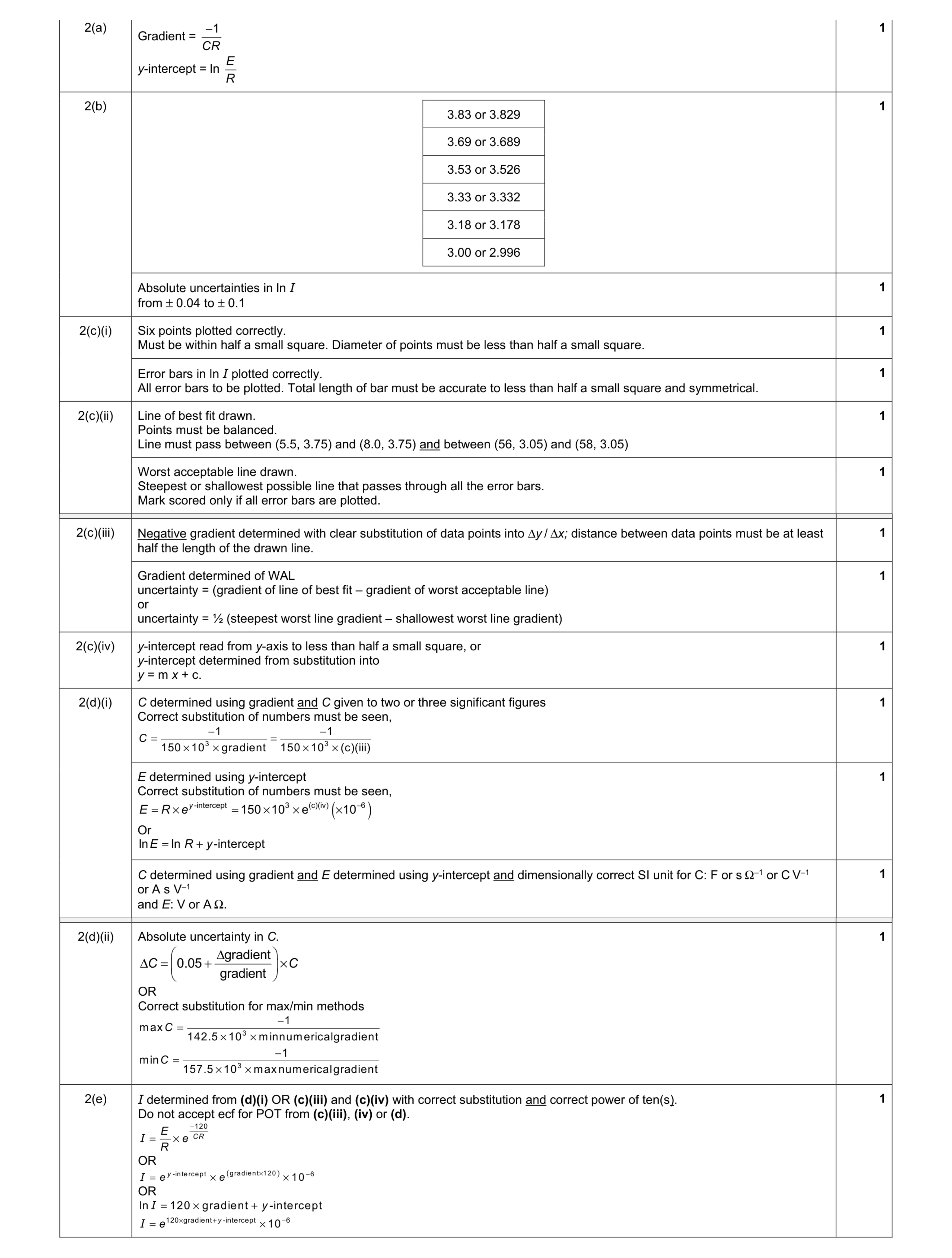 9
9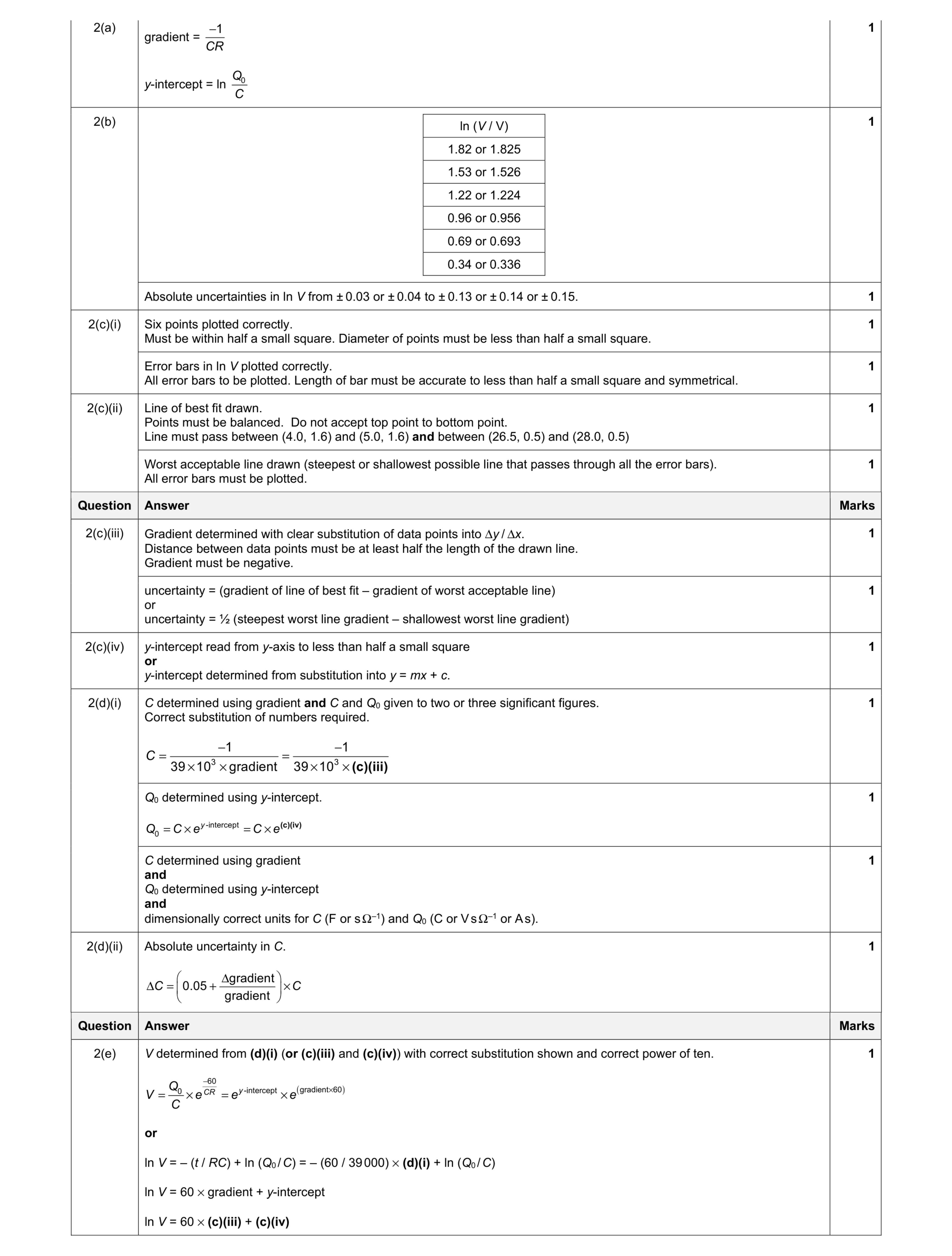 9
9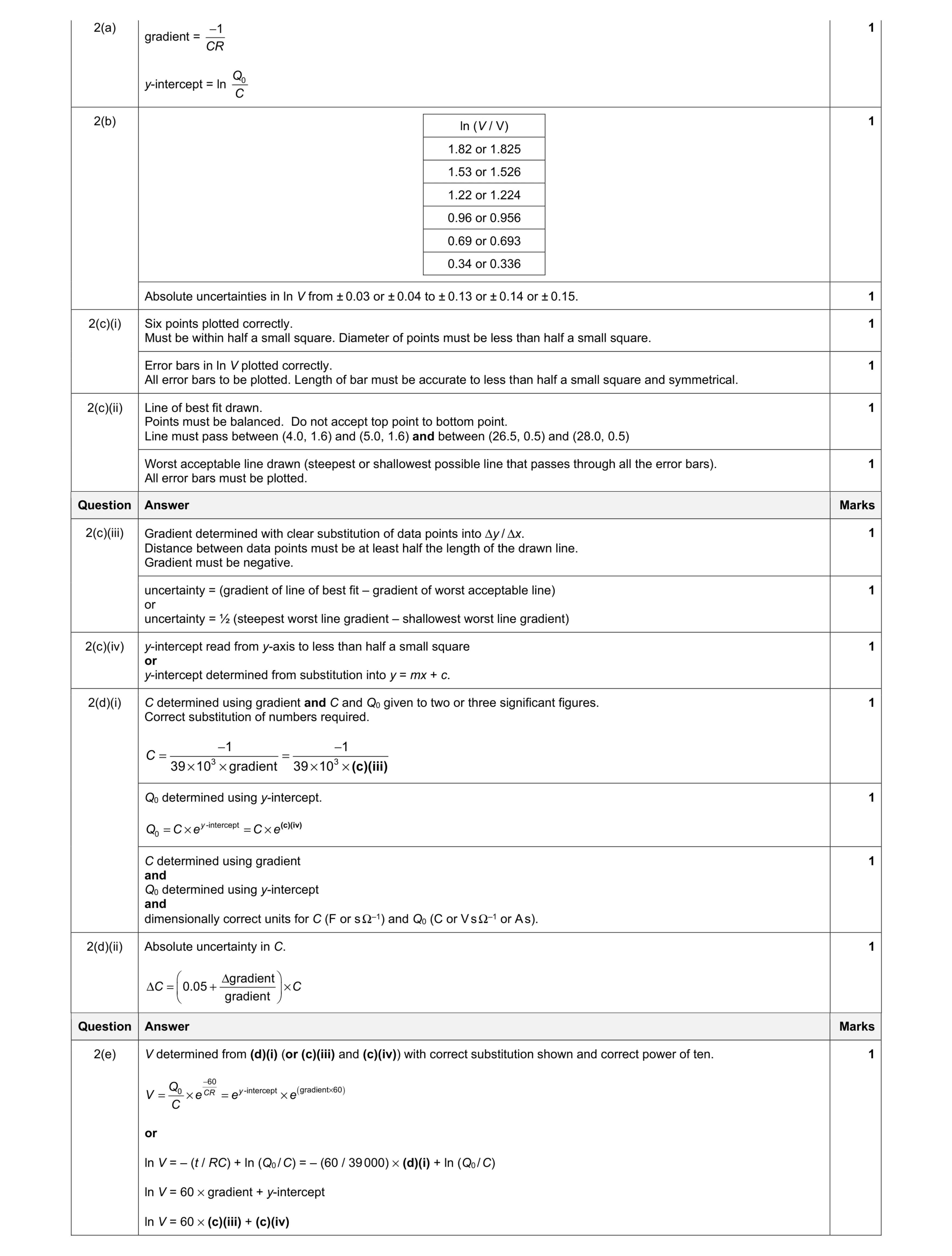 9
9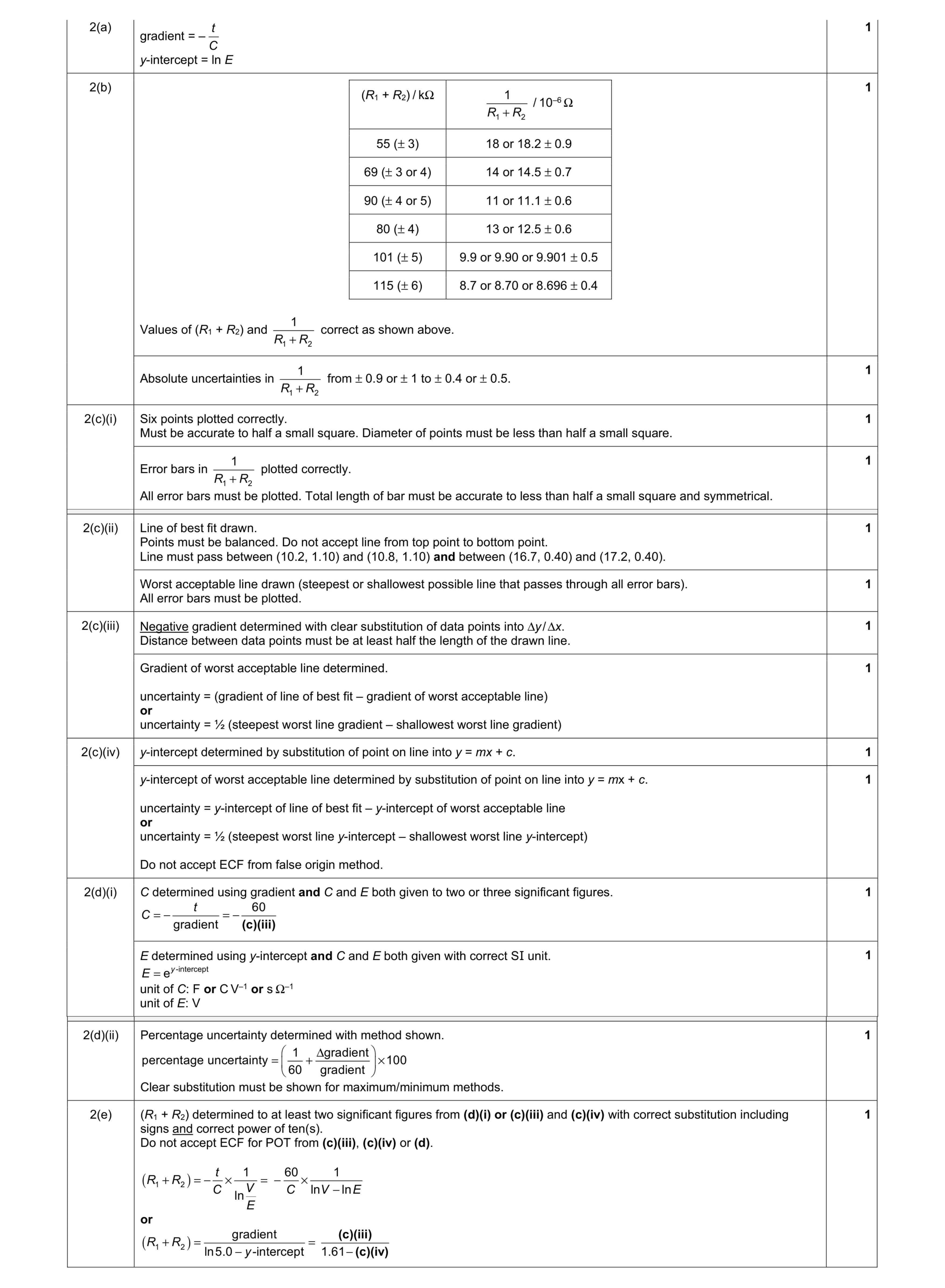 9
9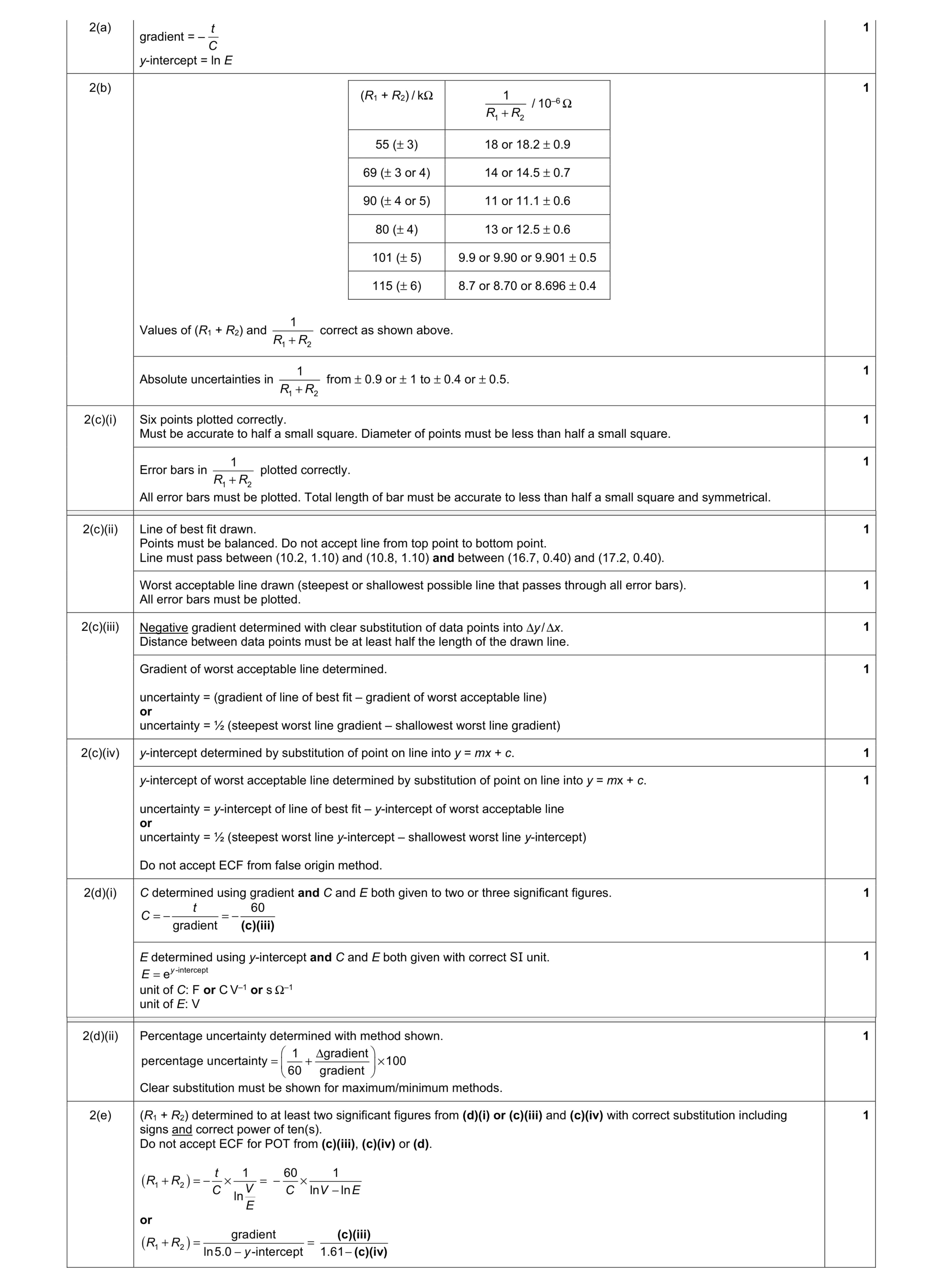 9
9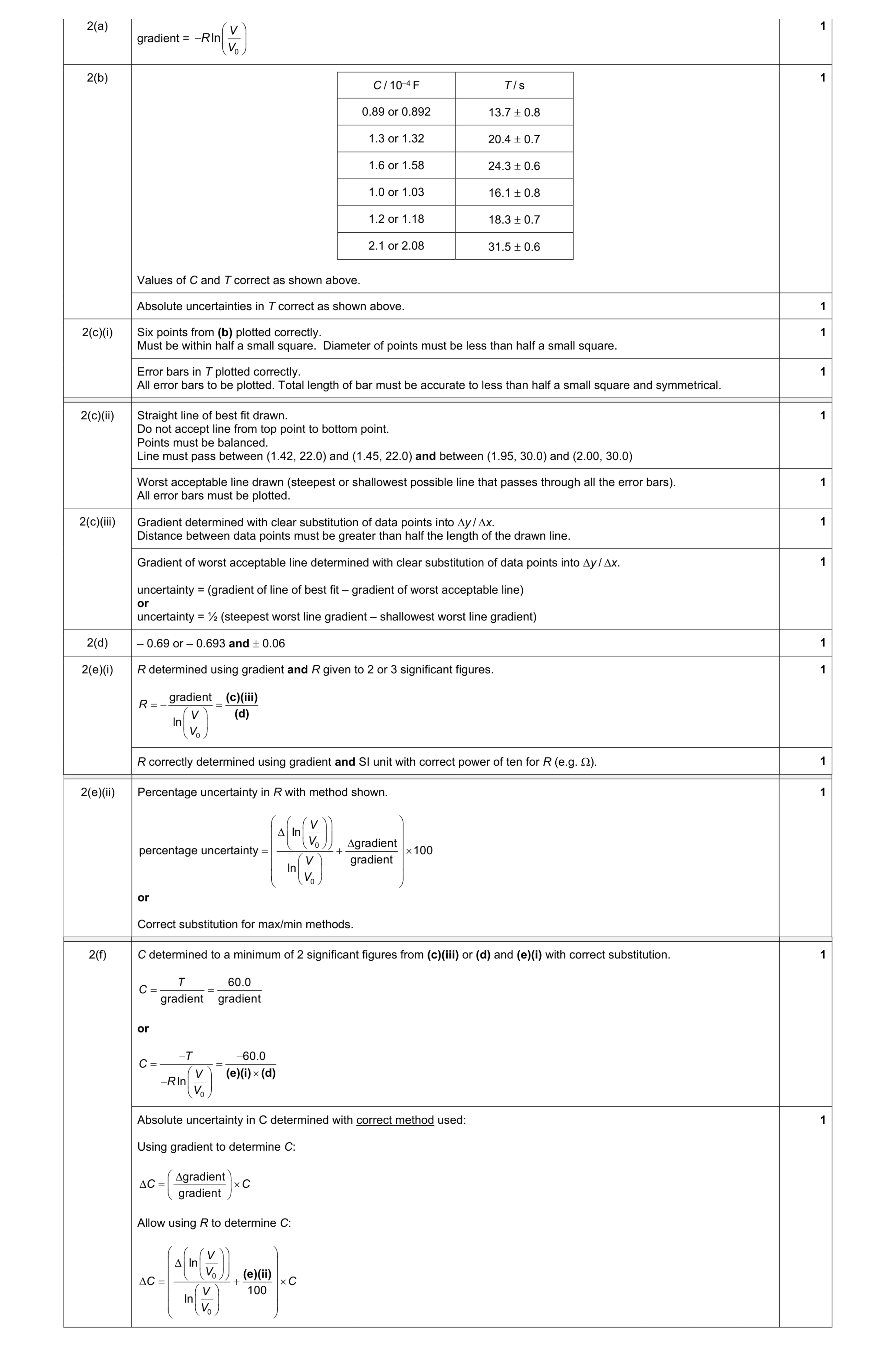 9
9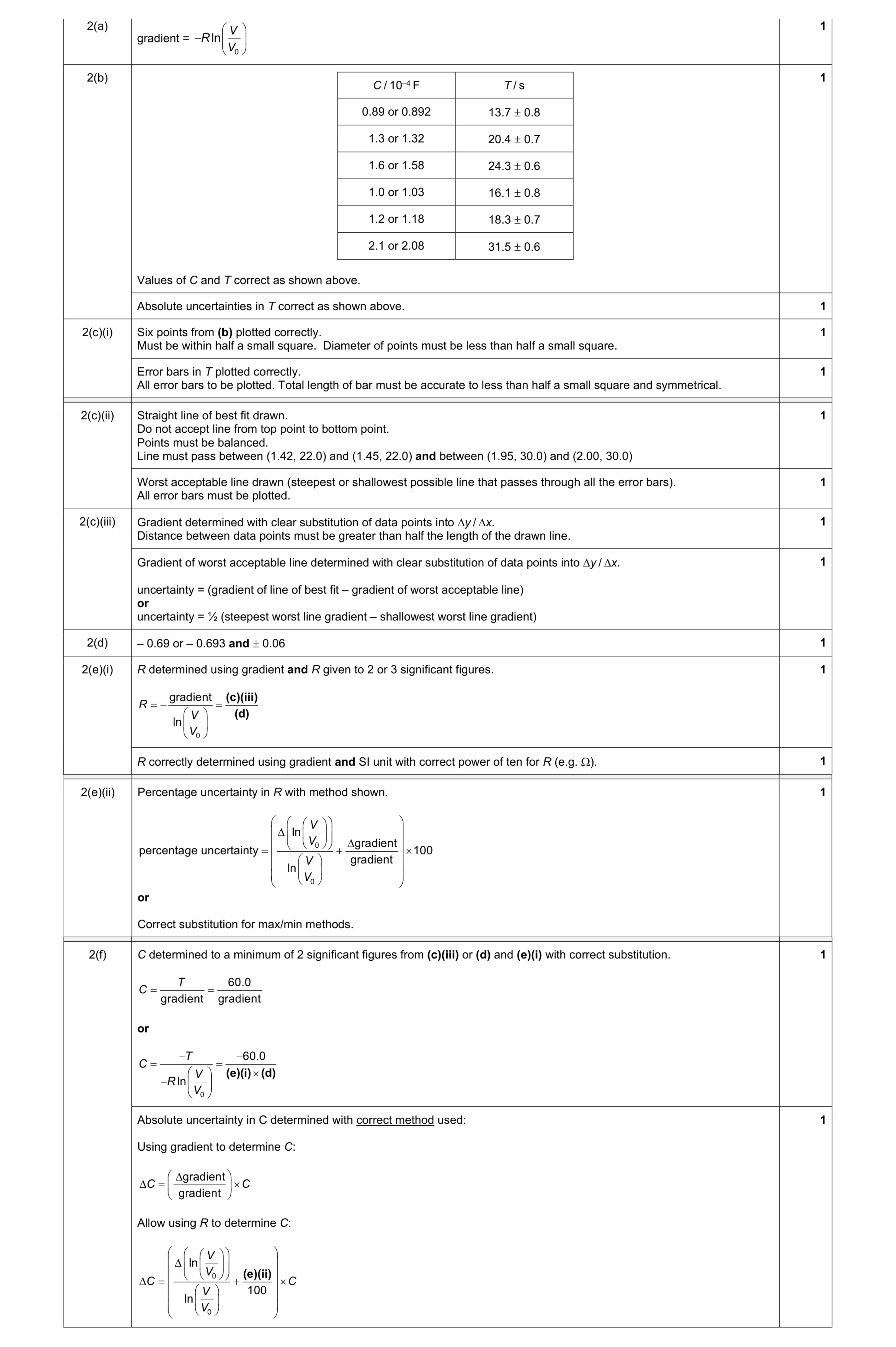 9
9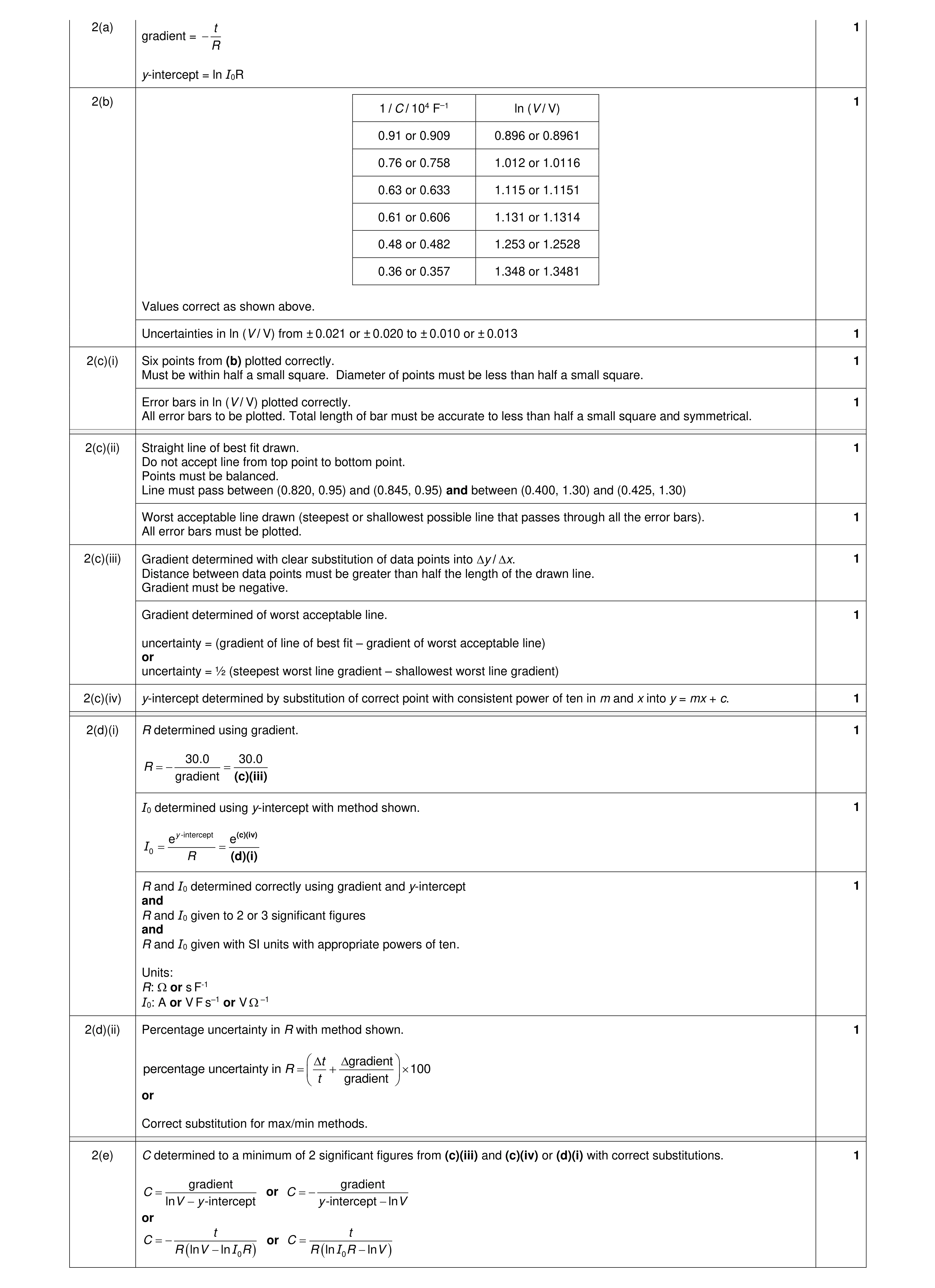 9
9