Questions as text
Q1 · A student is investigating how the period T of a simple pendulum depends on its length l… 9702/52 May/June 2010
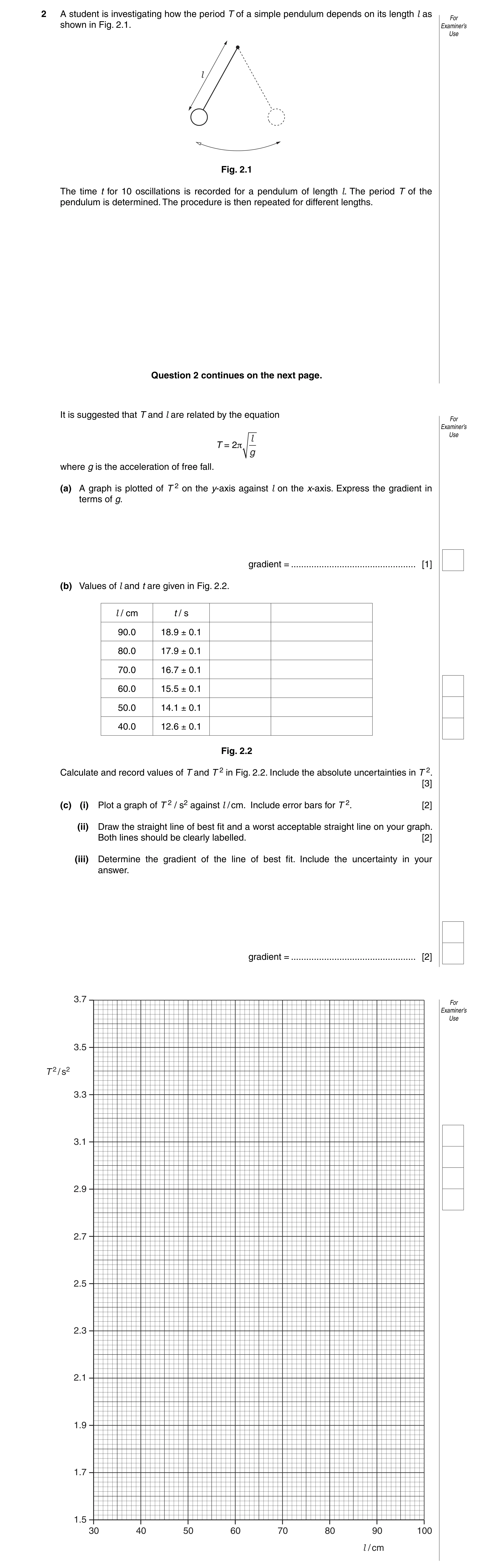
2 A student is investigating how the period T of a simple pendulum depends on its length l as For shown in Fig. 2.1. Examiner’s Use l Fig. 2.1 The time t for 10 oscillations is recorded for a pendulum of length l. The period T of the pendulum is determined. The procedure is then repeated for different lengths. Question 2 continues on the next page. It is suggested that T and l are related by the equation For Examiner’s l Use T = 2π g where g is the acceleration of free fall. (a) A graph is plotted of T 2 on the y-axis against l on the x-axis. Express the gradient in terms of g. gradient = … [1] (b) Values of l and t are given in Fig. 2.2. l / cm t / s 90.0 18.9 ± 0.1 80.0 17.9 ± 0.1 70.0 16.7 ± 0.1 60.0 15.5 ± 0.1 50.0 14.1 ± 0.1 40.0 12.6 ± 0.1 Fig. 2.2 Calculate and record values of T and T 2 in Fig. 2.2. Include the absolute uncertainties in T 2. [3] (c) (i) Plot a graph of T 2 / s2 against l / cm. Include error bars for T 2. [2] (ii) Draw the straight line of best fit and a worst acceptable straight line on your graph. Both lines should be clearly labelled. [2] (iii) Determine the gradient of the line of best fit. Include the uncertainty in your answer. gradient = … [2] 3.7 For Examiner’s Use 3.5 T 2 / s2 3.3 3.1 2.9 2.7 2.5 2.3 2.1 1.9 1.7 1.5 30 40 50 60 70 80 90 100 l / cm
10 marks
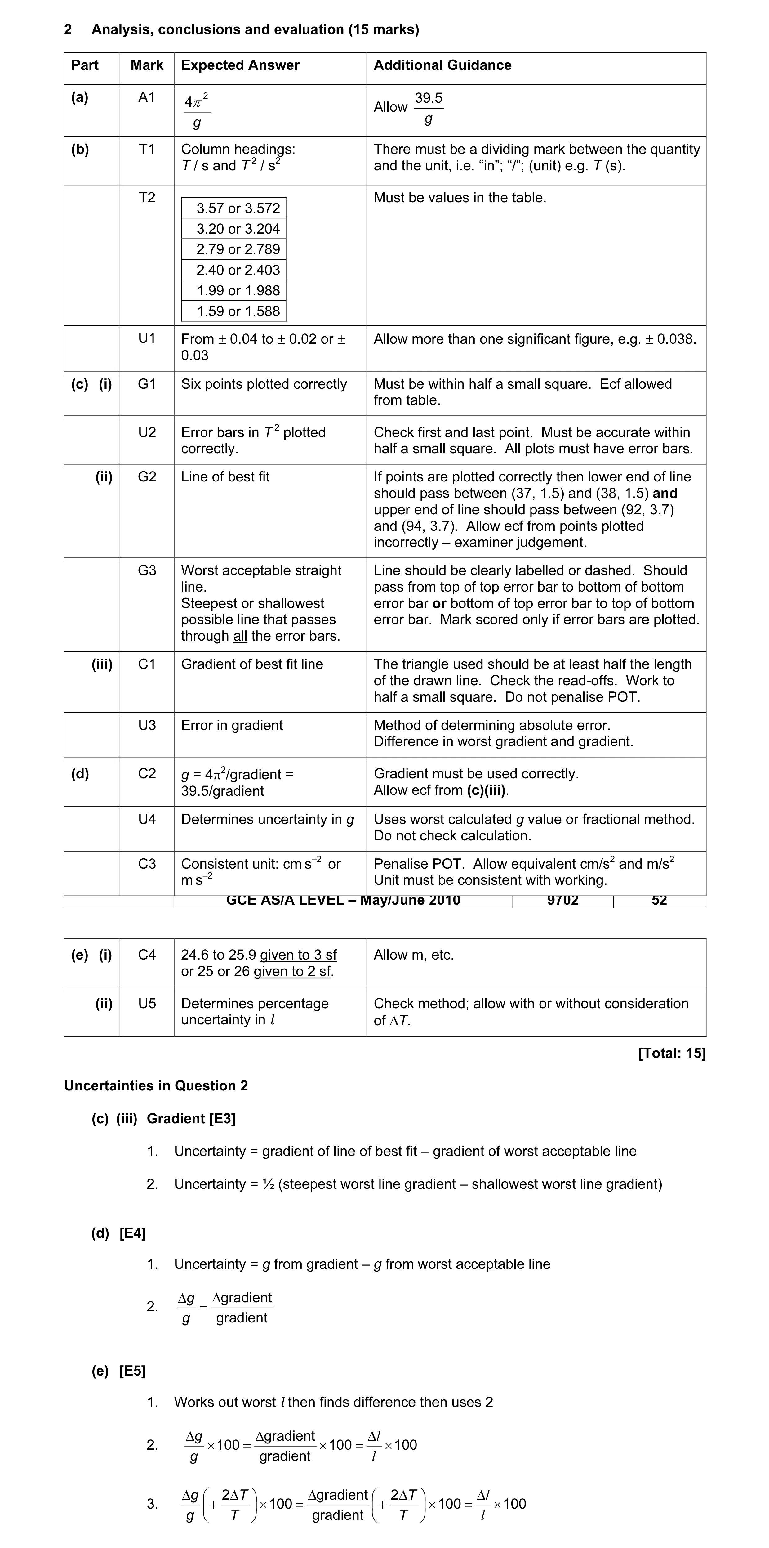
Mark scheme: 2 Analysis, conclusions and evaluation (15 marks) Part Mark Expected Answer Additional Guidance (a) A1 2 39.5 4π Allow g g (b) T1 Column headings: There must be a dividing mark between the quantity T / s and T 2 / s2 and the unit, i.e. “in”; “/”; (unit) e.g. T (s). T2 Must be values in the table. 3.57 or 3.572 3.20 or 3.204 2.79 or 2.789 2.40 or 2.403 1.99 or 1.988 1.59 or 1.588 U1 From ± 0.04 to ± 0.02 or ± Allow more than one significant figure, e.g. ± 0.038. 0.03 (c) (i) G1 Six points plotted correctly Must be within half a small square. Ecf allowed from table. U2 Error bars in T 2 plotted Check first and last point. Must be accurate within correctly. half a small square. All plots must have error bars. (ii) G2 Line of best fit If points are plotted correctly then lower end of line should pass between (37, 1.5) and (38, 1.5) and upper end of line should pass between (92, 3.7) and (94, 3.7). Allow ecf from points plotted incorrectly – examiner judgement. G3 Worst acceptable straight Line should be clearly labelled or dashed. Should line. pass from top of top error bar to bottom of bottom Steepest or shallowest error bar or bottom of top error bar to top of bottom possible line that passes error bar. Mark scored only if error bars are plotted. through all the error bars. (iii) C1 Gradient of best fit line The triangle used should be at least half the length of the drawn line. Check the read-offs. Work to half a small square. Do not penalise POT. U3 Error in gradient Method of determining absolute error. Difference in worst gradient and gradient. (d) C2 g = 4π2/gradient = Gradient must be used correctly. 39.5/gradient Allow ecf from (c)(iii). U4 Determines uncertainty in g Uses worst calculated g value or fractional method. Do not check calculation. C3 Consistent unit: cm s–2 or Penalise POT. Allow equivalent cm/s2 and m/s2 m s–2 Unit must be consistent with working. GCE AS/A LEVEL – May/June 2010 9702 52 (e) (i) C4 24.6 to 25.9 given to 3 sf Allow m, etc. or 25 or 26 given to 2 sf. (ii) U5 Determines percentage Check method; allow with or without consideration uncertainty in l of ∆T. [Total: 15] Uncertainties in Question 2 (c) (iii) Gradient [E3] 1. Uncertainty = gradient of line of best fit – gradient of worst acceptable line 2. Uncertainty = ½ (steepest worst line gradient – shallowest worst line gradient) (d) [E4] 1. Uncertainty = g from gradient – g from worst acceptable line ∆g ∆gradient 2. = g gradient (e) [E5] 1. Works out worst l then finds difference then uses 2 ∆g ∆gradient ∆l 2. × 100 = × 100 = × 100 g gradient l ∆g 2 ∆T ∆gradient 2 ∆T ∆l 3. + × 100 = + × 100 = × 100 g T gradient T l
This question in 9702/52 May/June 2010
Q2 · A student is investigating how the period T of a simple pendulum depends on its length l… 9702/53 May/June 2010
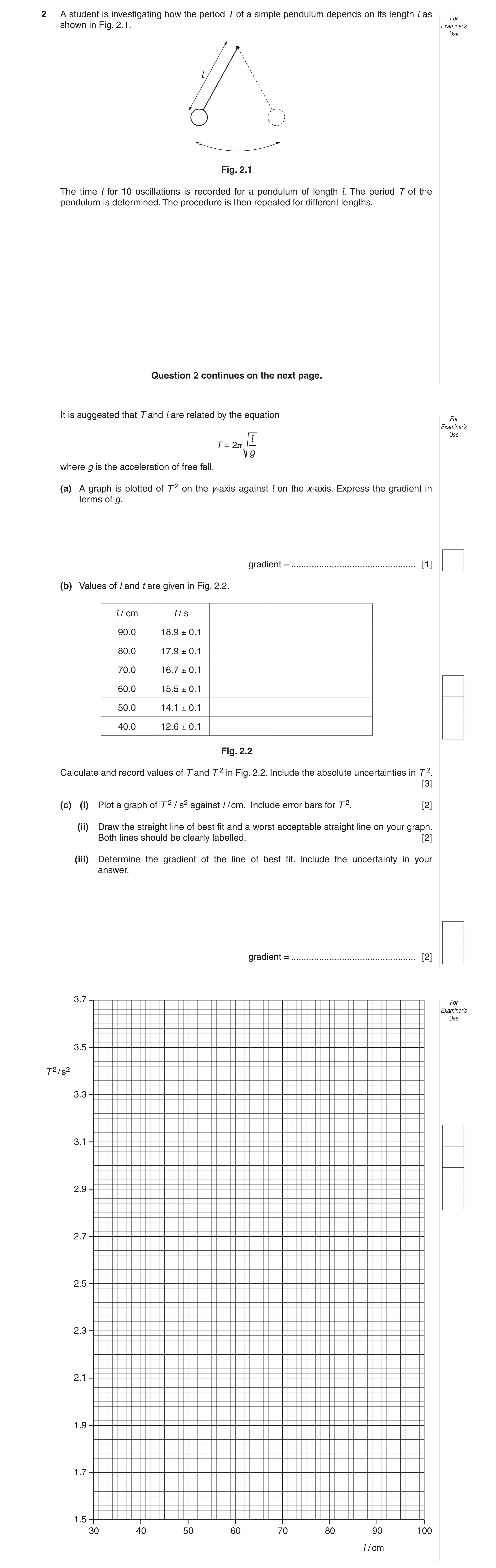
2 A student is investigating how the period T of a simple pendulum depends on its length l as For shown in Fig. 2.1. Examiner’s Use l Fig. 2.1 The time t for 10 oscillations is recorded for a pendulum of length l. The period T of the pendulum is determined. The procedure is then repeated for different lengths. Question 2 continues on the next page. It is suggested that T and l are related by the equation For Examiner’s l Use T = 2π g where g is the acceleration of free fall. (a) A graph is plotted of T 2 on the y-axis against l on the x-axis. Express the gradient in terms of g. gradient = … [1] (b) Values of l and t are given in Fig. 2.2. l / cm t / s 90.0 18.9 ± 0.1 80.0 17.9 ± 0.1 70.0 16.7 ± 0.1 60.0 15.5 ± 0.1 50.0 14.1 ± 0.1 40.0 12.6 ± 0.1 Fig. 2.2 Calculate and record values of T and T 2 in Fig. 2.2. Include the absolute uncertainties in T 2. [3] (c) (i) Plot a graph of T 2 / s2 against l / cm. Include error bars for T 2. [2] (ii) Draw the straight line of best fit and a worst acceptable straight line on your graph. Both lines should be clearly labelled. [2] (iii) Determine the gradient of the line of best fit. Include the uncertainty in your answer. gradient = … [2] 3.7 For Examiner’s Use 3.5 T 2 / s2 3.3 3.1 2.9 2.7 2.5 2.3 2.1 1.9 1.7 1.5 30 40 50 60 70 80 90 100 l / cm
10 marks
Mark scheme: 2 Analysis, conclusions and evaluation (15 marks) Part Mark Expected Answer Additional Guidance (a) A1 2 39.5 4π Allow g g (b) T1 Column headings: There must be a dividing mark between the quantity T / s and T 2 / s2 and the unit, i.e. “in”; “/”; (unit) e.g. T (s). T2 Must be values in the table. 3.57 or 3.572 3.20 or 3.204 2.79 or 2.789 2.40 or 2.403 1.99 or 1.988 1.59 or 1.588 U1 From ± 0.04 to ± 0.02 or ± Allow more than one significant figure, e.g. ± 0.038. 0.03 (c) (i) G1 Six points plotted correctly Must be within half a small square. Ecf allowed from table. U2 Error bars in T 2 plotted Check first and last point. Must be accurate within correctly. half a small square. All plots must have error bars. (ii) G2 Line of best fit If points are plotted correctly then lower end of line should pass between (37, 1.5) and (38, 1.5) and upper end of line should pass between (92, 3.7) and (94, 3.7). Allow ecf from points plotted incorrectly – examiner judgement. G3 Worst acceptable straight Line should be clearly labelled or dashed. Should line. pass from top of top error bar to bottom of bottom Steepest or shallowest error bar or bottom of top error bar to top of bottom possible line that passes error bar. Mark scored only if error bars are plotted. through all the error bars. (iii) C1 Gradient of best fit line The triangle used should be at least half the length of the drawn line. Check the read-offs. Work to half a small square. Do not penalise POT. U3 Error in gradient Method of determining absolute error. Difference in worst gradient and gradient. (d) C2 g = 4π2/gradient = Gradient must be used correctly. 39.5/gradient Allow ecf from (c)(iii). U4 Determines uncertainty in g Uses worst calculated g value or fractional method. Do not check calculation. C3 Consistent unit: cm s–2 or Penalise POT. Allow equivalent cm/s2 and m/s2 m s–2 Unit must be consistent with working. GCE AS/A LEVEL – May/June 2010 9702 53 (e) (i) C4 24.6 to 25.9 given to 3 sf Allow m, etc. or 25 or 26 given to 2 sf. (ii) U5 Determines percentage Check method; allow with or without consideration uncertainty in l of ∆T. [Total: 15] Uncertainties in Question 2 (c) (iii) Gradient [E3] 1. Uncertainty = gradient of line of best fit – gradient of worst acceptable line 2. Uncertainty = ½ (steepest worst line gradient – shallowest worst line gradient) (d) [E4] 1. Uncertainty = g from gradient – g from worst acceptable line ∆g ∆gradient 2. = g gradient (e) [E5] 1. Works out worst l then finds difference then uses 2 ∆g ∆gradient ∆l 2. × 100 = × 100 = × 100 g gradient l ∆g 2 ∆T ∆gradient 2 ∆T ∆l 3. + × 100 = + × 100 = × 100 g T gradient T l
This question in 9702/53 May/June 2010
Q3 · A student is investigating how the period T of a simple pendulum depends on its For… 9702/51 Oct/Nov 2010
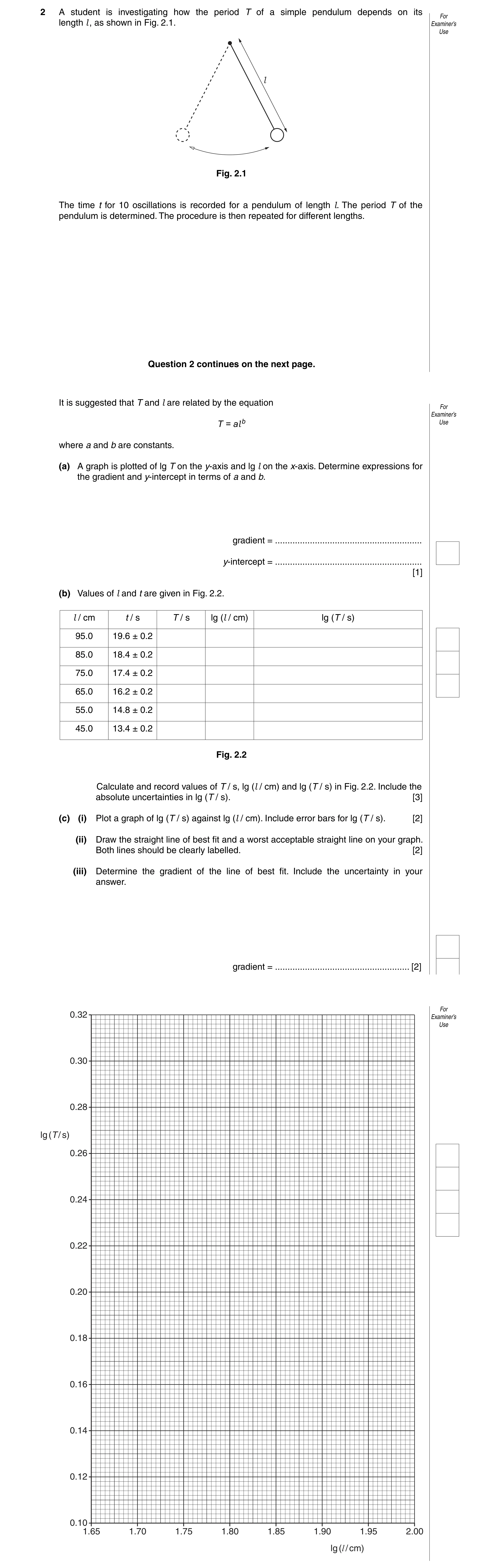
2 A student is investigating how the period T of a simple pendulum depends on its For length l , as shown in Fig. 2.1. Examiner’s Use l Fig. 2.1 The time t for 10 oscillations is recorded for a pendulum of length l. The period T of the pendulum is determined. The procedure is then repeated for different lengths. Question 2 continues on the next page. It is suggested that T and l are related by the equation For Examiner’s T = al b Use where a and b are constants. (a) A graph is plotted of lg T on the y-axis and lg l on the x-axis. Determine expressions for the gradient and y-intercept in terms of a and b. gradient = … y-intercept = … [1] (b) Values of l and t are given in Fig. 2.2. l / cm t / s T / s lg (l / cm) lg (T / s) 95.0 19.6 ± 0.2 85.0 18.4 ± 0.2 75.0 17.4 ± 0.2 65.0 16.2 ± 0.2 55.0 14.8 ± 0.2 45.0 13.4 ± 0.2 Fig. 2.2 Calculate and record values of T / s, lg (l / cm) and lg (T / s) in Fig. 2.2. Include the absolute uncertainties in lg (T / s). [3] (c) (i) Plot a graph of lg (T / s) against lg (l / cm). Include error bars for lg (T / s). [2] (ii) Draw the straight line of best fit and a worst acceptable straight line on your graph. Both lines should be clearly labelled. [2] (iii) Determine the gradient of the line of best fit. Include the uncertainty in your answer. gradient = … [2] For 0.32 Examiner’s Use 0.30 0.28 lg (T / s) 0.26 0.24 0.22 0.20 0.18 0.16 0.14 0.12 0.10 1.65 1.70 1.75 1.80 1.85 1.90 1.95 2.00 lg (l / cm)
10 marks
Mark scheme: 2 Analysis, conclusions and evaluation (15 marks) Part Mark Expected Answer Additional Guidance (a) A1 Gradient = b Allow log a but not ln a y-intercept = lg a (b) T1 T1 for lg l column – ignore rounding errors; min T2 1.9777 0.292 or 0.2923 2 dp. 1.9294 0.265 or 0.2648 T2 for lg T column – must be values given A mixture is allowed 1.8751 0.241 or 0.2405 1.8129 0.210 or 0.2095 1.7404 0.170 or 0.1703 1.6532 0.127 or 0.1271 U1 From ± 0.004 or ± 0.005 to ± 0.006 Allow more than one significant figure. or ± 0.007 (c) (i) G1 Six points plotted correctly Must be within half a small square; penalise ≥ half a small square. Penalise ‘blobs’ ≥ half a small square. Ecf allowed from table. U2 Error bars in lg (T/s) plotted All error bars must be plotted. Check first and correctly. last point. Must be accurate within half a small square; penalise ≥ half a small square. (ii) G2 Line of best fit If points are plotted correctly then lower end of line should pass between (1.65, 0.124) and (1.65, 0.128) and upper end of line should pass between (2.00, 0.300) and (2.00, 0.306). Allow ecf from points plotted incorrectly; five trend plots needed – examiner judgement. G3 Worst acceptable straight line. Line should be clearly labelled or dashed. Steepest or shallowest possible Should pass from top of top error bar to bottom line that passes through all the of bottom error bar or bottom of top error bar to error bars. top of bottom error bar. Mark scored only if all error bars are plotted. (iii) C1 Gradient of best fit line The triangle used should be at least half the length of the drawn line. Check the read offs. Work to half a small square; penalise ≥ half a small square. U3 Uncertainty in gradient Method of determining absolute uncertainty Difference in worst gradient and gradient. (iv) C2 y-intercept Must be negative. Check substitution of point from line into c = y – mx. Allow ecf from (c)(iii). GCE A/AS LEVEL – October/November 2010 9702 51 U4 Uncertainty in y-intercept Method of determining absolute uncertainty Difference in worst y-intercept and y-intercept. Do not allow ecf from false origin read-off (FOX). Allow ecf from (c)(iv). (d) C3 a = 10y-intercept y-intercept must be used. Expect an answer of about 0.19. If FOX expect answer of about 1.3. C4 b = gradient and in the range 0.495 Allow 0.50 to 0.52 to 2 sf to 0.520 and to 2 or 3 sf Penalise 1 sf or ≥4 sf U5 Absolute uncertainty in a and b Difference in a and worst a. Uncertainty in b should be the same as the uncertainty in the gradient. [Total: 15] Uncertainties in Question 2 (c) (iii) Gradient [U3] 1. Uncertainty = gradient of line of best fit – gradient of worst acceptable line 2. Uncertainty = ½ (steepest worst line gradient – shallowest worst line gradient) (c) (iv) [U4] 1. Uncertainty = y-intercept of line of best fit – y-intercept of worst acceptable line 2. Uncertainty = ½ (y-intercept of steepest worst line – y-intercept of shallowest worst line) (d) [U5] 1. Uncertainty = 10 best y-intercept - 10 worst y-intercept
This question in 9702/51 Oct/Nov 2010
Q4 · A student is investigating how the period T of a simple pendulum depends on its For… 9702/52 Oct/Nov 2010
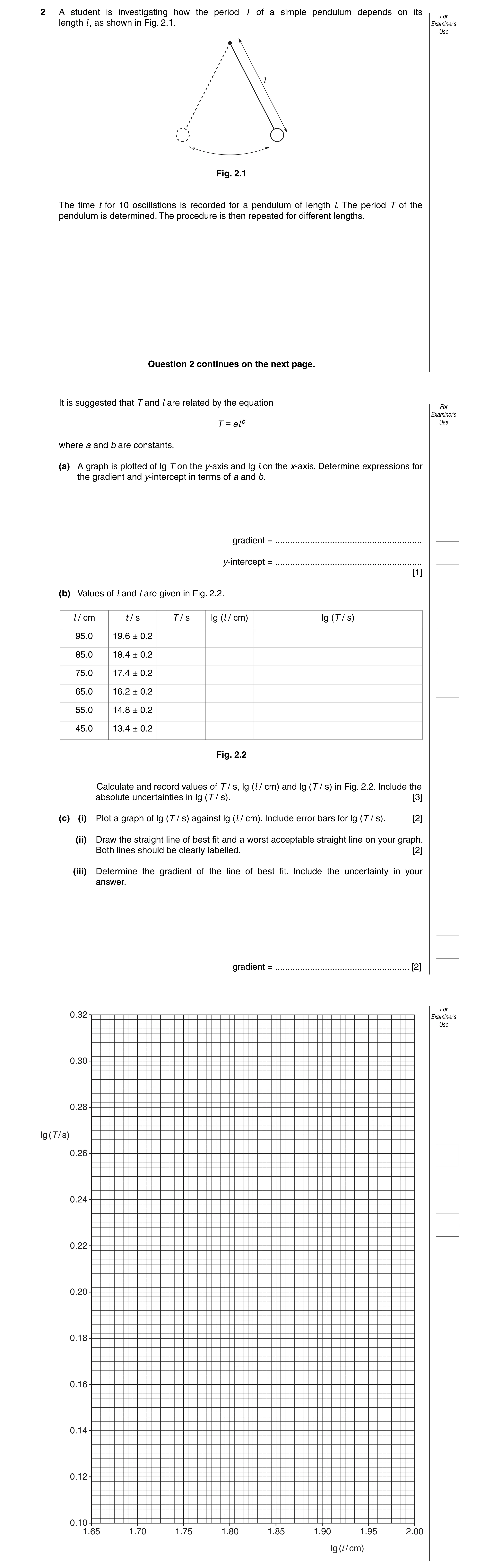
2 A student is investigating how the period T of a simple pendulum depends on its For length l , as shown in Fig. 2.1. Examiner’s Use l Fig. 2.1 The time t for 10 oscillations is recorded for a pendulum of length l. The period T of the pendulum is determined. The procedure is then repeated for different lengths. Question 2 continues on the next page. It is suggested that T and l are related by the equation For Examiner’s T = al b Use where a and b are constants. (a) A graph is plotted of lg T on the y-axis and lg l on the x-axis. Determine expressions for the gradient and y-intercept in terms of a and b. gradient = … y-intercept = … [1] (b) Values of l and t are given in Fig. 2.2. l / cm t / s T / s lg (l / cm) lg (T / s) 95.0 19.6 ± 0.2 85.0 18.4 ± 0.2 75.0 17.4 ± 0.2 65.0 16.2 ± 0.2 55.0 14.8 ± 0.2 45.0 13.4 ± 0.2 Fig. 2.2 Calculate and record values of T / s, lg (l / cm) and lg (T / s) in Fig. 2.2. Include the absolute uncertainties in lg (T / s). [3] (c) (i) Plot a graph of lg (T / s) against lg (l / cm). Include error bars for lg (T / s). [2] (ii) Draw the straight line of best fit and a worst acceptable straight line on your graph. Both lines should be clearly labelled. [2] (iii) Determine the gradient of the line of best fit. Include the uncertainty in your answer. gradient = … [2] For 0.32 Examiner’s Use 0.30 0.28 lg (T / s) 0.26 0.24 0.22 0.20 0.18 0.16 0.14 0.12 0.10 1.65 1.70 1.75 1.80 1.85 1.90 1.95 2.00 lg (l / cm)
10 marks
Mark scheme: 2 Analysis, conclusions and evaluation (15 marks) Part Mark Expected Answer Additional Guidance (a) A1 Gradient = b Allow log a but not ln a y-intercept = lg a (b) T1 T1 for lg l column – ignore rounding errors; min T2 1.9777 0.292 or 0.2923 2 dp. 1.9294 0.265 or 0.2648 T2 for lg T column – must be values given A mixture is allowed 1.8751 0.241 or 0.2405 1.8129 0.210 or 0.2095 1.7404 0.170 or 0.1703 1.6532 0.127 or 0.1271 U1 From ± 0.004 or ± 0.005 to ± 0.006 Allow more than one significant figure. or ± 0.007 (c) (i) G1 Six points plotted correctly Must be within half a small square; penalise ≥ half a small square. Penalise ‘blobs’ ≥ half a small square. Ecf allowed from table. U2 Error bars in lg (T/s) plotted All error bars must be plotted. Check first and correctly. last point. Must be accurate within half a small square; penalise ≥ half a small square. (ii) G2 Line of best fit If points are plotted correctly then lower end of line should pass between (1.65, 0.124) and (1.65, 0.128) and upper end of line should pass between (2.00, 0.300) and (2.00, 0.306). Allow ecf from points plotted incorrectly; five trend plots needed – examiner judgement. G3 Worst acceptable straight line. Line should be clearly labelled or dashed. Steepest or shallowest possible Should pass from top of top error bar to bottom line that passes through all the of bottom error bar or bottom of top error bar to error bars. top of bottom error bar. Mark scored only if all error bars are plotted. (iii) C1 Gradient of best fit line The triangle used should be at least half the length of the drawn line. Check the read offs. Work to half a small square; penalise ≥ half a small square. U3 Uncertainty in gradient Method of determining absolute uncertainty Difference in worst gradient and gradient. (iv) C2 y-intercept Must be negative. Check substitution of point from line into c = y – mx. Allow ecf from (c)(iii). GCE A/AS LEVEL – October/November 2010 9702 52 U4 Uncertainty in y-intercept Method of determining absolute uncertainty Difference in worst y-intercept and y-intercept. Do not allow ecf from false origin read-off (FOX). Allow ecf from (c)(iv). (d) C3 a = 10y-intercept y-intercept must be used. Expect an answer of about 0.19. If FOX expect answer of about 1.3. C4 b = gradient and in the range 0.495 Allow 0.50 to 0.52 to 2 sf to 0.520 and to 2 or 3 sf Penalise 1 sf or ≥4 sf U5 Absolute uncertainty in a and b Difference in a and worst a. Uncertainty in b should be the same as the uncertainty in the gradient. [Total: 15] Uncertainties in Question 2 (c) (iii) Gradient [U3] 1. Uncertainty = gradient of line of best fit – gradient of worst acceptable line 2. Uncertainty = ½ (steepest worst line gradient – shallowest worst line gradient) (c) (iv) [U4] 1. Uncertainty = y-intercept of line of best fit – y-intercept of worst acceptable line 2. Uncertainty = ½ (y-intercept of steepest worst line – y-intercept of shallowest worst line) (d) [U5] 1. Uncertainty = 10 best y-intercept - 10 worst y-intercept
This question in 9702/52 Oct/Nov 2010
Q5 · A trolley is attached to springs, as shown in Fig 2.1 9702/53 Oct/Nov 2012
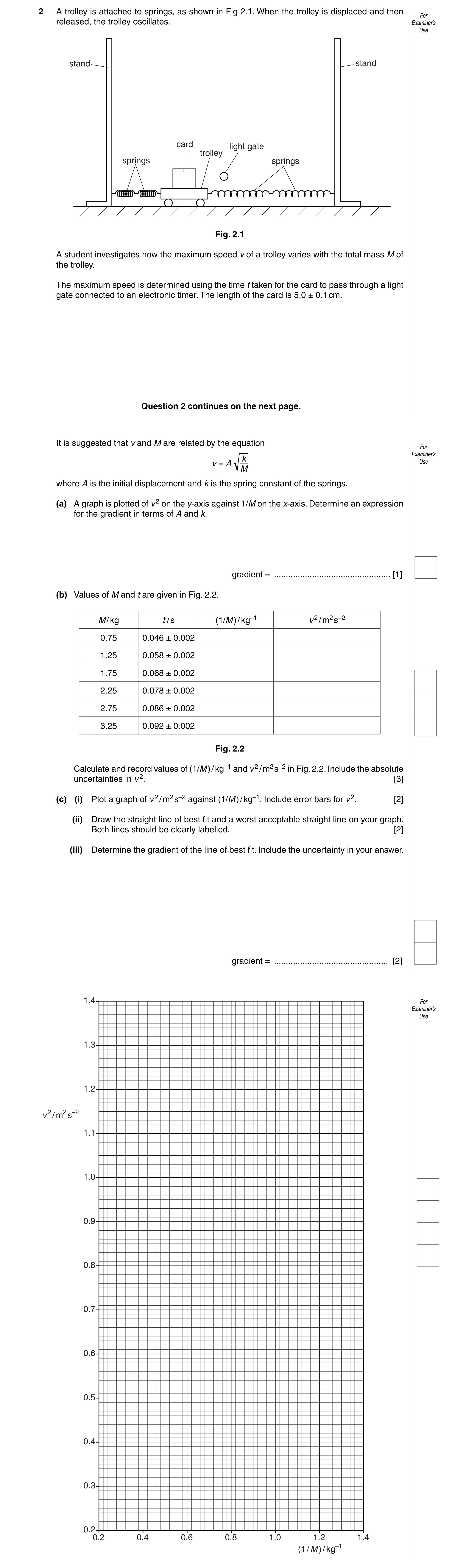
2 A trolley is attached to springs, as shown in Fig 2.1. When the trolley is displaced and then For released, the trolley oscillates. Examiner’s Use stand stand card light gate trolley springs springs Fig. 2.1 A student investigates how the maximum speed v of a trolley varies with the total mass M of the trolley. The maximum speed is determined using the time t taken for the card to pass through a light gate connected to an electronic timer. The length of the card is 5.0 ± 0.1 cm. Question 2 continues on the next page. It is suggested that v and M are related by the equation For Examiner’s k Use v = A M where A is the initial displacement and k is the spring constant of the springs. (a) A graph is plotted of v 2 on the y-axis against 1/M on the x-axis. Determine an expression for the gradient in terms of A and k. gradient = … [1] (b) Values of M and t are given in Fig. 2.2. M / kg t / s (1/M ) / kg–1 v 2 / m2 s–2 0.75 0.046 ± 0.002 1.25 0.058 ± 0.002 1.75 0.068 ± 0.002 2.25 0.078 ± 0.002 2.75 0.086 ± 0.002 3.25 0.092 ± 0.002 Fig. 2.2 Calculate and record values of (1/M ) / kg–1 and v 2 / m2 s–2 in Fig. 2.2. Include the absolute uncertainties in v 2. [3] (c) (i) Plot a graph of v 2 / m2 s–2 against (1/M ) / kg–1. Include error bars for v 2. [2] (ii) Draw the straight line of best fit and a worst acceptable straight line on your graph. Both lines should be clearly labelled. [2] (iii) Determine the gradient of the line of best fit. Include the uncertainty in your answer. gradient = … [2] 1.4 For Examiner’s Use 1.3 1.2 v 2 / m2 s–2 1.1 1.0 0.9 0.8 0.7 0.6 0.5 0.4 0.3 0.2 0.2 0.4 0.6 0.8 1.0 1.2 1.4 (1 / M ) / kg–1
10 marks
Mark scheme: 2 Analysis, conclusions and evaluation (15 marks) Part Mark Expected Answer Additional Guidance (a) A1 Gradient = kA2 (b) T1 T1 must be values in 1/M. Ignore row 2. T2 1.3 or 1.33 1.2 0.8(0)(0)(0) 0.74 T2 must be to 2 s.f. or 3 s.f. 0.571 or 0.54 or 0.55 0.5714 0.444 or 0.41 or 0.411 0.4444 or 0.410 0.364 or 0.34 0.3636 0.308 or 0.29 or 0.30 0.3077 U1 From ± 0.2 or ± 0.15 to ± 0.02 or Allow more than one significant figure. ± 0.03 Do not allow ± 0.1 for row 1. (c) (i) G1 Six points plotted correctly Must be within half a small square. Penalise ‘blobs’. Ecf allowed from table. U2 All error bars in v2 plotted Must be accurate within half a small square. correctly (c) (ii) G2 Line of best fit There must be a balance of points about the line of best fit – examiner judgement. Allow ecf from points plotted incorrectly. G3 Worst acceptable straight line. Line should be clearly labelled or dashed. Should Steepest or shallowest possible pass from top of top error bar to bottom of bottom line that passes through all the error bar or bottom of top error bar to top of bottom error bars. error bar. Mark scored only if error bars are plotted. (c) (iii) C1 Gradient of best fit line The triangle used should be at least half the length of the drawn line. Check the read offs. Work to half a small square. Do not penalise POT. Should be about 0.9. U3 Uncertainty in gradient Method of determining absolute uncertainty. Difference in worst gradient and gradient. (d) (i) C2 k = gradient / A2 Should be about 22. = gradient / 0.04 C3 N m–1 Allow kg s–2 (d) (ii) U4 Percentage uncertainty in k ∆m ∆A ∆m × 100 + 2 × × 100 = × 100 + 5% m A m GCE AS/A LEVEL – October/November 2012 9702 53 (e) C4 v in the range 0.534 to 0.559 For 2 s.f. 0.53 to 0.56 and given to 2 or 3 s.f. U5 Uncertainty in v [Total: 15] Uncertainties in Question 2 (c) (iii) Gradient [U3] Uncertainty = gradient of line of best fit – gradient of worst acceptable line Uncertainty = ½ (steepest worst line gradient – shallowest worst line gradient) (d) (ii) [U4] ∆m ∆A ∆m Percentage uncertainty = × 100 + 2 × × 100 = × 100 + 5% m A m max m Maximum k = (min A ) 2 min m Minimum k = (max A ) 2 ∆k 1 (max k − min k ) Percentage uncertainty = × 100 = 2 × 100 k k (e) [U5] ∆A 1 ∆k Percentage uncertainty = × 100 + 2 × × 100 A k Absolute uncertainty = v × percentage uncertainty/100 max k Maximum v = max A× 0.75 min k Minimum v = min A × 0.75 Absolute uncertainty = max v – v or v – min v or 12 (max v − min v )
This question in 9702/53 Oct/Nov 2012
Q6 · A ball rolls forwards and backwards on a curved track as shown in Fig 9702/51 May/June 2014
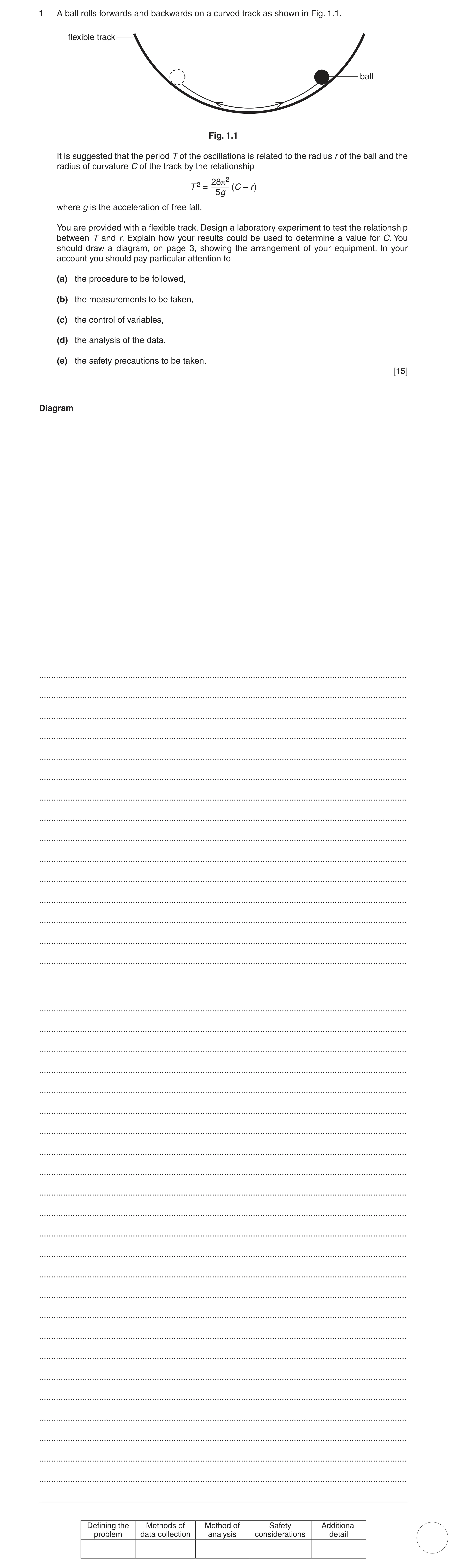
1 A ball rolls forwards and backwards on a curved track as shown in Fig. 1.1. flexible track ball Fig. 1.1 It is suggested that the period T of the oscillations is related to the radius r of the ball and the radius of curvature C of the track by the relationship 2 28p2 T = (C – r ) 5g where g is the acceleration of free fall. You are provided with a flexible track. Design a laboratory experiment to test the relationship between T and r. Explain how your results could be used to determine a value for C. You should draw a diagram, on page 3, showing the arrangement of your equipment. In your account you should pay particular attention to (a) the procedure to be followed, (b) the measurements to be taken, (c) the control of variables, (d) the analysis of the data, (e) the safety precautions to be taken. [15] Diagram … … … … … … … … … … … … … … … … … … … … … … … … … … … … … … … … … … … … … … … Defining the Methods of Method of Safety Additional problem data collection analysis considerations detail
15 marks
Mark scheme: 1 Planning (15 marks) Defining the problem (3 marks) P r is the independent variable or vary r. [1] P T (or t) is the dependent variable or measure T (or t). [1] P Keep the radius of curvature (of the track) or C constant (or radius of track constant). Do not allow “use same track”. [1] Methods of data collection (5 marks) M Diagram showing ball in a (curved) track with supports for track, e.g. retort stands. Minimum of two labels (from ball, track, supports; not stopwatch, bench, micrometer). Supports making contact with track higher than ball / at least half way up. [1] M Measure time using stopwatch or light gates and timer or datalogger with motion sensor. Detail needed for video camera. [1] M Use many oscillations (at least 10 or at least 10 s of timing) and determine T = t / n. [1] M Measure diameter (radius) of ball with a micrometer / vernier calipers. Do not allow travelling microscope. [1] M radius = diameter / 2. [1] Method of analysis (2 marks) A Plot a graph of T 2 against r (or r against T 2) Do not allow log graphs. [1] 5 g y − intercept A C = y-intercept × = (or for r against T 2, C = y-intercept) [1] 2 gradient 28 π Safety considerations (1 mark) S Precaution linked to ball escaping on to floor, e.g. use barrier / safety screen / sand tray to prevent balls rolling on to floor. [1] GCE AS/A LEVEL – May/June 2014 9702 51 Additional detail (4 marks) D Relevant points might include [4] 1 Add weights to / G-clamp retort stands 2 Keep the material / density of the ball constant 3 Use of fiducial marker near centre of track / mark on the track 4 Clean track / balls. Do not allow oil the track. 5 Repeat measurements of t (for each ball) and average 6 Repeat measurement for d (or r) and average 7 Relationship is valid if straight line, provided plotted graph is correct 8 Relationship is valid if straight line not passing through origin or has an intercept, provided plotted graph is correct (any quoted expression must be correct, e.g. 28 π 2C y-intercept = ) 5 g Do not allow vague computer methods. [Total: 15] GCE AS/A LEVEL – May/June 2014 9702 51
This question in 9702/51 May/June 2014
Q7 · A student is investigating simple harmonic motion using an electric vibrator 9702/51 May/June 2015
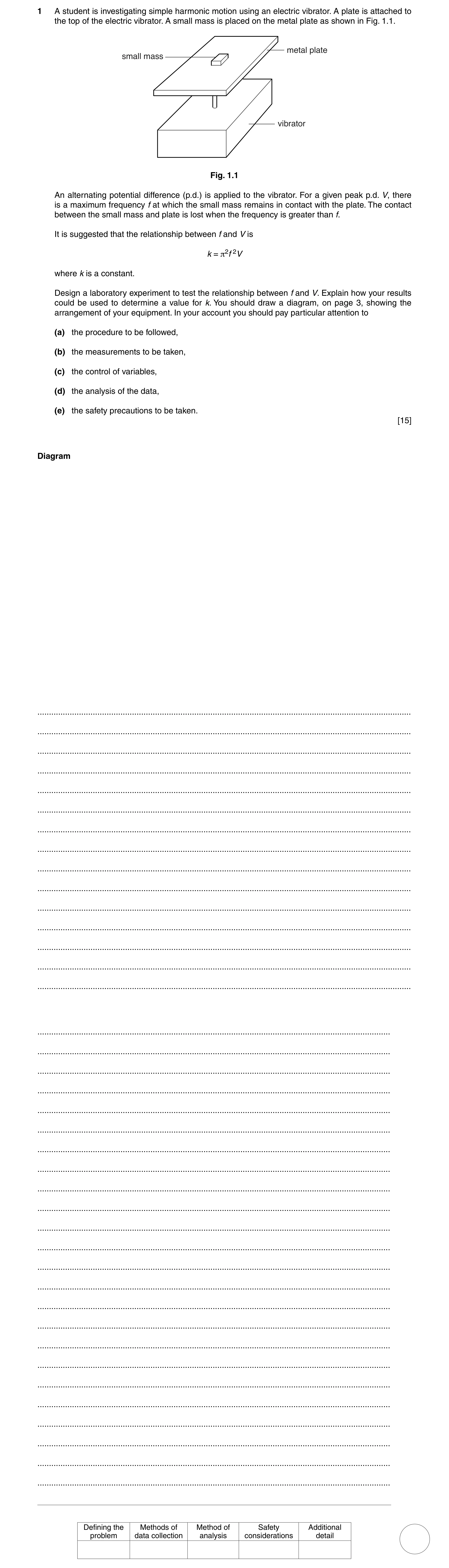
1 A student is investigating simple harmonic motion using an electric vibrator. A plate is attached to the top of the electric vibrator. A small mass is placed on the metal plate as shown in Fig. 1.1. metal plate small mass vibrator Fig. 1.1 An alternating potential difference (p.d.) is applied to the vibrator. For a given peak p.d. V, there is a maximum frequency f at which the small mass remains in contact with the plate. The contact between the small mass and plate is lost when the frequency is greater than f. It is suggested that the relationship between f and V is k = π2f 2V where k is a constant. Design a laboratory experiment to test the relationship between f and V. Explain how your results could be used to determine a value for k. You should draw a diagram, on page 3, showing the arrangement of your equipment. In your account you should pay particular attention to (a) the procedure to be followed, (b) the measurements to be taken, (c) the control of variables, (d) the analysis of the data, (e) the safety precautions to be taken. [15] Diagram … … … … … … … … … … … … … … … … … … … … … … … … … … … … … … … … … … … … … … … Defining the Methods of Method of Safety Additional problem data collection analysis considerations detail
15 marks
Mark scheme: 1 Planning (15 marks) Defining the problem (3 marks) P V is the independent variable, or vary V and f is the dependent variable, or measure f. Or f is the independent variable, or vary f and V is the dependent variable, or measure V. [1] P Change f (allow V) until the mass leaves/gap between plate. [1] P Keep the position of the mass constant. (Do not allow keep mass constant.) [1] Methods of data collection (5 marks) M Labelled diagram showing signal generator/a.c. supply connected to vibrator with two wires with mass on plate. At least two labels needed. [1] M Voltmeter/c.r.o. connected in parallel with vibrator in a workable circuit. [1] M Measure f or T from signal generator/c.r.o. (Allow detailed use of motion sensor/stroboscope.) [1] M Detail regarding mass leaving the plate: listen to noise, look for gap. [1] M Repeat each experiment for the same value of V (allow f if consistent with above) and average. [1] Method of analysis (2 marks) Plot a graph of: f 2 1 / V f 1 / V lg V lg f A against against against against against against 1 / V f 2 1 / V f lg f lg V or or or or V 1 / f 2 V 1 / f against against against against [1] 1 / f 2 V 1 / f V k = π 2 k = π 2 k = k = A k = π 2 × 10 c k = π 2 × 10 2 c [1] 2 2 gradient × π 2 × π 2 gradient gradient gradient Safety considerations (1 mark) S Precaution linked to mass leaving vibrating plate, e.g. use safety screen/goggles/sand tray. [1] Additional detail (4 marks) D Relevant points might include [4] 1 Wait for vibrator to oscillate evenly 2 Method to determine period of oscillation from c.r.o., i.e. one time period × time-base 3 Method to determine f from c.r.o. having determined T, i.e. f = 1 / T 4 Method to determine V from c.r.o, i.e. amplitude (height) × y-gain 5 Relationship is valid if the graph is a straight line passing through the origin [For lg – lg graph the gradient must be correct (–2 or –0.5)] 6 Determine f (allow V if consistent with above) by increasing and decreasing V or f 7 Clean surfaces of metal plate/small mass 8 Spirit level to keep plate horizontal/eye level to look for gap Do not allow vague computer methods.
This question in 9702/51 May/June 2015
Q8 · A student is investigating simple harmonic motion using an electric vibrator 9702/53 May/June 2015
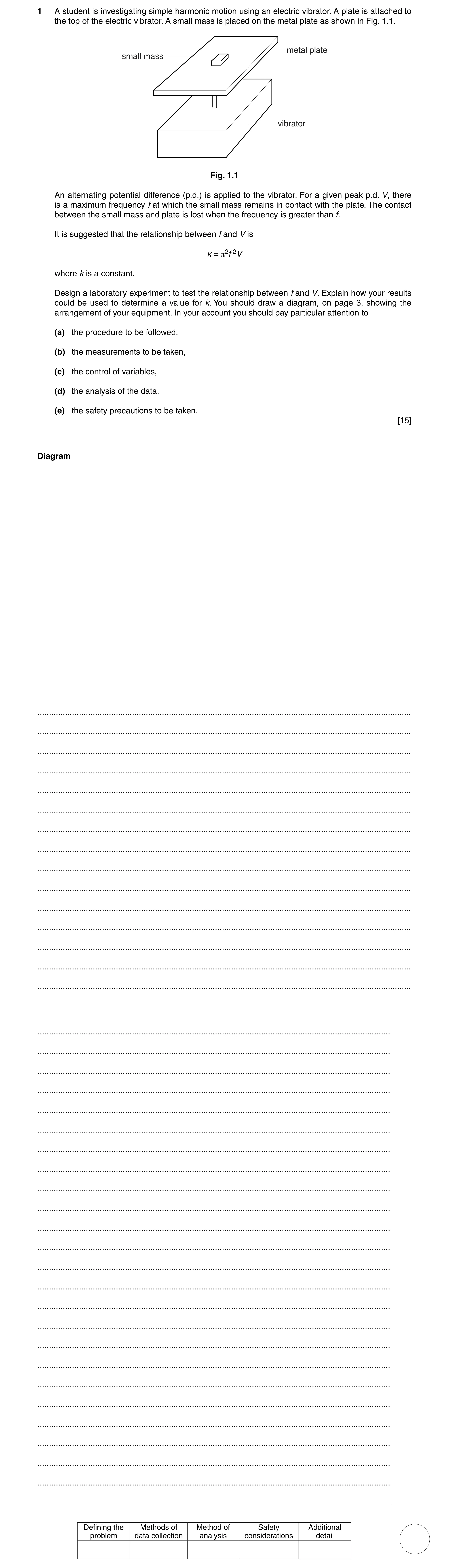
1 A student is investigating simple harmonic motion using an electric vibrator. A plate is attached to the top of the electric vibrator. A small mass is placed on the metal plate as shown in Fig. 1.1. metal plate small mass vibrator Fig. 1.1 An alternating potential difference (p.d.) is applied to the vibrator. For a given peak p.d. V, there is a maximum frequency f at which the small mass remains in contact with the plate. The contact between the small mass and plate is lost when the frequency is greater than f. It is suggested that the relationship between f and V is k = π2f 2V where k is a constant. Design a laboratory experiment to test the relationship between f and V. Explain how your results could be used to determine a value for k. You should draw a diagram, on page 3, showing the arrangement of your equipment. In your account you should pay particular attention to (a) the procedure to be followed, (b) the measurements to be taken, (c) the control of variables, (d) the analysis of the data, (e) the safety precautions to be taken. [15] Diagram … … … … … … … … … … … … … … … … … … … … … … … … … … … … … … … … … … … … … … … Defining the Methods of Method of Safety Additional problem data collection analysis considerations detail
15 marks
Mark scheme: 1 Planning (15 marks) Defining the problem (3 marks) P V is the independent variable, or vary V and f is the dependent variable, or measure f. Or f is the independent variable, or vary f and V is the dependent variable, or measure V. [1] P Change f (allow V) until the mass leaves/gap between plate. [1] P Keep the position of the mass constant. (Do not allow keep mass constant.) [1] Methods of data collection (5 marks) M Labelled diagram showing signal generator/a.c. supply connected to vibrator with two wires with mass on plate. At least two labels needed. [1] M Voltmeter/c.r.o. connected in parallel with vibrator in a workable circuit. [1] M Measure f or T from signal generator/c.r.o. (Allow detailed use of motion sensor/stroboscope.) [1] M Detail regarding mass leaving the plate: listen to noise, look for gap. [1] M Repeat each experiment for the same value of V (allow f if consistent with above) and average. [1] Method of analysis (2 marks) Plot a graph of: f 2 1 / V f 1 / V lg V lg f A against against against against against against 1 / V f 2 1 / V f lg f lg V or or or or V 1 / f 2 V 1 / f against against against against [1] 1 / f 2 V 1 / f V k = π 2 k = π 2 k = k = A k = π 2 × 10 c k = π 2 × 10 2 c [1] 2 2 gradient × π 2 × π 2 gradient gradient gradient Safety considerations (1 mark) S Precaution linked to mass leaving vibrating plate, e.g. use safety screen/goggles/sand tray. [1] Additional detail (4 marks) D Relevant points might include [4] 1 Wait for vibrator to oscillate evenly 2 Method to determine period of oscillation from c.r.o., i.e. one time period × time-base 3 Method to determine f from c.r.o. having determined T, i.e. f = 1 / T 4 Method to determine V from c.r.o, i.e. amplitude (height) × y-gain 5 Relationship is valid if the graph is a straight line passing through the origin [For lg – lg graph the gradient must be correct (–2 or –0.5)] 6 Determine f (allow V if consistent with above) by increasing and decreasing V or f 7 Clean surfaces of metal plate/small mass 8 Spirit level to keep plate horizontal/eye level to look for gap Do not allow vague computer methods.
This question in 9702/53 May/June 2015
Q9 · A student is investigating the oscillations of a mass attached to an arrangement of… 9702/52 May/June 2019
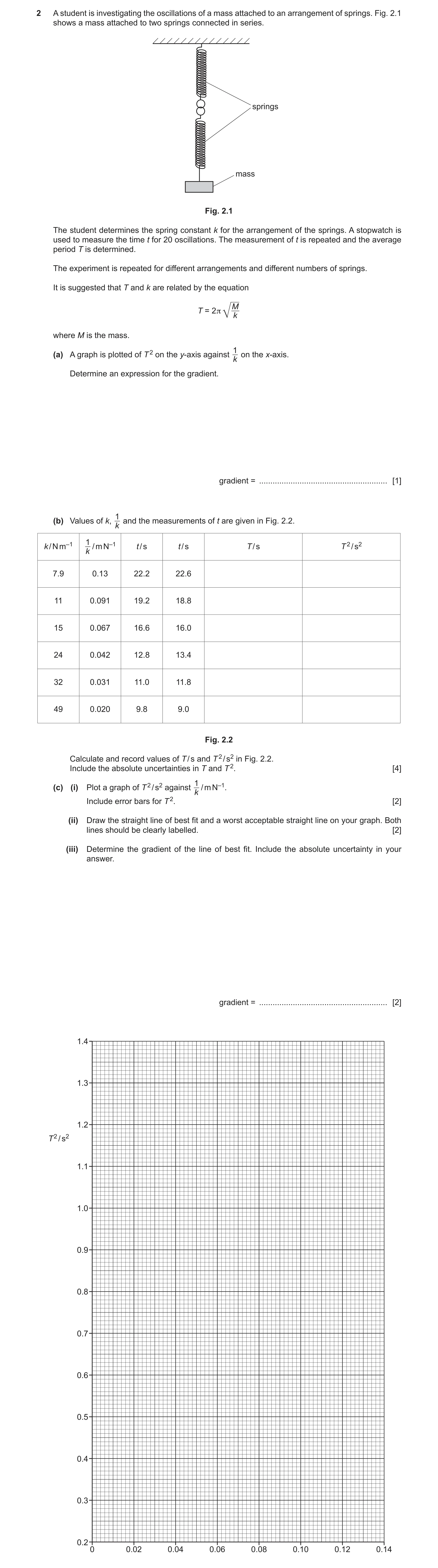
2 A student is investigating the oscillations of a mass attached to an arrangement of springs. Fig. 2.1 shows a mass attached to two springs connected in series. springs mass Fig. 2.1 The student determines the spring constant k for the arrangement of the springs. A stopwatch is used to measure the time t for 20 oscillations. The measurement of t is repeated and the average period T is determined. The experiment is repeated for different arrangements and different numbers of springs. It is suggested that T and k are related by the equation M T = 2 π k where M is the mass. 2 1 (a) A graph is plotted of T on the y-axis against on the x-axis. k Determine an expression for the gradient. gradient = … [1] 1 (b) Values of k, and the measurements of t are given in Fig. 2.2. k 1 2k / N m–1 / m N–1 t / s t / s T / s T / s2 k 7.9 0.13 22.2 22.6 11 0.091 19.2 18.8 15 0.067 16.6 16.0 24 0.042 12.8 13.4 32 0.031 11.0 11.8 49 0.020 9.8 9.0 Fig. 2.2 Calculate and record values of T / s and T 2 / s2 in Fig. 2.2. Include the absolute uncertainties in T and T 2. [4] 2 1 (c) (i) Plot a graph of T / s2 against / m N–1. k Include error bars for T 2. [2] (ii) Draw the straight line of best fit and a worst acceptable straight line on your graph. Both lines should be clearly labelled. [2] (iii) Determine the gradient of the line of best fit. Include the absolute uncertainty in your answer. gradient = … [2]
11 marks
Mark scheme: 2(a) 1 2(b) T / s T2 / s2 1.12 or 1.120 1.25 or 1.254 0.950 or 0.9500 0.903 or 0.9025 0.815 or 0.8150 0.664 or 0.6642 0.655 or 0.6550 0.429 or 0.4290 0.570 or 0.5700 0.325 or 0.3249 0.47 or 0.470 0.22 or 0.221 Values of T as above. 1 Values of T2 as above. 1 Uncertainties in T increase from ±0.01 to ±0.02. 1 Uncertainties in T2 about ±0.02. 1 2(c)(i) Six points plotted correctly. Must be accurate to the nearest half a small square. Diameter of points must be less than half a small square. 1 Error bars in T2 plotted correctly. All error bars to be plotted. Length of bar must be accurate to less than half a small square and symmetrical. 1 2(c)(ii) Line of best fit drawn. If points are plotted correctly then lower end of line should pass between (0.048, 0.5) and (0.052, 0.5) and upper end of line should pass between (0.098, 1.0) and (0.104, 1.0). 1 Worst acceptable line drawn (steepest or shallowest possible line that passes through all the error bars). All error bars must be plotted. 1 Question Answer Marks 2(c)(iii) Gradient determined with clear substitution of points from the line of best fit into ∆y / ∆x. Distance between points must be at least half the length of the drawn line. 1 uncertainty = gradient of line of best fit – gradient of worst acceptable line or uncertainty = ½ (steepest worst line gradient – shallowest worst line gradient) 1 2(d)(i) M determined from gradient and given to 2 or 3 significant figures and with correct unit. 2 gradient 39.478 4 M = = π (c)(iii) 1 2(d)(ii) % uncertainty in M = % uncertainty in gradient 1 Question Answer Marks 2(e) k calculated. Correct substitution of numbers required. 2 2 2 2 4 4 6.3165 2.5 M k T π π = = × (d)(i) or (d)(i) or 2 2 gradient 6.25 2.5 k T = = (c)(iii) (c)(iii) or 1 Absolute uncertainty in k. Correct substitution of numbers required. Using M: uncertainty in 2 M T k k M T ∆ ∆ = + × × uncertainty in 0.008 100 k k = + × (d)(ii) 2 2 2 2 4 max 4 min max min min max M M k k T T π × π × = = or Using gradient: gradient uncertainty in 0.008 gradient k k ∆ = + × 2 2 maxgradient mingradient max min min max k k T T = = or 1
This question in 9702/52 May/June 2019
Q10 · A student investigates the vertical oscillations of a solid cylinder which floats in… 9702/52 Feb/March 2021
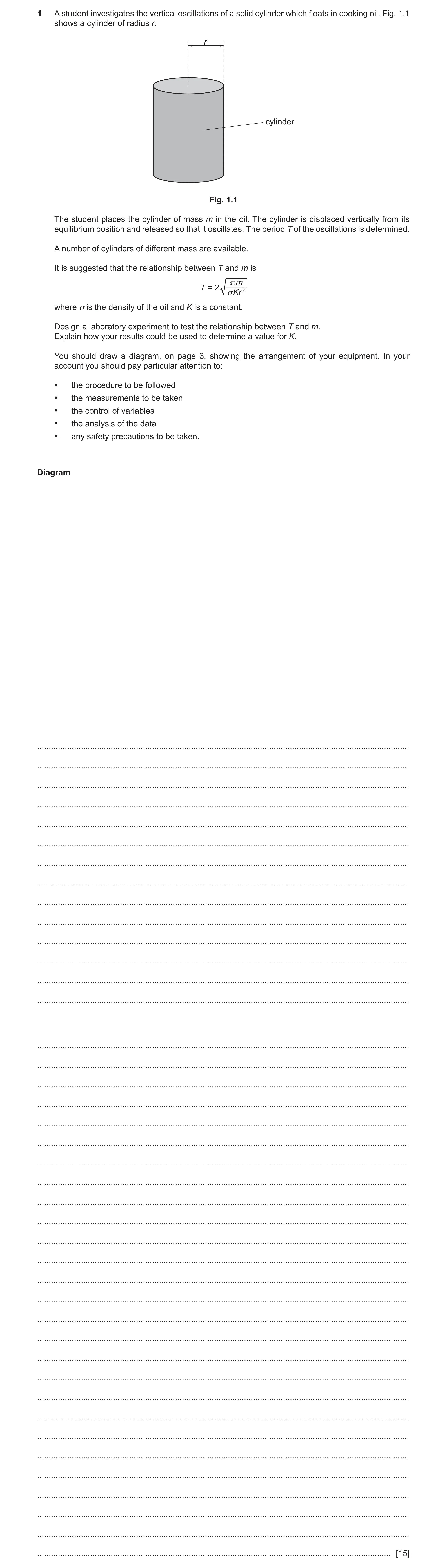
1 A student investigates the vertical oscillations of a solid cylinder which floats in cooking oil. Fig. 1.1 shows a cylinder of radius r. r cylinder Fig. 1.1 The student places the cylinder of mass m in the oil. The cylinder is displaced vertically from its equilibrium position and released so that it oscillates. The period T of the oscillations is determined. A number of cylinders of different mass are available. It is suggested that the relationship between T and m is π m T = 2 2 σ Kr where σ is the density of the oil and K is a constant. Design a laboratory experiment to test the relationship between T and m. Explain how your results could be used to determine a value for K. You should draw a diagram, on page 3, showing the arrangement of your equipment. In your account you should pay particular attention to: • the procedure to be followed • the measurements to be taken • the control of variables • the analysis of the data • any safety precautions to be taken. Diagram … … … … … … … … … … … … … … … … … … … … … … … … … … … … … … … … … … … … … … … … … [15]
15 marks
Mark scheme: 1 Defining the problem Mass of cylinder m is the independent variable and period T is the dependent variable, or vary mass of cylinder m and measure period T. 1 Keep radius of cylinder constant. 1 Methods of data collection Labelled diagram of workable experiment including: • beaker with (cooking) oil on a bench or container supported by stand where stand is on a bench • cylinder partially submerged in (cooking) oil • cylinder and (cooking) oil labelled. 1 Method to determine mass m of cylinder, e.g. use a (top pan) balance. 1 Method to determine period or T, e.g. use a stopwatch / timer to time oscillations. 1 Method to determine diameter of cylinder, e.g. micrometer or calliper 1 Method of Analysis Plots a graph of T2 against m. (Allow other valid graphs, e.g. lg T against lg m) 1 Relationship valid if a straight line passing through the origin is produced. (Allow gradient = 0.5 for log T against log m). 1 σ = × 2 4π gradient K r ( σ × = × 2 y-intercept 2 4π 10 K r for lg T against lg m). 1 Question Answer Marks 1 Additional detail including safety considerations Max 6 6 Use gloves to prevent oil contacting skin / slippery hands OR Perform experiment in a tray to prevent oil spillages. D1 Keep density / temperature of the (cooking) oil constant or keep σ constant. D2 Mass of oil = mass of beaker and oil – mass of beaker and use a measuring cylinder to determine the volume of the oil. Do not accept (calibrated) beaker. D3 Methods to measure volume of oil and determine mass of oil and use equation density σ = mass / volume for measurements. D4 Time n oscillations and divide nT by n where n ⩾ 5. D5 Description of method of counting oscillations with position of fiducial mark / mark on cylinder / beaker / fixed point shown in diagram. D6 Repeat experiment for each value of m and average T. D7 r = diameter / 2 provided diameter measured. D8 Repeat measurements of diameter in different directions and average. D9 Wait for oscillations to become even / steady. D10
This question in 9702/52 Feb/March 2021
 10
10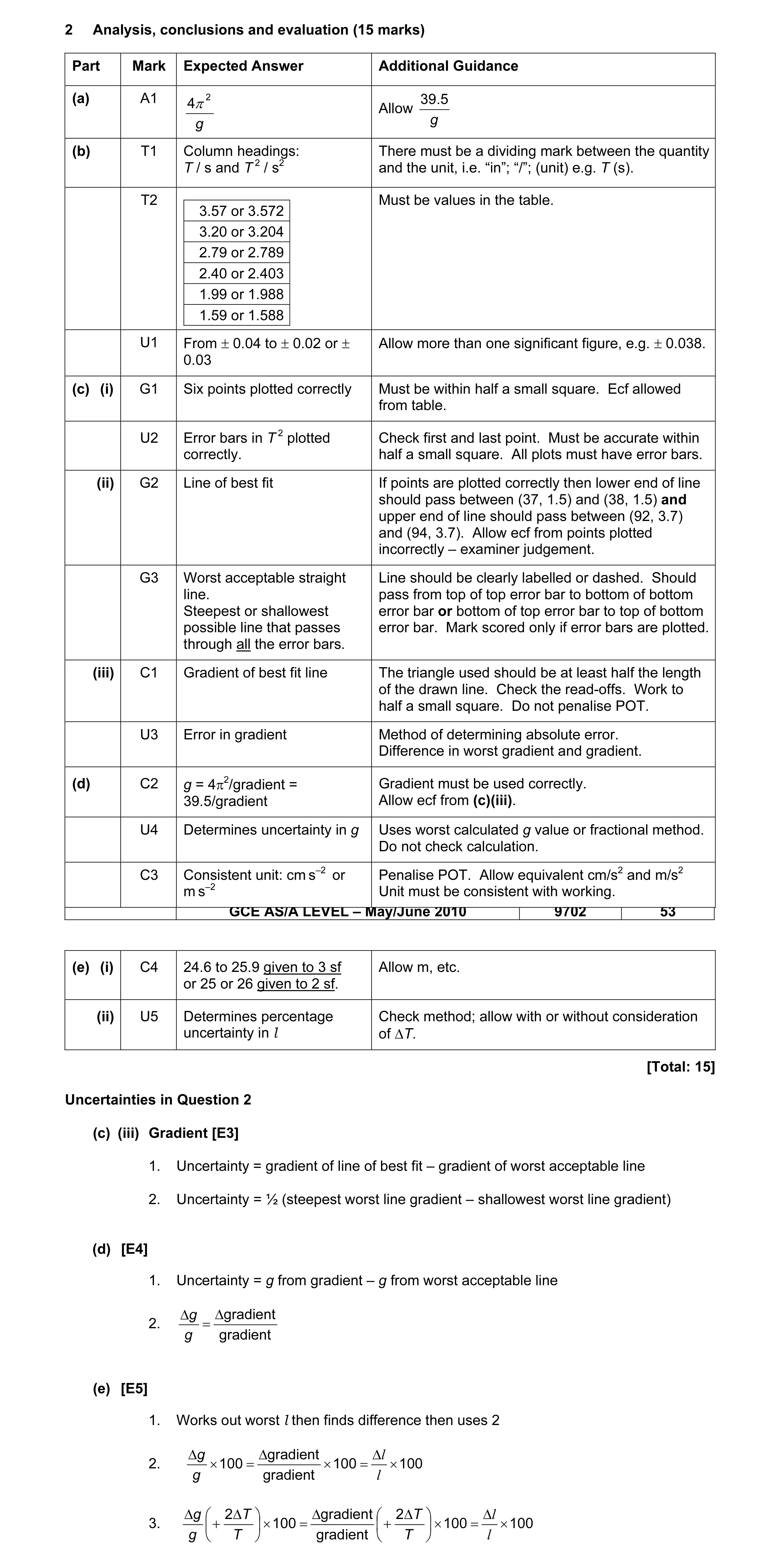 10
10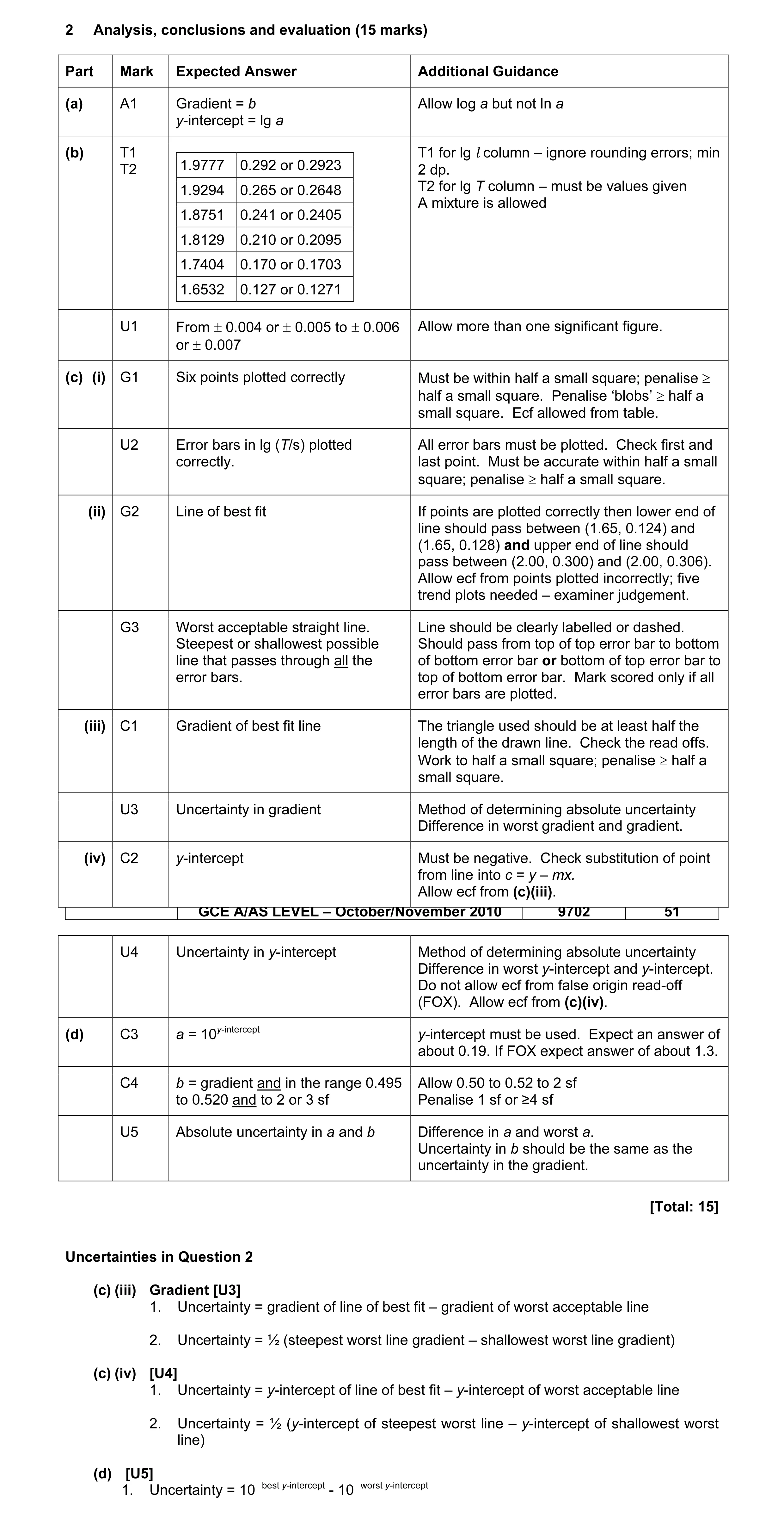 10
10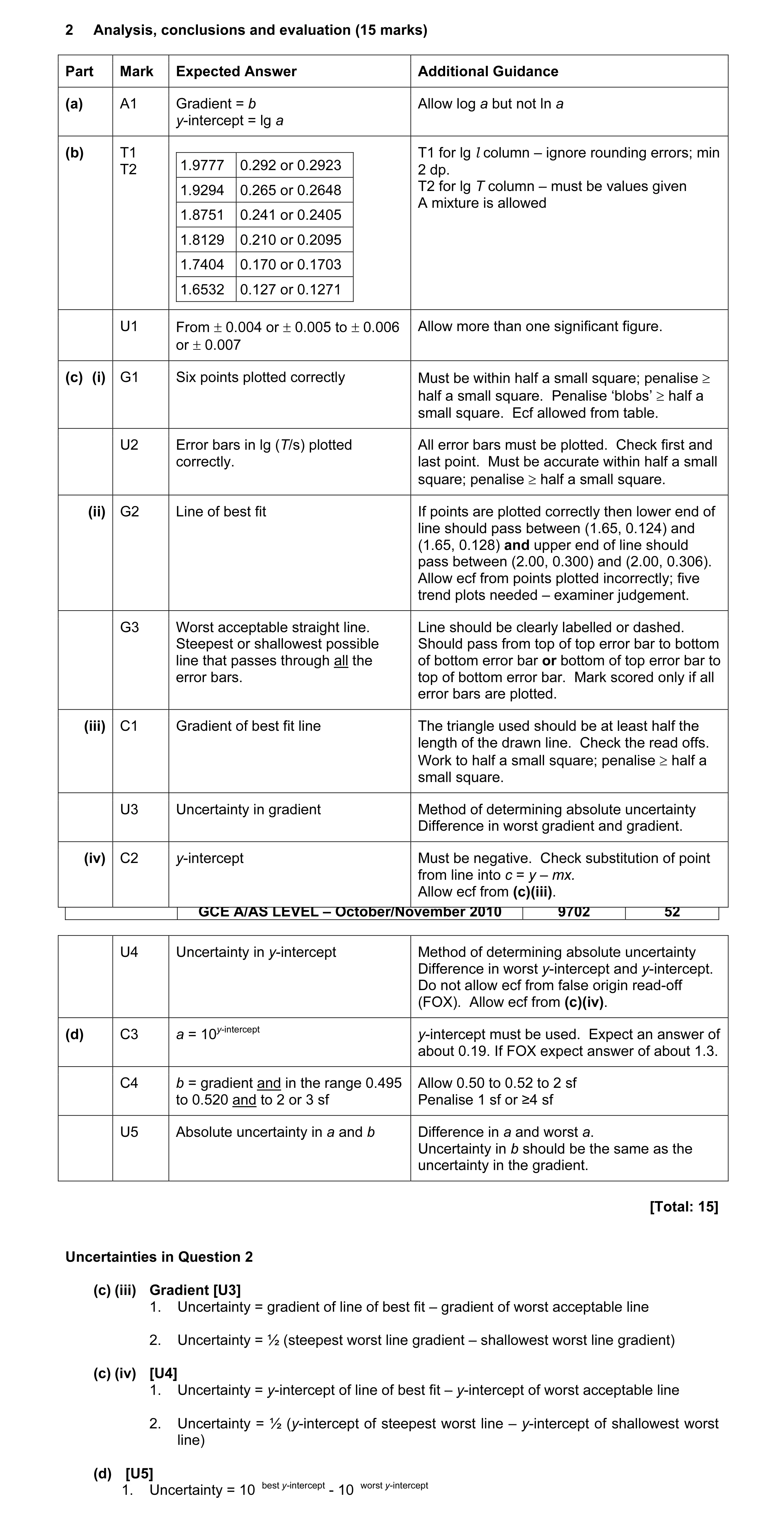 10
10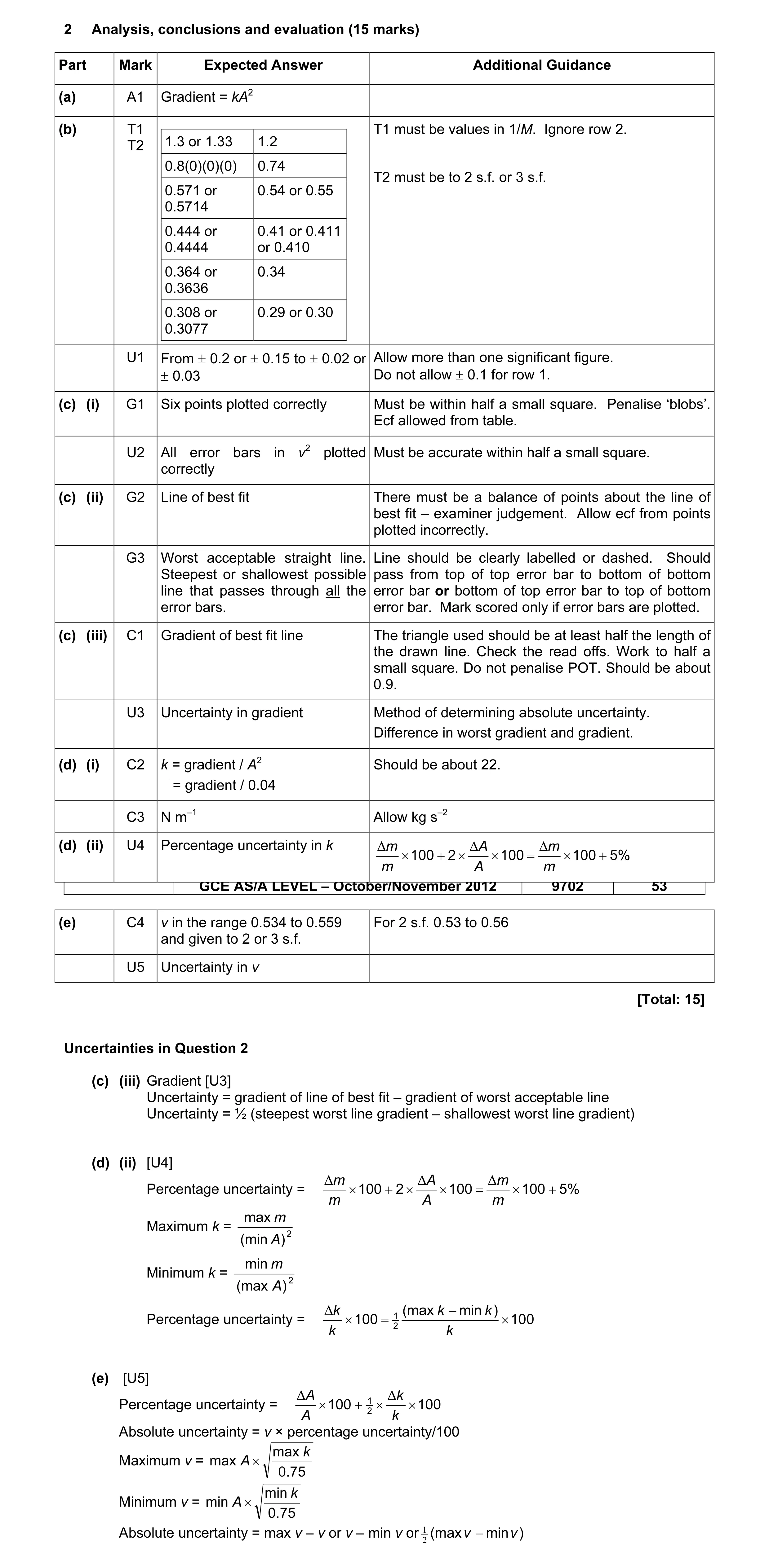 10
10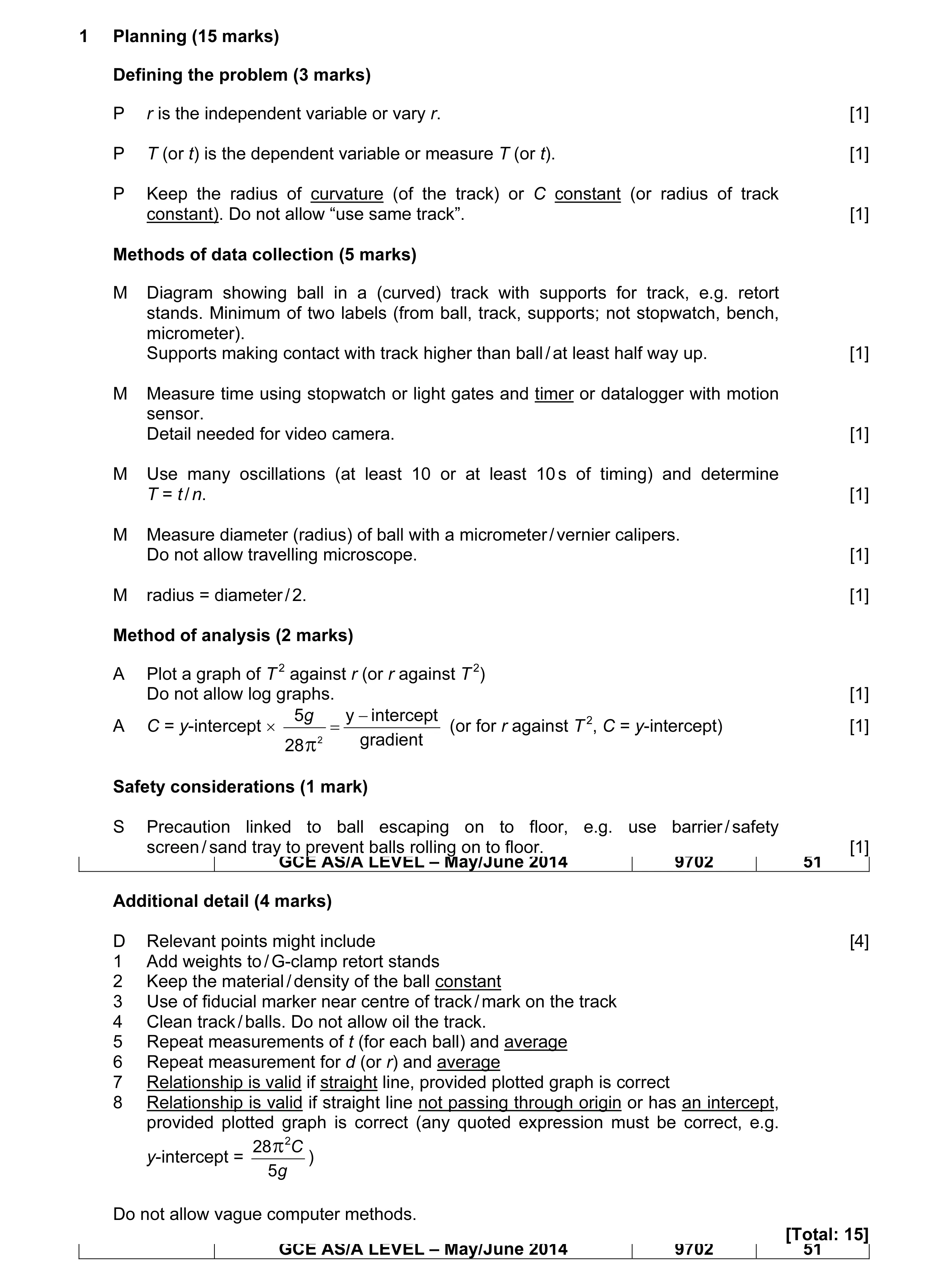 15
15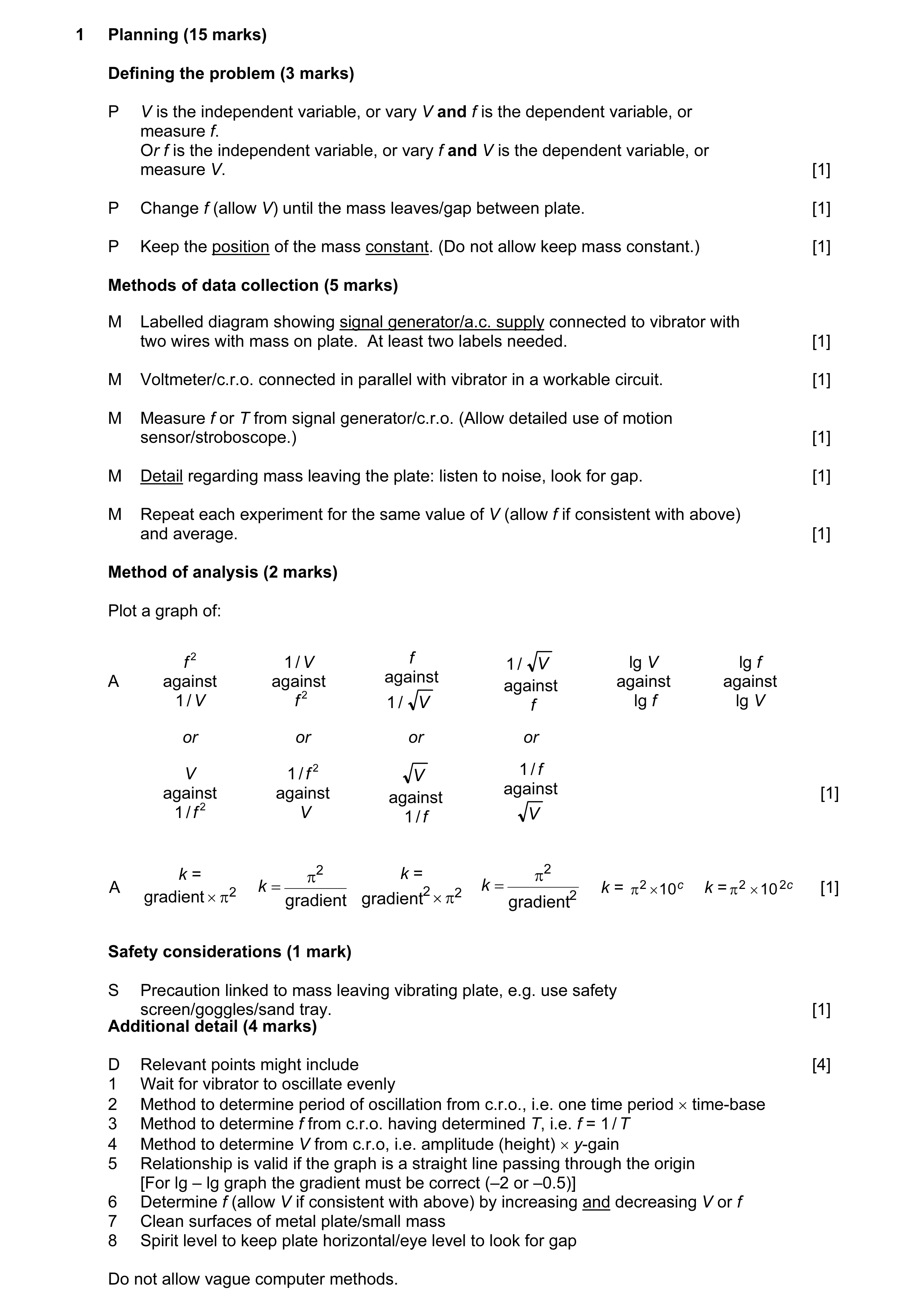 15
15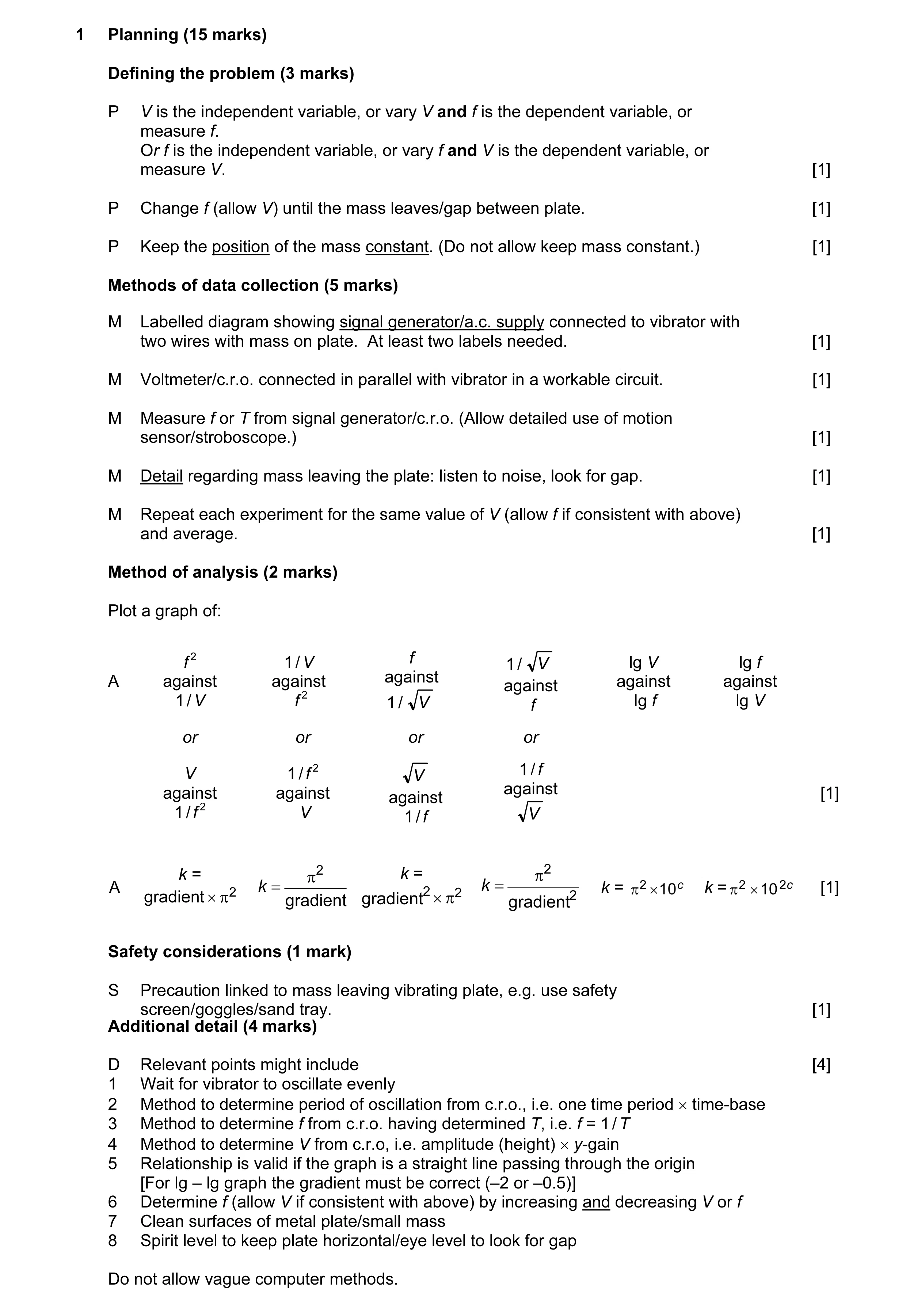 15
15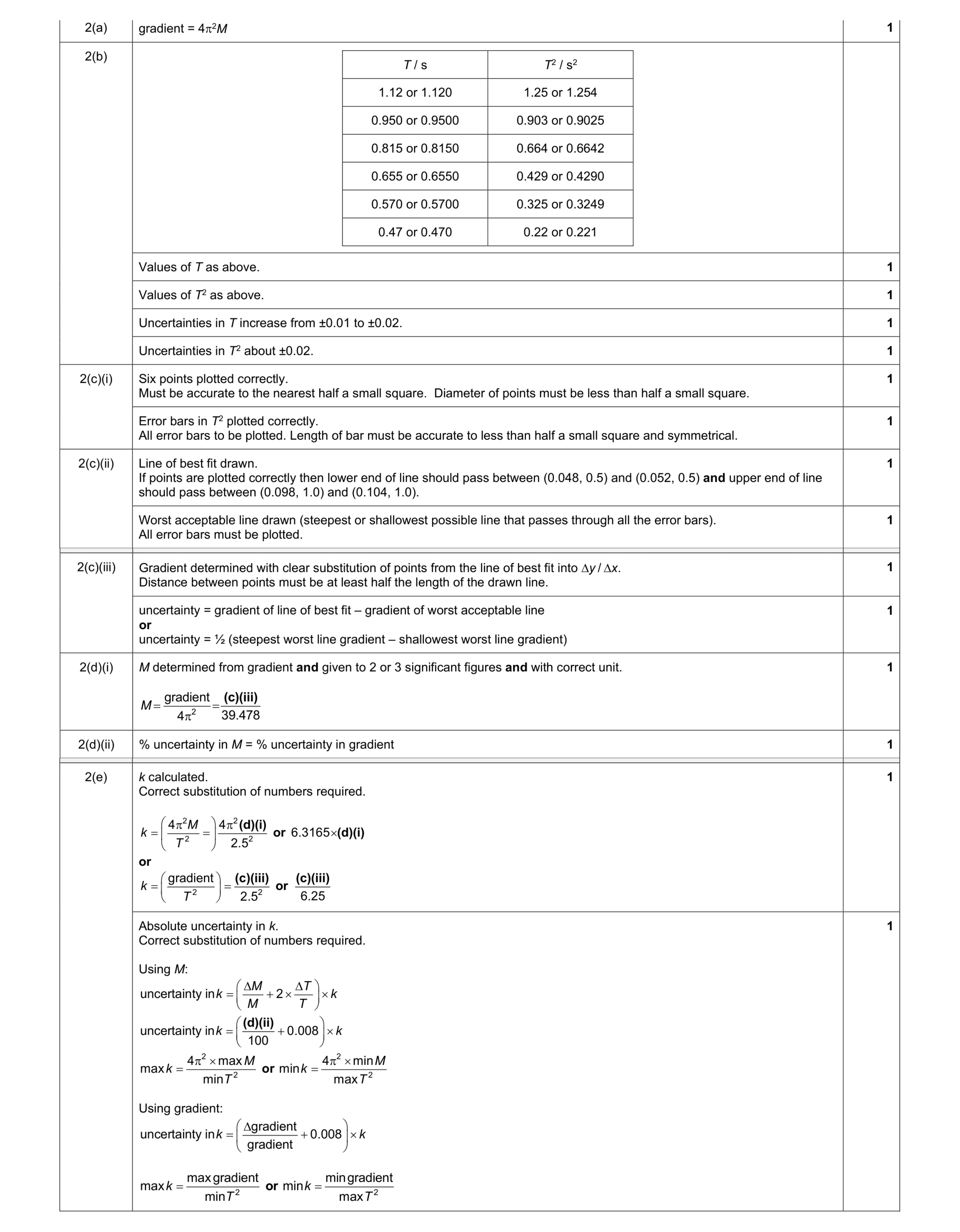 11
11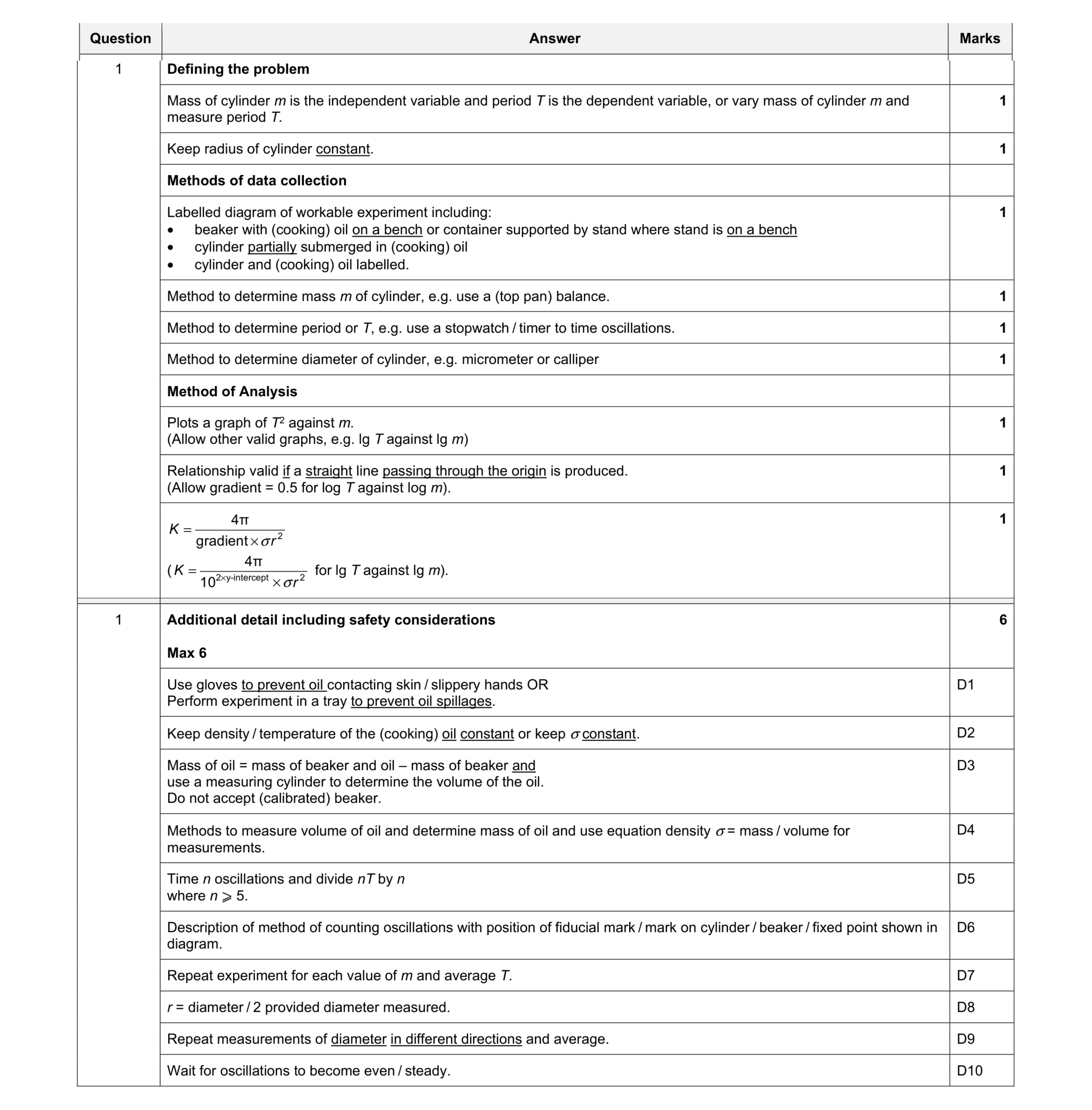 15
15