Cambridge A Level Marine Science 9693 — 2022 May/June Paper 2 · Variant 3

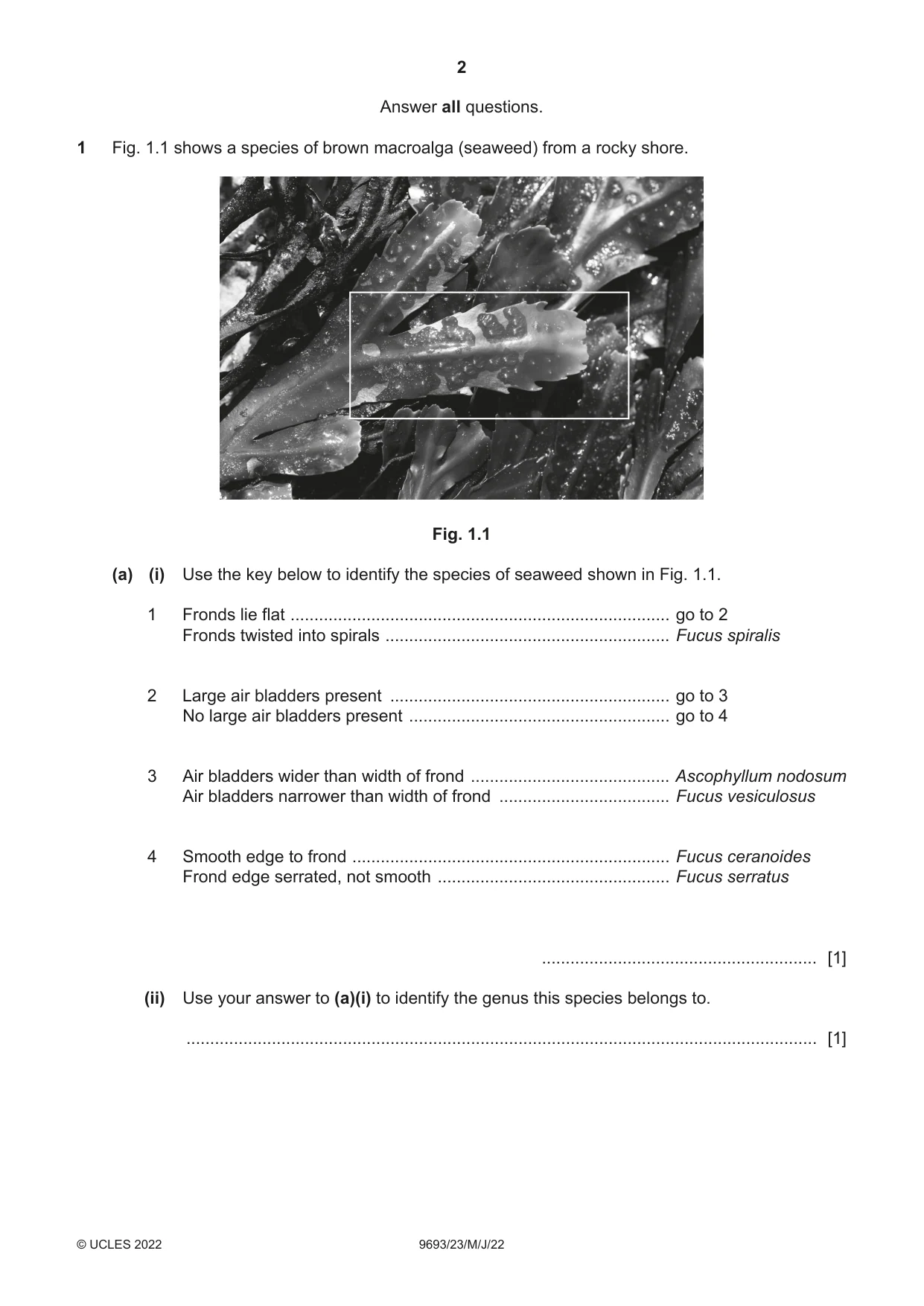
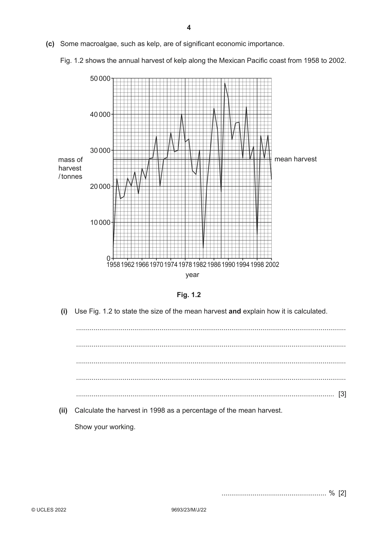
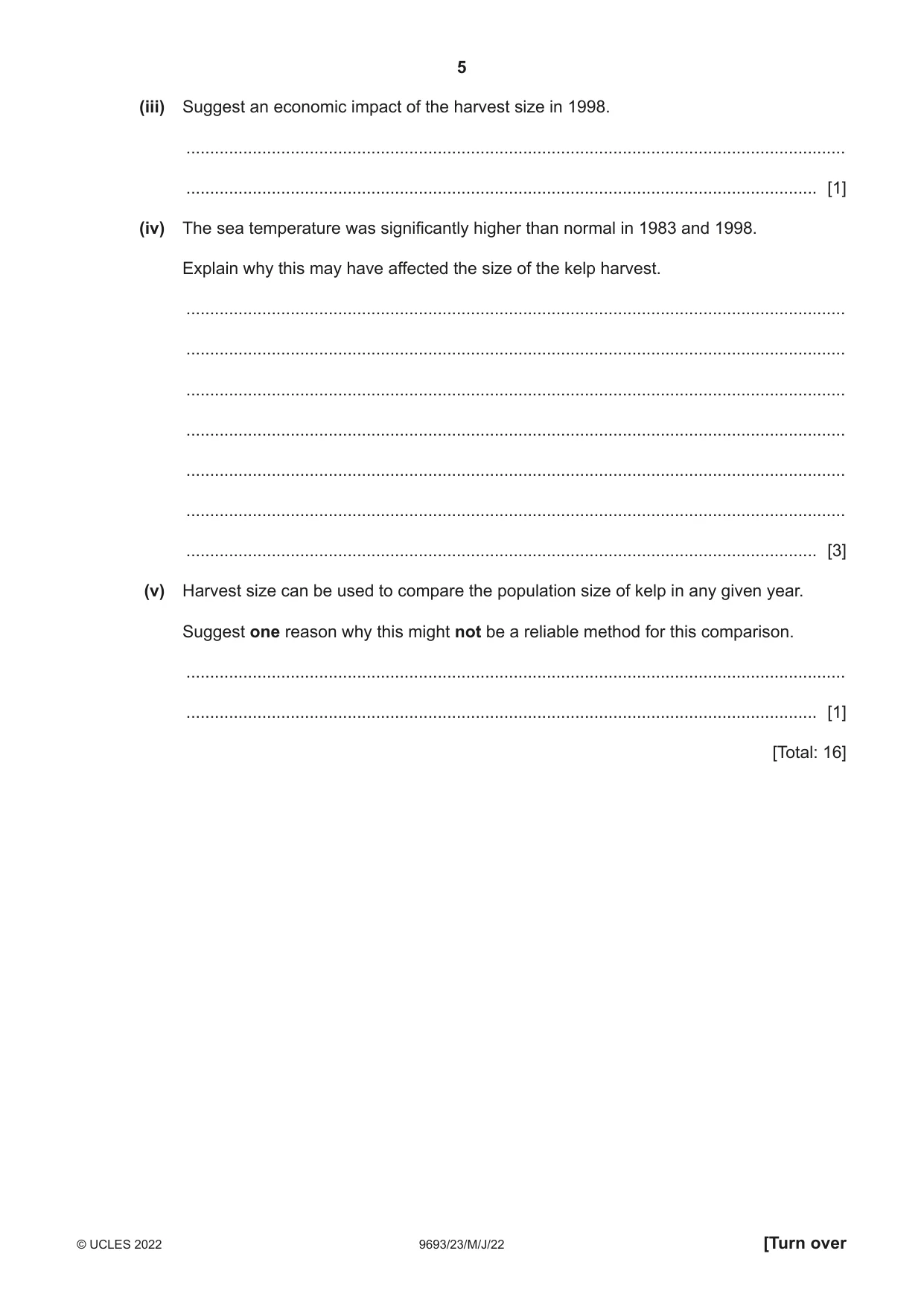
1 Fig. 1.1 shows a species of brown macroalga (seaweed) from a rocky shore. Fig. 1.1 (a) (i) Use the key below to identify the species of seaweed shown in Fig. 1.1. 1 Fronds lie flat ................................................................................ go to 2 Fronds twisted into spirals ............................................................ Fucus spiralis 2 Large air bladders present ........................................................... go to 3 No large air bladders present ....................................................... go to 4 3 Air bladders wider than width of frond .......................................... Ascophyllum nodosum Air bladders narrower than width of frond .................................... Fucus vesiculosus 4 Smooth edge to frond ................................................................... Fucus ceranoides Frond edge serrated, not smooth ................................................. Fucus serratus .......................................................... [1] (ii) Use your answer to (a)(i) to identify the genus this species belongs to. ..................................................................................................................................... [1] (b) Make a large drawing of a frond from the seaweed in Fig. 1.1. Only draw the frond shown inside the white box. Do not label your diagram. [4] (c) Some macroalgae, such as kelp, are of significant economic importance. Fig. 1.2 shows the annual harvest of kelp along the Mexican Pacific coast from 1958 to 2002. 50 000 40 000 30 000 mass of mean harvest harvest / tonnes 20 000 10 000 0 19581962 1966 1970 19741978 19821986199019941998 2002 year Fig. 1.2 (i) Use Fig. 1.2 to state the size of the mean harvest and explain how it is calculated. ........................................................................................................................................... ........................................................................................................................................... ........................................................................................................................................... ........................................................................................................................................... ..................................................................................................................................... [3] (ii) Calculate the harvest in 1998 as a percentage of the mean harvest. Show your working. ...................................................... % [2] (iii) Suggest an economic impact of the harvest size in 1998. ........................................................................................................................................... ..................................................................................................................................... [1] (iv) The sea temperature was significantly higher than normal in 1983 and 1998. Explain why this may have affected the size of the kelp harvest. ........................................................................................................................................... ........................................................................................................................................... ........................................................................................................................................... ........................................................................................................................................... ........................................................................................................................................... ........................................................................................................................................... ..................................................................................................................................... [3] (v) Harvest size can be used to compare the population size of kelp in any given year. Suggest one reason why this might not be a reliable method for this comparison. ........................................................................................................................................... ..................................................................................................................................... [1] [Total: 16]

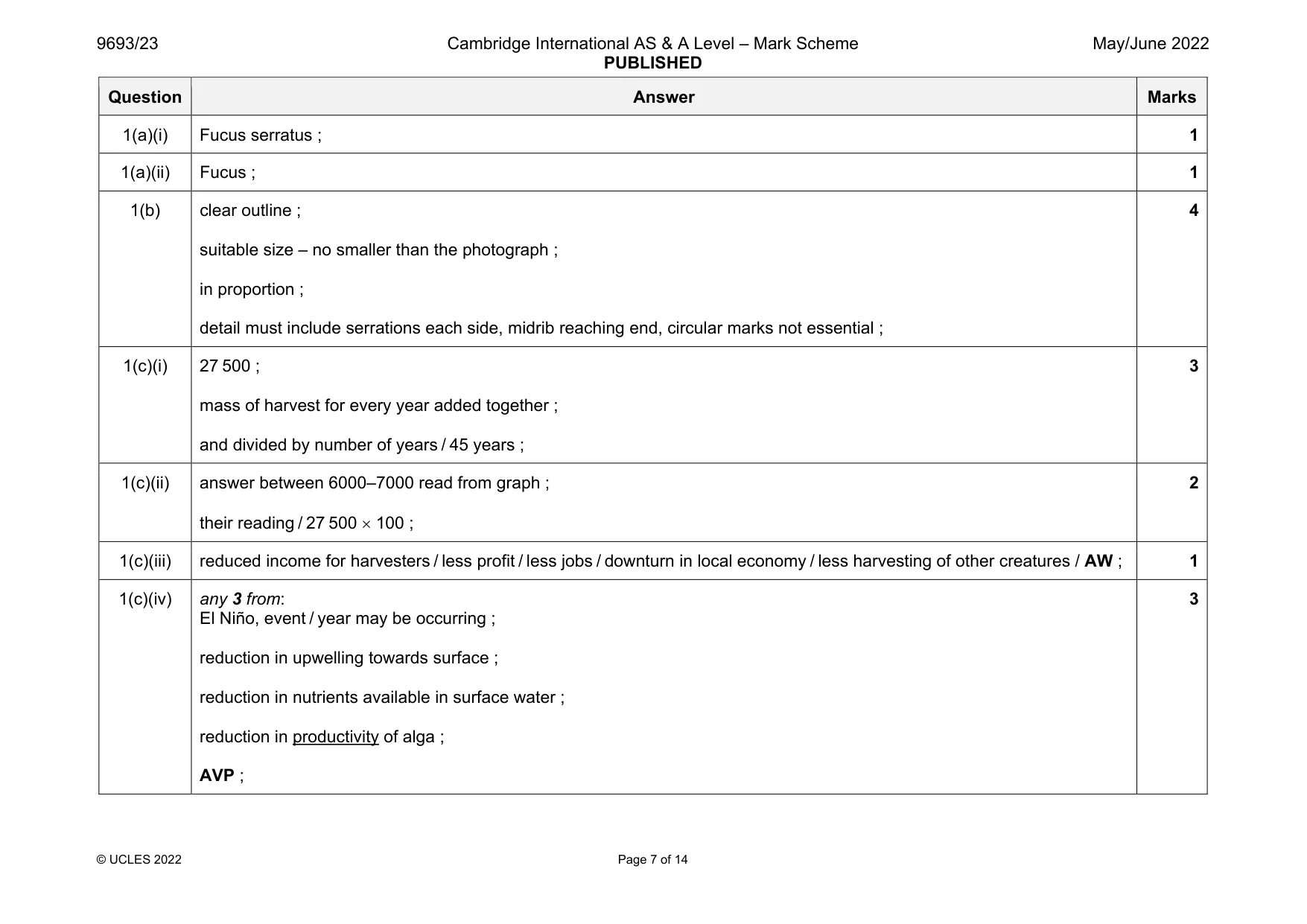
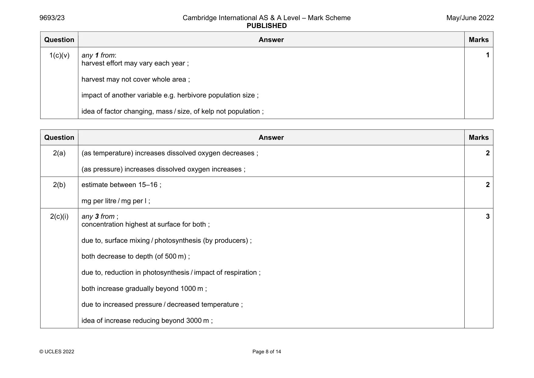
Mark scheme: 1(a)(i) Fucus serratus ; 1 1(a)(ii) Fucus ; 1 1(b) clear outline ; suitable size – no smaller than the photograph ; in proportion ; detail must include serrations each side, midrib reaching end, circular marks not essential ; 4 1(c)(i) 27 500 ; mass of harvest for every year added together ; and divided by number of years / 45 years ; 3 1(c)(ii) answer between 6000–7000 read from graph ; their reading / 27 500  100 ; 2 1(c)(iii) reduced income for harvesters / less profit / less jobs / downturn in local economy / less harvesting of other creatures / AW ; 1 1(c)(iv) any 3 from: El Niño, event / year may be occurring ; reduction in upwelling towards surface ; reduction in nutrients available in surface water ; reduction in productivity of alga ; AVP ; 3 Question Answer Marks 1(c)(v) any 1 from: harvest effort may vary each year ; harvest may not cover whole area ; impact of another variable e.g. herbivore population size ; idea of factor changing, mass / size, of kelp not population ; 1

More questions on Sustainable fisheries

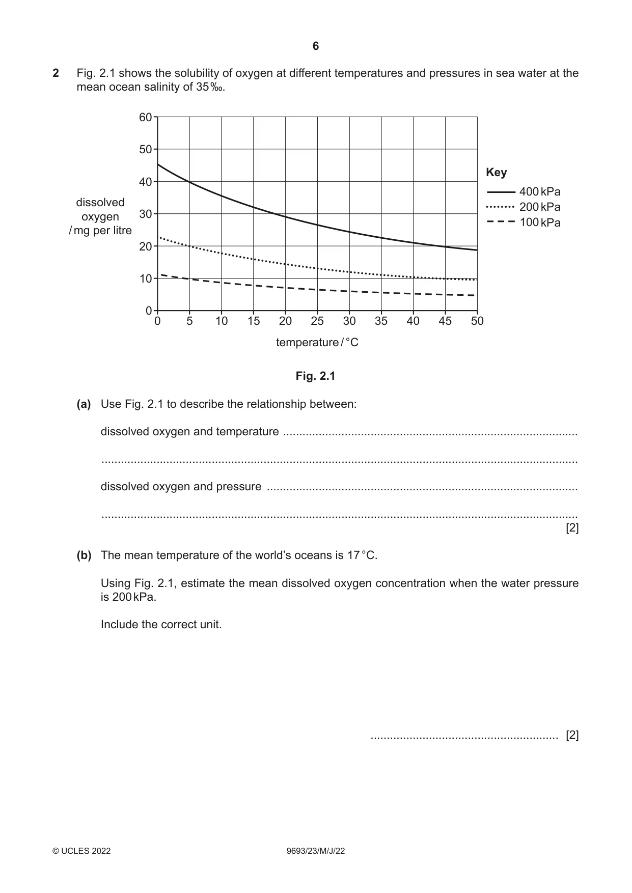
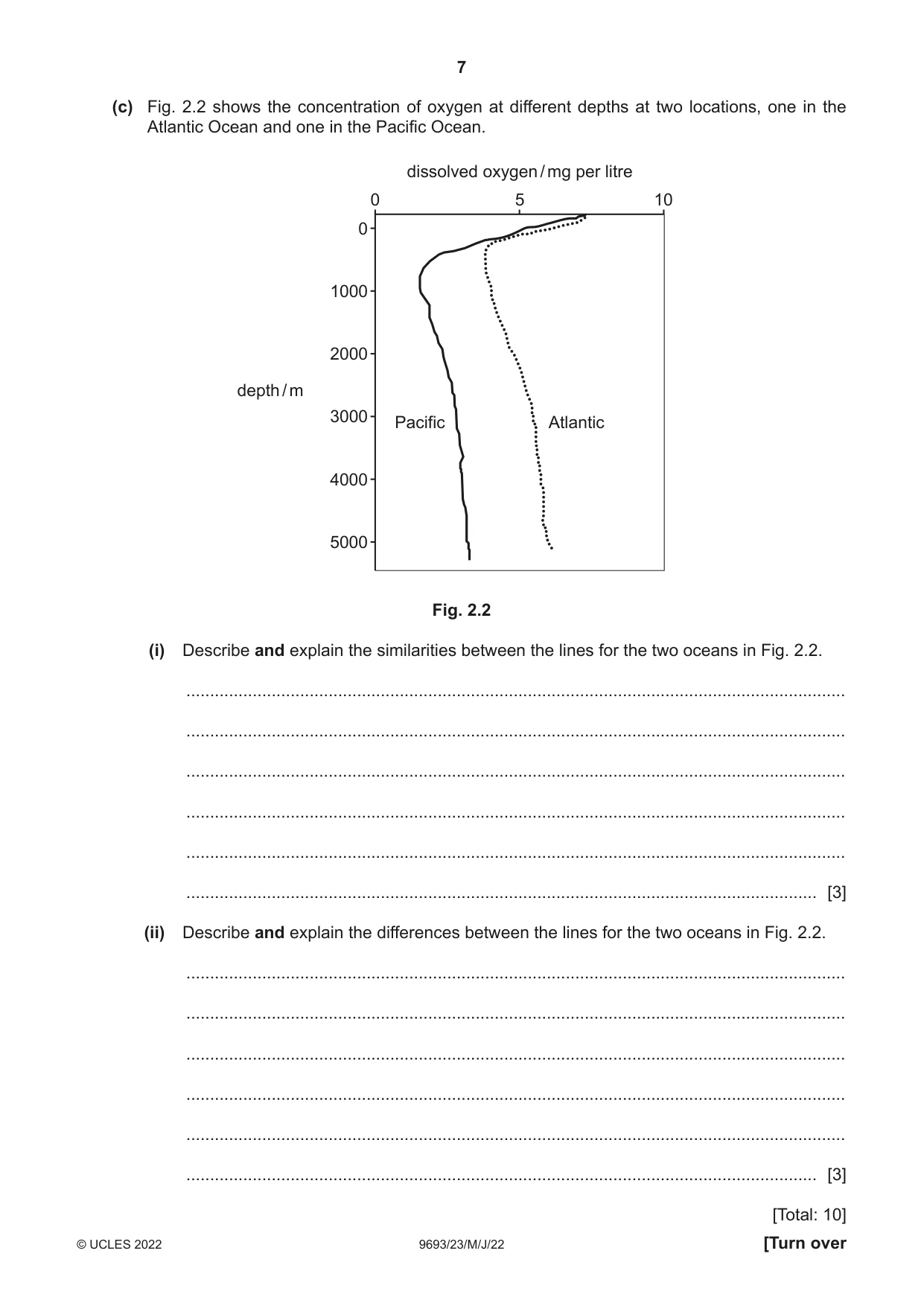
2 Fig. 2.1 shows the solubility of oxygen at different temperatures and pressures in sea water at the mean ocean salinity of 35 ‰. 60 50 Key 40 400 kPa dissolved 200 kPa oxygen 30 100 kPa / mg per litre 20 10 0 0 5 10 15 20 25 30 35 40 45 50 temperature / °C Fig. 2.1 (a) Use Fig. 2.1 to describe the relationship between: dissolved oxygen and temperature ........................................................................................... ................................................................................................................................................... dissolved oxygen and pressure ................................................................................................ ................................................................................................................................................... [2] (b) The mean temperature of the world’s oceans is 17 °C. Using Fig. 2.1, estimate the mean dissolved oxygen concentration when the water pressure is 200 kPa. Include the correct unit. .......................................................... [2] (c) Fig. 2.2 shows the concentration of oxygen at different depths at two locations, one in the Atlantic Ocean and one in the Pacific Ocean. dissolved oxygen / mg per litre 0 5 10 0 1000 2000 depth / m 3000 Pacific Atlantic 4000 5000 Fig. 2.2 (i) Describe and explain the similarities between the lines for the two oceans in Fig. 2.2. ........................................................................................................................................... ........................................................................................................................................... ........................................................................................................................................... ........................................................................................................................................... ........................................................................................................................................... ..................................................................................................................................... [3] (ii) Describe and explain the differences between the lines for the two oceans in Fig. 2.2. ........................................................................................................................................... ........................................................................................................................................... ........................................................................................................................................... ........................................................................................................................................... ........................................................................................................................................... ..................................................................................................................................... [3] [Total: 10]

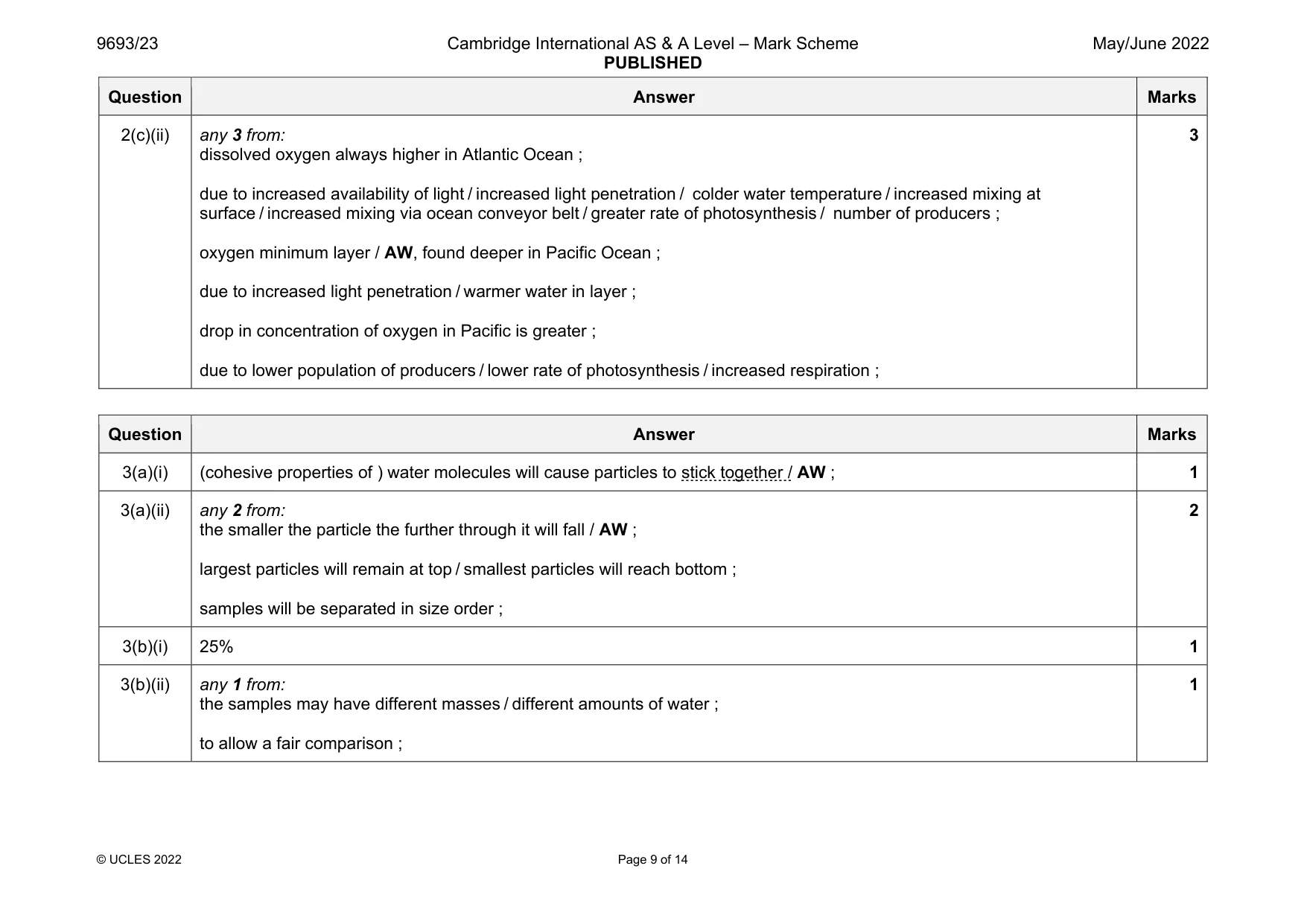
Mark scheme: 2(a) (as temperature) increases dissolved oxygen decreases ; (as pressure) increases dissolved oxygen increases ; 2(b) estimate between 15–16 ; mg per litre / mg per l ; 2 2(c)(i) any 3 from ; concentration highest at surface for both ; due to, surface mixing / photosynthesis (by producers) ; both decrease to depth (of 500 m) ; due to, reduction in photosynthesis / impact of respiration ; both increase gradually beyond 1000 m ; due to increased pressure / decreased temperature ; idea of increase reducing beyond 3000 m ; 3 Question Answer Marks 2(c)(ii) any 3 from: dissolved oxygen always higher in Atlantic Ocean ; due to increased availability of light / increased light penetration / colder water temperature / increased mixing at surface / increased mixing via ocean conveyor belt / greater rate of photosynthesis / number of producers ; oxygen minimum layer / AW, found deeper in Pacific Ocean ; due to increased light penetration / warmer water in layer ; drop in concentration of oxygen in Pacific is greater ; due to lower population of producers / lower rate of photosynthesis / increased respiration ; 3

More questions on The open ocean

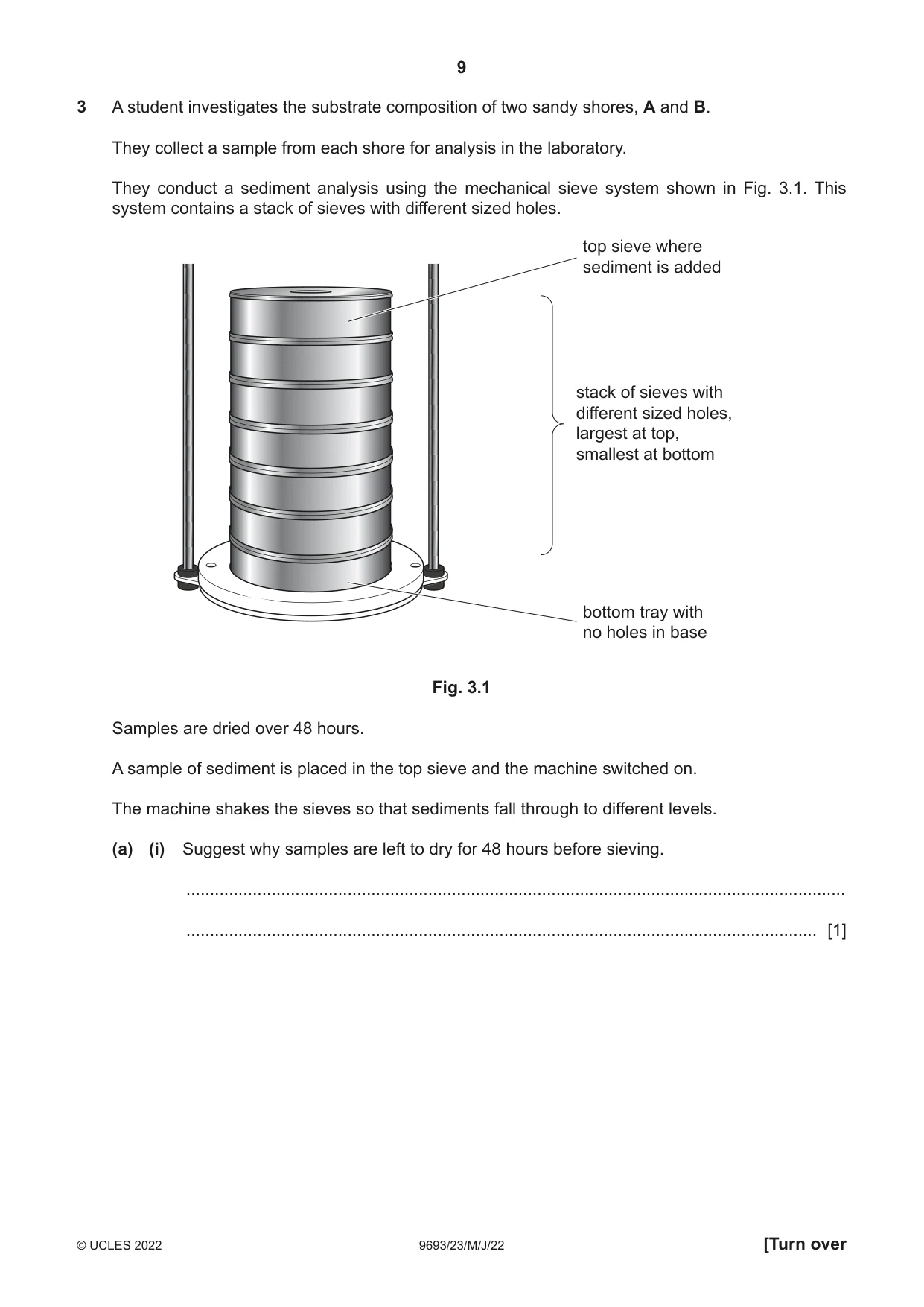
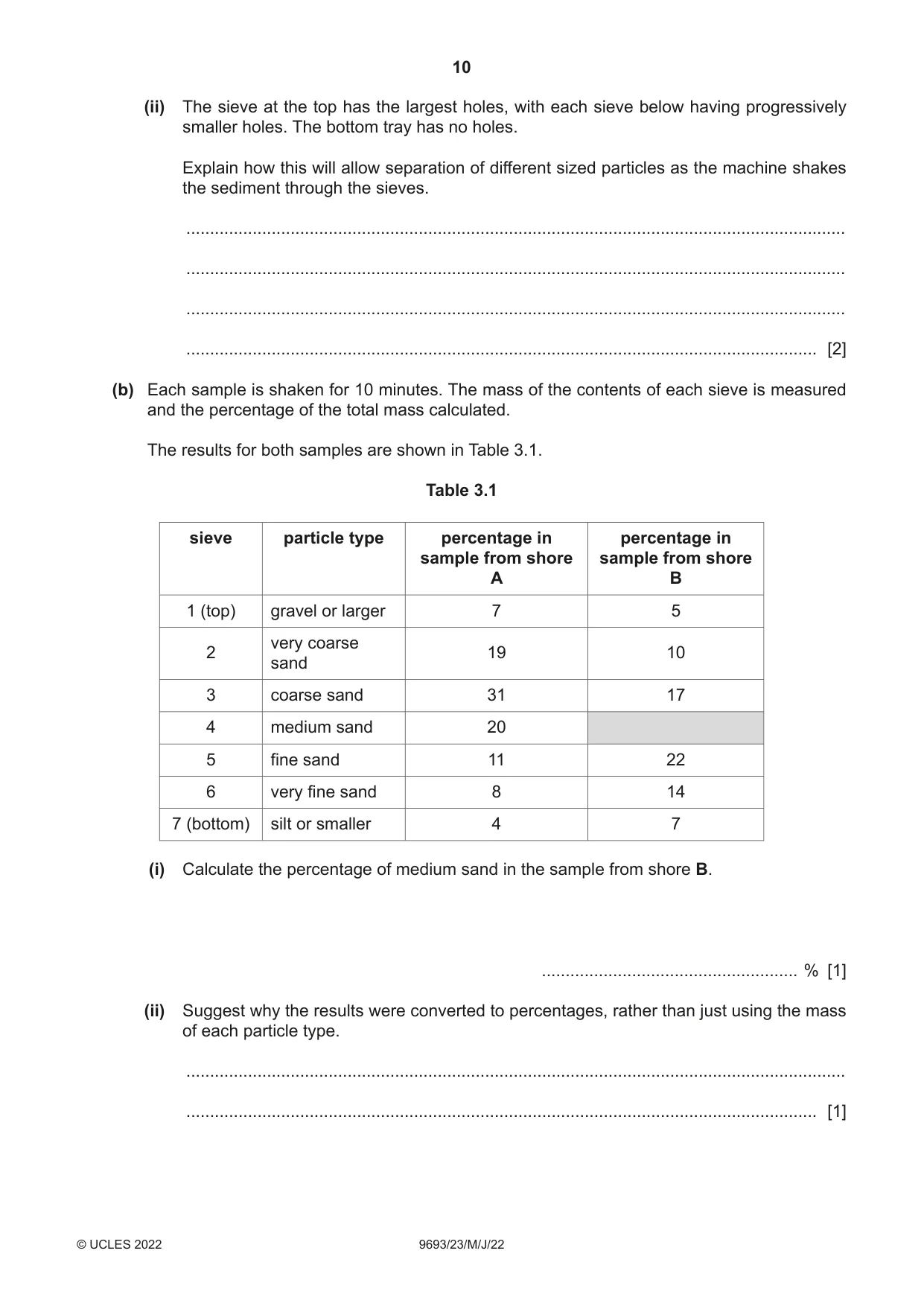
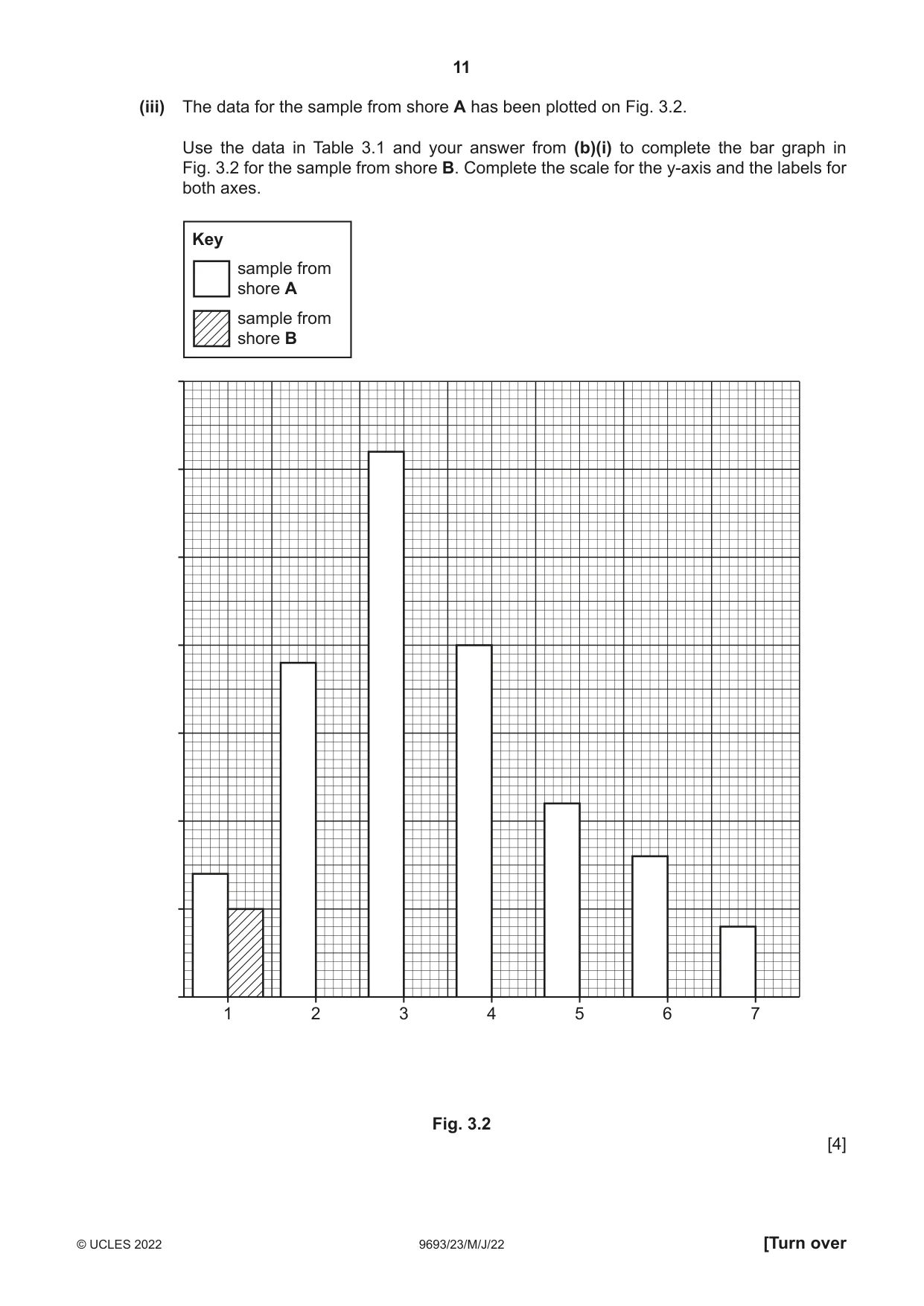
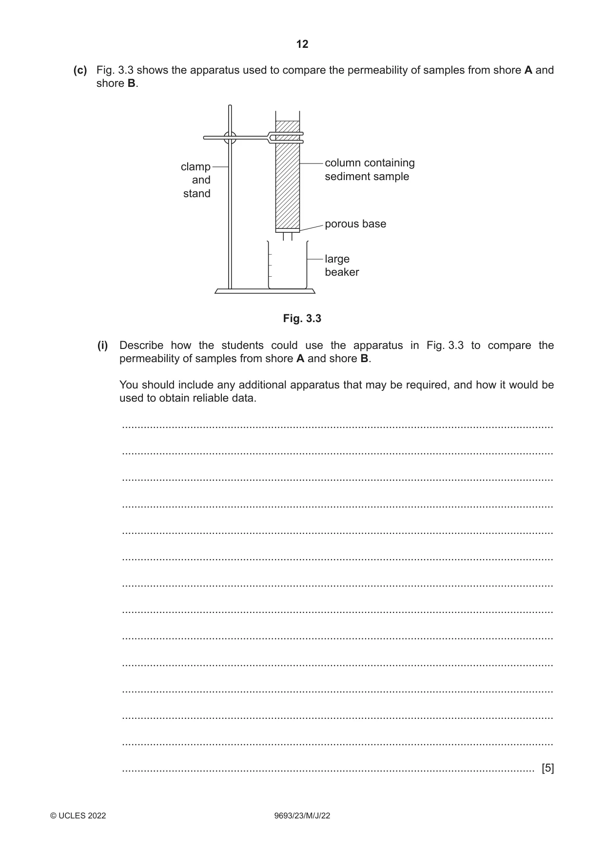
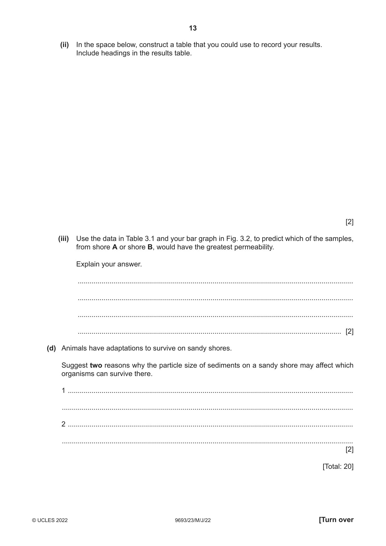
3 A student investigates the substrate composition of two sandy shores, A and B. They collect a sample from each shore for analysis in the laboratory. They conduct a sediment analysis using the mechanical sieve system shown in Fig. 3.1. This system contains a stack of sieves with different sized holes. top sieve where sediment is added stack of sieves with different sized holes, largest at top, smallest at bottom bottom tray with no holes in base Fig. 3.1 Samples are dried over 48 hours. A sample of sediment is placed in the top sieve and the machine switched on. The machine shakes the sieves so that sediments fall through to different levels. (a) (i) Suggest why samples are left to dry for 48 hours before sieving. ........................................................................................................................................... ..................................................................................................................................... [1] (ii) The sieve at the top has the largest holes, with each sieve below having progressively smaller holes. The bottom tray has no holes. Explain how this will allow separation of different sized particles as the machine shakes the sediment through the sieves. ........................................................................................................................................... ........................................................................................................................................... ........................................................................................................................................... ..................................................................................................................................... [2] (b) Each sample is shaken for 10 minutes. The mass of the contents of each sieve is measured and the percentage of the total mass calculated. The results for both samples are shown in Table 3.1. Table 3.1 sieve particle type percentage in percentage in sample from shore sample from shore A B 1 (top) gravel or larger 7 5 very coarse 2 19 10 sand 3 coarse sand 31 17 4 medium sand 20 5 fine sand 11 22 6 very fine sand 8 14 7 (bottom) silt or smaller 4 7 (i) Calculate the percentage of medium sand in the sample from shore B. ...................................................... % [1] (ii) Suggest why the results were converted to percentages, rather than just using the mass of each particle type. ........................................................................................................................................... ..................................................................................................................................... [1] (iii) The data for the sample from shore A has been plotted on Fig. 3.2. Use the data in Table 3.1 and your answer from (b)(i) to complete the bar graph in Fig. 3.2 for the sample from shore B. Complete the scale for the y-axis and the labels for both axes. Key sample from shore A sample from shore B 1 2 3 4 5 6 7 Fig. 3.2 [4] (c) Fig. 3.3 shows the apparatus used to compare the permeability of samples from shore A and shore B. column containing clamp sediment sample and stand porous base large beaker Fig. 3.3 (i) Describe how the students could use the apparatus in Fig. 3.3 to compare the permeability of samples from shore A and shore B. You should include any additional apparatus that may be required, and how it would be used to obtain reliable data. ........................................................................................................................................... ........................................................................................................................................... ........................................................................................................................................... ........................................................................................................................................... ........................................................................................................................................... ........................................................................................................................................... ........................................................................................................................................... ........................................................................................................................................... ........................................................................................................................................... ........................................................................................................................................... ........................................................................................................................................... ........................................................................................................................................... ........................................................................................................................................... ..................................................................................................................................... [5] (ii) In the space below, construct a table that you could use to record your results. Include headings in the results table. [2] (iii) Use the data in Table 3.1 and your bar graph in Fig. 3.2, to predict which of the samples, from shore A or shore B, would have the greatest permeability. Explain your answer. ........................................................................................................................................... ........................................................................................................................................... ........................................................................................................................................... ..................................................................................................................................... [2] (d) Animals have adaptations to survive on sandy shores. Suggest two reasons why the particle size of sediments on a sandy shore may affect which organisms can survive there. 1 ................................................................................................................................................ ................................................................................................................................................... 2 ................................................................................................................................................ ................................................................................................................................................... [2] [Total: 20]

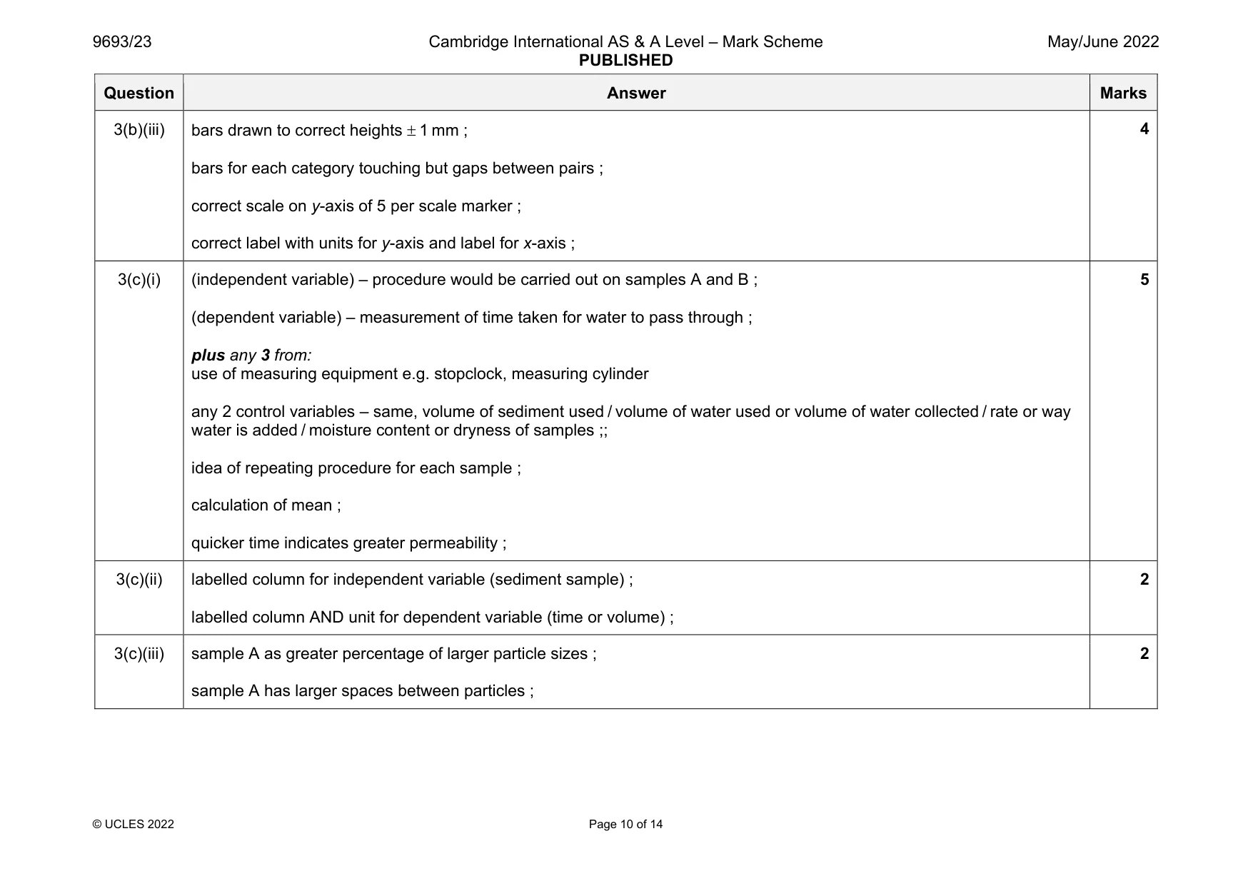
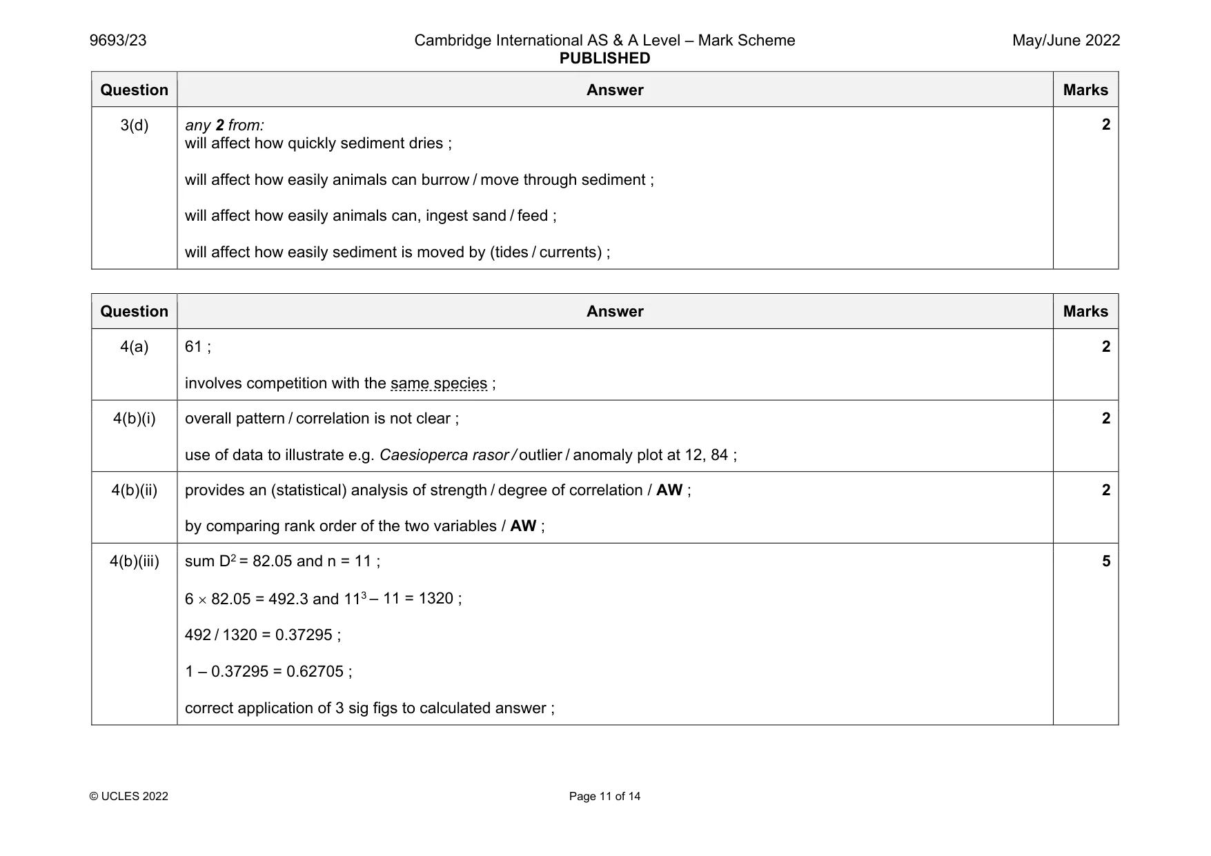
Mark scheme: 3(a)(i) (cohesive properties of ) water molecules will cause particles to stick together / AW ; 1 3(a)(ii) any 2 from: the smaller the particle the further through it will fall / AW ; largest particles will remain at top / smallest particles will reach bottom ; samples will be separated in size order ; 2 3(b)(i) 25% 1 3(b)(ii) any 1 from: the samples may have different masses / different amounts of water ; to allow a fair comparison ; 1 Question Answer Marks 3(b)(iii) bars drawn to correct heights  1 mm ; bars for each category touching but gaps between pairs ; correct scale on y-axis of 5 per scale marker ; correct label with units for y-axis and label for x-axis ; 4 3(c)(i) (independent variable) – procedure would be carried out on samples A and B ; (dependent variable) – measurement of time taken for water to pass through ; plus any 3 from: use of measuring equipment e.g. stopclock, measuring cylinder any 2 control variables – same, volume of sediment used / volume of water used or volume of water collected / rate or way water is added / moisture content or dryness of samples ;; idea of repeating procedure for each sample ; calculation of mean ; quicker time indicates greater permeability ; 5 3(c)(ii) labelled column for independent variable (sediment sample) ; labelled column AND unit for dependent variable (time or volume) ; 2 3(c)(iii) sample A as greater percentage of larger particle sizes ; sample A has larger spaces between particles ; 2 Question Answer Marks 3(d) any 2 from: will affect how quickly sediment dries ; will affect how easily animals can burrow / move through sediment ; will affect how easily animals can, ingest sand / feed ; will affect how easily sediment is moved by (tides / currents) ; 2

More questions on The sandy shore

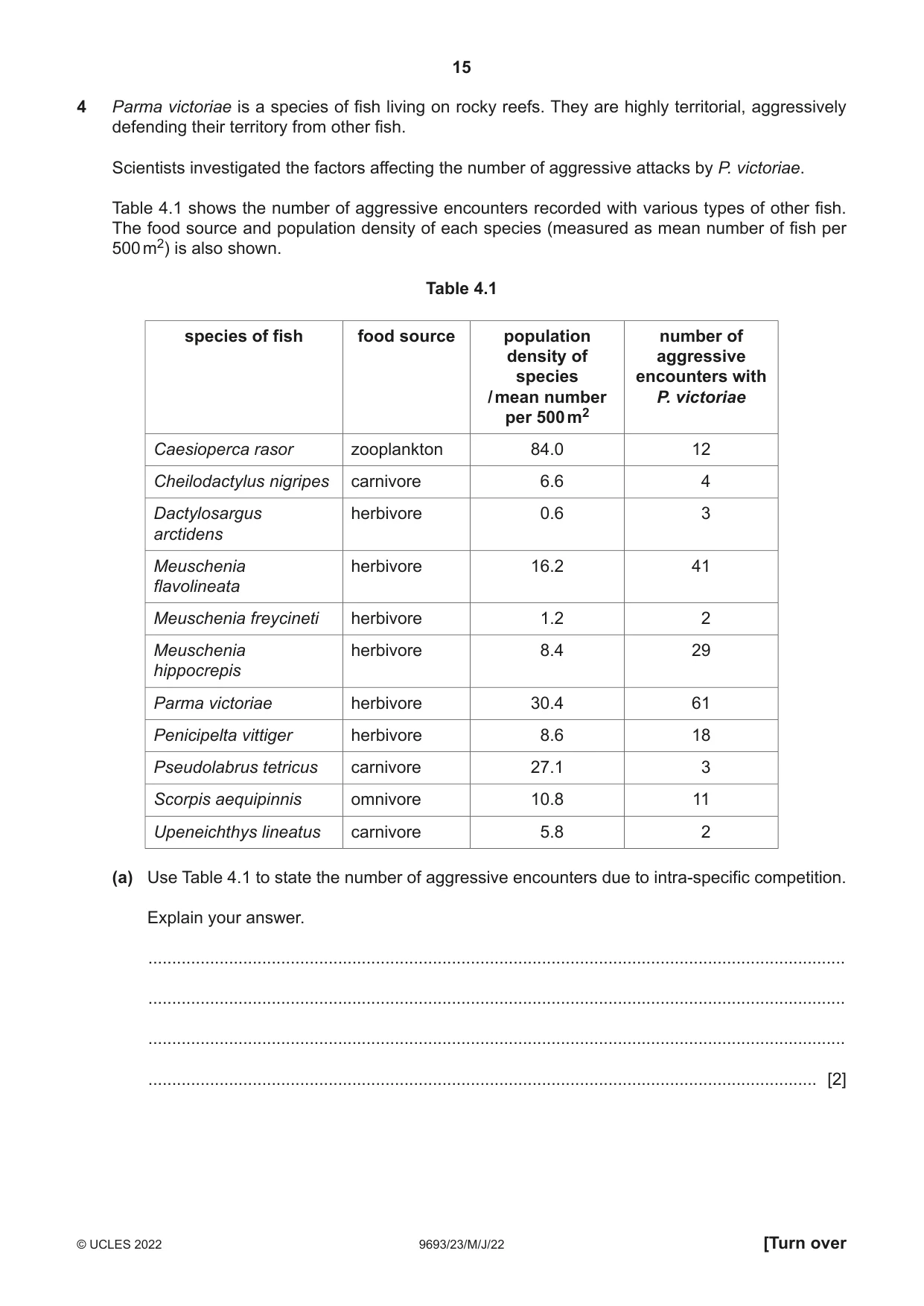
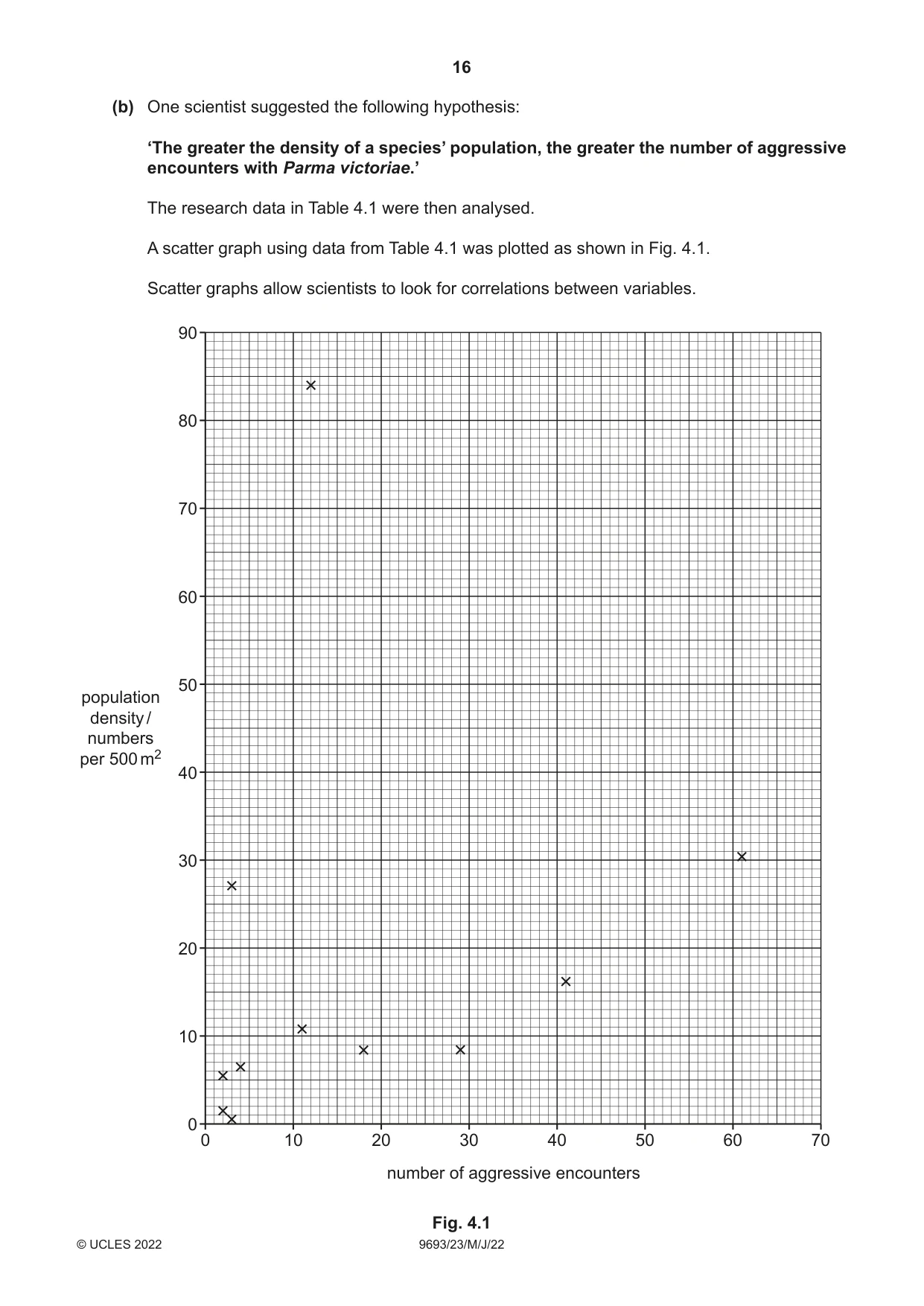
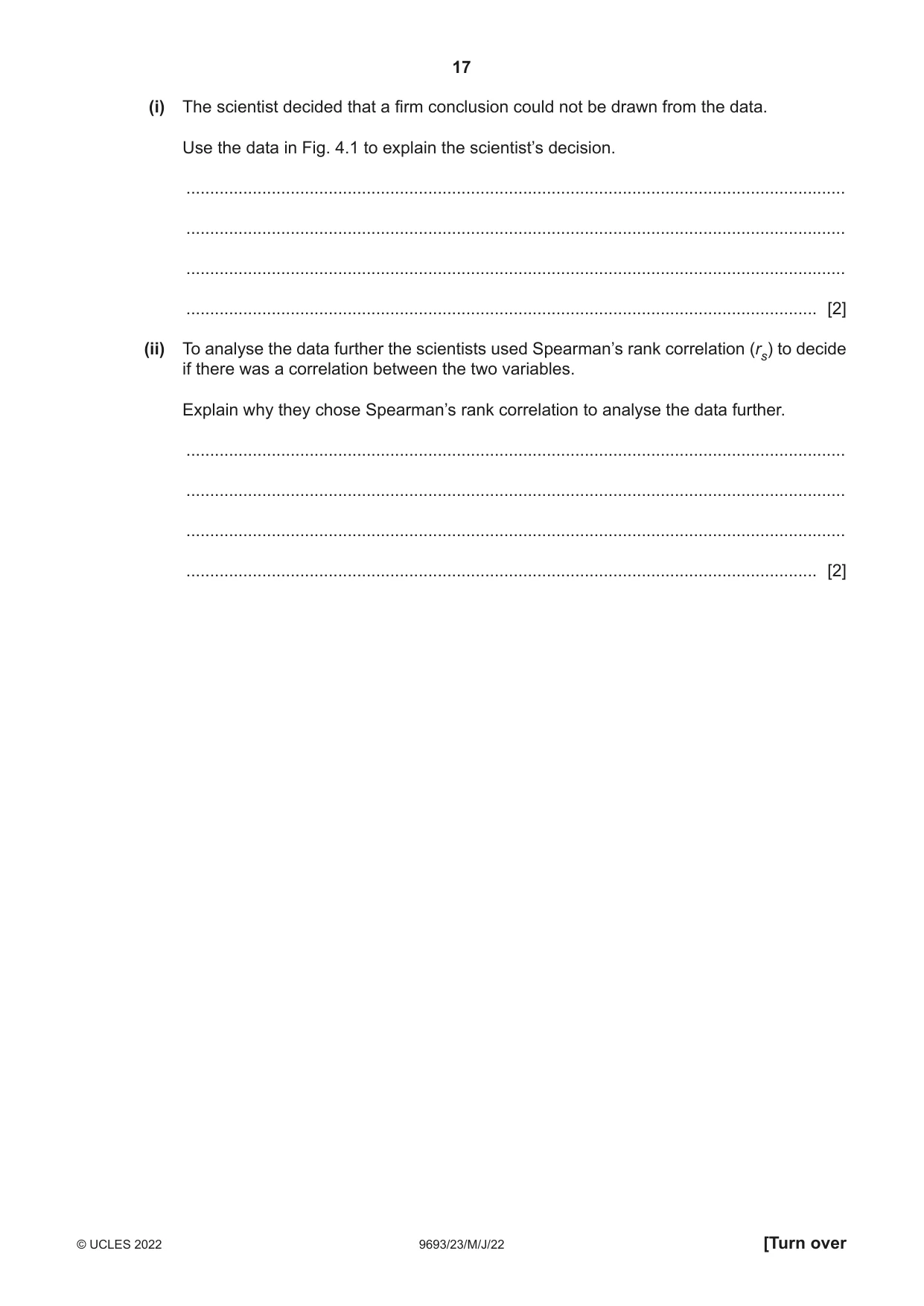
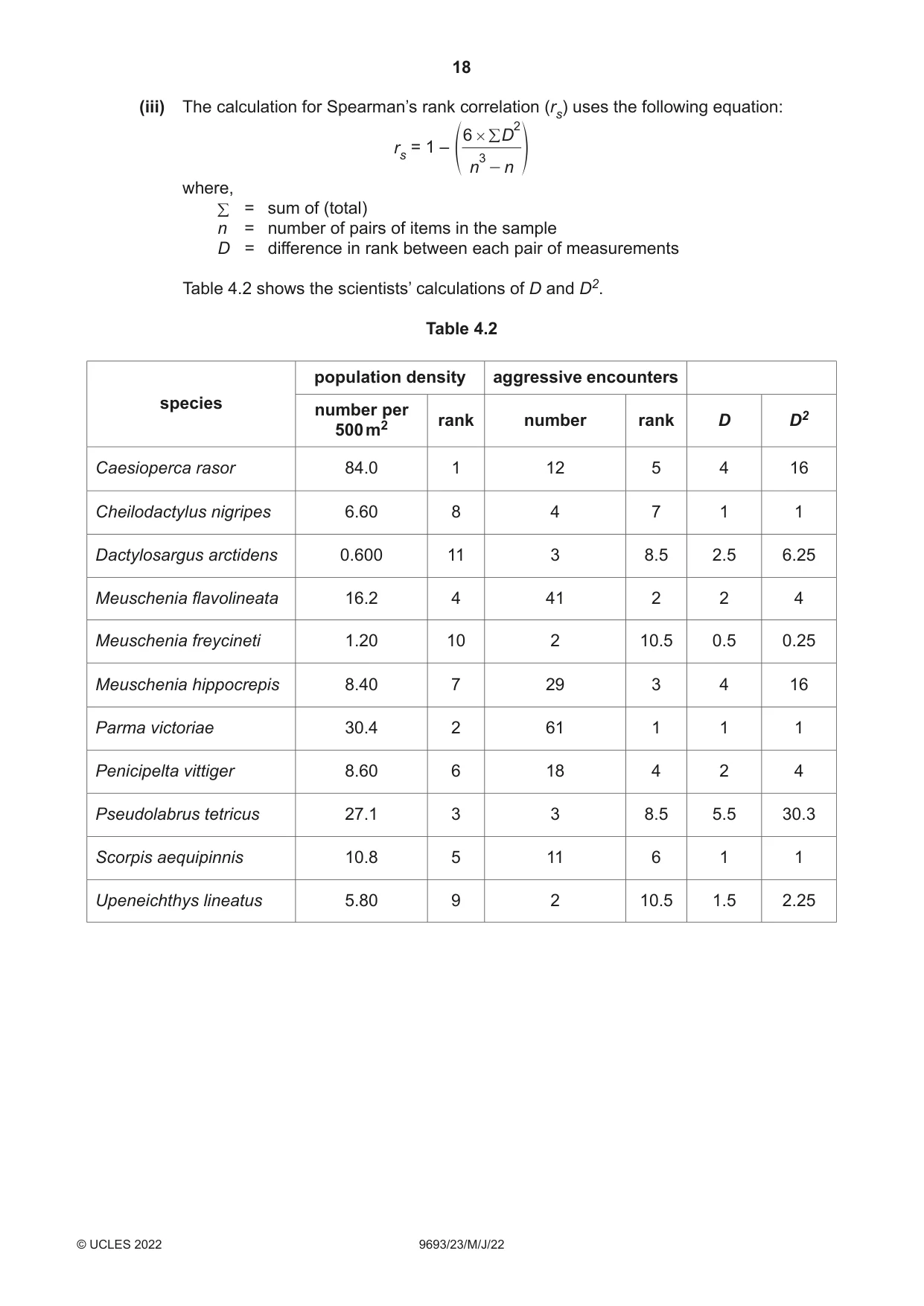
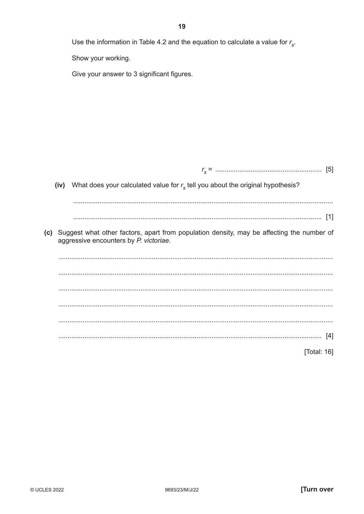
4 Parma victoriae is a species of fish living on rocky reefs. They are highly territorial, aggressively defending their territory from other fish. Scientists investigated the factors affecting the number of aggressive attacks by P. victoriae. Table 4.1 shows the number of aggressive encounters recorded with various types of other fish. The food source and population density of each species (measured as mean number of fish per 500 m2) is also shown. Table 4.1 species of fish food source population number of density of aggressive species encounters with / mean number P. victoriae per 500 m2 Caesioperca rasor zooplankton 84.0 12 Cheilodactylus nigripes carnivore 6.6 4 Dactylosargus herbivore 0.6 3 arctidens Meuschenia herbivore 16.2 41 flavolineata Meuschenia freycineti herbivore 1.2 2 Meuschenia herbivore 8.4 29 hippocrepis Parma victoriae herbivore 30.4 61 Penicipelta vittiger herbivore 8.6 18 Pseudolabrus tetricus carnivore 27.1 3 Scorpis aequipinnis omnivore 10.8 11 Upeneichthys lineatus carnivore 5.8 2 (a) Use Table 4.1 to state the number of aggressive encounters due to intra-specific competition. Explain your answer. ................................................................................................................................................... ................................................................................................................................................... ................................................................................................................................................... ............................................................................................................................................. [2] (i) The scientist decided that a firm conclusion could not be drawn from the data. Use the data in Fig. 4.1 to explain the scientist’s decision. ........................................................................................................................................... ........................................................................................................................................... ........................................................................................................................................... ..................................................................................................................................... [2] (ii) To analyse the data further the scientists used Spearman’s rank correlation (rs) to decide if there was a correlation between the two variables. Explain why they chose Spearman’s rank correlation to analyse the data further. ........................................................................................................................................... ........................................................................................................................................... ........................................................................................................................................... ..................................................................................................................................... [2] (iii) The calculation for Spearman’s rank correlation (rs) uses the following equation: 2 6 # / D rs = 1 – 3 f n - n p where, / = sum of (total) n = number of pairs of items in the sample D = difference in rank between each pair of measurements Table 4.2 shows the scientists’ calculations of D and D2. Table 4.2 population density aggressive encounters species number per rank number rank D D2 500 m2 Caesioperca rasor 84.0 1 12 5 4 16 Cheilodactylus nigripes 6.60 8 4 7 1 1 Dactylosargus arctidens 0.600 11 3 8.5 2.5 6.25 Meuschenia flavolineata 16.2 4 41 2 2 4 Meuschenia freycineti 1.20 10 2 10.5 0.5 0.25 Meuschenia hippocrepis 8.40 7 29 3 4 16 Parma victoriae 30.4 2 61 1 1 1 Penicipelta vittiger 8.60 6 18 4 2 4 Pseudolabrus tetricus 27.1 3 3 8.5 5.5 30.3 Scorpis aequipinnis 10.8 5 11 6 1 1 Upeneichthys lineatus 5.80 9 2 10.5 1.5 2.25 Use the information in Table 4.2 and the equation to calculate a value for rs. Show your working. Give your answer to 3 significant figures. rs = ......................................................... [5] (iv) What does your calculated value for rs tell you about the original hypothesis? ........................................................................................................................................... ..................................................................................................................................... [1] (c) Suggest what other factors, apart from population density, may be affecting the number of aggressive encounters by P. victoriae. ................................................................................................................................................... ................................................................................................................................................... ................................................................................................................................................... ................................................................................................................................................... ................................................................................................................................................... ............................................................................................................................................. [4] [Total: 16]

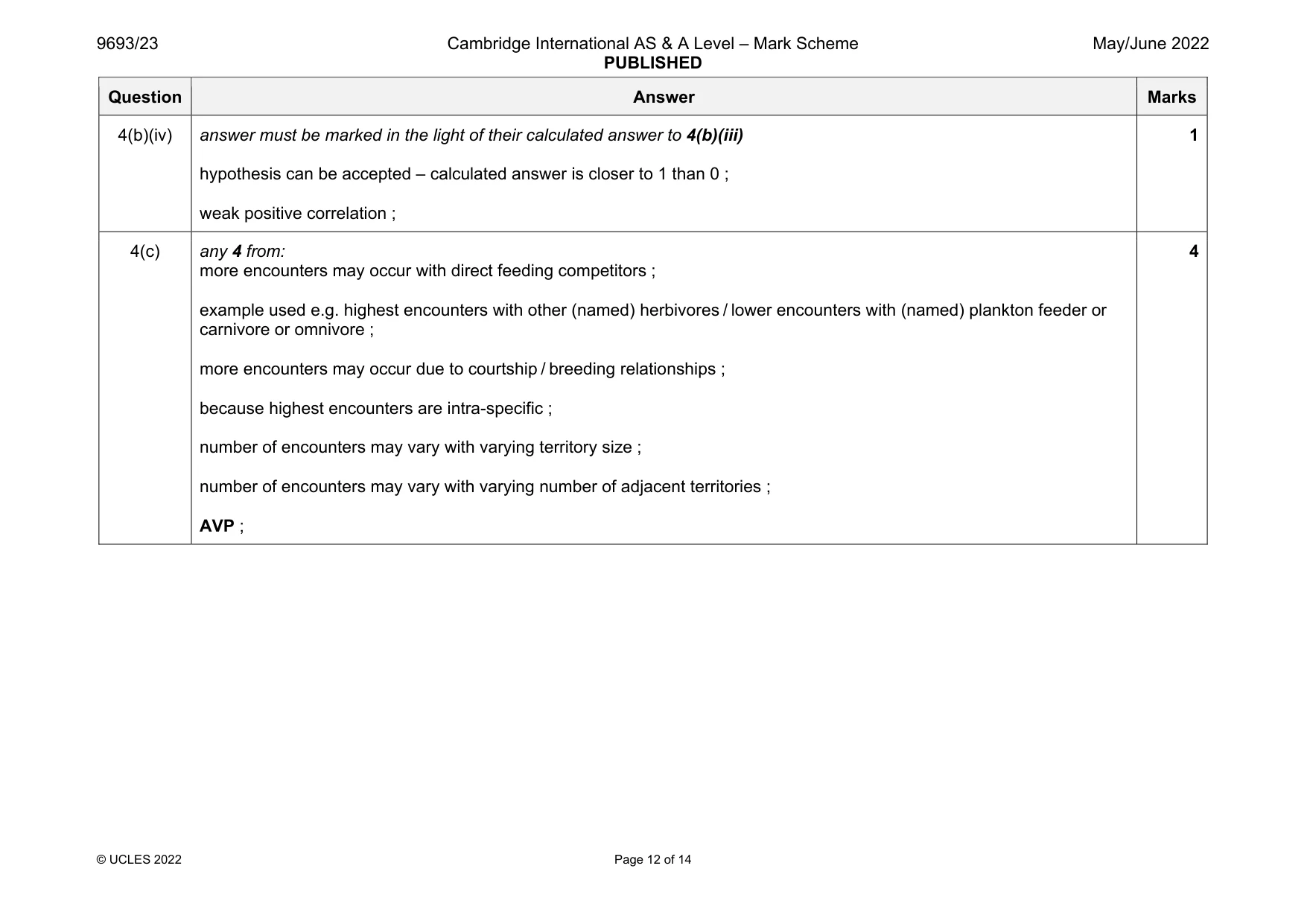
Mark scheme: 4(a) 61 ; involves competition with the same species ; 2 4(b)(i) overall pattern / correlation is not clear ; use of data to illustrate e.g. Caesioperca rasor / outlier / anomaly plot at 12, 84 ; 2 4(b)(ii) provides an (statistical) analysis of strength / degree of correlation / AW ; by comparing rank order of the two variables / AW ; 2 4(b)(iii) sum D2 = 82.05 and n = 11 ; 6  82.05 = 492.3 and 113 – 11 = 1320 ; 492 / 1320 = 0.37295 ; 1 – 0.37295 = 0.62705 ; correct application of 3 sig figs to calculated answer ; 5 Question Answer Marks 4(b)(iv) answer must be marked in the light of their calculated answer to 4(b)(iii) hypothesis can be accepted – calculated answer is closer to 1 than 0 ; weak positive correlation ; 1 4(c) any 4 from: more encounters may occur with direct feeding competitors ; example used e.g. highest encounters with other (named) herbivores / lower encounters with (named) plankton feeder or carnivore or omnivore ; more encounters may occur due to courtship / breeding relationships ; because highest encounters are intra-specific ; number of encounters may vary with varying territory size ; number of encounters may vary with varying number of adjacent territories ; AVP ; 4

More questions on Populations and sampling techniques

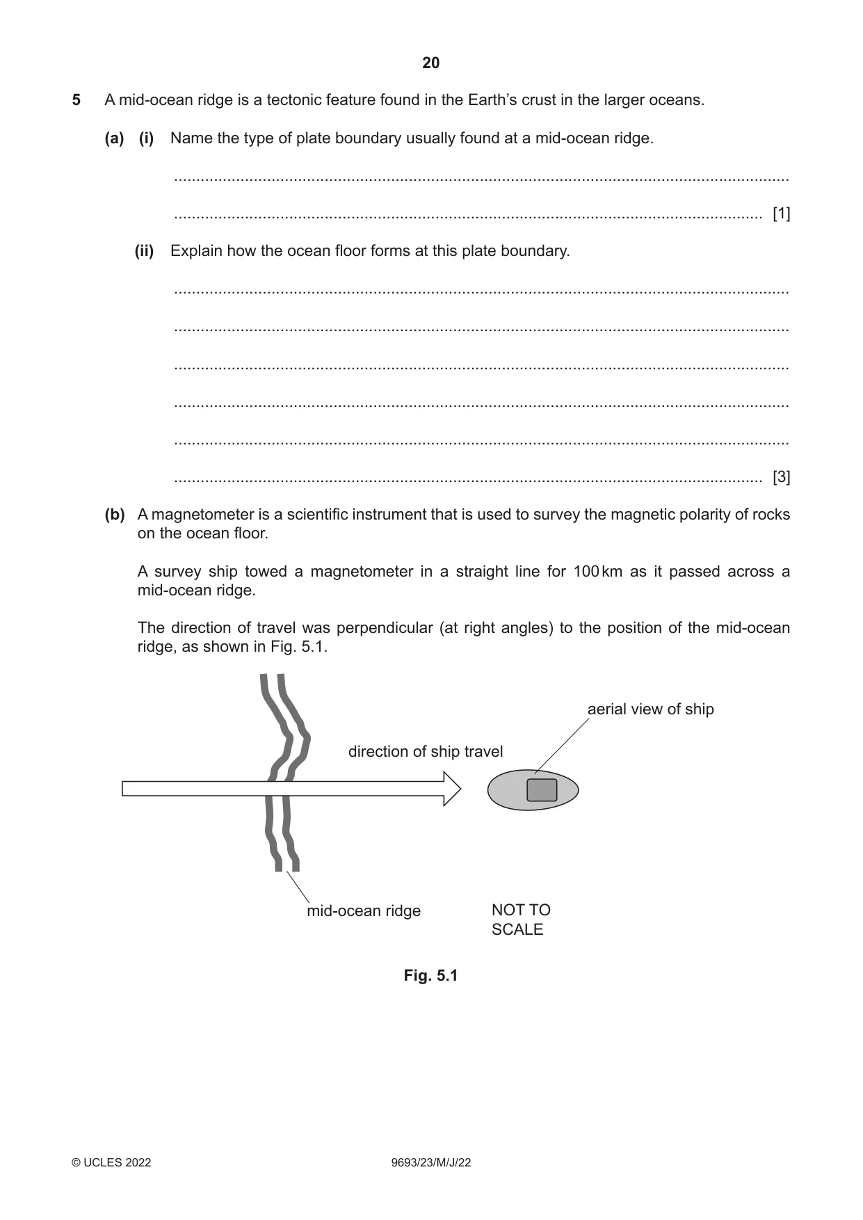
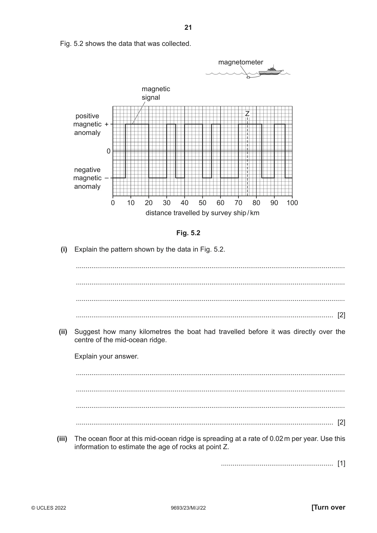
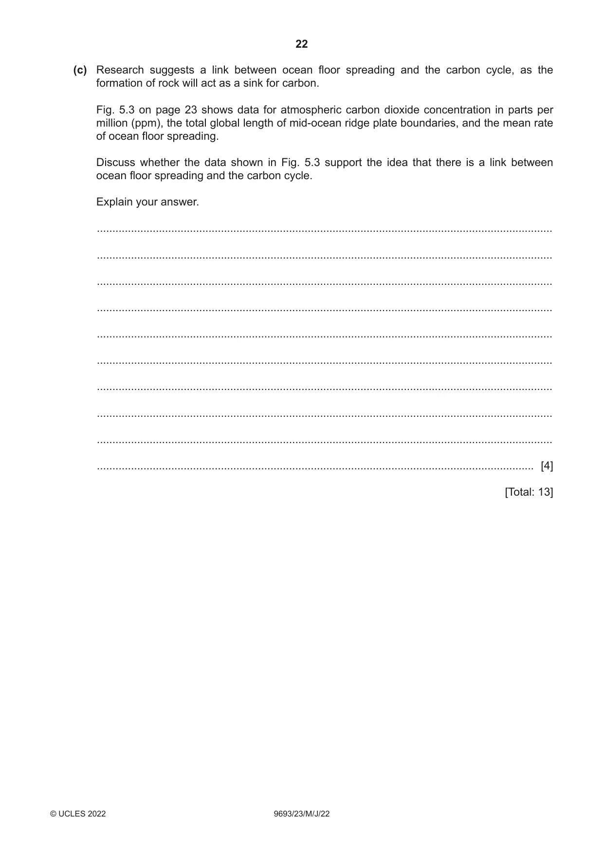
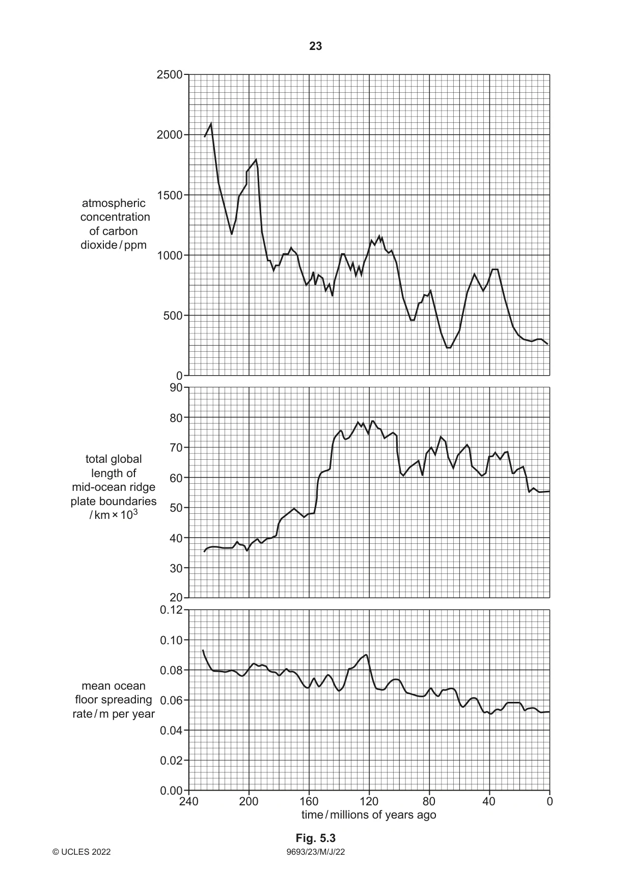
5 A mid-ocean ridge is a tectonic feature found in the Earth’s crust in the larger oceans. (a) (i) Name the type of plate boundary usually found at a mid-ocean ridge. ........................................................................................................................................... ..................................................................................................................................... [1] (ii) Explain how the ocean floor forms at this plate boundary. ........................................................................................................................................... ........................................................................................................................................... ........................................................................................................................................... ........................................................................................................................................... ........................................................................................................................................... ..................................................................................................................................... [3] (b) A magnetometer is a scientific instrument that is used to survey the magnetic polarity of rocks on the ocean floor. A survey ship towed a magnetometer in a straight line for 100 km as it passed across a mid-ocean ridge. The direction of travel was perpendicular (at right angles) to the position of the mid-ocean ridge, as shown in Fig. 5.1. aerial view of ship direction of ship travel mid-ocean ridge NOT TO SCALE Fig. 5.1 Fig. 5.2 shows the data that was collected. magnetometer magnetic signal Z positive magnetic + anomaly 0 negative magnetic – anomaly 0 10 20 30 40 50 60 70 80 90 100 distance travelled by survey ship / km Fig. 5.2 (i) Explain the pattern shown by the data in Fig. 5.2. ........................................................................................................................................... ........................................................................................................................................... ........................................................................................................................................... ..................................................................................................................................... [2] (ii) Suggest how many kilometres the boat had travelled before it was directly over the centre of the mid-ocean ridge. Explain your answer. ........................................................................................................................................... ........................................................................................................................................... ........................................................................................................................................... ..................................................................................................................................... [2] (iii) The ocean floor at this mid-ocean ridge is spreading at a rate of 0.02 m per year. Use this information to estimate the age of rocks at point Z. .......................................................... [1] (c) Research suggests a link between ocean floor spreading and the carbon cycle, as the formation of rock will act as a sink for carbon. Fig. 5.3 on page 23 shows data for atmospheric carbon dioxide concentration in parts per million (ppm), the total global length of mid-ocean ridge plate boundaries, and the mean rate of ocean floor spreading. Discuss whether the data shown in Fig. 5.3 support the idea that there is a link between ocean floor spreading and the carbon cycle. Explain your answer. ................................................................................................................................................... ................................................................................................................................................... ................................................................................................................................................... ................................................................................................................................................... ................................................................................................................................................... ................................................................................................................................................... ................................................................................................................................................... ................................................................................................................................................... ................................................................................................................................................... ............................................................................................................................................. [4] [Total: 13]

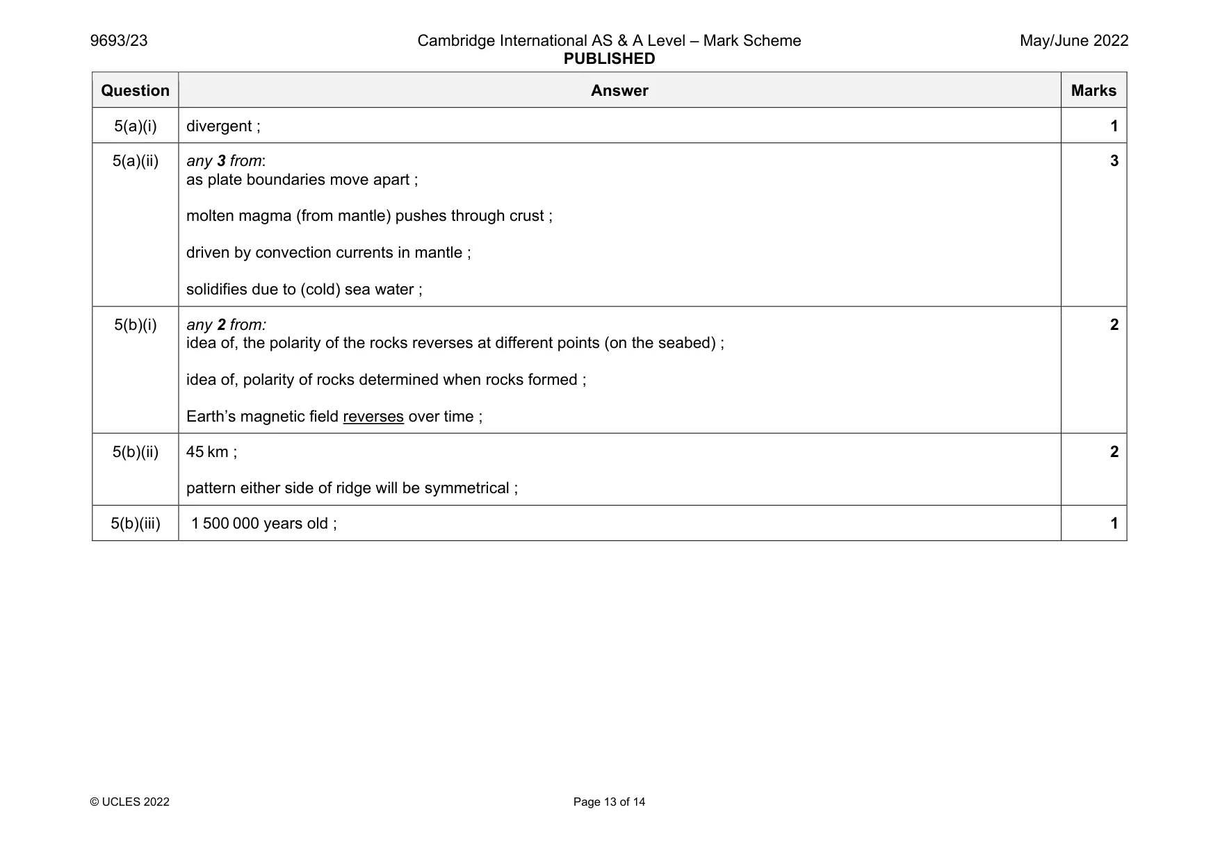
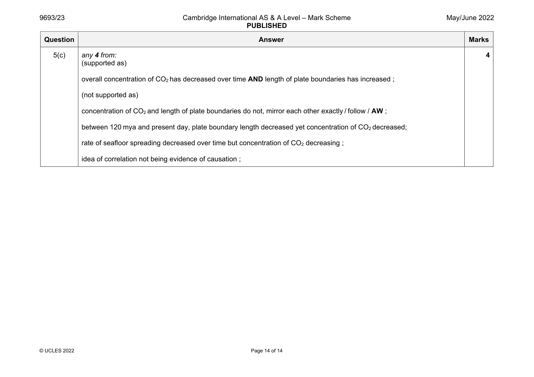
Mark scheme: 5(a)(i) divergent ; 1 5(a)(ii) any 3 from: as plate boundaries move apart ; molten magma (from mantle) pushes through crust ; driven by convection currents in mantle ; solidifies due to (cold) sea water ; 3 5(b)(i) any 2 from: idea of, the polarity of the rocks reverses at different points (on the seabed) ; idea of, polarity of rocks determined when rocks formed ; Earth’s magnetic field reverses over time ; 2 5(b)(ii) 45 km ; pattern either side of ridge will be symmetrical ; 2 5(b)(iii) 1 500 000 years old ; 1 Question Answer Marks 5(c) any 4 from: (supported as) overall concentration of CO2 has decreased over time AND length of plate boundaries has increased ; (not supported as) concentration of CO2 and length of plate boundaries do not, mirror each other exactly / follow / AW ; between 120 mya and present day, plate boundary length decreased yet concentration of CO2 decreased; rate of seafloor spreading decreased over time but concentration of CO2 decreasing ; idea of correlation not being evidence of causation ; 4

More questions on Tectonic processes