Cambridge A Level Marine Science 9693 — 2024 May/June Paper 4 · Variant 3

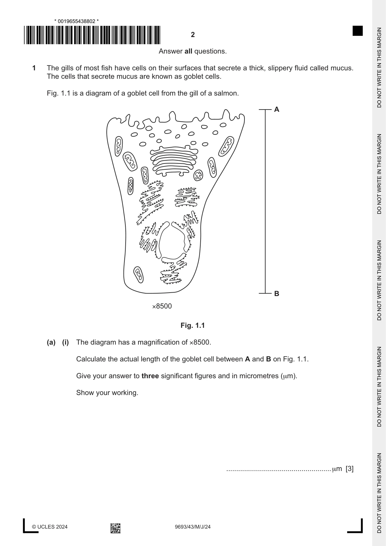
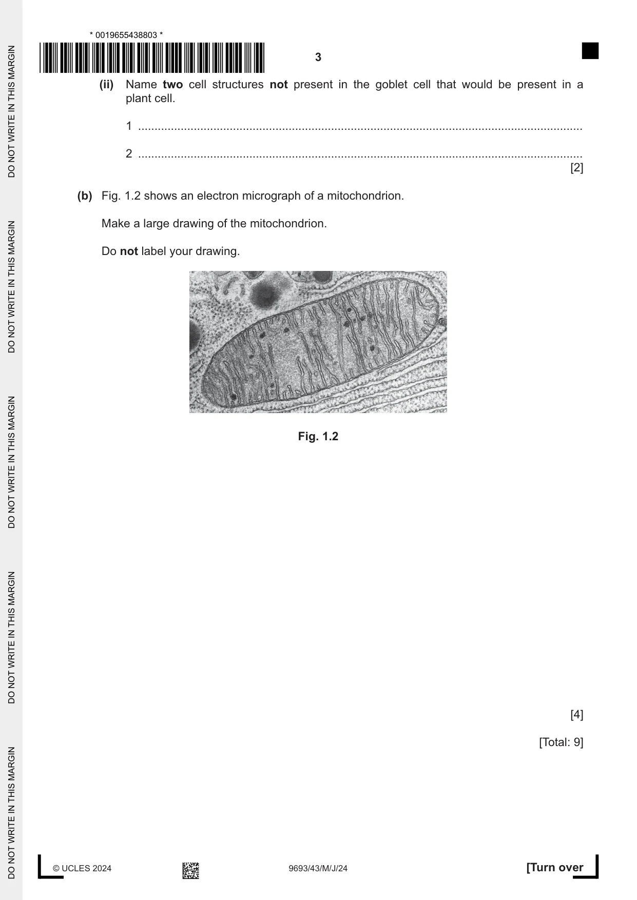
1 The gills of most fish have cells on their surfaces that secrete a thick, slippery fluid called mucus. The cells that secrete mucus are known as goblet cells. Fig. 1.1 is a diagram of a goblet cell from the gill of a salmon. A B ×8500 Fig. 1.1 (a) (i) The diagram has a magnification of ×8500. Calculate the actual length of the goblet cell between A and B on Fig. 1.1. Give your answer to three significant figures and in micrometres (μm). Show your working. ..................................................... μm [3] (ii) Name two cell structures not present in the goblet cell that would be present in a plant cell. 1 ........................................................................................................................................ 2 ........................................................................................................................................ [2] (b) Fig. 1.2 shows an electron micrograph of a mitochondrion. Make a large drawing of the mitochondrion. Do not label your drawing. Fig. 1.2 [4] [Total: 9]

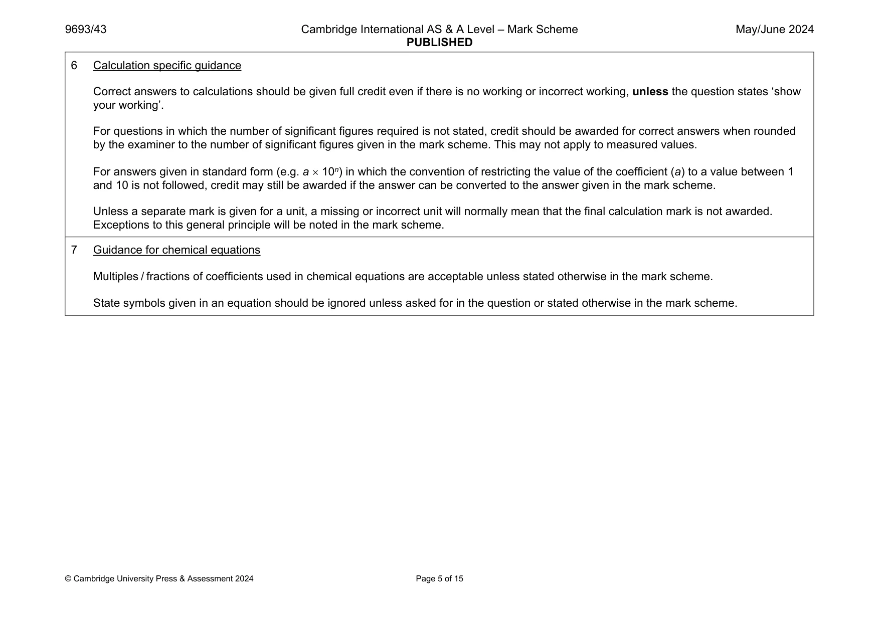
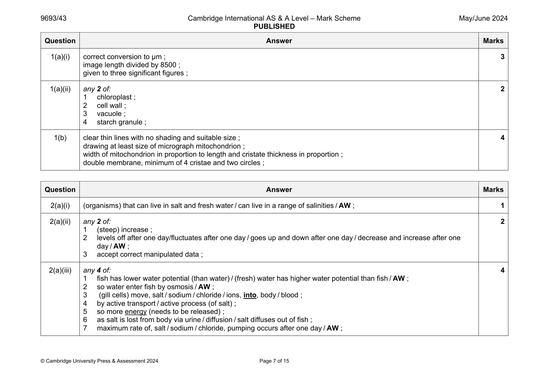
Mark scheme: 1(a)(i) correct conversion to µm ; image length divided by 8500 ; given to three significant figures ; 3 1(a)(ii) any 2 of: 1 chloroplast ; 2 cell wall ; 3 vacuole ; 4 starch granule ; 2 1(b) clear thin lines with no shading and suitable size ; drawing at least size of micrograph mitochondrion ; width of mitochondrion in proportion to length and cristate thickness in proportion ; double membrane, minimum of 4 cristae and two circles ; 4

More questions on General cell structure

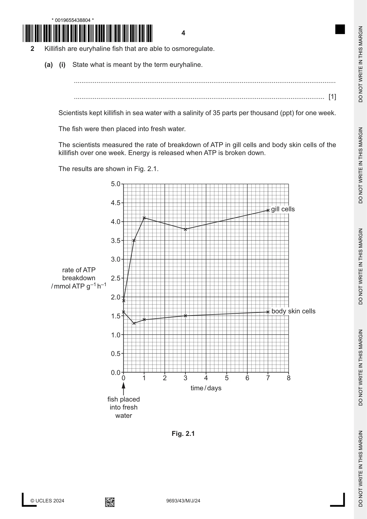
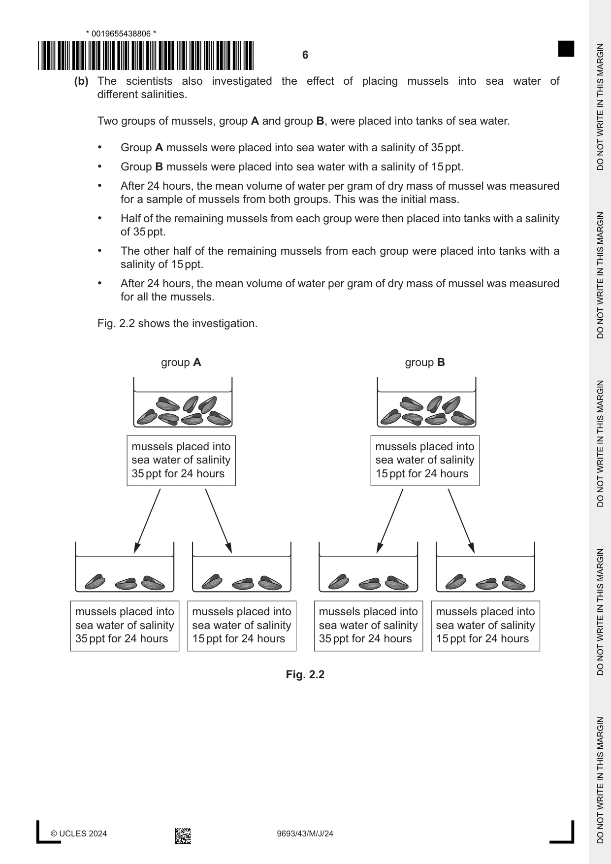
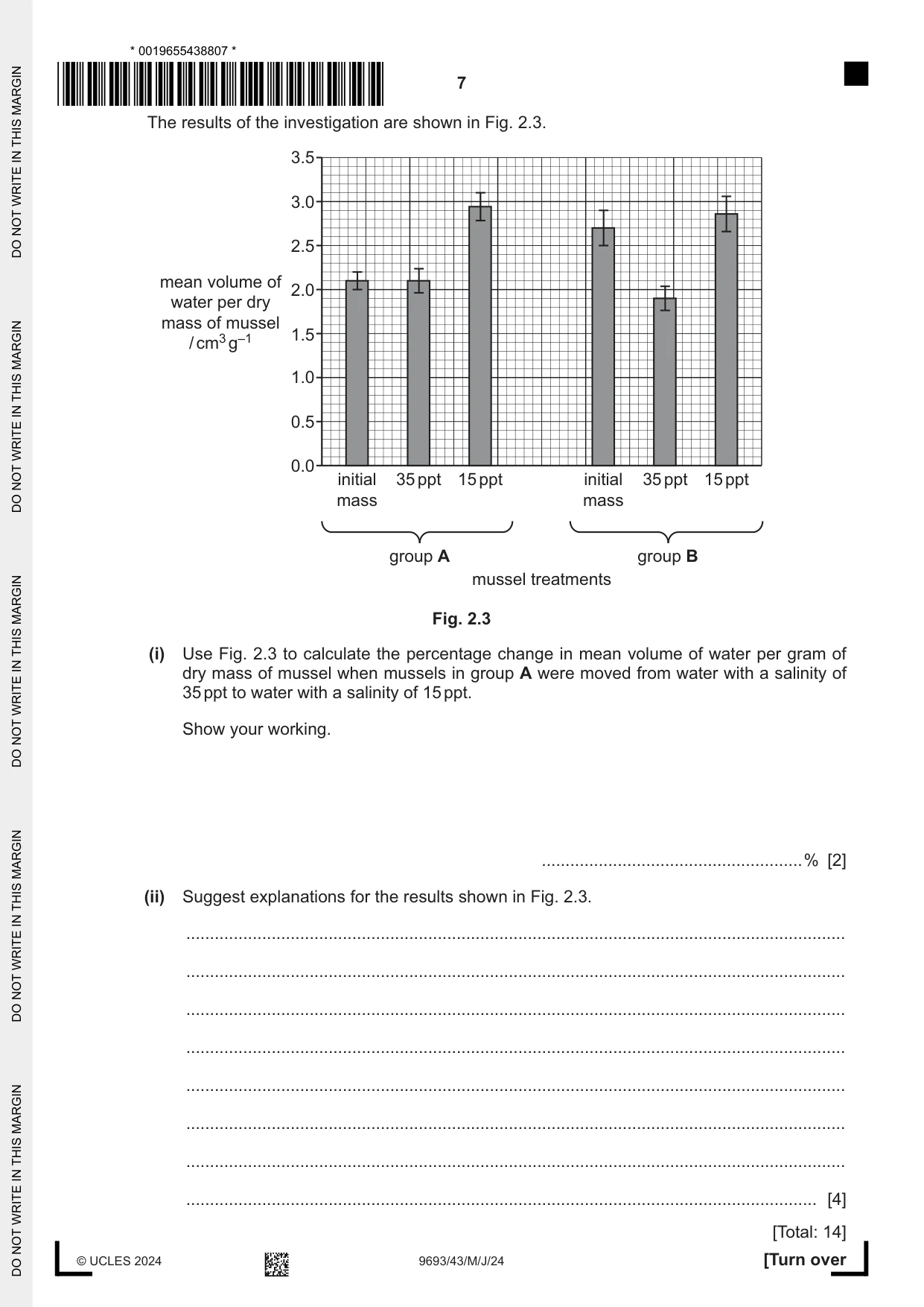
2 Killifish are euryhaline fish that are able to osmoregulate. (a) (i) State what is meant by the term euryhaline. ........................................................................................................................................... ..................................................................................................................................... [1] Scientists kept killifish in sea water with a salinity of 35 parts per thousand (ppt) for one week. The fish were then placed into fresh water. The scientists measured the rate of breakdown of ATP in gill cells and body skin cells of the killifish over one week. Energy is released when ATP is broken down. The results are shown in Fig. 2.1. 5.0 4.5 gill cells 4.0 3.5 3.0 rate of ATP breakdown 2.5 / mmol ATP g–1 h–1 2.0 body skin cells 1.5 1.0 0.5 0.0 0 1 2 3 4 5 6 7 8 time / days fish placed into fresh water Fig. 2.1 (ii) Describe the change in the rate of breakdown of ATP by the gill cells after placing the fish into fresh water. ........................................................................................................................................... ........................................................................................................................................... ........................................................................................................................................... ..................................................................................................................................... [2] (iii) Suggest an explanation for the change in the rate of breakdown of ATP after placing the killifish into fresh water. ........................................................................................................................................... ........................................................................................................................................... ........................................................................................................................................... ........................................................................................................................................... ........................................................................................................................................... ........................................................................................................................................... ........................................................................................................................................... ..................................................................................................................................... [4] (iv) Suggest why the scientists investigated the response of body skin cells as well as of gill cells. ........................................................................................................................................... ..................................................................................................................................... [1] (b) The scientists also investigated the effect of placing mussels into sea water of different salinities. Two groups of mussels, group A and group B, were placed into tanks of sea water. • Group A mussels were placed into sea water with a salinity of 35 ppt. • Group B mussels were placed into sea water with a salinity of 15 ppt. • After 24 hours, the mean volume of water per gram of dry mass of mussel was measured for a sample of mussels from both groups. This was the initial mass. • Half of the remaining mussels from each group were then placed into tanks with a salinity of 35 ppt. • The other half of the remaining mussels from each group were placed into tanks with a salinity of 15 ppt. • After 24 hours, the mean volume of water per gram of dry mass of mussel was measured for all the mussels. Fig. 2.2 shows the investigation. group A group B mussels placed into mussels placed into sea water of salinity sea water of salinity 35ppt for 24 hours 15ppt for 24 hours mussels placed into mussels placed into mussels placed into mussels placed into sea water of salinity sea water of salinity sea water of salinity sea water of salinity 35ppt for 24 hours 15ppt for 24 hours 35ppt for 24 hours 15ppt for 24 hours Fig. 2.2 The results of the investigation are shown in Fig. 2.3. 3.5 3.0 2.5 mean volume of 2.0 water per dry mass of mussel 1.5 / cm3 g–1 1.0 0.5 0.0 initial 35 ppt 15 ppt initial 35 ppt 15 ppt mass mass group A group B mussel treatments Fig. 2.3 (i) Use Fig. 2.3 to calculate the percentage change in mean volume of water per gram of dry mass of mussel when mussels in group A were moved from water with a salinity of 35 ppt to water with a salinity of 15 ppt. Show your working. .......................................................% [2] (ii) Suggest explanations for the results shown in Fig. 2.3. ........................................................................................................................................... ........................................................................................................................................... ........................................................................................................................................... ........................................................................................................................................... ........................................................................................................................................... ........................................................................................................................................... ........................................................................................................................................... ..................................................................................................................................... [4] [Total: 14]

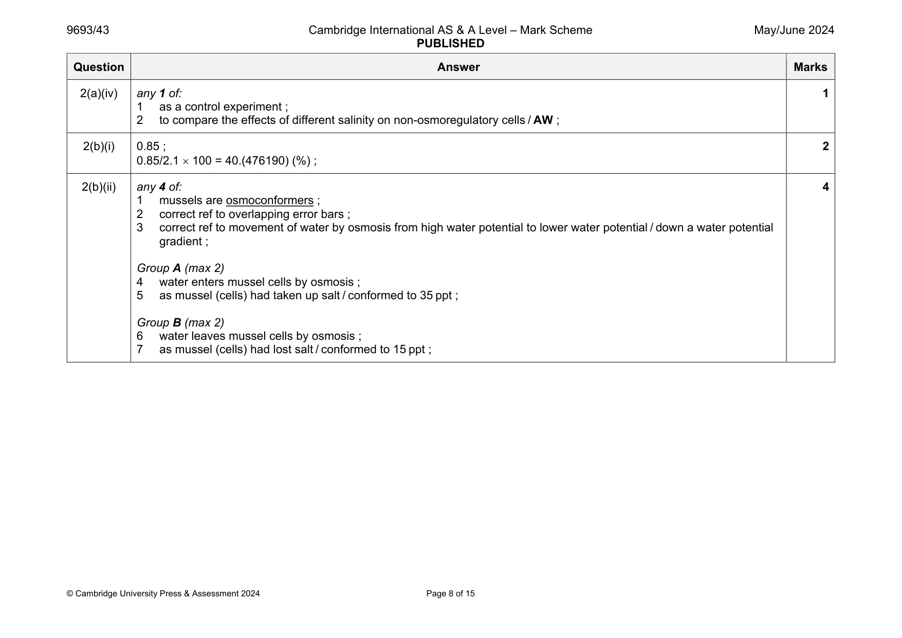
Mark scheme: 2(a)(i) (organisms) that can live in salt and fresh water / can live in a range of salinities / AW ; 1 2(a)(ii) any 2 of: 1 (steep) increase ; 2 levels off after one day/fluctuates after one day / goes up and down after one day / decrease and increase after one day / AW ; 3 accept correct manipulated data ; 2 2(a)(iii) any 4 of: 1 fish has lower water potential (than water) / (fresh) water has higher water potential than fish / AW ; 2 so water enter fish by osmosis / AW ; 3 (gill cells) move, salt / sodium / chloride / ions, into, body / blood ; 4 by active transport / active process (of salt) ; 5 so more energy (needs to be released) ; 6 as salt is lost from body via urine / diffusion / salt diffuses out of fish ; 7 maximum rate of, salt / sodium / chloride, pumping occurs after one day / AW ; 4 Question Answer Marks 2(a)(iv) any 1 of: 1 as a control experiment ; 2 to compare the effects of different salinity on non-osmoregulatory cells / AW ; 1 2(b)(i) 0.85 ; 0.85/2.1  100 = 40.(476190) (%) ; 2 2(b)(ii) any 4 of: 1 mussels are osmoconformers ; 2 correct ref to overlapping error bars ; 3 correct ref to movement of water by osmosis from high water potential to lower water potential / down a water potential gradient ; Group A (max 2) 4 water enters mussel cells by osmosis ; 5 as mussel (cells) had taken up salt / conformed to 35 ppt ; Group B (max 2) 6 water leaves mussel cells by osmosis ; 7 as mussel (cells) had lost salt / conformed to 15 ppt ; 4

More questions on Osmoregulation

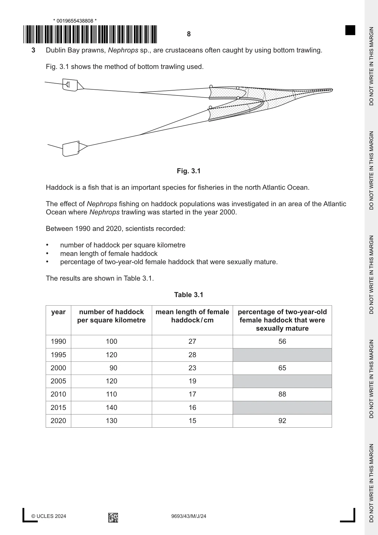
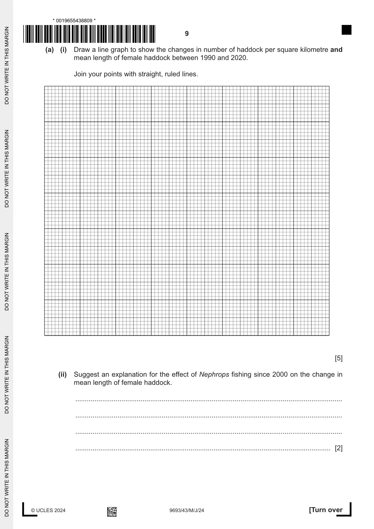
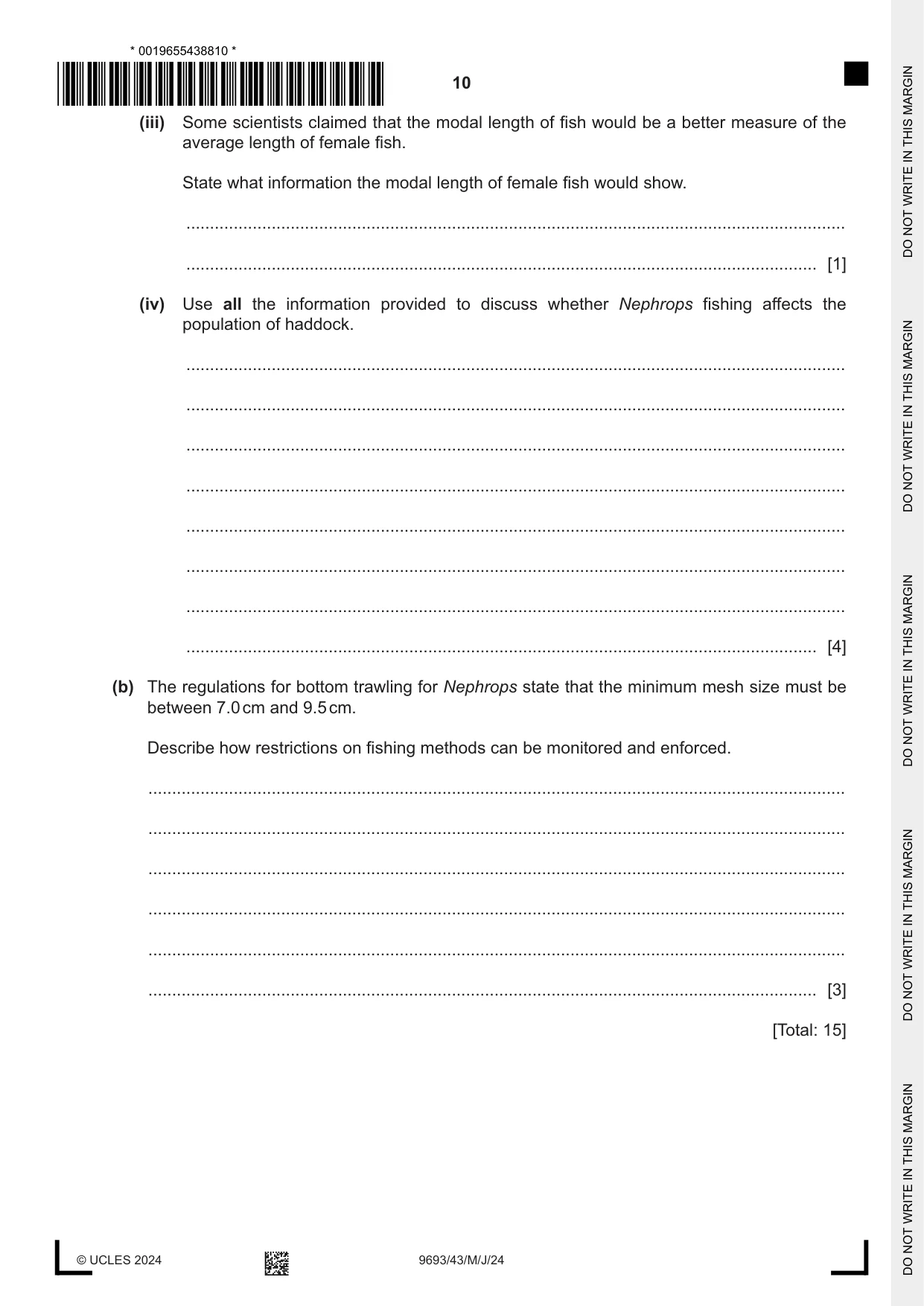
3 Dublin Bay prawns, Nephrops sp., are crustaceans often caught by using bottom trawling. Fig. 3.1 shows the method of bottom trawling used. Fig. 3.1 Haddock is a fish that is an important species for fisheries in the north Atlantic Ocean. The effect of Nephrops fishing on haddock populations was investigated in an area of the Atlantic Ocean where Nephrops trawling was started in the year 2000. Between 1990 and 2020, scientists recorded: • number of haddock per square kilometre • mean length of female haddock • percentage of two-year-old female haddock that were sexually mature. The results are shown in Table 3.1. Table 3.1 year number of haddock mean length of female percentage of two‑year‑old per square kilometre haddock / cm female haddock that were sexually mature 1990 100 27 56 1995 120 28 2000 90 23 65 2005 120 19 2010 110 17 88 2015 140 16 2020 130 15 92 (a) (i) Draw a line graph to show the changes in number of haddock per square kilometre and mean length of female haddock between 1990 and 2020. Join your points with straight, ruled lines. [5] (ii) Suggest an explanation for the effect of Nephrops fishing since 2000 on the change in mean length of female haddock. ........................................................................................................................................... ........................................................................................................................................... ........................................................................................................................................... ..................................................................................................................................... [2] (iii) Some scientists claimed that the modal length of fish would be a better measure of the average length of female fish. State what information the modal length of female fish would show. ........................................................................................................................................... ..................................................................................................................................... [1] (iv) Use all the information provided to discuss whether Nephrops fishing affects the population of haddock. ........................................................................................................................................... ........................................................................................................................................... ........................................................................................................................................... ........................................................................................................................................... ........................................................................................................................................... ........................................................................................................................................... ........................................................................................................................................... ..................................................................................................................................... [4] (b) The regulations for bottom trawling for Nephrops state that the minimum mesh size must be between 7.0 cm and 9.5 cm. Describe how restrictions on fishing methods can be monitored and enforced. ................................................................................................................................................... ................................................................................................................................................... ................................................................................................................................................... ................................................................................................................................................... ................................................................................................................................................... ............................................................................................................................................. [3] [Total: 15]

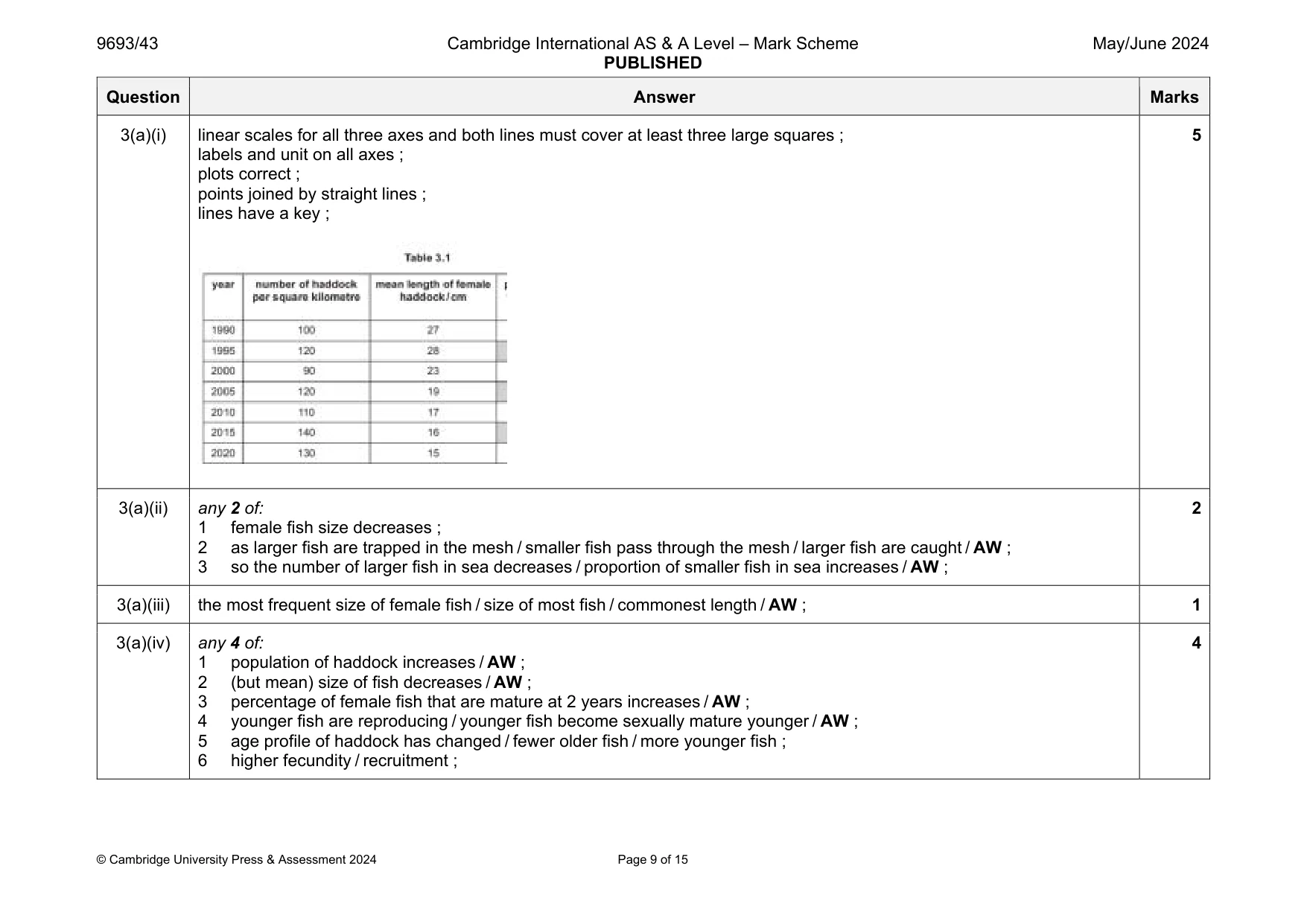
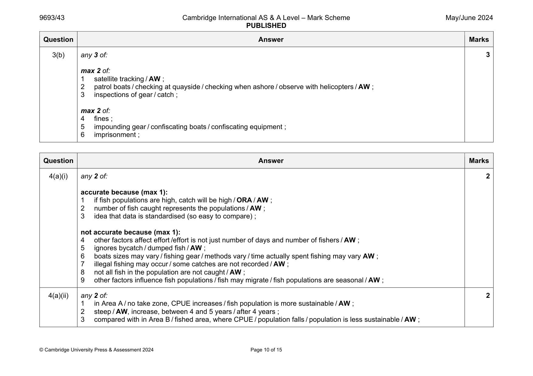
Mark scheme: 3(a)(i) linear scales for all three axes and both lines must cover at least three large squares ; labels and unit on all axes ; plots correct ; points joined by straight lines ; lines have a key ; 5 3(a)(ii) any 2 of: 1 female fish size decreases ; 2 as larger fish are trapped in the mesh / smaller fish pass through the mesh / larger fish are caught / AW ; 3 so the number of larger fish in sea decreases / proportion of smaller fish in sea increases / AW ; 2 3(a)(iii) the most frequent size of female fish / size of most fish / commonest length / AW ; 1 3(a)(iv) any 4 of: 1 population of haddock increases / AW ; 2 (but mean) size of fish decreases / AW ; 3 percentage of female fish that are mature at 2 years increases / AW ; 4 younger fish are reproducing / younger fish become sexually mature younger / AW ; 5 age profile of haddock has changed / fewer older fish / more younger fish ; 6 higher fecundity / recruitment ; 4 Question Answer Marks 3(b) any 3 of: max 2 of: 1 satellite tracking / AW ; 2 patrol boats / checking at quayside / checking when ashore / observe with helicopters / AW ; 3 inspections of gear / catch ; max 2 of: 4 fines ; 5 impounding gear / confiscating boats / confiscating equipment ; 6 imprisonment ; 3

More questions on Sustainable fisheries

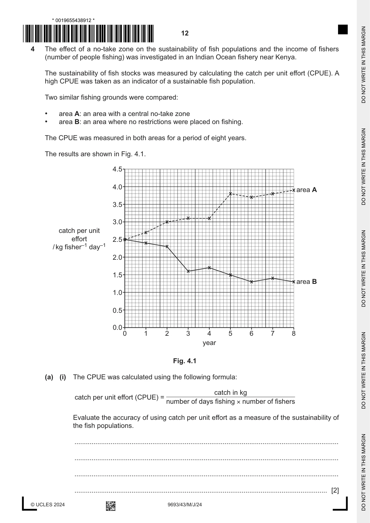
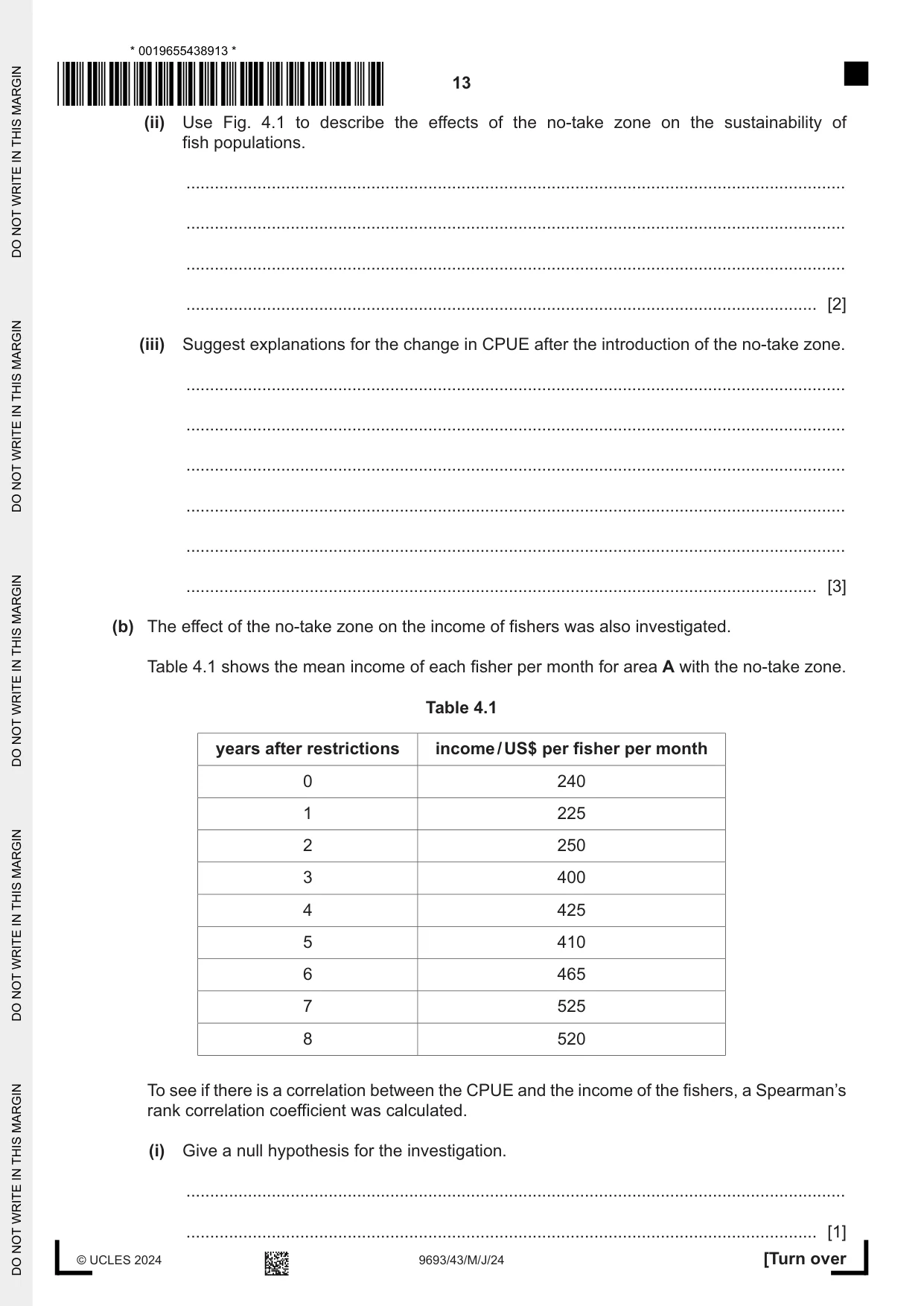
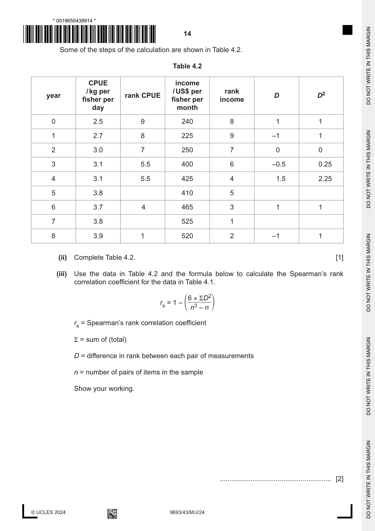
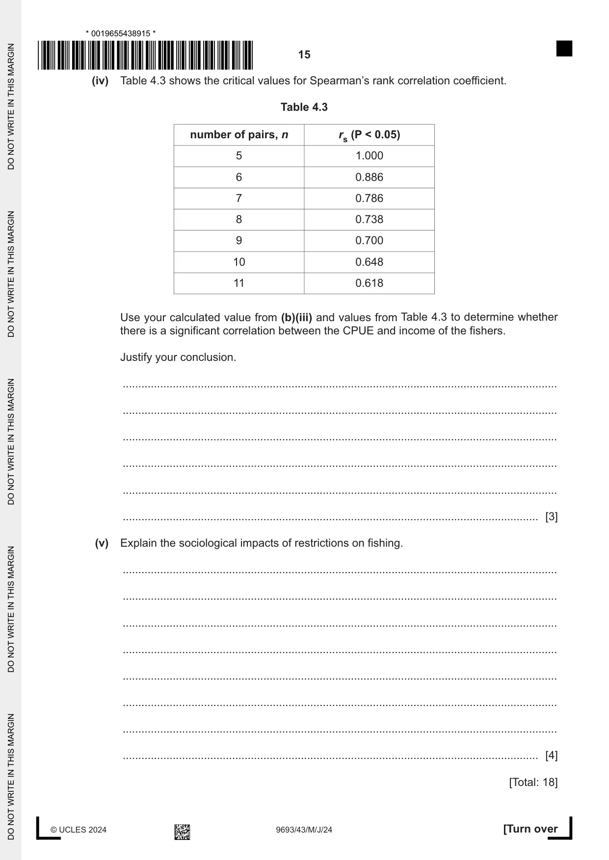
4 The effect of a no-take zone on the sustainability of fish populations and the income of fishers (number of people fishing) was investigated in an Indian Ocean fishery near Kenya. The sustainability of fish stocks was measured by calculating the catch per unit effort (CPUE). A high CPUE was taken as an indicator of a sustainable fish population. Two similar fishing grounds were compared: • area A: an area with a central no-take zone • area B: an area where no restrictions were placed on fishing. The CPUE was measured in both areas for a period of eight years. The results are shown in Fig. 4.1. 4.5 4.0 area A 3.5 3.0 catch per unit effort 2.5 / kg fisher–1 day–1 2.0 1.5 area B 1.0 0.5 0.0 0 1 2 3 4 5 6 7 8 year Fig. 4.1 (a) (i) The CPUE was calculated using the following formula: catch in kg catch per unit effort (CPUE) = number of days fishing × number of fishers Evaluate the accuracy of using catch per unit effort as a measure of the sustainability of the fish populations. ........................................................................................................................................... ........................................................................................................................................... ........................................................................................................................................... ..................................................................................................................................... [2] (ii) Use Fig. 4.1 to describe the effects of the no-take zone on the sustainability of fish populations. ........................................................................................................................................... ........................................................................................................................................... ........................................................................................................................................... ..................................................................................................................................... [2] (iii) Suggest explanations for the change in CPUE after the introduction of the no-take zone. ........................................................................................................................................... ........................................................................................................................................... ........................................................................................................................................... ........................................................................................................................................... ........................................................................................................................................... ..................................................................................................................................... [3] (b) The effect of the no-take zone on the income of fishers was also investigated. Table 4.1 shows the mean income of each fisher per month for area A with the no-take zone. Table 4.1 years after restrictions income / US$ per fisher per month 0 240 1 225 2 250 3 400 4 425 5 410 6 465 7 525 8 520 To see if there is a correlation between the CPUE and the income of the fishers, a Spearman’s rank correlation coefficient was calculated. (i) Give a null hypothesis for the investigation. ........................................................................................................................................... ..................................................................................................................................... [1] Some of the steps of the calculation are shown in Table 4.2. Table 4.2 CPUE income / kg per / US$ per rank year rank CPUE D D2 fisher per fisher per income day month 0 2.5 9 240 8 1 1 1 2.7 8 225 9 –1 1 2 3.0 7 250 7 0 0 3 3.1 5.5 400 6 –0.5 0.25 4 3.1 5.5 425 4 1.5 2.25 5 3.8 410 5 6 3.7 4 465 3 1 1 7 3.8 525 1 8 3.9 1 520 2 –1 1 (ii) Complete Table 4.2. [1] (iii) Use the data in Table 4.2 and the formula below to calculate the Spearman’s rank correlation coefficient for the data in Table 4.1. 6 × ΣD2 rs = 1 – 1 n3 – n 2 rs = Spearman’s rank correlation coefficient Σ = sum of (total) D = difference in rank between each pair of measurements n = number of pairs of items in the sample Show your working. .......................................................... [2] (iv) Table 4.3 shows the critical values for Spearman’s rank correlation coefficient. Table 4.3 number of pairs, n rs (P < 0.05) 5 1.000 6 0.886 7 0.786 8 0.738 9 0.700 10 0.648 11 0.618 Use your calculated value from (b)(iii) and values from Table 4.3 to determine whether there is a significant correlation between the CPUE and income of the fishers. Justify your conclusion. ........................................................................................................................................... ........................................................................................................................................... ........................................................................................................................................... ........................................................................................................................................... ........................................................................................................................................... ..................................................................................................................................... [3] (v) Explain the sociological impacts of restrictions on fishing. ........................................................................................................................................... ........................................................................................................................................... ........................................................................................................................................... ........................................................................................................................................... ........................................................................................................................................... ........................................................................................................................................... ........................................................................................................................................... ..................................................................................................................................... [4] [Total: 18]

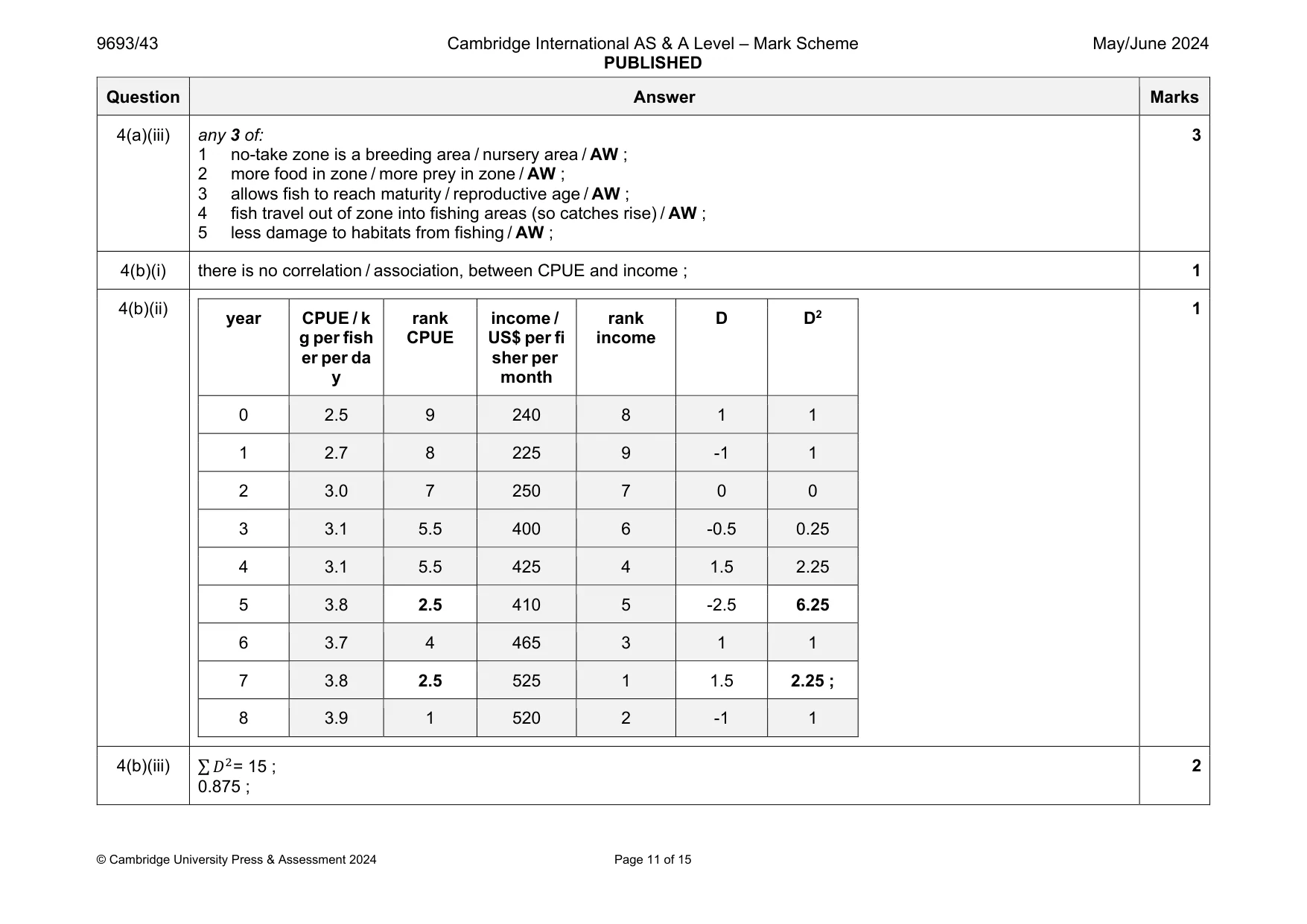
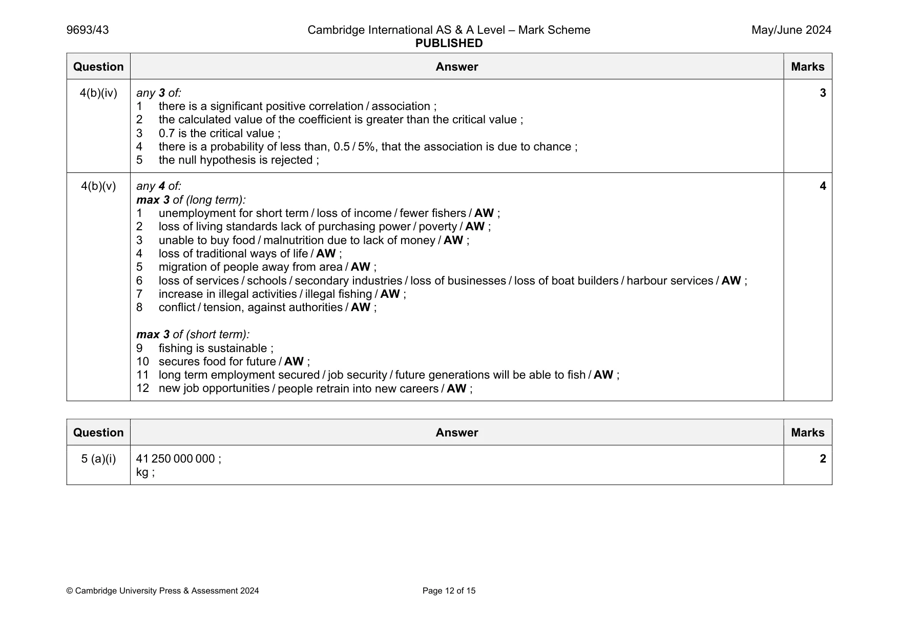
Mark scheme: 4(a)(i) any 2 of: accurate because (max 1): 1 if fish populations are high, catch will be high / ORA / AW ; 2 number of fish caught represents the populations / AW ; 3 idea that data is standardised (so easy to compare) ; not accurate because (max 1): 4 other factors affect effort /effort is not just number of days and number of fishers / AW ; 5 ignores bycatch / dumped fish / AW ; 6 boats sizes may vary / fishing gear / methods vary / time actually spent fishing may vary AW ; 7 illegal fishing may occur / some catches are not recorded / AW ; 8 not all fish in the population are not caught / AW ; 9 other factors influence fish populations / fish may migrate / fish populations are seasonal / AW ; 2 4(a)(ii) any 2 of: 1 in Area A / no take zone, CPUE increases / fish population is more sustainable / AW ; 2 steep / AW, increase, between 4 and 5 years / after 4 years ; 3 compared with in Area B / fished area, where CPUE / population falls / population is less sustainable / AW ; 2 Question Answer Marks 4(a)(iii) any 3 of: 1 no-take zone is a breeding area / nursery area / AW ; 2 more food in zone / more prey in zone / AW ; 3 allows fish to reach maturity / reproductive age / AW ; 4 fish travel out of zone into fishing areas (so catches rise) / AW ; 5 less damage to habitats from fishing / AW ; 3 4(b)(i) there is no correlation / association, between CPUE and income ; 1 4(b)(ii) year CPUE / k g per fish er per da y rank CPUE income / US$ per fi sher per month rank income D D2 0 2.5 9 240 8 1 1 1 2.7 8 225 9 -1 1 2 3.0 7 250 7 0 0 3 3.1 5.5 400 6 -0.5 0.25 4 3.1 5.5 425 4 1.5 2.25 5 3.8 2.5 410 5 -2.5 6.25 6 3.7 4 465 3 1 1 7 3.8 2.5 525 1 1.5 2.25 ; 8 3.9 1 520 2 -1 1 1 4(b)(iii) ∑𝐷ଶ= 15 ; 0.875 ; 2 Question Answer Marks 4(b)(iv) any 3 of: 1 there is a significant positive correlation / association ; 2 the calculated value of the coefficient is greater than the critical value ; 3 0.7 is the critical value ; 4 there is a probability of less than, 0.5 / 5%, that the association is due to chance ; 5 the null hypothesis is rejected ; 3 4(b)(v) any 4 of: max 3 of (long term): 1 unemployment for short term / loss of income / fewer fishers / AW ; 2 loss of living standards lack of purchasing power / poverty / AW ; 3 unable to buy food / malnutrition due to lack of money / AW ; 4 loss of traditional ways of life / AW ; 5 migration of people away from area / AW ; 6 loss of services / schools / secondary industries / loss of businesses / loss of boat builders / harbour services / AW ; 7 increase in illegal activities / illegal fishing / AW ; 8 conflict / tension, against authorities / AW ; max 3 of (short term): 9 fishing is sustainable ; 10 secures food for future / AW ; 11 long term employment secured / job security / future generations will be able to fish / AW ; 12 new job opportunities / people retrain into new careers / AW ; 4

More questions on Sustainable fisheries

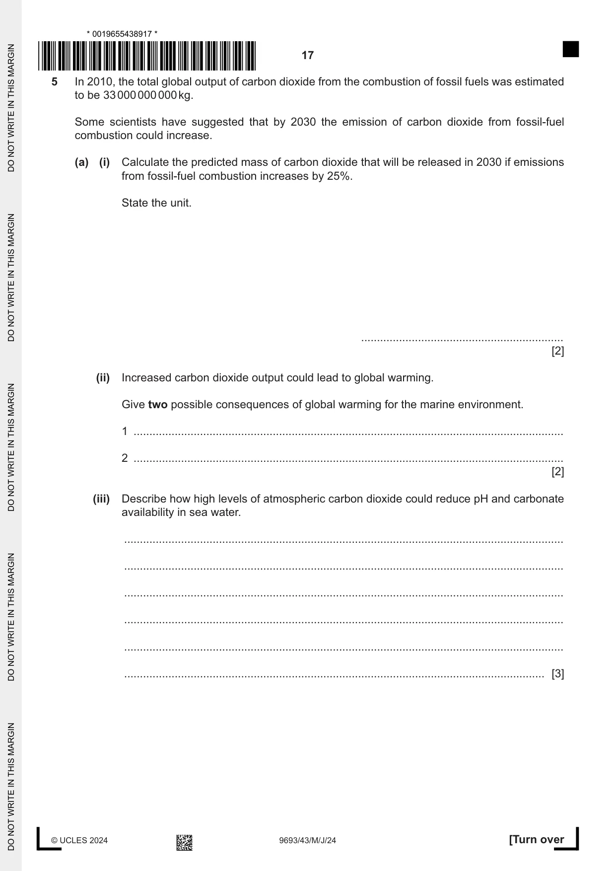
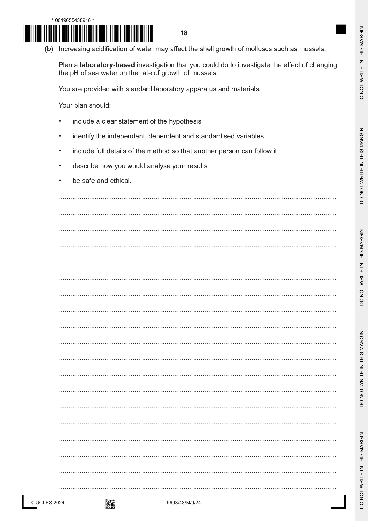
5 In 2010, the total global output of carbon dioxide from the combustion of fossil fuels was estimated to be 33 000 000 000 kg. Some scientists have suggested that by 2030 the emission of carbon dioxide from fossil-fuel combustion could increase. (a) (i) Calculate the predicted mass of carbon dioxide that will be released in 2030 if emissions from fossil-fuel combustion increases by 25%. State the unit. ................................................................ [2] (ii) Increased carbon dioxide output could lead to global warming. Give two possible consequences of global warming for the marine environment. 1 ........................................................................................................................................ 2 ........................................................................................................................................ [2] (iii) Describe how high levels of atmospheric carbon dioxide could reduce pH and carbonate availability in sea water. ........................................................................................................................................... ........................................................................................................................................... ........................................................................................................................................... ........................................................................................................................................... ........................................................................................................................................... ..................................................................................................................................... [3] (b) Increasing acidification of water may affect the shell growth of molluscs such as mussels. Plan a laboratory‑based investigation that you could do to investigate the effect of changing the pH of sea water on the rate of growth of mussels. You are provided with standard laboratory apparatus and materials. Your plan should: • include a clear statement of the hypothesis • identify the independent, dependent and standardised variables • include full details of the method so that another person can follow it • describe how you would analyse your results • be safe and ethical. ................................................................................................................................................... ................................................................................................................................................... ................................................................................................................................................... ................................................................................................................................................... ................................................................................................................................................... ................................................................................................................................................... ................................................................................................................................................... ................................................................................................................................................... ................................................................................................................................................... ................................................................................................................................................... ................................................................................................................................................... ................................................................................................................................................... ................................................................................................................................................... ................................................................................................................................................... ................................................................................................................................................... ................................................................................................................................................... ................................................................................................................................................... ................................................................................................................................................... ................................................................................................................................................... ................................................................................................................................................... ................................................................................................................................................... ................................................................................................................................................... ................................................................................................................................................... ................................................................................................................................................... ................................................................................................................................................... ................................................................................................................................................... ................................................................................................................................................... ................................................................................................................................................... ................................................................................................................................................... ................................................................................................................................................... ................................................................................................................................................... ........................................................................................................................................... [12] [Total: 19]

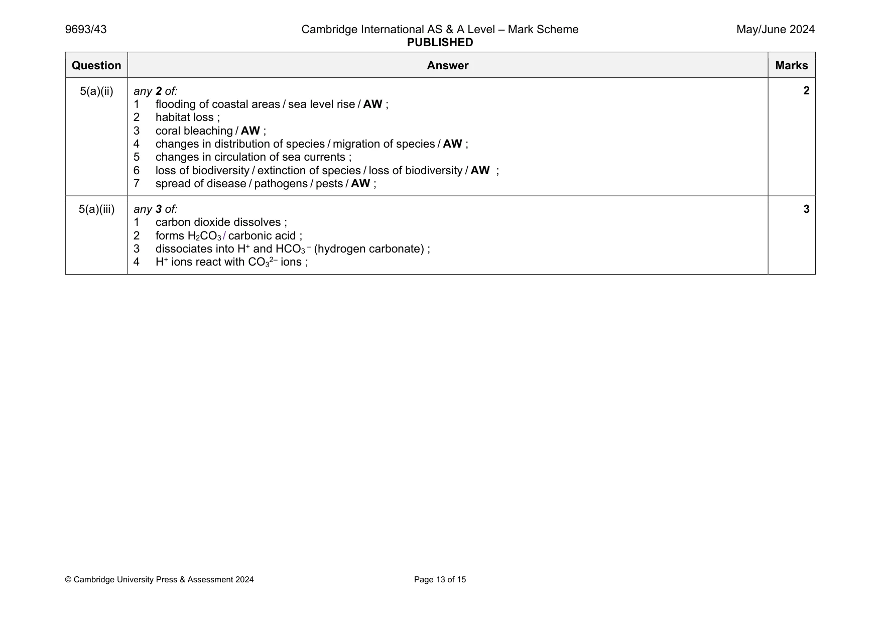
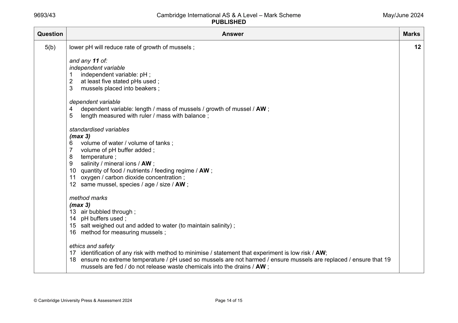
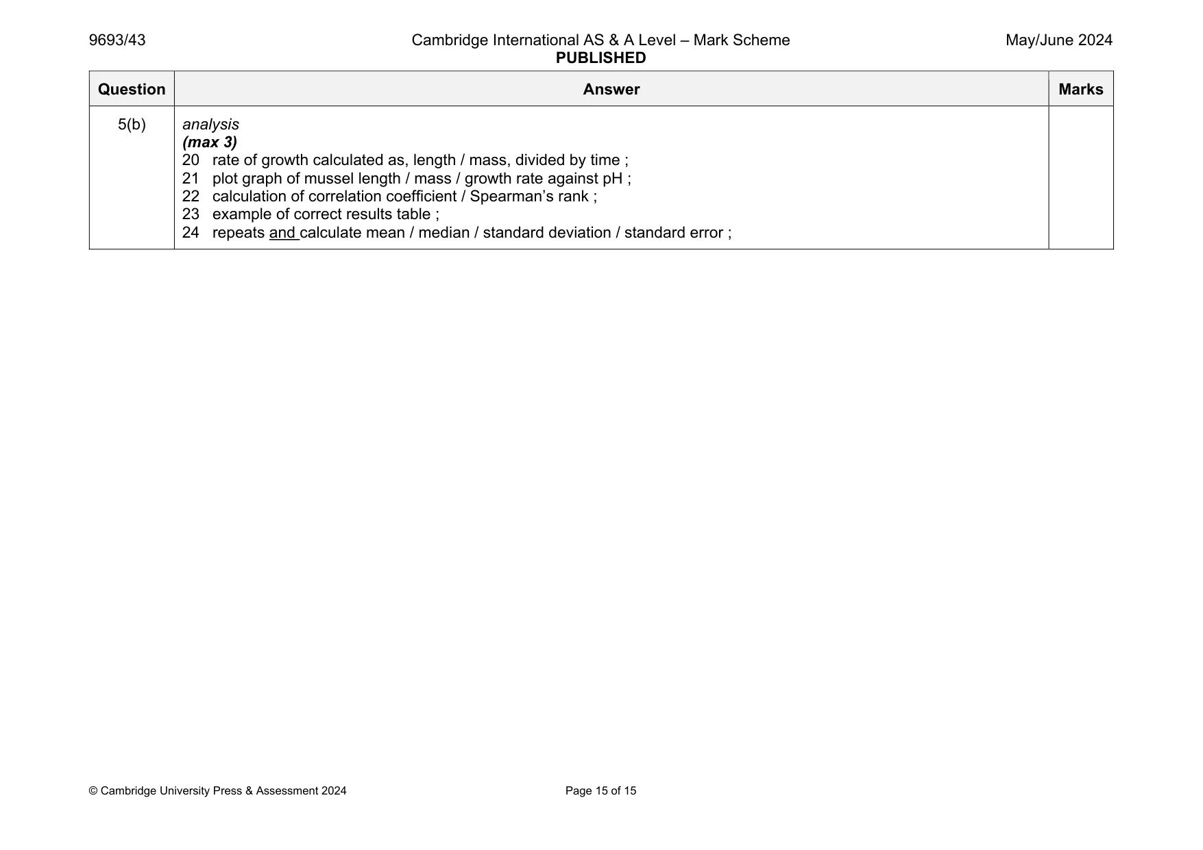
Mark scheme: 5 (a)(i) 41 250 000 000 ; kg ; 2 Question Answer Marks 5(a)(ii) any 2 of: 1 flooding of coastal areas / sea level rise / AW ; 2 habitat loss ; 3 coral bleaching / AW ; 4 changes in distribution of species / migration of species / AW ; 5 changes in circulation of sea currents ; 6 loss of biodiversity / extinction of species / loss of biodiversity / AW ; 7 spread of disease / pathogens / pests / AW ; 2 5(a)(iii) any 3 of: 1 carbon dioxide dissolves ; 2 forms H2CO3 / carbonic acid ; 3 dissociates into H+ and HCO3 – (hydrogen carbonate) ; 4 H+ ions react with CO32– ions ; 3 Question Answer Marks 5(b) lower pH will reduce rate of growth of mussels ; and any 11 of: independent variable 1 independent variable: pH ; 2 at least five stated pHs used ; 3 mussels placed into beakers ; dependent variable 4 dependent variable: length / mass of mussels / growth of mussel / AW ; 5 length measured with ruler / mass with balance ; standardised variables (max 3) 6 volume of water / volume of tanks ; 7 volume of pH buffer added ; 8 temperature ; 9 salinity / mineral ions / AW ; 10 quantity of food / nutrients / feeding regime / AW ; 11 oxygen / carbon dioxide concentration ; 12 same mussel, species / age / size / AW ; method marks (max 3) 13 air bubbled through ; 14 pH buffers used ; 15 salt weighed out and added to water (to maintain salinity) ; 16 method for measuring mussels ; ethics and safety 17 identification of any risk with method to minimise / statement that experiment is low risk / AW; 18 ensure no extreme temperature / pH used so mussels are not harmed / ensure mussels are replaced / ensure that 19 mussels are fed / do not release waste chemicals into the drains / AW ; 12 Question Answer Marks 5(b) analysis (max 3) 20 rate of growth calculated as, length / mass, divided by time ; 21 plot graph of mussel length / mass / growth rate against pH ; 22 calculation of correlation coefficient / Spearman’s rank ; 23 example of correct results table ; 24 repeats and calculate mean / median / standard deviation / standard error ;

More questions on Ocean acidification