Questions as text
Q1 · A student is investigating the motion of a small steel ball in cooking oil 9702/52 Feb/March 2019
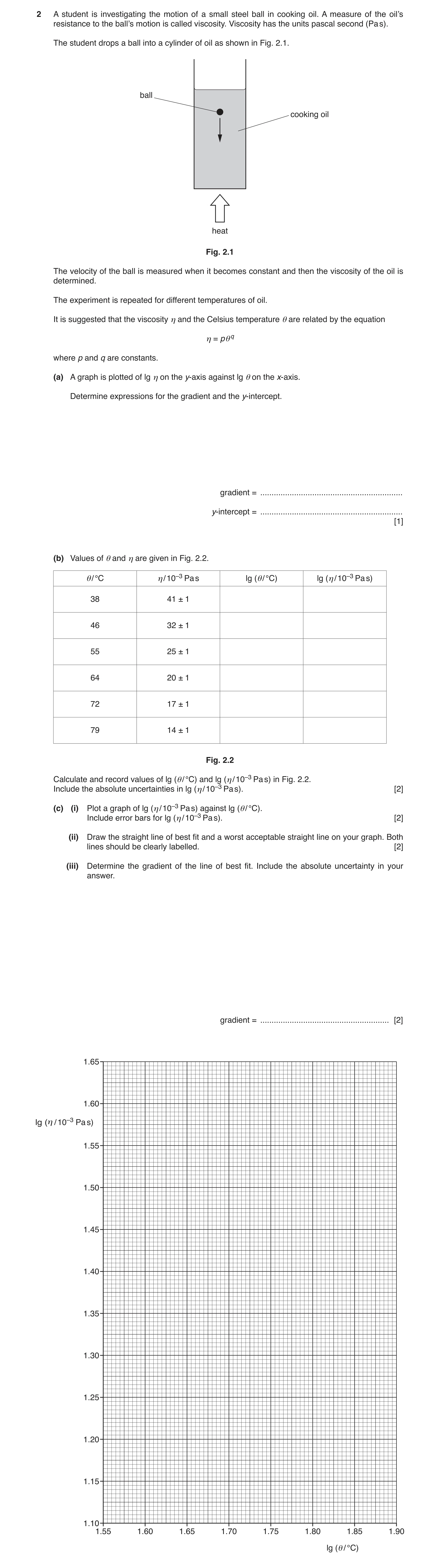
2 A student is investigating the motion of a small steel ball in cooking oil. A measure of the oil’s resistance to the ball’s motion is called viscosity. Viscosity has the units pascal second (Pa s). The student drops a ball into a cylinder of oil as shown in Fig. 2.1. ball cooking oil heat Fig. 2.1 The velocity of the ball is measured when it becomes constant and then the viscosity of the oil is determined. The experiment is repeated for different temperatures of oil. It is suggested that the viscosity η and the Celsius temperature θ are related by the equation η = p θ q where p and q are constants. (a) A graph is plotted of lg η on the y-axis against lg θ on the x-axis. Determine expressions for the gradient and the y-intercept. gradient = … y-intercept = … [1] (b) Values of θ and η are given in Fig. 2.2. θ/ °C η/ 10–3 Pa s lg (θ/ °C) lg (η/ 10–3 Pa s) 38 41 ± 1 46 32 ± 1 55 25 ± 1 64 20 ± 1 72 17 ± 1 79 14 ± 1 Fig. 2.2 Calculate and record values of lg (θ/ °C) and lg (η/ 10–3 Pa s) in Fig. 2.2. Include the absolute uncertainties in lg (η/ 10–3 Pa s). [2] (c) (i) Plot a graph of lg (η/ 10–3 Pa s) against lg (θ/ °C). Include error bars for lg (η/ 10–3 Pa s). [2] (ii) Draw the straight line of best fit and a worst acceptable straight line on your graph. Both lines should be clearly labelled. [2] (iii) Determine the gradient of the line of best fit. Include the absolute uncertainty in your answer. gradient = … [2]
9 marks
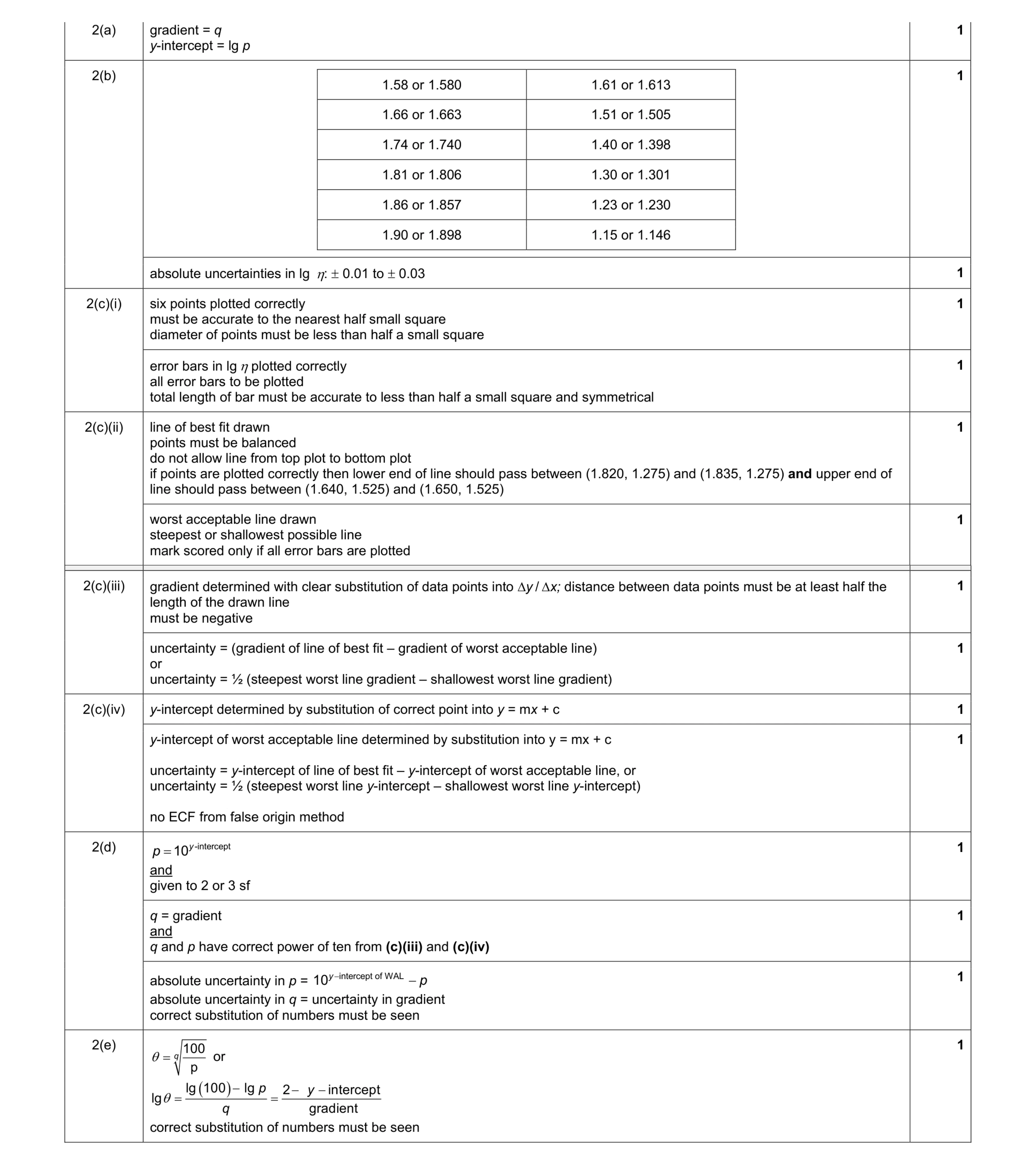
Mark scheme: 2(a) gradient = q y-intercept = lg p 1 2(b) 1.58 or 1.580 1.61 or 1.613 1.66 or 1.663 1.51 or 1.505 1.74 or 1.740 1.40 or 1.398 1.81 or 1.806 1.30 or 1.301 1.86 or 1.857 1.23 or 1.230 1.90 or 1.898 1.15 or 1.146 1 absolute uncertainties in lg η: ± 0.01 to ± 0.03 1 2(c)(i) six points plotted correctly must be accurate to the nearest half small square diameter of points must be less than half a small square 1 error bars in lg η plotted correctly all error bars to be plotted total length of bar must be accurate to less than half a small square and symmetrical 1 2(c)(ii) line of best fit drawn points must be balanced do not allow line from top plot to bottom plot if points are plotted correctly then lower end of line should pass between (1.820, 1.275) and (1.835, 1.275) and upper end of line should pass between (1.640, 1.525) and (1.650, 1.525) 1 worst acceptable line drawn steepest or shallowest possible line mark scored only if all error bars are plotted 1 Question Answer Marks 2(c)(iii) gradient determined with clear substitution of data points into ∆y / ∆x; distance between data points must be at least half the length of the drawn line must be negative 1 uncertainty = (gradient of line of best fit – gradient of worst acceptable line) or uncertainty = ½ (steepest worst line gradient – shallowest worst line gradient) 1 2(c)(iv) y-intercept determined by substitution of correct point into y = mx + c 1 y-intercept of worst acceptable line determined by substitution into y = mx + c uncertainty = y-intercept of line of best fit – y-intercept of worst acceptable line, or uncertainty = ½ (steepest worst line y-intercept – shallowest worst line y-intercept) no ECF from false origin method 1 2(d) -intercept 10y p = and given to 2 or 3 sf 1 q = gradient and q and p have correct power of ten from (c)(iii) and (c)(iv) 1 absolute uncertainty in p = intercept of WAL 10y p − − absolute uncertainty in q = uncertainty in gradient correct substitution of numbers must be seen 1 2(e) 100 p q θ = or ( ) lg 100 lg 2 intercept lg gradient p y q θ − − − = = correct substitution of numbers must be seen 1
This question in 9702/52 Feb/March 2019
Q2 · When a light plastic ball is placed in a vertical column of moving air, the ball becomes… 9702/51 Oct/Nov 2019
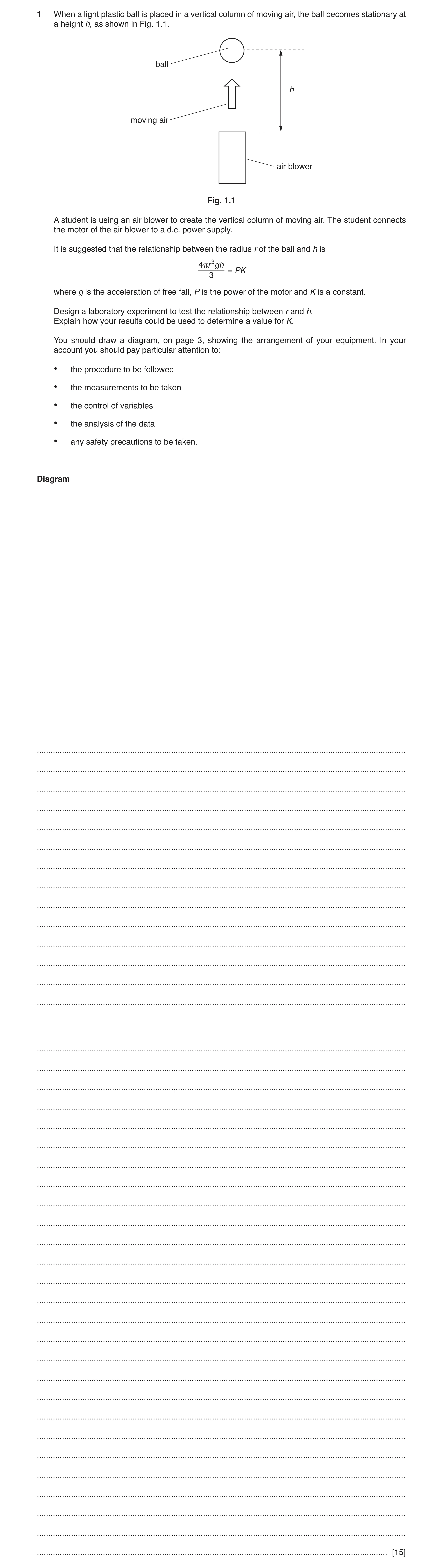
1 When a light plastic ball is placed in a vertical column of moving air, the ball becomes stationary at a height h, as shown in Fig. 1.1. ball h moving air air blower Fig. 1.1 A student is using an air blower to create the vertical column of moving air. The student connects the motor of the air blower to a d.c. power supply. It is suggested that the relationship between the radius r of the ball and h is 4 r r 3 gh = PK 3 where g is the acceleration of free fall, P is the power of the motor and K is a constant. Design a laboratory experiment to test the relationship between r and h. Explain how your results could be used to determine a value for K. You should draw a diagram, on page 3, showing the arrangement of your equipment. In your account you should pay particular attention to: • the procedure to be followed • the measurements to be taken • the control of variables • the analysis of the data • any safety precautions to be taken. Diagram … … … … … … … … … … … … … … … … … … … … … … … … … … … … … … … … … … … … … … … … … [15]
15 marks
Mark scheme: 1 Defining the problem r is the independent variable and h is the dependent variable or vary r and measure/determine h 1 keep P constant 1 Methods of data collection labelled diagram of workable experiment including: • labelled air blower • labelled ball vertically (by eye) above the blower • vertical (by eye) rule at least from top of blower to ball 1 circuit diagram to determine P, e.g. voltmeter and ammeter connected to motor and power supply or wattmeter connected to motor and power supply 1 use of micrometer/calipers/rule to measure diameter of ball 1 measure the distance between the top/middle/bottom of the ball and the top of the blower 1 Method of Analysis plot a graph of h against 1 / r3 (or lg h against lg r) 1 relationship valid if a straight line through (0,0) (for lg h against lg r straight line with gradient = –3) 1 4 gradient 3 g K P π × = (for lg h against lg r, intercept 4 10 3 y g K P − π × = ) 1 Question Answer Marks 1 Additional detail including safety considerations D1 use large box/tray to collect ball (to prevent ball rolling on floor/bouncing) or reasoned method to avoid draughts, e.g. switch off fans, close windows, use a screen 6 D2 method to determine P from correct circuit, e.g. P = I × V or use wattmeter to measure P D3 stand on bench with clamped rule vertically to measure vertical distance D4 method to ensure clamped rule to measure h is vertical, e.g. correctly positioned set square indicated at right angles between the rule and the horizontal surface or plumb line shown in appropriate position D5 r = d / 2 when diameter measured D6 repeat diameter measurement in different directions and find average D7 repeat experiment for each value of r and determine average h D8 method to determine h, e.g. h = reading top of ball – r – top of blower or h = reading bottom of ball + r – top of blower or h = (distance from top of ball to top of blower + distance from bottom of ball to top of blower) / 2 D9 wait for the ball to become stationary (vertically) D10 video (camera) shown level with elevated ball and description of playback frame-by-frame or slow motion
This question in 9702/51 Oct/Nov 2019
Q3 · A student is investigating the oscillations of a mass attached to two springs connected… 9702/51 Oct/Nov 2019
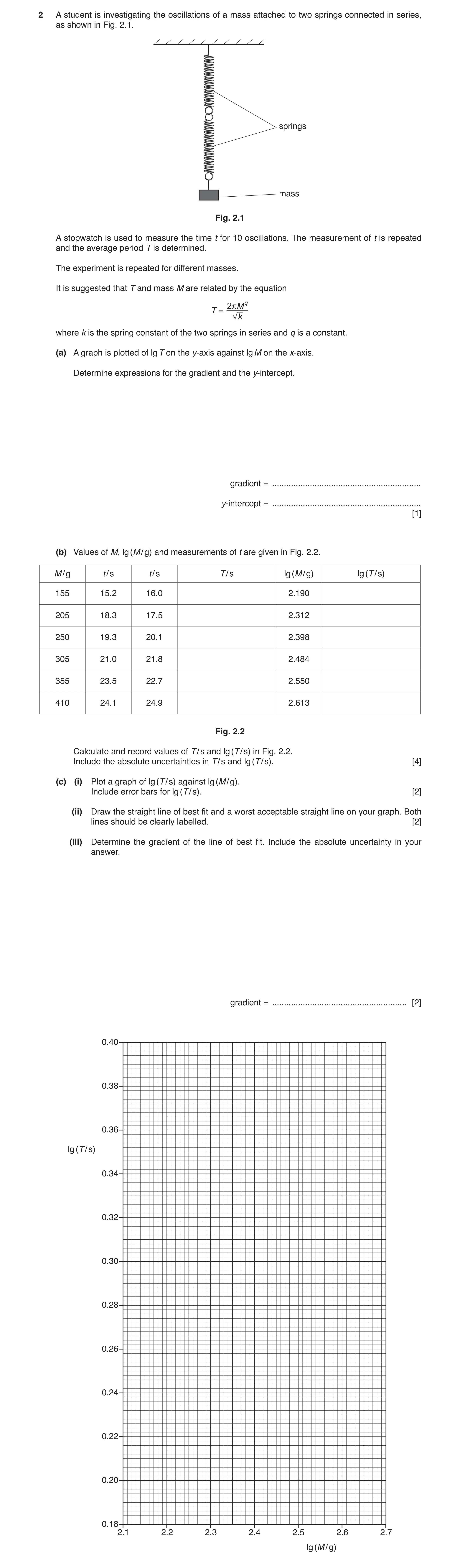
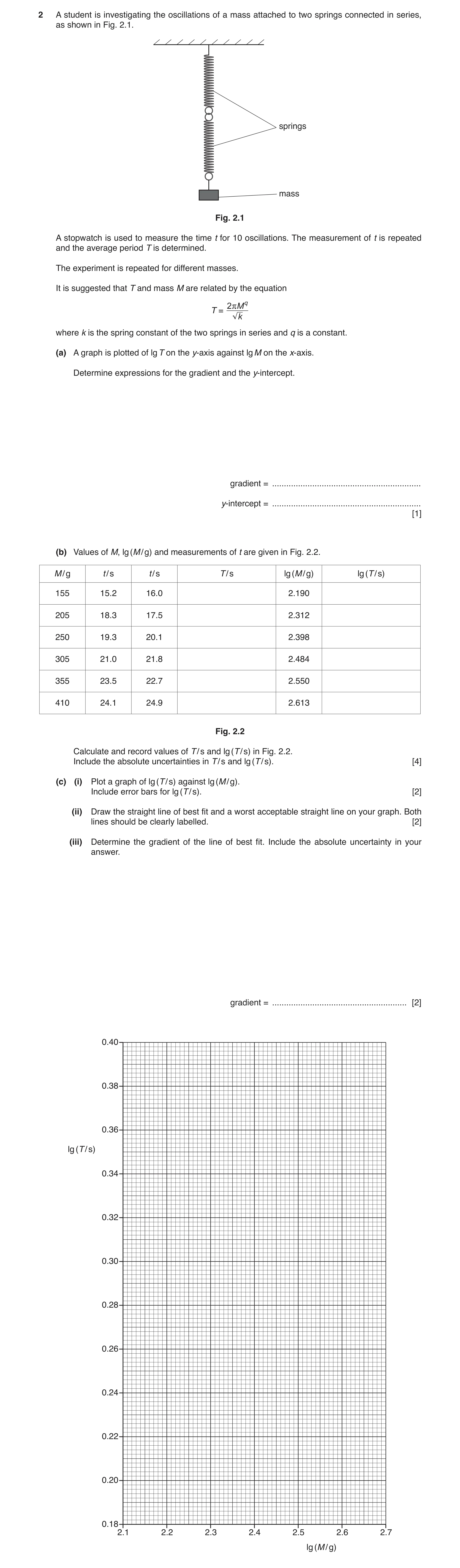
2 A student is investigating the oscillations of a mass attached to two springs connected in series, as shown in Fig. 2.1. springs mass Fig. 2.1 A stopwatch is used to measure the time t for 10 oscillations. The measurement of t is repeated and the average period T is determined. The experiment is repeated for different masses. It is suggested that T and mass M are related by the equation 2 r M q T = k where k is the spring constant of the two springs in series and q is a constant. (a) A graph is plotted of lg T on the y-axis against lg M on the x-axis. Determine expressions for the gradient and the y-intercept. gradient = … y-intercept = … [1] (b) Values of M, lg (M / g) and measurements of t are given in Fig. 2.2. M / g t / s t / s T / s lg (M / g) lg (T / s) 155 15.2 16.0 2.190 205 18.3 17.5 2.312 250 19.3 20.1 2.398 305 21.0 21.8 2.484 355 23.5 22.7 2.550 410 24.1 24.9 2.613 Fig. 2.2 Calculate and record values of T / s and lg (T / s) in Fig. 2.2. Include the absolute uncertainties in T / s and lg (T / s). [4] (c) (i) Plot a graph of lg (T / s) against lg (M / g). Include error bars for lg (T / s). [2] (ii) Draw the straight line of best fit and a worst acceptable straight line on your graph. Both lines should be clearly labelled. [2] (iii) Determine the gradient of the line of best fit. Include the absolute uncertainty in your answer. gradient = … [2]
11 marks
Mark scheme: 2(a) gradient = q and y-intercept = π = π − 2 1 lg lg 2 lg 2 k k 1 2(b) T / s lg (T / s) 1.56 0.193 or 0.1931 1.79 0.253 or 0.2529 1.97 0.294 or 0.2945 2.14 0.330 or 0.3304 2.31 0.364 or 0.3636 2.45 0.389 or 0.3892 Values of T as above. 1 Values of lg T as above. 1 Uncertainties in T all ±0.04. 1 Uncertainties in lg (T / s) consistent with uncertainties in T e.g. from ±0.011 to ±0.007. 1 Question Answer Marks 2(c)(i) Six points plotted correctly. Must be accurate to the nearest half a small square. Diameter of points must be less than half a small square. 1 Error bars in lg T plotted correctly. All error bars must be plotted. Length of bar must be accurate to less than half a small square and symmetrical. 1 2(c)(ii) Line of best fit drawn. Lower end of line should pass between (2.22, 0.22) and (2.25, 0.22) and upper end of line should pass between (2.49, 0.34) and (2.51, 0.34). Do not accept line from first to last plot. 1 Worst acceptable line drawn (steepest or shallowest possible line that passes through all the error bars). All error bars must be plotted. 1 2(c)(iii) Gradient determined with clear substitution of data points from the line of best fit into ∆y / ∆x. Distance between data points must be greater than half the length of the drawn line. 1 uncertainty = gradient of line of best fit – gradient of worst acceptable line or uncertainty = ½ (steepest worst line gradient – shallowest worst line gradient) 1 2(c)(iv) y-intercept determined by substitution of correct point from the line of best fit into y = mx + c. 1 2(d) k determined from y-intercept. 2 2 intercept 2 2 10 10 y k − π π = = (c)(iv) 1 q = answer to (c)(iii) and given to 2 or 3 significant figures. 1 Question Answer Marks 2(e) M determined from (d) or (c)(iii) and (c)(iv) with correct substitution shown. 2 2 2 2 4 q q q T k k k M = = = π π π or π − = 2 (lg1) lg lg k M q = − = − -intercept lg gradient y M (c)(iv) (c)(iii) 10 M − = (c)(iv) (c)(iii) 1
This question in 9702/51 Oct/Nov 2019
Q4 · When a light plastic ball is placed in a vertical column of moving air, the ball becomes… 9702/53 Oct/Nov 2019
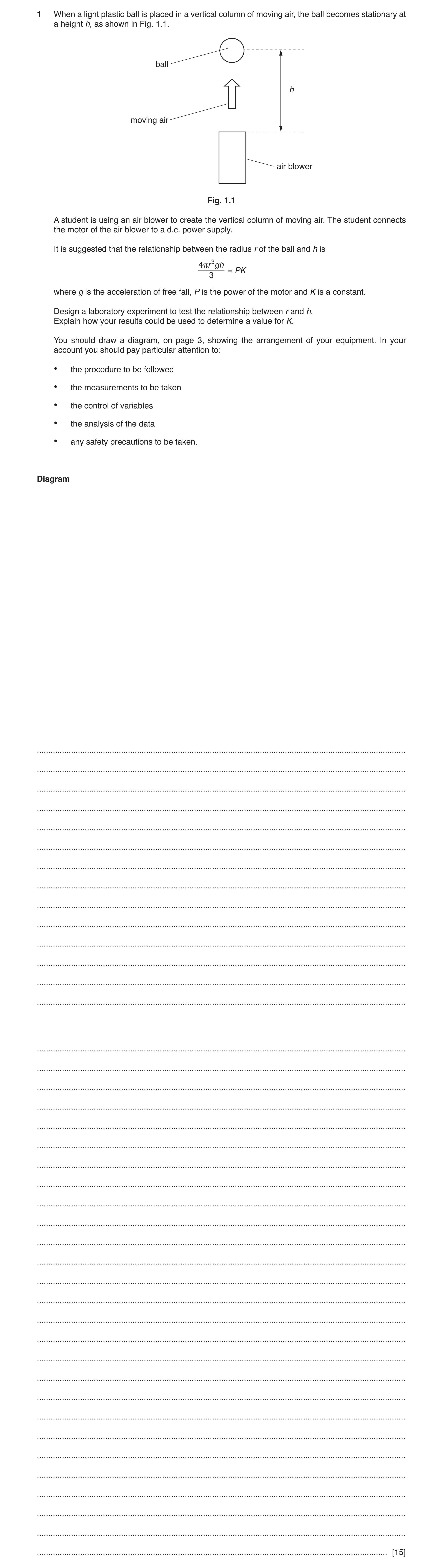
1 When a light plastic ball is placed in a vertical column of moving air, the ball becomes stationary at a height h, as shown in Fig. 1.1. ball h moving air air blower Fig. 1.1 A student is using an air blower to create the vertical column of moving air. The student connects the motor of the air blower to a d.c. power supply. It is suggested that the relationship between the radius r of the ball and h is 4 r r 3 gh = PK 3 where g is the acceleration of free fall, P is the power of the motor and K is a constant. Design a laboratory experiment to test the relationship between r and h. Explain how your results could be used to determine a value for K. You should draw a diagram, on page 3, showing the arrangement of your equipment. In your account you should pay particular attention to: • the procedure to be followed • the measurements to be taken • the control of variables • the analysis of the data • any safety precautions to be taken. Diagram … … … … … … … … … … … … … … … … … … … … … … … … … … … … … … … … … … … … … … … … … [15]
15 marks
Mark scheme: 1 Defining the problem r is the independent variable and h is the dependent variable or vary r and measure/determine h 1 keep P constant 1 Methods of data collection labelled diagram of workable experiment including: • labelled air blower • labelled ball vertically (by eye) above the blower • vertical (by eye) rule at least from top of blower to ball 1 circuit diagram to determine P, e.g. voltmeter and ammeter connected to motor and power supply or wattmeter connected to motor and power supply 1 use of micrometer/calipers/rule to measure diameter of ball 1 measure the distance between the top/middle/bottom of the ball and the top of the blower 1 Method of Analysis plot a graph of h against 1 / r3 (or lg h against lg r) 1 relationship valid if a straight line through (0,0) (for lg h against lg r straight line with gradient = –3) 1 4 gradient 3 g K P π × = (for lg h against lg r, intercept 4 10 3 y g K P − π × = ) 1 Question Answer Marks 1 Additional detail including safety considerations D1 use large box/tray to collect ball (to prevent ball rolling on floor/bouncing) or reasoned method to avoid draughts, e.g. switch off fans, close windows, use a screen 6 D2 method to determine P from correct circuit, e.g. P = I × V or use wattmeter to measure P D3 stand on bench with clamped rule vertically to measure vertical distance D4 method to ensure clamped rule to measure h is vertical, e.g. correctly positioned set square indicated at right angles between the rule and the horizontal surface or plumb line shown in appropriate position D5 r = d / 2 when diameter measured D6 repeat diameter measurement in different directions and find average D7 repeat experiment for each value of r and determine average h D8 method to determine h, e.g. h = reading top of ball – r – top of blower or h = reading bottom of ball + r – top of blower or h = (distance from top of ball to top of blower + distance from bottom of ball to top of blower) / 2 D9 wait for the ball to become stationary (vertically) D10 video (camera) shown level with elevated ball and description of playback frame-by-frame or slow motion
This question in 9702/53 Oct/Nov 2019
Q5 · A student is investigating the oscillations of a mass attached to two springs connected… 9702/53 Oct/Nov 2019
2 A student is investigating the oscillations of a mass attached to two springs connected in series, as shown in Fig. 2.1. springs mass Fig. 2.1 A stopwatch is used to measure the time t for 10 oscillations. The measurement of t is repeated and the average period T is determined. The experiment is repeated for different masses. It is suggested that T and mass M are related by the equation 2 r M q T = k where k is the spring constant of the two springs in series and q is a constant. (a) A graph is plotted of lg T on the y-axis against lg M on the x-axis. Determine expressions for the gradient and the y-intercept. gradient = … y-intercept = … [1] (b) Values of M, lg (M / g) and measurements of t are given in Fig. 2.2. M / g t / s t / s T / s lg (M / g) lg (T / s) 155 15.2 16.0 2.190 205 18.3 17.5 2.312 250 19.3 20.1 2.398 305 21.0 21.8 2.484 355 23.5 22.7 2.550 410 24.1 24.9 2.613 Fig. 2.2 Calculate and record values of T / s and lg (T / s) in Fig. 2.2. Include the absolute uncertainties in T / s and lg (T / s). [4] (c) (i) Plot a graph of lg (T / s) against lg (M / g). Include error bars for lg (T / s). [2] (ii) Draw the straight line of best fit and a worst acceptable straight line on your graph. Both lines should be clearly labelled. [2] (iii) Determine the gradient of the line of best fit. Include the absolute uncertainty in your answer. gradient = … [2]
11 marks
Mark scheme: 2(a) gradient = q and y-intercept = π = π − 2 1 lg lg 2 lg 2 k k 1 2(b) T / s lg (T / s) 1.56 0.193 or 0.1931 1.79 0.253 or 0.2529 1.97 0.294 or 0.2945 2.14 0.330 or 0.3304 2.31 0.364 or 0.3636 2.45 0.389 or 0.3892 Values of T as above. 1 Values of lg T as above. 1 Uncertainties in T all ±0.04. 1 Uncertainties in lg (T / s) consistent with uncertainties in T e.g. from ±0.011 to ±0.007. 1 Question Answer Marks 2(c)(i) Six points plotted correctly. Must be accurate to the nearest half a small square. Diameter of points must be less than half a small square. 1 Error bars in lg T plotted correctly. All error bars must be plotted. Length of bar must be accurate to less than half a small square and symmetrical. 1 2(c)(ii) Line of best fit drawn. Lower end of line should pass between (2.22, 0.22) and (2.25, 0.22) and upper end of line should pass between (2.49, 0.34) and (2.51, 0.34). Do not accept line from first to last plot. 1 Worst acceptable line drawn (steepest or shallowest possible line that passes through all the error bars). All error bars must be plotted. 1 2(c)(iii) Gradient determined with clear substitution of data points from the line of best fit into ∆y / ∆x. Distance between data points must be greater than half the length of the drawn line. 1 uncertainty = gradient of line of best fit – gradient of worst acceptable line or uncertainty = ½ (steepest worst line gradient – shallowest worst line gradient) 1 2(c)(iv) y-intercept determined by substitution of correct point from the line of best fit into y = mx + c. 1 2(d) k determined from y-intercept. 2 2 intercept 2 2 10 10 y k − π π = = (c)(iv) 1 q = answer to (c)(iii) and given to 2 or 3 significant figures. 1 Question Answer Marks 2(e) M determined from (d) or (c)(iii) and (c)(iv) with correct substitution shown. 2 2 2 2 4 q q q T k k k M = = = π π π or π − = 2 (lg1) lg lg k M q = − = − -intercept lg gradient y M (c)(iv) (c)(iii) 10 M − = (c)(iv) (c)(iii) 1
This question in 9702/53 Oct/Nov 2019
Q6 · A student investigates springs made of metal wire, as shown in Fig 9702/51 May/June 2020
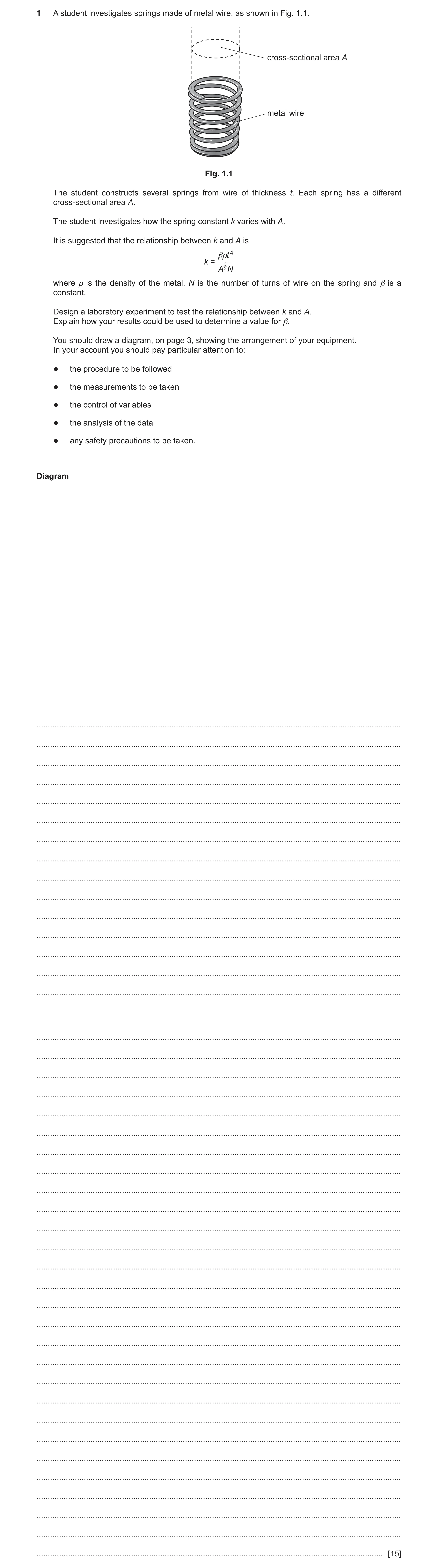
1 A student investigates springs made of metal wire, as shown in Fig. 1.1. cross-sectional area A metal wire Fig. 1.1 The student constructs several springs from wire of thickness t. Each spring has a different cross-sectional area A. The student investigates how the spring constant k varies with A. It is suggested that the relationship between k and A is βρt 4 k = 3 A 2N where ρ is the density of the metal, N is the number of turns of wire on the spring and β is a constant. Design a laboratory experiment to test the relationship between k and A. Explain how your results could be used to determine a value for β. You should draw a diagram, on page 3, showing the arrangement of your equipment. In your account you should pay particular attention to: ● the procedure to be followed ● the measurements to be taken ● the control of variables ● the analysis of the data ● any safety precautions to be taken. Diagram … … … … … … … … … … … … … … … … … … … … … … … … … … … … … … … … … … … … … … … … … … … [15]
15 marks
Mark scheme: 1 Defining the problem A is the independent variable and k is the dependent variable or vary A and measure k 1 keep N constant 1 Methods of data collection labelled diagram of workable experiment including: • spring fixed at one end to a support • load attached to the other end of the spring • labelled load 1 method to measure mass or weight of load: use top-pan balance to measure mass or newton meter to measure weight 1 use of a micrometer/calipers to determine t and rule/calipers to measure the diameter of the spring 1 method to measure extension, e.g. labelled ruler drawn parallel to spring, equilibrium position and displaced position indicated and x indicated or description of use of ruler to measure equilibrium position and displaced position and difference determined 1 Method of analysis plot a graph of k against 1 / A3/2 (or A–3/2) or equivalent e.g. lg k against lg A 1 relationship valid if a straight line passing through the origin is produced (for lg k against lg A, relationship valid if a straight line with gradient –3/2) 1 4 gradient N t β ρ × = [for lg k against lg A, β = 10y-intercept × N / (ρt4) ] 1 Question Answer Marks 1 Additional detail including safety considerations 6 D1 use safety goggles/safety screen to prevent injury to eyes from (moving) spring/load or use cushion/sand box in case load falls D2 keep t constant D3 or mg F k x x = D4 use of set square when taking measurements to determine extension of spring D5 repeat measurement of t along wire/spring and average D6 repeat measurement of diameter D of spring (to determine A) in different directions and average D7 use of 2 4 D A π = D8 method to ensure clamped rule to measure extension is vertical, e.g. correctly positioned set square indicated at right angles between the rule and the horizontal surface or plumb line shown in appropriate position D9 method to determine the density of the wire or additional detail on construction of coil D10 method to determine the mean diameter of the spring, e.g. subtract t from external diameter of spring Question Answer Marks
This question in 9702/51 May/June 2020
Q7 · A student investigates springs made of metal wire, as shown in Fig 9702/53 May/June 2020
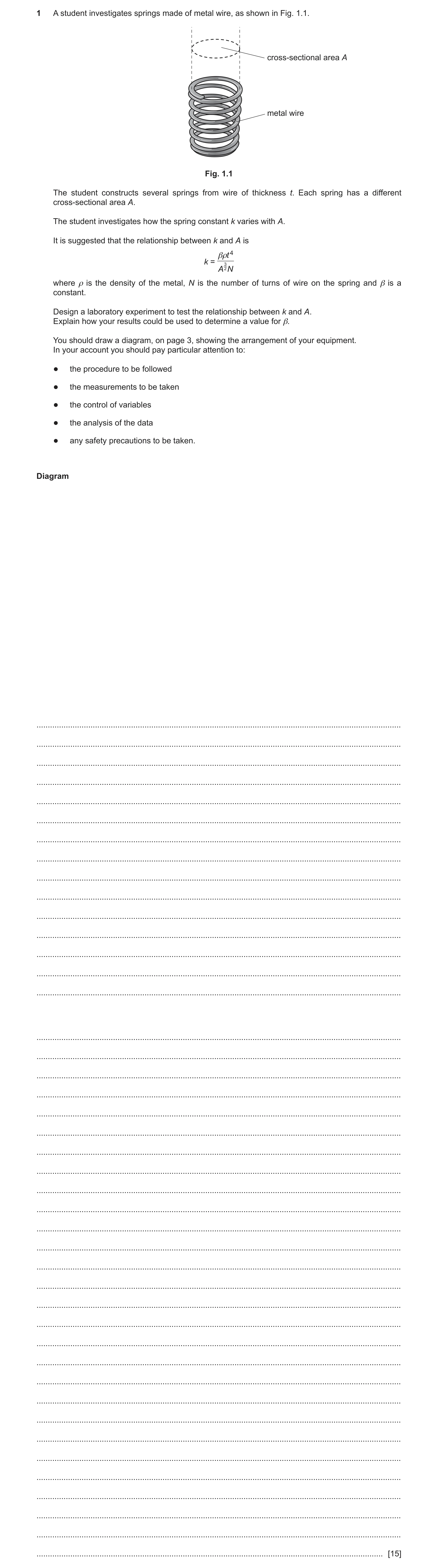
1 A student investigates springs made of metal wire, as shown in Fig. 1.1. cross-sectional area A metal wire Fig. 1.1 The student constructs several springs from wire of thickness t. Each spring has a different cross-sectional area A. The student investigates how the spring constant k varies with A. It is suggested that the relationship between k and A is βρt 4 k = 3 A 2N where ρ is the density of the metal, N is the number of turns of wire on the spring and β is a constant. Design a laboratory experiment to test the relationship between k and A. Explain how your results could be used to determine a value for β. You should draw a diagram, on page 3, showing the arrangement of your equipment. In your account you should pay particular attention to: ● the procedure to be followed ● the measurements to be taken ● the control of variables ● the analysis of the data ● any safety precautions to be taken. Diagram … … … … … … … … … … … … … … … … … … … … … … … … … … … … … … … … … … … … … … … … … … … [15]
15 marks
Mark scheme: 1 Defining the problem A is the independent variable and k is the dependent variable or vary A and measure k 1 keep N constant 1 Methods of data collection labelled diagram of workable experiment including: • spring fixed at one end to a support • load attached to the other end of the spring • labelled load 1 method to measure mass or weight of load: use top-pan balance to measure mass or newton meter to measure weight 1 use of a micrometer/calipers to determine t and rule/calipers to measure the diameter of the spring 1 method to measure extension, e.g. labelled ruler drawn parallel to spring, equilibrium position and displaced position indicated and x indicated or description of use of ruler to measure equilibrium position and displaced position and difference determined 1 Method of analysis plot a graph of k against 1 / A3/2 (or A–3/2) or equivalent e.g. lg k against lg A 1 relationship valid if a straight line passing through the origin is produced (for lg k against lg A, relationship valid if a straight line with gradient –3/2) 1 4 gradient N t β ρ × = [for lg k against lg A, β = 10y-intercept × N / (ρt4) ] 1 Question Answer Marks 1 Additional detail including safety considerations 6 D1 use safety goggles/safety screen to prevent injury to eyes from (moving) spring/load or use cushion/sand box in case load falls D2 keep t constant D3 or mg F k x x = D4 use of set square when taking measurements to determine extension of spring D5 repeat measurement of t along wire/spring and average D6 repeat measurement of diameter D of spring (to determine A) in different directions and average D7 use of 2 4 D A π = D8 method to ensure clamped rule to measure extension is vertical, e.g. correctly positioned set square indicated at right angles between the rule and the horizontal surface or plumb line shown in appropriate position D9 method to determine the density of the wire or additional detail on construction of coil D10 method to determine the mean diameter of the spring, e.g. subtract t from external diameter of spring Question Answer Marks
This question in 9702/53 May/June 2020
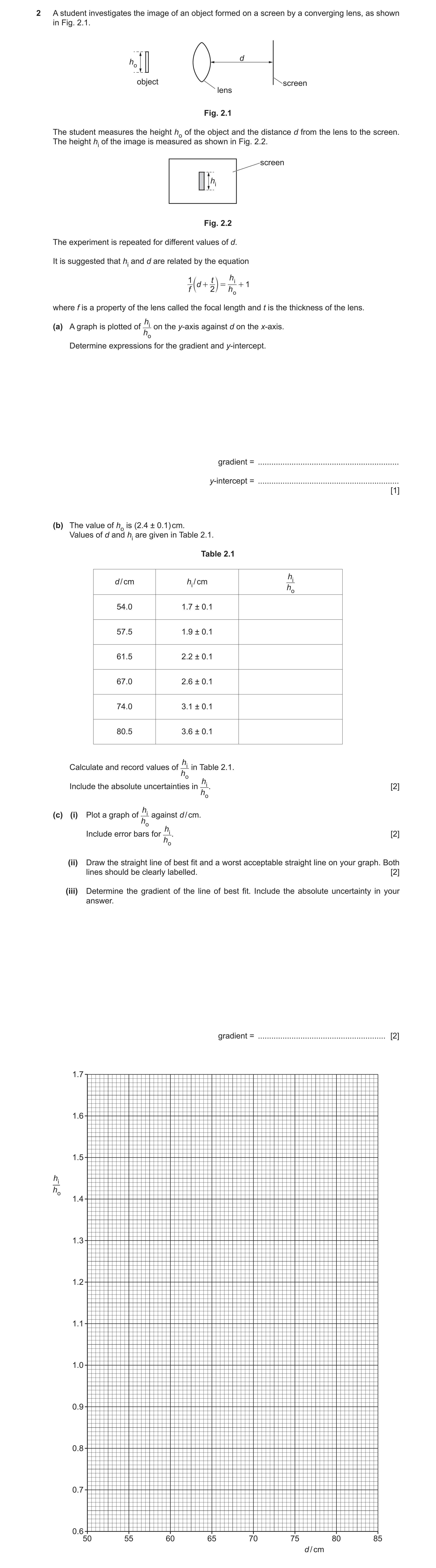
Q8 · A student investigates the image of an object formed on a screen by a converging lens, as… 9702/51 Oct/Nov 2020
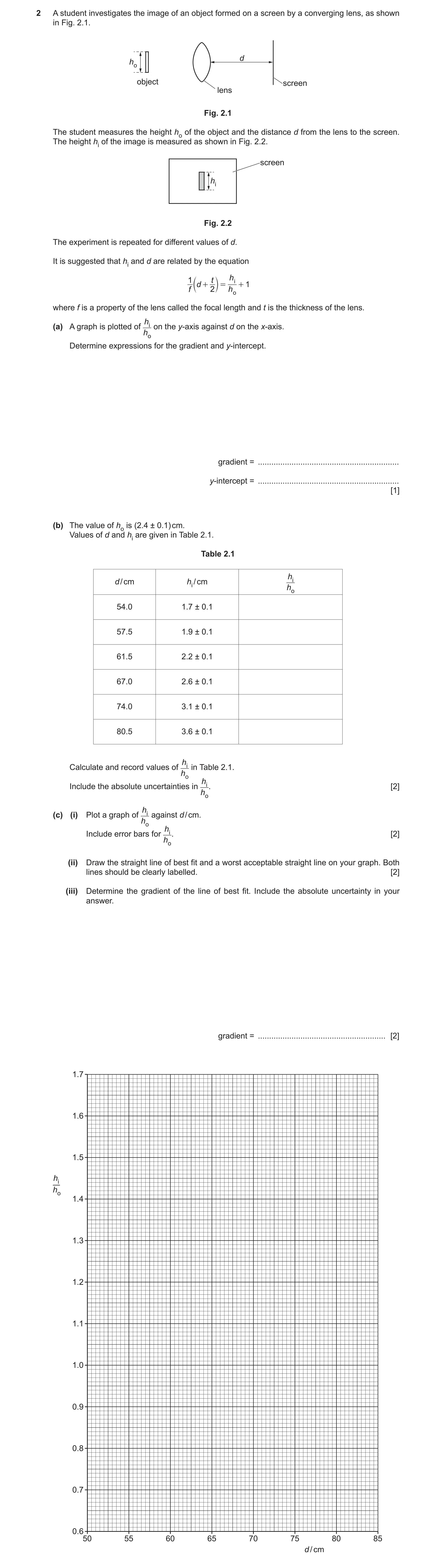
2 A student investigates the image of an object formed on a screen by a converging lens, as shown in Fig. 2.1. d ho object screen lens Fig. 2.1 The student measures the height ho of the object and the distance d from the lens to the screen. The height hi of the image is measured as shown in Fig. 2.2. screen hi Fig. 2.2 The experiment is repeated for different values of d. It is suggested that hi and d are related by the equation 1 t h i d + = + 1 f c 2 m h o where f is a property of the lens called the focal length and t is the thickness of the lens. hi (a) A graph is plotted of on the y-axis against d on the x-axis. ho Determine expressions for the gradient and y-intercept. gradient = … y-intercept = … [1] (b) The value of ho is (2.4 ± 0.1) cm. Values of d and hi are given in Table 2.1. Table 2.1 hi d / cm hi / cm ho 54.0 1.7 ± 0.1 57.5 1.9 ± 0.1 61.5 2.2 ± 0.1 67.0 2.6 ± 0.1 74.0 3.1 ± 0.1 80.5 3.6 ± 0.1 hi Calculate and record values of in Table 2.1. ho hi Include the absolute uncertainties in . [2] ho hi(c) (i) Plot a graph of against d / cm. ho hi Include error bars for . [2] ho (ii) Draw the straight line of best fit and a worst acceptable straight line on your graph. Both lines should be clearly labelled. [2] (iii) Determine the gradient of the line of best fit. Include the absolute uncertainty in your answer. gradient = … [2]
9 marks
Mark scheme: 2(a) gradient = 1 f y-intercept = 1 2 t f − 1 2(b) i o h h 0.71 or 0.708 0.79 or 0.792 0.92 or 0.917 1.1 or 1.08 1.3 or 1.29 1.5 or 1.50 1 Absolute uncertainties in i o h h from ± 0.07 to ± 0.1 (or ± 0.10 or ± 0.11). 1 2(c)(i) Six points plotted correctly. Must be accurate to nearest half a small square. Diameter of points must be less than half a small square. 1 Error bars in i o h h plotted correctly. All error bars must be plotted. Total length of bar must be accurate to less than half a small square and symmetrical. 1 Question Answer Marks 2(c)(ii) Line of best fit drawn. Points must be balanced. Do not accept line from top to bottom point. Line must pass between (55, 0.75) and (56, 0.75) and between (77, 1.40) and (78, 1.40). 1 Worst acceptable line drawn (steepest or shallowest possible line that passes through all the error bars). All error bars must be plotted. 1 2(c)(iii) Gradient determined with clear substitution of data points into Δy / Δx. Distance between data points must be at least half the length of the drawn line. 1 Gradient of worst acceptable line determined. uncertainty = (gradient of line of best fit – gradient of worst acceptable line) or uncertainty = ½ (steepest worst line gradient – shallowest worst line gradient) 1 2(c)(iv) y-intercept determined from substitution into y = mx + c. 1 y-intercept determined using gradient from worst acceptable line. uncertainty = y-intercept of line of best fit – y-intercept of worst acceptable line or uncertainty = ½ (steepest worst line y-intercept – shallowest worst line y-intercept) No ECF from false origin method. 1 Question Answer Marks 2(d)(i) f determined using gradient with correct substitution shown. = = 1 1 gradient f (c)(iii) 1 f determined using gradient and given to two or three significant figures and correct SI unit shown with correct power of ten e.g. 33 cm or 0.33 m or 33.1 cm or 0.331 m 1 Absolute uncertainty in f determined. Δ = × gradient absolute uncertainty in gradient f f 1 2(d)(ii) t determined using y-intercept and given to two or three significant figures. Correct substitution of numbers required. ( ) 2 -intercept 1 t f y = × + or ( ) × + = 2 -intercept 1 gradient y t 1
This question in 9702/51 Oct/Nov 2020
Q9 · A student investigates the image of an object formed on a screen by a converging lens, as… 9702/53 Oct/Nov 2020
2 A student investigates the image of an object formed on a screen by a converging lens, as shown in Fig. 2.1. d ho object screen lens Fig. 2.1 The student measures the height ho of the object and the distance d from the lens to the screen. The height hi of the image is measured as shown in Fig. 2.2. screen hi Fig. 2.2 The experiment is repeated for different values of d. It is suggested that hi and d are related by the equation 1 t h i d + = + 1 f c 2 m h o where f is a property of the lens called the focal length and t is the thickness of the lens. hi (a) A graph is plotted of on the y-axis against d on the x-axis. ho Determine expressions for the gradient and y-intercept. gradient = … y-intercept = … [1] (b) The value of ho is (2.4 ± 0.1) cm. Values of d and hi are given in Table 2.1. Table 2.1 hi d / cm hi / cm ho 54.0 1.7 ± 0.1 57.5 1.9 ± 0.1 61.5 2.2 ± 0.1 67.0 2.6 ± 0.1 74.0 3.1 ± 0.1 80.5 3.6 ± 0.1 hi Calculate and record values of in Table 2.1. ho hi Include the absolute uncertainties in . [2] ho hi(c) (i) Plot a graph of against d / cm. ho hi Include error bars for . [2] ho (ii) Draw the straight line of best fit and a worst acceptable straight line on your graph. Both lines should be clearly labelled. [2] (iii) Determine the gradient of the line of best fit. Include the absolute uncertainty in your answer. gradient = … [2]
9 marks
Mark scheme: 2(a) gradient = 1 f y-intercept = 1 2 t f − 1 2(b) i o h h 0.71 or 0.708 0.79 or 0.792 0.92 or 0.917 1.1 or 1.08 1.3 or 1.29 1.5 or 1.50 1 Absolute uncertainties in i o h h from ± 0.07 to ± 0.1 (or ± 0.10 or ± 0.11). 1 2(c)(i) Six points plotted correctly. Must be accurate to nearest half a small square. Diameter of points must be less than half a small square. 1 Error bars in i o h h plotted correctly. All error bars must be plotted. Total length of bar must be accurate to less than half a small square and symmetrical. 1 Question Answer Marks 2(c)(ii) Line of best fit drawn. Points must be balanced. Do not accept line from top to bottom point. Line must pass between (55, 0.75) and (56, 0.75) and between (77, 1.40) and (78, 1.40). 1 Worst acceptable line drawn (steepest or shallowest possible line that passes through all the error bars). All error bars must be plotted. 1 2(c)(iii) Gradient determined with clear substitution of data points into Δy / Δx. Distance between data points must be at least half the length of the drawn line. 1 Gradient of worst acceptable line determined. uncertainty = (gradient of line of best fit – gradient of worst acceptable line) or uncertainty = ½ (steepest worst line gradient – shallowest worst line gradient) 1 2(c)(iv) y-intercept determined from substitution into y = mx + c. 1 y-intercept determined using gradient from worst acceptable line. uncertainty = y-intercept of line of best fit – y-intercept of worst acceptable line or uncertainty = ½ (steepest worst line y-intercept – shallowest worst line y-intercept) No ECF from false origin method. 1 Question Answer Marks 2(d)(i) f determined using gradient with correct substitution shown. = = 1 1 gradient f (c)(iii) 1 f determined using gradient and given to two or three significant figures and correct SI unit shown with correct power of ten e.g. 33 cm or 0.33 m or 33.1 cm or 0.331 m 1 Absolute uncertainty in f determined. Δ = × gradient absolute uncertainty in gradient f f 1 2(d)(ii) t determined using y-intercept and given to two or three significant figures. Correct substitution of numbers required. ( ) 2 -intercept 1 t f y = × + or ( ) × + = 2 -intercept 1 gradient y t 1
This question in 9702/53 Oct/Nov 2020
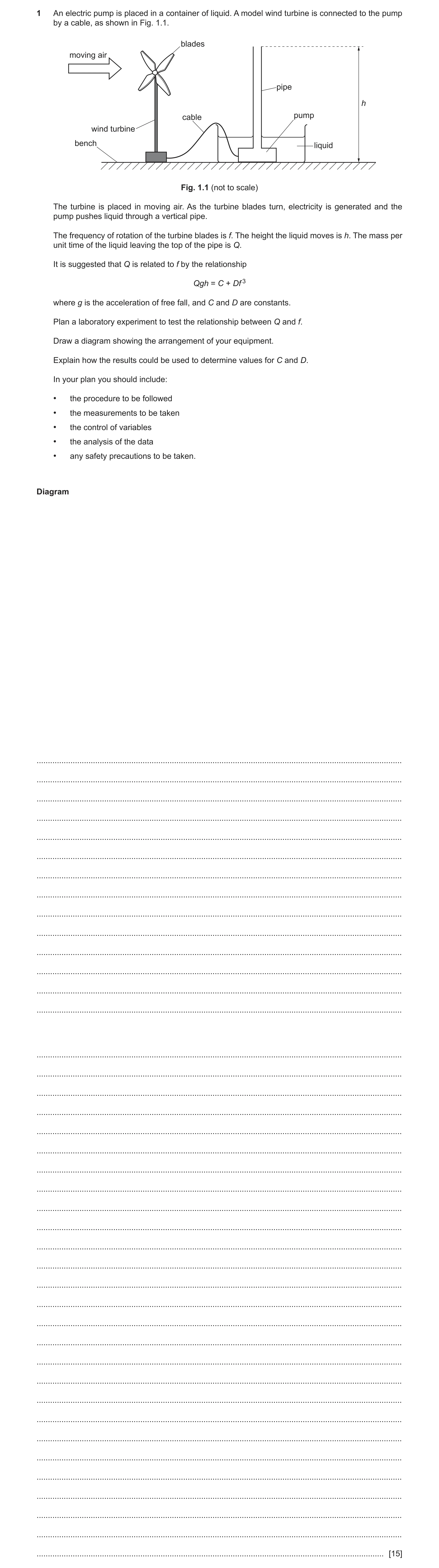
Q10 · An electric pump is placed in a container of liquid 9702/52 Feb/March 2023
1 An electric pump is placed in a container of liquid. A model wind turbine is connected to the pump by a cable, as shown in Fig. 1.1. blades moving air pipe h cable pump wind turbine bench liquid Fig. 1.1 (not to scale) The turbine is placed in moving air. As the turbine blades turn, electricity is generated and the pump pushes liquid through a vertical pipe. The frequency of rotation of the turbine blades is f. The height the liquid moves is h. The mass per unit time of the liquid leaving the top of the pipe is Q. It is suggested that Q is related to f by the relationship Qgh = C + Df 3 where g is the acceleration of free fall, and C and D are constants. Plan a laboratory experiment to test the relationship between Q and f. Draw a diagram showing the arrangement of your equipment. Explain how the results could be used to determine values for C and D. In your plan you should include: • the procedure to be followed • the measurements to be taken • the control of variables • the analysis of the data • any safety precautions to be taken. Diagram … … … … … … … … … … … … … … … … … … … … … … … … … … … … … … … … … … … … … … … … … [15]
15 marks
Mark scheme: Question Answer Marks 1 Defining the problem f is the independent variable and Q is the dependent variable, or vary f and measure Q. 1 Keep h constant 1 Methods of data collection Labelled diagram of workable experiment including: 1 • fan is positioned in line with the turbine so that blades of both fan and turbine overlap • base of fan on same bench as turbine • fan labelled and one other label from bench, (wind) turbine, cable, pump, pipe, liquid Labelled apparatus showing workable method to collect the liquid from the top of the pipe, e.g. hose / pipe / tube connected 1 to top of pipe with the other end over a beaker / measuring cylinder below top of pipe. At least one label related to collection of liquid. Use of stop-watch / timer to measure time to collect liquid or to measure time for blades to rotate. 1 Use of (top pan) balance to measure mass of liquid leaving the pipe. 1 Method of Analysis Plots a graph of Q against f 3 or equivalent (e.g. f 3 against Q). 1 Do not accept logarithmic graphs. C = gh -intercepty (for f 3 against Q: C = −D -intercepty ) 1 D = gh gradient 1 3 gh (for f against Q: D = ) gradient 1 Additional detail including safety considerations 6 Any six from: D1 Precaution with reason linked to prevent liquid spilling (on bench / floor) e.g. use of large bucket / bowl / tray to contain any spilled liquid or Precaution with reason linked to prevent air / dust particles in eye, e.g. use of goggles or Precaution with reason linked to turbine falling, e.g. clamp turbine to bench. D2 Use rule to measure h. D3 Method to determine mass of liquid, e.g. mass of beaker + liquid – mass of empty beaker or mass of container / pipe before – mass of container / pipe after. D4 Method to determine f, e.g. measure time t for many rotations / revolutions N and period T = t /N and f = 1/T or measure time t for many rotations / revolutions N and f = N/t or video rotating blades, playback frame by frame and use a time stamp to determine period T and f = 1/T. D5 Mark one of the blades to assist in counting number of rotations. D6 Method to vary f, e.g. change speed of fan / change distance between fan and blades / vary current in fan. D7 Wait for steady air flow before starting timing and / or collecting liquid. mass (of liquid) D8 Q = time (to collect liquid) or method and explanation to reduce uncertainty in Q, e.g. use large value of time or mass of liquid collected. D9 Repeat measurements of Q for the same value of f and average Q. 1 D10 Relationship valid if a straight line is produced (not passing through the origin). Do not accept passing through the origin.
This question in 9702/52 Feb/March 2023
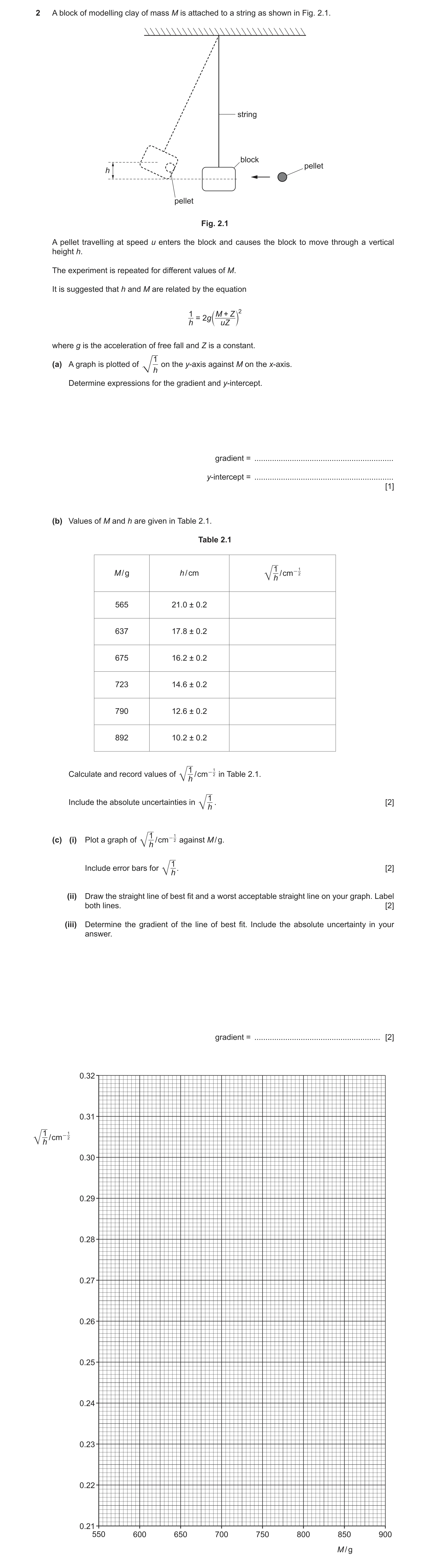
Q11 · A block of modelling clay of mass M is attached to a string as shown in Fig 9702/51 Oct/Nov 2023
2 A block of modelling clay of mass M is attached to a string as shown in Fig. 2.1. string block pellet h pellet Fig. 2.1 A pellet travelling at speed u enters the block and causes the block to move through a vertical height h. The experiment is repeated for different values of M. It is suggested that h and M are related by the equation 1 M + Z 2 = 2 g h c uZ m where g is the acceleration of free fall and Z is a constant. 1 (a) A graph is plotted of on the y-axis against M on the x-axis. h Determine expressions for the gradient and y-intercept. gradient = … y-intercept = … [1] (b) Values of M and h are given in Table 2.1. Table 2.1 1 1 - M / g h / cm / cm 2 h 565 21.0 ± 0.2 637 17.8 ± 0.2 675 16.2 ± 0.2 723 14.6 ± 0.2 790 12.6 ± 0.2 892 10.2 ± 0.2 1 1 - Calculate and record values of / cm 2 in Table 2.1. h 1 Include the absolute uncertainties in . [2] h 1 1 - 2 against M / g.(c) (i) Plot a graph of / cm h 1 Include error bars for . [2] h (ii) Draw the straight line of best fit and a worst acceptable straight line on your graph. Label both lines. [2] (iii) Determine the gradient of the line of best fit. Include the absolute uncertainty in your answer. gradient = … [2]
9 marks
Mark scheme: 2(a) 2g 1 gradient = uZ 2g y-intercept = u 2(b) 1 −1 1 2 / cm h 0.218 or 0.2182 0.237 or 0.2370 0.248 or 0.2485 0.262 or 0.2617 0.282 or 0.2817 0.313 or 0.3131 Values correct as shown above. 1 1 Uncertainties in from ± 0.001 to ± 0.003. h 2(c)(i) Six points from (b) plotted correctly. 1 Must be within half a small square. Diameter of points must be less than half a small square. 1 1 Error bars in plotted correctly. h All error bars to be plotted. Total length of bar must be accurate to less than half a small square and symmetrical. 2(c)(ii) Straight line of best fit drawn. 1 Do not accept line from top point to bottom point. Points must be balanced. Line must pass between (605, 0.230) and (615, 0.230) and between (845, 0.300) and (855, 0.300) Worst acceptable line drawn (steepest or shallowest possible line that passes through all the error bars). 1 All error bars must be plotted. 2(c)(iii) Gradient determined with clear substitution of data points into y / x. 1 Distance between data points must be greater than half the length of the drawn line. Gradient determined of worst acceptable line. 1 uncertainty = (gradient of line of best fit – gradient of worst acceptable line) or uncertainty = ½ (steepest worst line gradient – shallowest worst line gradient) 2(c)(iv) y-intercept determined by substitution of correct point with consistent power of ten into y = mx + c. 1 y-intercept of worst acceptable line determined by substitution into y = mx + c. 1 uncertainty = y-intercept of line of best fit – y-intercept of worst acceptable line or uncertainty = ½ (steepest worst line y-intercept – shallowest worst line y-intercept) Do not accept ECF from false origin method. 2(d)(i) u determined using y-intercept and u and Z given to 2, 3 or 4 significant figures. 1 2 981 44.29 u = = y -intercept (c)(iv) Z determined using gradient with method shown and u and Z given with SI units with appropriate powers of ten. 1 2 981 44.29 y -intercept (c)(iv) Z = = or Z = = u gradient u (c)(iii) gradient (c)(iii) 2(d)(ii) Percentage uncertainty in Z with method shown. 1 y -intercept gradient percentage uncertainty in Z = + 100 y -intercept gradient or Correct substitution for u and u gradient percentage uncertainty in Z = + 100 u gradient or Correct substitution for max/min methods. 2(e) M determined to a minimum of 2 significant figures from (c)(iii) and (c)(iv) or (d)(i) with correct substitution. 1 1 − y -intercept 25 M = gradient or uZ uZ M = − Z = − Z 2gh 221.5
This question in 9702/51 Oct/Nov 2023
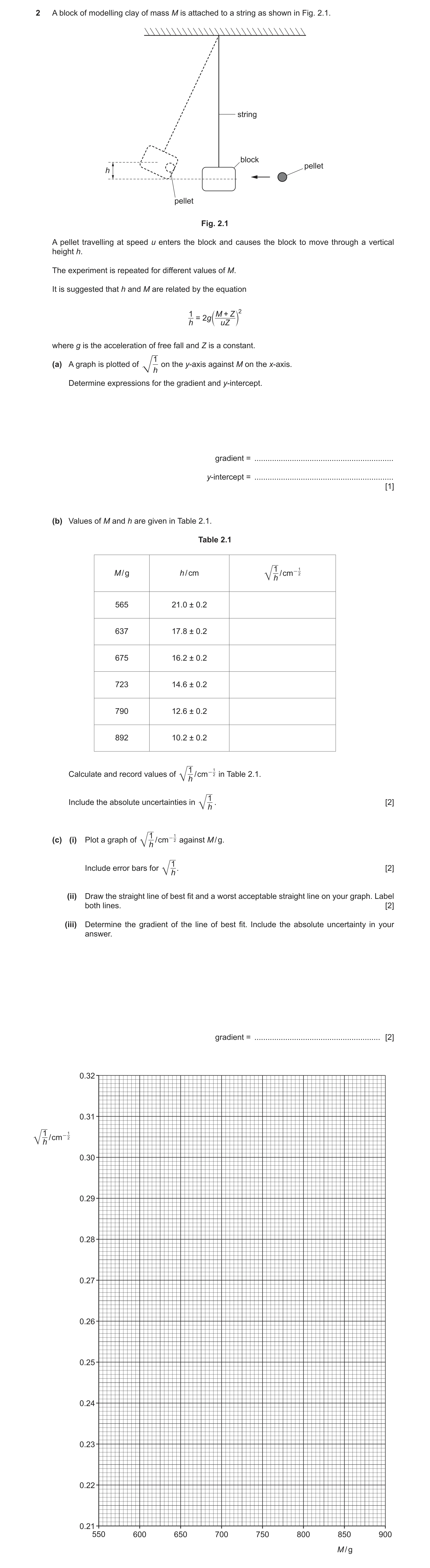
Q12 · A block of modelling clay of mass M is attached to a string as shown in Fig 9702/53 Oct/Nov 2023
2 A block of modelling clay of mass M is attached to a string as shown in Fig. 2.1. string block pellet h pellet Fig. 2.1 A pellet travelling at speed u enters the block and causes the block to move through a vertical height h. The experiment is repeated for different values of M. It is suggested that h and M are related by the equation 1 M + Z 2 = 2 g h c uZ m where g is the acceleration of free fall and Z is a constant. 1 (a) A graph is plotted of on the y-axis against M on the x-axis. h Determine expressions for the gradient and y-intercept. gradient = … y-intercept = … [1] (b) Values of M and h are given in Table 2.1. Table 2.1 1 1 - M / g h / cm / cm 2 h 565 21.0 ± 0.2 637 17.8 ± 0.2 675 16.2 ± 0.2 723 14.6 ± 0.2 790 12.6 ± 0.2 892 10.2 ± 0.2 1 1 - Calculate and record values of / cm 2 in Table 2.1. h 1 Include the absolute uncertainties in . [2] h 1 1 - 2 against M / g.(c) (i) Plot a graph of / cm h 1 Include error bars for . [2] h (ii) Draw the straight line of best fit and a worst acceptable straight line on your graph. Label both lines. [2] (iii) Determine the gradient of the line of best fit. Include the absolute uncertainty in your answer. gradient = … [2]
9 marks
Mark scheme: 2(a) 2g 1 gradient = uZ 2g y-intercept = u 2(b) 1 −1 1 2 / cm h 0.218 or 0.2182 0.237 or 0.2370 0.248 or 0.2485 0.262 or 0.2617 0.282 or 0.2817 0.313 or 0.3131 Values correct as shown above. 1 1 Uncertainties in from ± 0.001 to ± 0.003. h 2(c)(i) Six points from (b) plotted correctly. 1 Must be within half a small square. Diameter of points must be less than half a small square. 1 1 Error bars in plotted correctly. h All error bars to be plotted. Total length of bar must be accurate to less than half a small square and symmetrical. 2(c)(ii) Straight line of best fit drawn. 1 Do not accept line from top point to bottom point. Points must be balanced. Line must pass between (605, 0.230) and (615, 0.230) and between (845, 0.300) and (855, 0.300) Worst acceptable line drawn (steepest or shallowest possible line that passes through all the error bars). 1 All error bars must be plotted. 2(c)(iii) Gradient determined with clear substitution of data points into y / x. 1 Distance between data points must be greater than half the length of the drawn line. Gradient determined of worst acceptable line. 1 uncertainty = (gradient of line of best fit – gradient of worst acceptable line) or uncertainty = ½ (steepest worst line gradient – shallowest worst line gradient) 2(c)(iv) y-intercept determined by substitution of correct point with consistent power of ten into y = mx + c. 1 y-intercept of worst acceptable line determined by substitution into y = mx + c. 1 uncertainty = y-intercept of line of best fit – y-intercept of worst acceptable line or uncertainty = ½ (steepest worst line y-intercept – shallowest worst line y-intercept) Do not accept ECF from false origin method. 2(d)(i) u determined using y-intercept and u and Z given to 2, 3 or 4 significant figures. 1 2 981 44.29 u = = y -intercept (c)(iv) Z determined using gradient with method shown and u and Z given with SI units with appropriate powers of ten. 1 2 981 44.29 y -intercept (c)(iv) Z = = or Z = = u gradient u (c)(iii) gradient (c)(iii) 2(d)(ii) Percentage uncertainty in Z with method shown. 1 y -intercept gradient percentage uncertainty in Z = + 100 y -intercept gradient or Correct substitution for u and u gradient percentage uncertainty in Z = + 100 u gradient or Correct substitution for max/min methods. 2(e) M determined to a minimum of 2 significant figures from (c)(iii) and (c)(iv) or (d)(i) with correct substitution. 1 1 − y -intercept 25 M = gradient or uZ uZ M = − Z = − Z 2gh 221.5
This question in 9702/53 Oct/Nov 2023
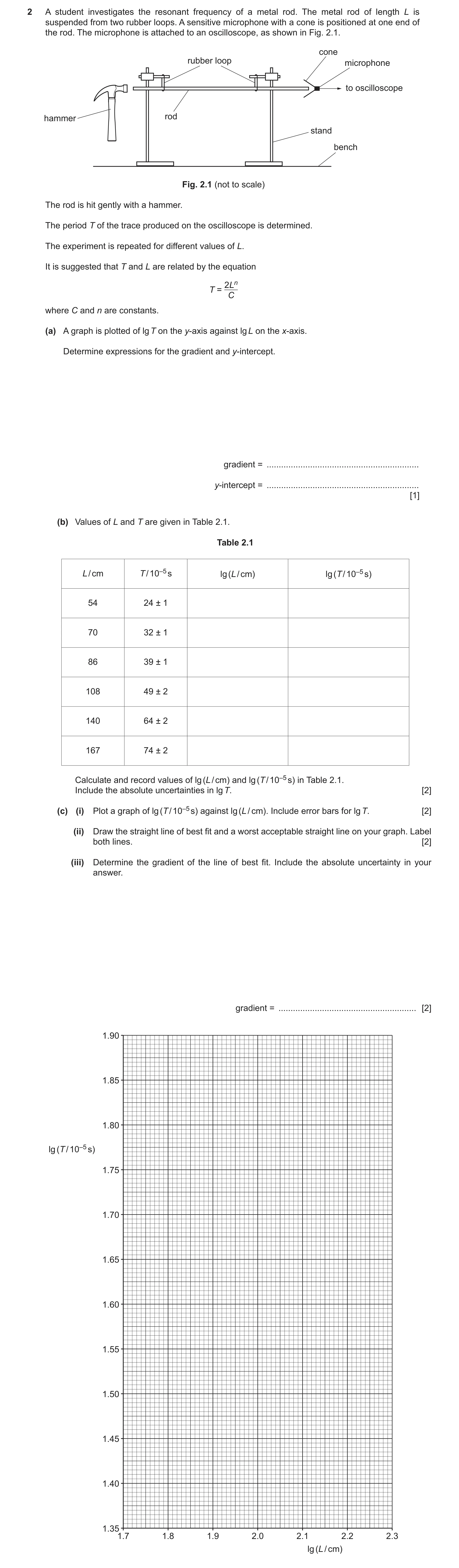
Q13 · A student investigates the resonant frequency of a metal rod 9702/52 May/June 2024
2 A student investigates the resonant frequency of a metal rod. The metal rod of length L is suspended from two rubber loops. A sensitive microphone with a cone is positioned at one end of the rod. The microphone is attached to an oscilloscope, as shown in Fig. 2.1. cone rubber loop microphone to oscilloscope hammer rod stand bench Fig. 2.1 (not to scale) The rod is hit gently with a hammer. The period T of the trace produced on the oscilloscope is determined. The experiment is repeated for different values of L. It is suggested that T and L are related by the equation 2Ln T = C where C and n are constants. (a) A graph is plotted of lg T on the y-axis against lg L on the x-axis. Determine expressions for the gradient and y-intercept. gradient = … y-intercept = … [1] (b) Values of L and T are given in Table 2.1. Table 2.1 L / cm T / 10–5 s lg (L / cm) lg (T / 10–5 s) 54 24 ± 1 70 32 ± 1 86 39 ± 1 108 49 ± 2 140 64 ± 2 167 74 ± 2 Calculate and record values of lg (L / cm) and lg (T / 10–5 s) in Table 2.1. Include the absolute uncertainties in lg T. [2] (c) (i) Plot a graph of lg (T / 10–5 s) against lg (L / cm). Include error bars for lg T. [2] (ii) Draw the straight line of best fit and a worst acceptable straight line on your graph. Label both lines. [2] (iii) Determine the gradient of the line of best fit. Include the absolute uncertainty in your answer. gradient = … [2]
9 marks
Mark scheme: 2(a) gradient = n y-intercept = lg 2 C 1 2(b) lg (L / cm) lg (T / 10–5 s) 1.73 or 1.732 1.38 or 1.380 0.02 1.85 or 1.845 1.51 or 1.505 0.01 1.93 or 1.934 1.59 or 1.591 0.01 2.033 or 2.0334 1.69 or 1.690 0.02 2.146 or 2.1461 1.81 or 1.806 0.01 2.223 or 2.2227 1.87 or 1.869 0.01 Values of lg (L / cm) and lg (T/ 10–5 s) correct as shown above. 1 Uncertainties in lg (T/ 10–5 s) correct as shown above. 1 2(c)(i) Six points from (b) plotted correctly. Must be within half a small square. Diameter of points must be less than half a small square. 1 Error bars in lg T plotted correctly. All error bars to be plotted. Total length of bar must be accurate to less than half a small square and symmetrical. 1 Question Answer Marks 2(c)(ii) Straight line of best fit drawn. Do not accept line from top point to bottom point. Line must pass between (1.780, 1.45) and (1.800, 1.45) and between (2.085, 1.75) and (2.100, 1.75) 1 Worst acceptable line drawn (steepest or shallowest possible line that passes through all the error bars). All error bars must be plotted. 1 2(c)(iii) Gradient determined with clear substitution of data points into y / x. Distance between data points must be greater than half the length of the drawn line. 1 Gradient determined of worst acceptable line with clear substitution of data points into y / x. uncertainty = (gradient of line of best fit – gradient of worst acceptable line) or uncertainty = ½ (steepest worst line gradient – shallowest worst line gradient) 1 2(c)(iv) y-intercept determined by substitution of correct point with consistent power of ten in m and x into y = mx + c. 1 y-intercept of worst acceptable line determined by substitution into y = mx + c. uncertainty = y-intercept of line of best fit – y-intercept of worst acceptable line or uncertainty = ½ (steepest worst line y-intercept – shallowest worst line y-intercept) Do not accept ECF from false origin method. 1 Question Answer Marks 2(d) Value of n determined using gradient (n = gradient) and C given to 2 or 3 significant figures. 1 Value of C determined using y-intercept with method shown. -intercept 2 10y C 1 Absolute uncertainties in n and C. uncertainty in n = uncertainty in gradient and worst y-intercept 2 = 10 C C or min worst -intercept max worst -intercept 2 2 10 10 = 2 y y C Clear method must be shown with C correctly evaluated. 1 2(e) Value of L determined (non-zero) to a minimum of 2 significant figures from (c)(iii) and (c)(iv) or (d) with correct substitution and correct power of ten. Units of T and either C or y-intercept must be consistent. 2 log log log10 -intercept log T y C L n n log10 -intercept 10 y n L or 2 n TC L 1
This question in 9702/52 May/June 2024
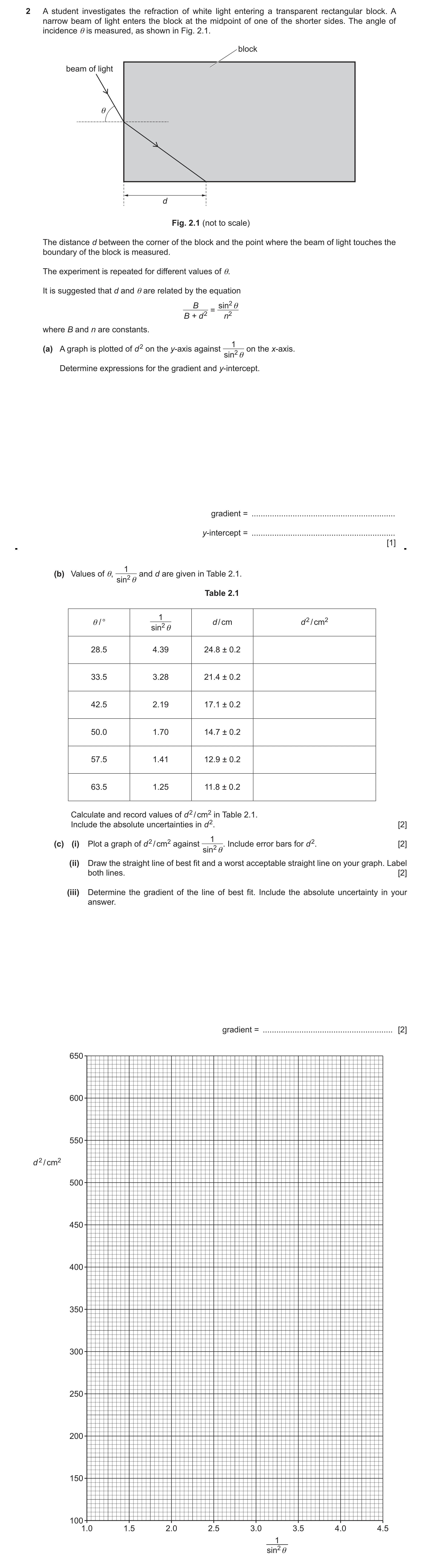
Q14 · A student investigates the refraction of white light entering a transparent rectangular… 9702/52 Oct/Nov 2024
2 A student investigates the refraction of white light entering a transparent rectangular block. A narrow beam of light enters the block at the midpoint of one of the shorter sides. The angle of incidence θ is measured, as shown in Fig. 2.1. block beam of light θ d Fig. 2.1 (not to scale) The distance d between the corner of the block and the point where the beam of light touches the boundary of the block is measured. The experiment is repeated for different values of θ. It is suggested that d and θ are related by the equation B sin2 θ = B + d 2 n2 where B and n are constants. 1 (a) A graph is plotted of d 2 on the y-axis against on the x-axis. sin2 θ Determine expressions for the gradient and y-intercept. gradient = … y-intercept = … [1] 1 (b) Values of θ, and d are given in Table 2.1. sin2 θ Table 2.1 1 θ / ° d / cm d 2 / cm2 sin2 θ 28.5 4.39 24.8 ± 0.2 33.5 3.28 21.4 ± 0.2 42.5 2.19 17.1 ± 0.2 50.0 1.70 14.7 ± 0.2 57.5 1.41 12.9 ± 0.2 63.5 1.25 11.8 ± 0.2 Calculate and record values of d 2 / cm2 in Table 2.1. Include the absolute uncertainties in d 2. [2] 1(c) (i) Plot a graph of d 2 / cm2 against sin2 θ. Include error bars for d 2. [2] (ii) Draw the straight line of best fit and a worst acceptable straight line on your graph. Label both lines. [2] (iii) Determine the gradient of the line of best fit. Include the absolute uncertainty in your answer. gradient = … [2]
9 marks
Mark scheme: 2(a) gradient = Bn2 1 y-intercept = − B 2(b) 1 d2 / cm2 615 or 615.0 458 or 458.0 292 or 292.4 216 or 216.1 166 or 166.4 139 or 139.2 Values correct as shown above. Uncertainties in d2 decreasing from 10 to 4 or 5. 1 2(c)(i) Six points from (b) plotted correctly. 1 Must be within half a small square. Diameter of points must be less than half a small square. Error bars in d2 plotted correctly. 1 All error bars to be plotted. Total length of bar must be accurate to less than half a small square and symmetrical. 2(c)(ii) Straight line of best fit drawn. 1 Do not accept line from top point to bottom point. Points must be balanced. Line must pass between (1.90, 250) and (2.00, 250) and between (3.55, 500) and (3.65, 500). Worst acceptable line drawn (steepest or shallowest possible line that passes through all the error bars). 1 All error bars must be plotted. 2(c)(iii) Gradient determined with clear substitution of data points into y / x. 1 Distance between data points must be greater than half the length of the drawn line. Gradient determined of worst acceptable line with clear substitution of data points into y / x. 1 uncertainty = (gradient of line of best fit – gradient of worst acceptable line) or uncertainty = ½ (steepest worst line gradient – shallowest worst line gradient) 2(c)(iv) y-intercept determined by substitution of correct point with consistent power of ten in m and x into y = mx + c. 1 y-intercept of worst acceptable line determined by substitution into y = mx + c. 1 uncertainty = y-intercept of line of best fit – y-intercept of worst acceptable line or uncertainty = ½ (steepest worst line y-intercept – shallowest worst line y-intercept) Do not accept ECF from false origin method. 2(d)(i) B determined using y-intercept (B = – y-intercept) and B and n given to 2 or 3 or 4 significant figures. 1 n determined using gradient 1 and B and n given with SI units with correct powers of ten. gradient gradient n = or n = B − y -intercept Unit for B: cm2 No unit for n. 2(d)(ii) Percentage uncertainty in n determined with method shown. 1 1 y -intercept gradient percentage uncertainty = + 100 2 y -intercept gradient or correct substitution for max/min methods. 2(e) determined to a minimum of two significant figures from (c)(iii) and (c)(iv) or (d)(i) with correct substitution and correct 1 power of ten. −1 gradient = sin − y -intercept + 900 or −1 n 2 B = sin B + 900
This question in 9702/52 Oct/Nov 2024
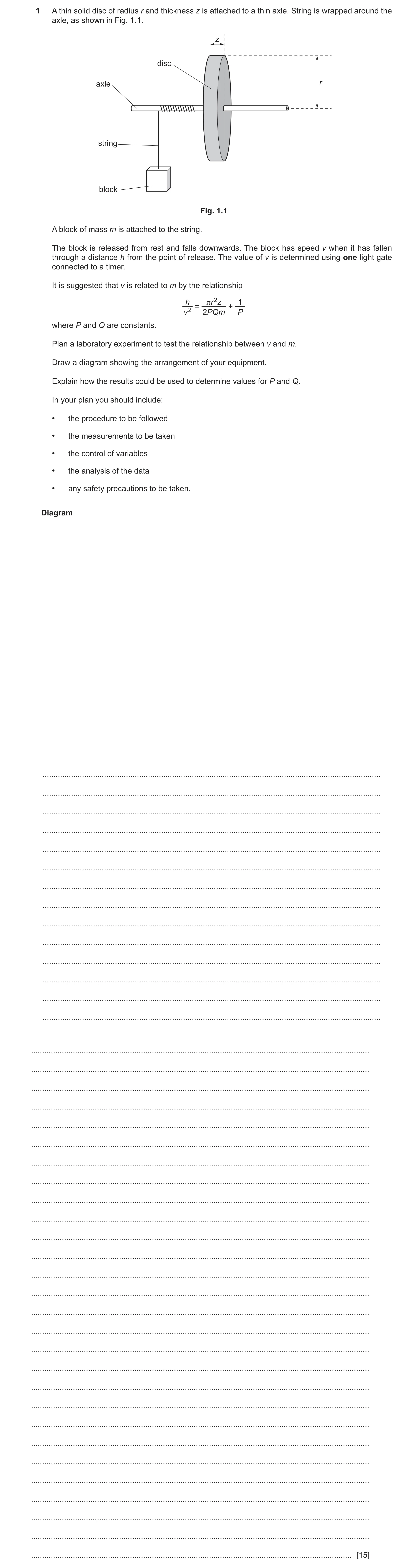
Q15 · A thin solid disc of radius r and thickness z is attached to a thin axle 9702/52 May/June 2025
1 A thin solid disc of radius r and thickness z is attached to a thin axle. String is wrapped around the axle, as shown in Fig. 1.1. z disc axle r string block Fig. 1.1 A block of mass m is attached to the string. The block is released from rest and falls downwards. The block has speed v when it has fallen through a distance h from the point of release. The value of v is determined using one light gate connected to a timer. It is suggested that v is related to m by the relationship h πr 2z 1 = + v 2 2PQm P where P and Q are constants. Plan a laboratory experiment to test the relationship between v and m. Draw a diagram showing the arrangement of your equipment. Explain how the results could be used to determine values for P and Q. In your plan you should include: • the procedure to be followed • the measurements to be taken • the control of variables • the analysis of the data • any safety precautions to be taken. Diagram … … … … … … … … … … … … … … … … … … … … … … … … … … … … … … … … … … … … … … … … … … [15]
15 marks
Mark scheme: Question Answer Marks 1 Defining the problem vary m and measure v or m is the independent variable and v is the dependent variable 1 keep h constant 1 Methods of data collection labelled diagram of workable experiment including: 1 • axle resting on support(s) (on stands) • supports placed on bench • light gate (connected to timer) positioned at a distance h • light gate labelled and h indicated vertical metre rule clamped to a stand in a position close to block to measure h 1 method to determine v using an interrupt length, e.g. v = length of block / time recorded by the timer 1 method to measure m, e.g. use a (top-pan) balance 1 Method of analysis 1 1 1 plot a graph of against or equivalent v 2 m Do not accept logarithms. 1 1 1 1 1 1 against against v 2 m m v 2 1 gradient P = P = − h y -intercept y -intercept h or r 2 z gradient P = 2Qh 1 1 1 1 1 against against v 2 m m v 2 r 2 z r 2 z y -intercept Q = Q = − 2Ph gradient 2 or r 2 z y -intercept Q = 2 gradient Additional detail including safety considerations 6 D1 precaution linked to falling block resulting in damage to block / bench, e.g. use a cushion / sand tray to prevent damage to bench or precaution linked to stands falling, e.g. clamp stand(s) to the bench prevent stand falling D2 keep r and z constant D3 method to determine r e.g. use calipers / ruler to measure diameter d and r = d / 2 D4 measure z with a micrometer / calipers 1 D5 set square correctly positioned between rule and bench to ensure that rule to measure h is vertical D6 method to keep h constant by identifying constant initial position of the bottom of the block, e.g. clamped pin / rod to indicate the starting point each time or (fiducial) marker on rule D7 description of method to ensure that axle can rotate, e.g. axle is lubricated at the supports to enable axle to rotate, axle is not fixed at the supports so axle can rotate D8 use a large length of block to reduce (percentage) uncertainty in interrupt time or increase the time light gate is interrupted D9 repeat experiment for the same value of m and determine the average v 1 D10 relationship valid if a straight line is produced (with y-intercept = ). hP Do not accept line passing through the origin.
This question in 9702/52 May/June 2025
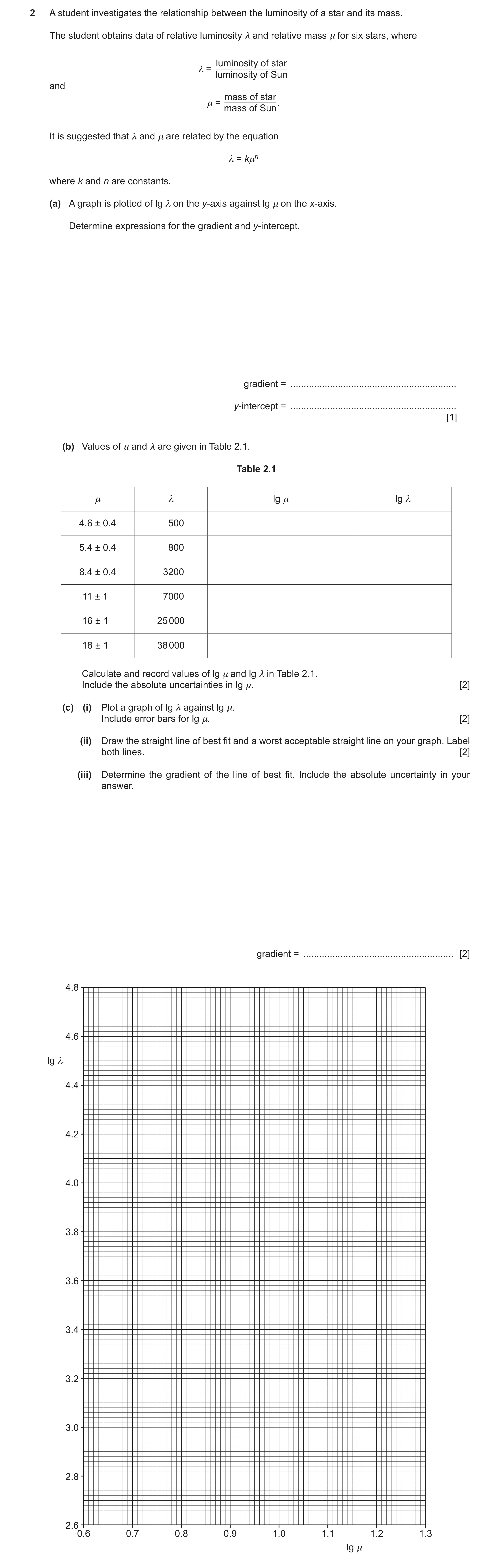
Q16 · A student investigates the relationship between the luminosity of a star and its mass 9702/54 May/June 2025
2 A student investigates the relationship between the luminosity of a star and its mass. The student obtains data of relative luminosity λ and relative mass µ for six stars, where luminosity of star λ = luminosity of Sun and mass of star µ = mass of Sun. It is suggested that λ and µ are related by the equation λ = kµn where k and n are constants. (a) A graph is plotted of lg λ on the y-axis against lg µ on the x-axis. Determine expressions for the gradient and y-intercept. gradient = … y-intercept = … [1] (b) Values of µ and λ are given in Table 2.1. Table 2.1 µ λ lg µ lg λ 4.6 ± 0.4 500 5.4 ± 0.4 800 8.4 ± 0.4 3200 11 ± 1 7000 16 ± 1 25 000 18 ± 1 38 000 Calculate and record values of lg µ and lg λ in Table 2.1. Include the absolute uncertainties in lg µ. [2] (c) (i) Plot a graph of lg λ against lg µ. Include error bars for lg µ. [2] (ii) Draw the straight line of best fit and a worst acceptable straight line on your graph. Label both lines. [2] (iii) Determine the gradient of the line of best fit. Include the absolute uncertainty in your answer. gradient = … [2]
9 marks
Mark scheme: 2(a) gradient = n 1 y-intercept = lg k 2(b) 1 lg lg 0.66 or 0.663 0.04 2.70 or 2.699 0.73 or 0.732 0.03 2.90 or 2.903 0.92 or 0.924 0.02 3.51 or 3.505 1.04 or 1.041 0.04 3.85 or 3.845 1.20 or 1.204 0.03 4.40 or 4.398 1.26 or 1.255 0.02 or 0.03 4.58 or 4.580 Values of lg and lg correct as shown above. Uncertainties in lg correct as shown above. 1 2(c)(i) Six points from (b) plotted correctly. 1 Must be within half a small square. Diameter of points must be less than half a small square. Error bars in lg plotted correctly. 1 All error bars must be plotted. Total length of bar must be accurate to less than half a small square and symmetrical. 2(c)(ii) Straight line of best fit drawn. 1 Thickness of the line must be less than half a small square. Do not accept line from top point to bottom point. Line must pass between (0.82, 3.20) and (0.84, 3.20) and between (1.13, 4.20) and (1.16, 4.20). Worst acceptable straight line drawn (steepest or shallowest possible line that passes through all the error bars). 1 Thickness of the line must be less than half a small square. All error bars must be plotted. 2(c)(iii) Gradient determined with clear substitution of data points into y / x. 1 Distance between data points must be greater than half the length of the drawn line. Gradient determined of worst acceptable line with clear substitution of data points into y / x. 1 uncertainty = (gradient of line of best fit – gradient of worst acceptable line) or uncertainty = ½ (steepest worst line gradient – shallowest worst line gradient) 2(c)(iv) y-intercept determined by substitution of correct point with consistent power of ten in m and x into y = mx + c. 1 y-intercept of worst acceptable line determined by substitution into y = mx + c. 1 uncertainty = y-intercept of line of best fit – y-intercept of worst acceptable line or uncertainty = ½ (steepest worst line y-intercept – shallowest worst line y-intercept) Do not allow methods using a false origin. 2(d) Value of k determined using y-intercept. 1 k = 10y −intercept n = gradient and n and k given to 2 or 3 significant figures. 1 absolute uncertainty in n = absolute uncertainty in gradient 1 and absolute uncertainty in k = (10y-intercept – 10y-intercept of WAL) Correct method must be seen. 2(e) M determined to a minimum of 2 significant figures from (d) or (c)(iii) and (c)(iv) with correct substitution and correct 1 power(s) of ten. Do not accept incorrect POT for n or k. Correct substitution must be seen. 0.46 lg0.46 − y -intercept lg0.46 − lg k = n = gradient or lg = or lg = k (d) gradient gradient and M = 2.0 1030
This question in 9702/54 May/June 2025
Q17 · On a bench, a steel ball of radius r is used to compress a spring by a distance x 9702/51 Oct/Nov 2025
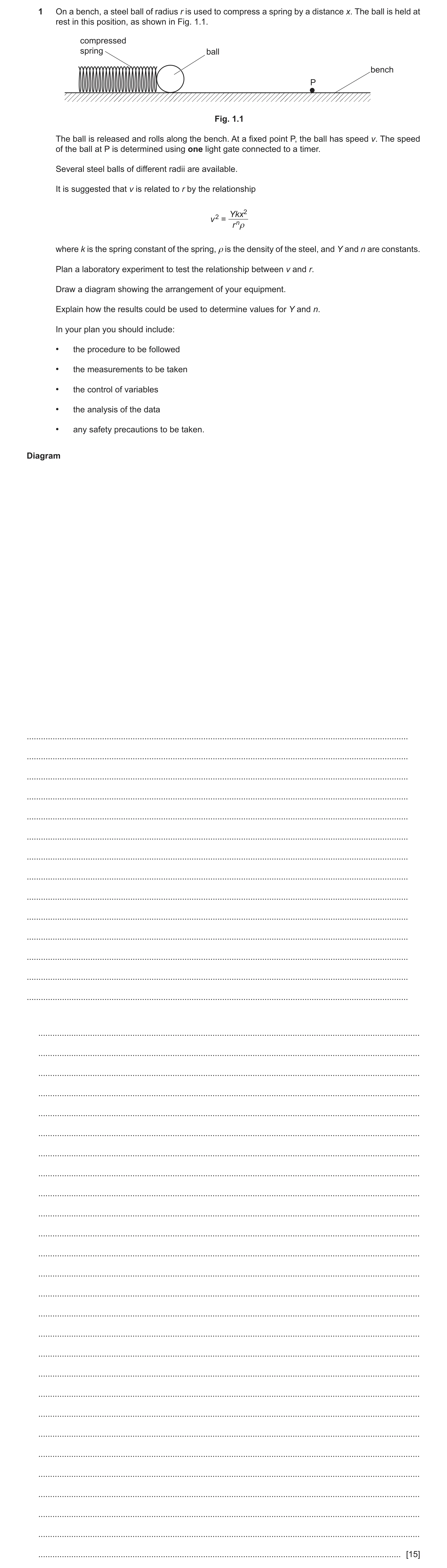
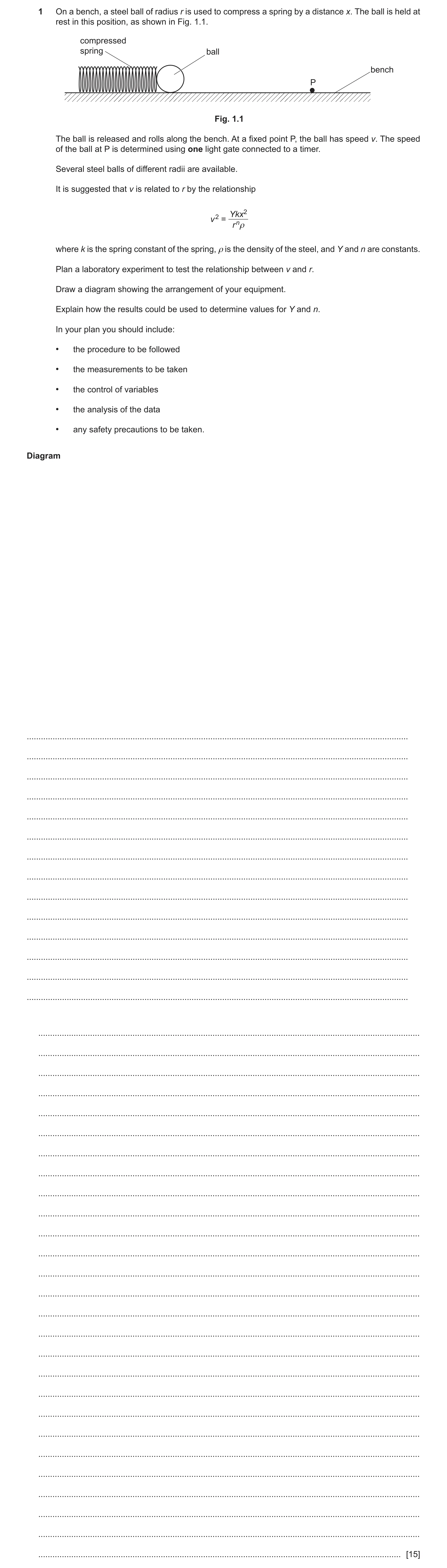
1 On a bench, a steel ball of radius r is used to compress a spring by a distance x. The ball is held at rest in this position, as shown in Fig. 1.1. compressed spring ball bench P Fig. 1.1 The ball is released and rolls along the bench. At a fixed point P, the ball has speed v. The speed of the ball at P is determined using one light gate connected to a timer. Several steel balls of different radii are available. It is suggested that v is related to r by the relationship Ykx2 v 2 = r nρ where k is the spring constant of the spring, ρ is the density of the steel, and Y and n are constants. Plan a laboratory experiment to test the relationship between v and r. Draw a diagram showing the arrangement of your equipment. Explain how the results could be used to determine values for Y and n. In your plan you should include: • the procedure to be followed • the measurements to be taken • the control of variables • the analysis of the data • any safety precautions to be taken. Diagram … … … … … … … … … … … … … … … … … … … … … … … … … … … … … … … … … … … … … … … … … [15]
15 marks
Mark scheme: Question Answer Marks 1 Defining the problem vary r and measure v or r is the independent variable and v is the dependent variable 1 keep x constant 1 Methods of data collection labelled diagram of workable experiment including: 1 • one end of spring resting against block clamped to bench using G-clamp • light gate positioned at P • light gate connected to timer • apparatus shown on bench • labels for light gate and P and at least one other label from bench, block, stand, spring, ball, timer method to determine r, e.g. use calipers or micrometer to measure diameter d and r = d / 2 1 description of method to determine v, use diameter of ball (to interrupt beam) ÷ measured time at light gate positioned at P 1 instrument to determine x, e.g. rule(r) or calipers 1 Method of Analysis plot a graph of (2 lg v) or (lg v2) against lg r 1 or plot a graph of (lg v) against (lg r) or equivalent, e.g. (ln v) against (ln r) n = −gradient for (2 lg v) or (lg v2) against lg r 1 or n = −2 gradient for (lg v) against lg r 1 10y -intercept 1 Y = for (2 lg v) or (lg v2) against lg r kx 2 or 10 2 y -intercept Y = for (lg v) against lg r kx 2 Additional detail including safety considerations 6 D1 precaution to prevent ball leaving bench, e.g. screens around apparatus / cushions on bench (to stop the ball) D2 keep k and constant D3 description of method to determine k, e.g. add mass to spring and k = mg / extension or use newton meter to measure force applied to spring and k = force / extension or take several readings of force and extension, plot a force–extension graph and k = gradient m D4 description of experimental method to determine , e.g. measure mass of ball using a balance and = 4 3 r 3 D5 repeat measurements of diameter or d in different directions and determine the average value of d D6 method to keep x constant, e.g. use a pin / ruler / card to indicate the starting point each time to keep x constant D7 x = original length of spring – compressed length of spring D8 adjust (vertical) position of light gate so that the diameter of (each) ball cuts the beam D9 repeat experiment for the same value of r and determine the average v 1 Ykx 2 1 Ykx 2 D10 relationship valid if a straight line is produced (with y-intercept = lg or lg ). 2 Do not accept line through the origin.
This question in 9702/51 Oct/Nov 2025
Q18 · A model wind turbine with blades, each of length L, placed in moving air 9702/52 Oct/Nov 2025
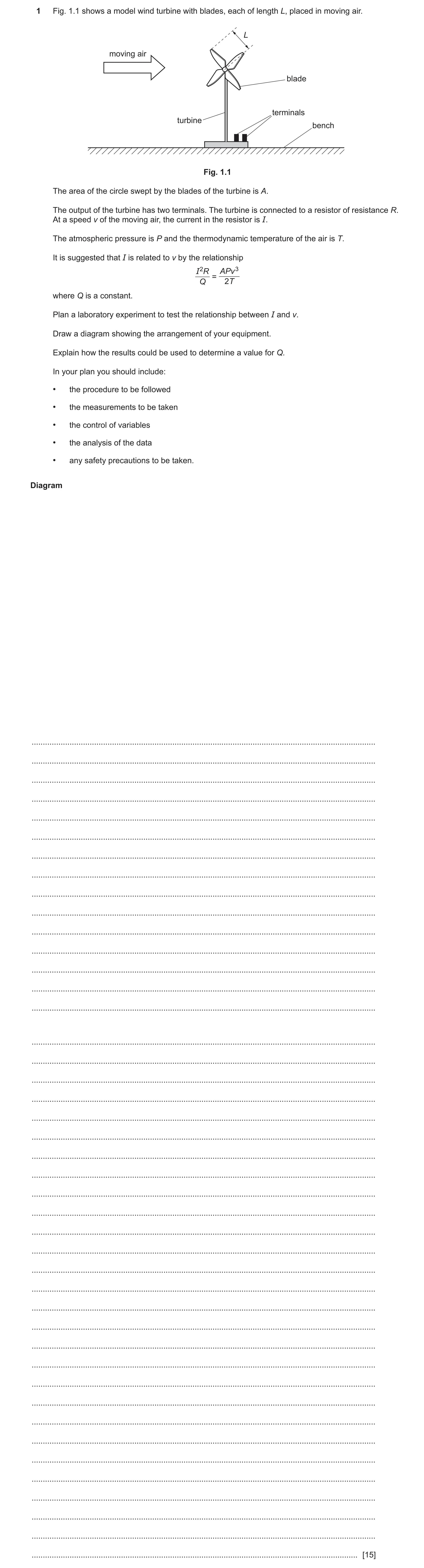
1 Fig. 1.1 shows a model wind turbine with blades, each of length L, placed in moving air. L moving air blade terminals turbine bench Fig. 1.1 The area of the circle swept by the blades of the turbine is A. The output of the turbine has two terminals. The turbine is connected to a resistor of resistance R. At a speed v of the moving air, the current in the resistor is I. The atmospheric pressure is P and the thermodynamic temperature of the air is T. It is suggested that I is related to v by the relationship I2R APv3 = Q 2T where Q is a constant. Plan a laboratory experiment to test the relationship between I and v. Draw a diagram showing the arrangement of your equipment. Explain how the results could be used to determine a value for Q. In your plan you should include: • the procedure to be followed • the measurements to be taken • the control of variables • the analysis of the data • any safety precautions to be taken. Diagram … … … … … … … … … … … … … … … … … … … … … … … … … … … … … … … … … … … … … … … … … … … [15]
15 marks
Mark scheme: Question Answer Marks 1 Defining the problem vary v and measure I or v is the independent variable and I is the dependent variable 1 keep A and R constant 1 Methods of data collection labelled diagram of workable experiment including: 1 • fan positioned in line with the turbine so that blades of both fan and turbine overlap • fan on bench • fan labelled and one other label from bench, turbine, blade(s) (of turbine), terminals, L workable circuit diagram showing resistor connected to an ammeter in series with the terminals of the turbine using correct 1 circuit symbols method to vary v, e.g. change speed of fan / change distance between fan and blades / vary current in or p.d. across fan 1 method to determine temperature T, e.g. use a thermometer 1 Method of Analysis plot a graph of I2 against v3 or equivalent (e.g. lg I against lg v or 2 ln I against ln v) 1 relationship valid if a straight line is produced passing through the origin 1 (For lg I against lg v: relationship valid if a straight line with gradient = 1.5 is produced) 2TR gradient 1 Q = AP 2TR 10 2 y -intercept (For lg I against lg v: Q = ) AP 1 Additional detail including safety considerations 6 D1 precaution with reason linked to (moving) fan blades / turbine blades, e.g. keep away from the fan to avoid (moving) blades or use a screen around the fan / turbine to avoid (moving) blades or precaution with reason linked to prevent air / dust particles in eye, e.g. use goggles to avoid air stream (into eye) D2 clamp turbine / fan to bench D3 keep P and T constant D4 T = t + 273 D5 method to determine A: use a rule(r) / calipers to measure L and A = L2 D6 repeat measurements of L in different positions / different blades and average D7 method to measure v, e.g. use an anemometer or air speed meter or method to measure P, e.g. use a manometer or barometer or pressure gauge D8 wait for steady / constant air flow / movement of blades / current D9 method to determine R, e.g.: separate circuit showing ohmmeter connected to R only or terminals of turbine connected correctly to resistor and ammeter and voltmeter across resistor and R = V / I or separate workable circuit with power supply resistor, ammeter and voltmeter across R and R = V / I D10 method to check temperature / pressure is constant, e.g. measure temperature / pressure several times / before and after
This question in 9702/52 Oct/Nov 2025
Q19 · On a bench, a steel ball of radius r is used to compress a spring by a distance x 9702/53 Oct/Nov 2025
1 On a bench, a steel ball of radius r is used to compress a spring by a distance x. The ball is held at rest in this position, as shown in Fig. 1.1. compressed spring ball bench P Fig. 1.1 The ball is released and rolls along the bench. At a fixed point P, the ball has speed v. The speed of the ball at P is determined using one light gate connected to a timer. Several steel balls of different radii are available. It is suggested that v is related to r by the relationship Ykx2 v 2 = r nρ where k is the spring constant of the spring, ρ is the density of the steel, and Y and n are constants. Plan a laboratory experiment to test the relationship between v and r. Draw a diagram showing the arrangement of your equipment. Explain how the results could be used to determine values for Y and n. In your plan you should include: • the procedure to be followed • the measurements to be taken • the control of variables • the analysis of the data • any safety precautions to be taken. Diagram … … … … … … … … … … … … … … … … … … … … … … … … … … … … … … … … … … … … … … … … … [15]
15 marks
Mark scheme: Question Answer Marks 1 Defining the problem vary r and measure v or r is the independent variable and v is the dependent variable 1 keep x constant 1 Methods of data collection labelled diagram of workable experiment including: 1 • one end of spring resting against block clamped to bench using G-clamp • light gate positioned at P • light gate connected to timer • apparatus shown on bench • labels for light gate and P and at least one other label from bench, block, stand, spring, ball, timer method to determine r, e.g. use calipers or micrometer to measure diameter d and r = d / 2 1 description of method to determine v, use diameter of ball (to interrupt beam) ÷ measured time at light gate positioned at P 1 instrument to determine x, e.g. rule(r) or calipers 1 Method of Analysis plot a graph of (2 lg v) or (lg v2) against lg r 1 or plot a graph of (lg v) against (lg r) or equivalent, e.g. (ln v) against (ln r) n = −gradient for (2 lg v) or (lg v2) against lg r 1 or n = −2 gradient for (lg v) against lg r 1 10y -intercept 1 Y = for (2 lg v) or (lg v2) against lg r kx 2 or 10 2 y -intercept Y = for (lg v) against lg r kx 2 Additional detail including safety considerations 6 D1 precaution to prevent ball leaving bench, e.g. screens around apparatus / cushions on bench (to stop the ball) D2 keep k and constant D3 description of method to determine k, e.g. add mass to spring and k = mg / extension or use newton meter to measure force applied to spring and k = force / extension or take several readings of force and extension, plot a force–extension graph and k = gradient m D4 description of experimental method to determine , e.g. measure mass of ball using a balance and = 4 3 r 3 D5 repeat measurements of diameter or d in different directions and determine the average value of d D6 method to keep x constant, e.g. use a pin / ruler / card to indicate the starting point each time to keep x constant D7 x = original length of spring – compressed length of spring D8 adjust (vertical) position of light gate so that the diameter of (each) ball cuts the beam D9 repeat experiment for the same value of r and determine the average v 1 Ykx 2 1 Ykx 2 D10 relationship valid if a straight line is produced (with y-intercept = lg or lg ). 2 Do not accept line through the origin.
This question in 9702/53 Oct/Nov 2025
Question 20 9702/54 Oct/Nov 2025
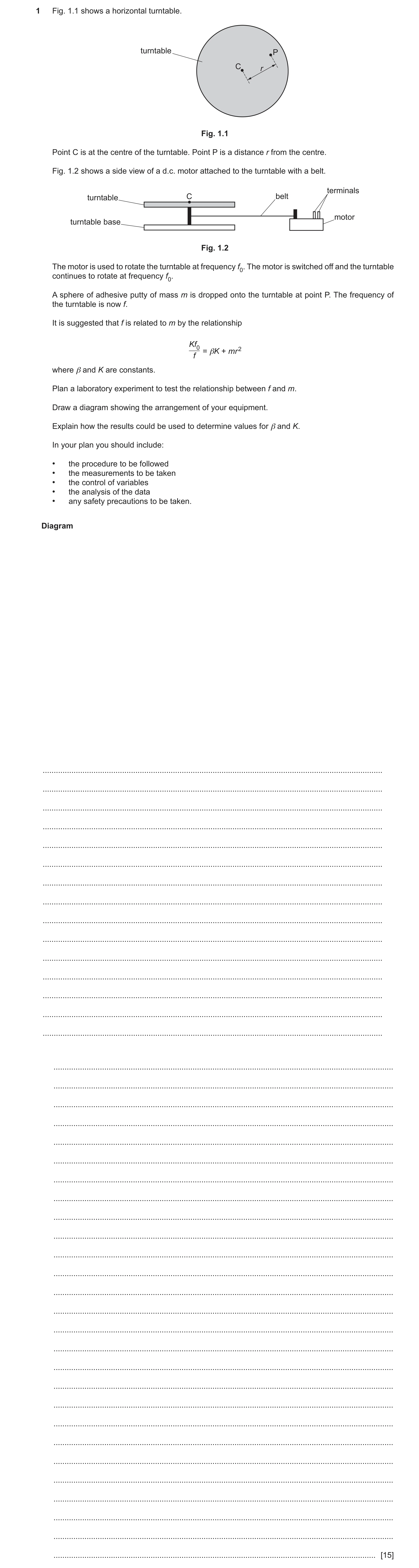
1 Fig. 1.1 shows a horizontal turntable. turntable P C r Fig. 1.1 Point C is at the centre of the turntable. Point P is a distance r from the centre. Fig. 1.2 shows a side view of a d.c. motor attached to the turntable with a belt. terminals turntable C belt motor turntable base Fig. 1.2 The motor is used to rotate the turntable at frequency f0. The motor is switched off and the turntable continues to rotate at frequency f0. A sphere of adhesive putty of mass m is dropped onto the turntable at point P. The frequency of the turntable is now f. It is suggested that f is related to m by the relationship Kf0 = βK + mr 2 f where β and K are constants. Plan a laboratory experiment to test the relationship between f and m. Draw a diagram showing the arrangement of your equipment. Explain how the results could be used to determine values for β and K. In your plan you should include: • the procedure to be followed • the measurements to be taken • the control of variables • the analysis of the data • any safety precautions to be taken. Diagram … … … … … … … … … … … … … … … … … … … … … … … … … … … … … … … … … … … … … … … … … … [15]
15 marks
Mark scheme: Question Answer Marks 1 Defining the problem vary m and measure f or m is the independent variable and f is the dependent variable 1 keep f0 constant 1 Methods of data collection labelled diagram of workable experiment including: 1 • turntable base and motor on bench • two labels from turntable, motor, belt, C, putty, bench, release mechanism workable circuit showing terminals of motor connected to (d.c.) supply 1 method to measure time to determine f and f0, e.g. use a stopwatch to measure (n)t 1 and method to measure m, e.g. use a (top-pan) balance measure the time t for n revolutions 1 and T = t / n and f = 1 / T or f = n / t Method of Analysis 1 1 plots a graph of against m or equivalent f Do not accept logarithms. 1 1 1 1 against m m against f f r 2 r 2 × gradient K = K = f0 × gradient f0 1 1 1 against m m against f f = f0 y -intercept f0 y -intercept = − gradient or r 2×y -intercept = − K 1 Additional detail including safety considerations 6 D1 precaution linked to putty leaving turntable, e.g. screens around apparatus / cushions to prevent putty from leaving bench D2 keep r constant D3 use rule(r) to measure r D4 stand and fixed point located above P (to ensure r is constant) D5 method to ensure putty is dropped at (constant) distance r, e.g.; fixed location above the turntable to drop putty to keep r constant or draw a circle of radius r on the turntable D6 method to keep f0 constant, e.g. adjust the rheostat to keep the current in the motor constant / check ammeter D7 clamp motor and/or turntable (base) to bench D8 lubricate the turntable to reduce friction D9 repeat experiment for the same value of m and determine the average f D10 relationship valid if a straight line is produced (with y-intercept = ) f0 Do not accept line through the origin.
This question in 9702/54 Oct/Nov 2025
 9
9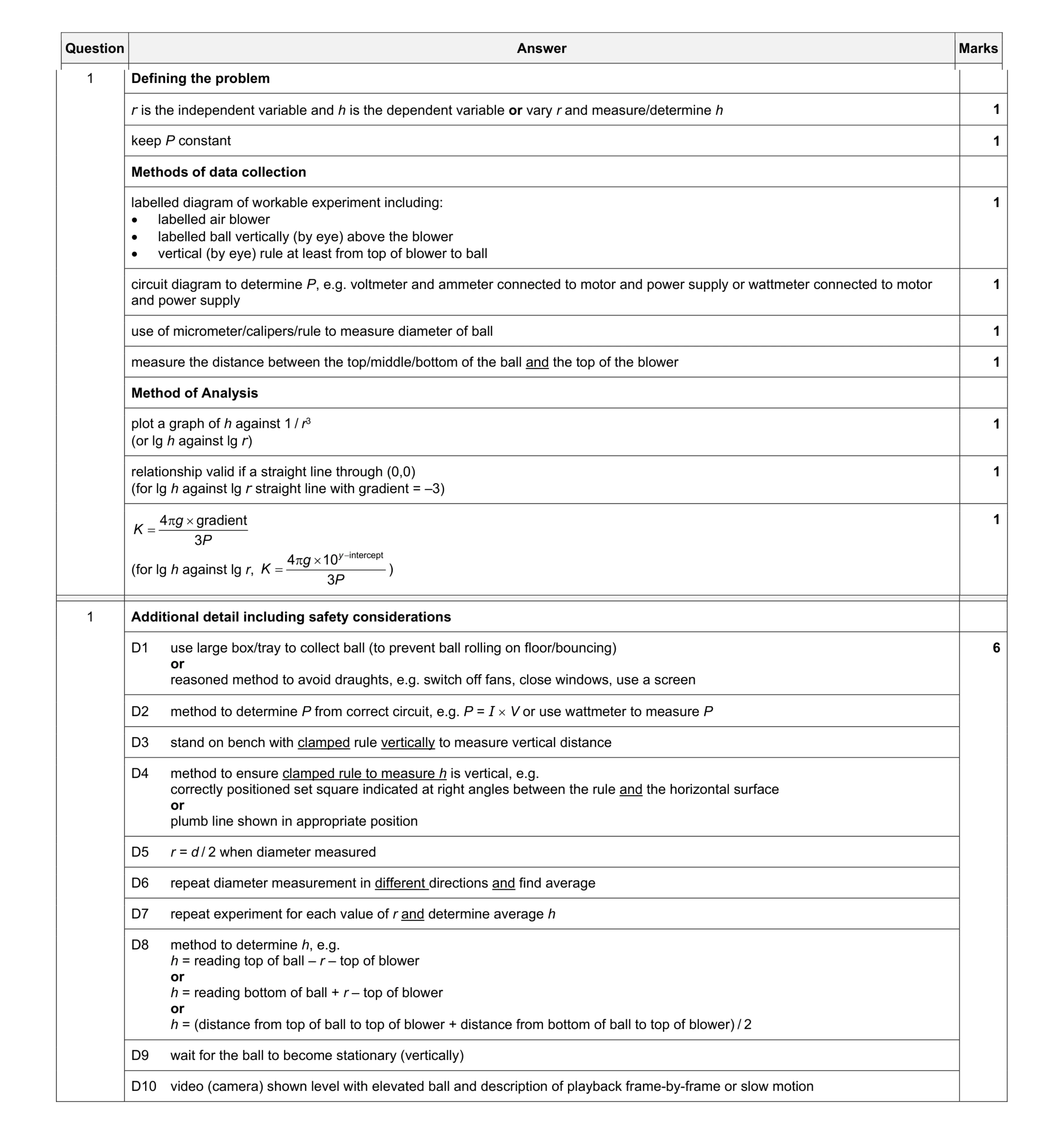 15
15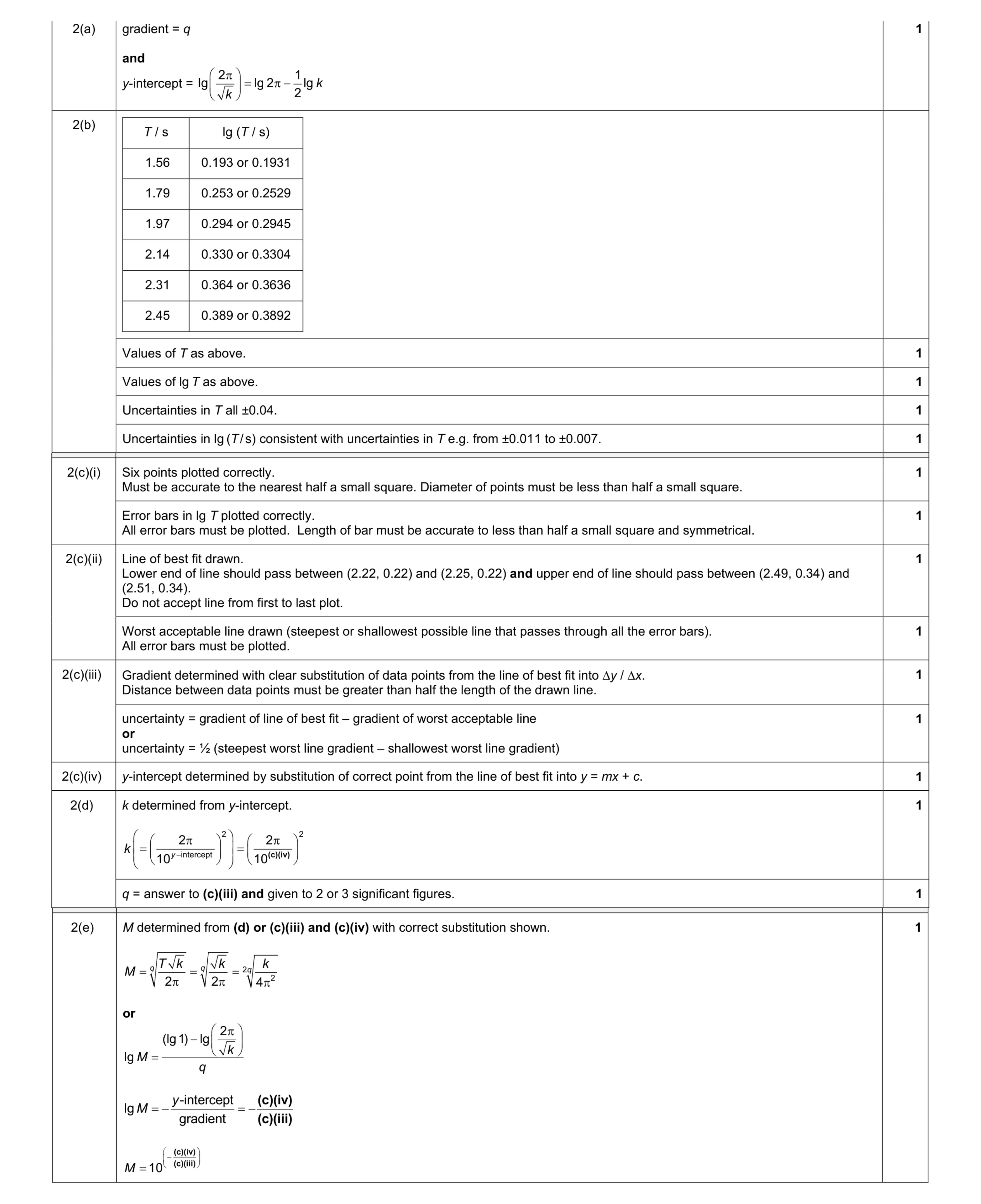 11
11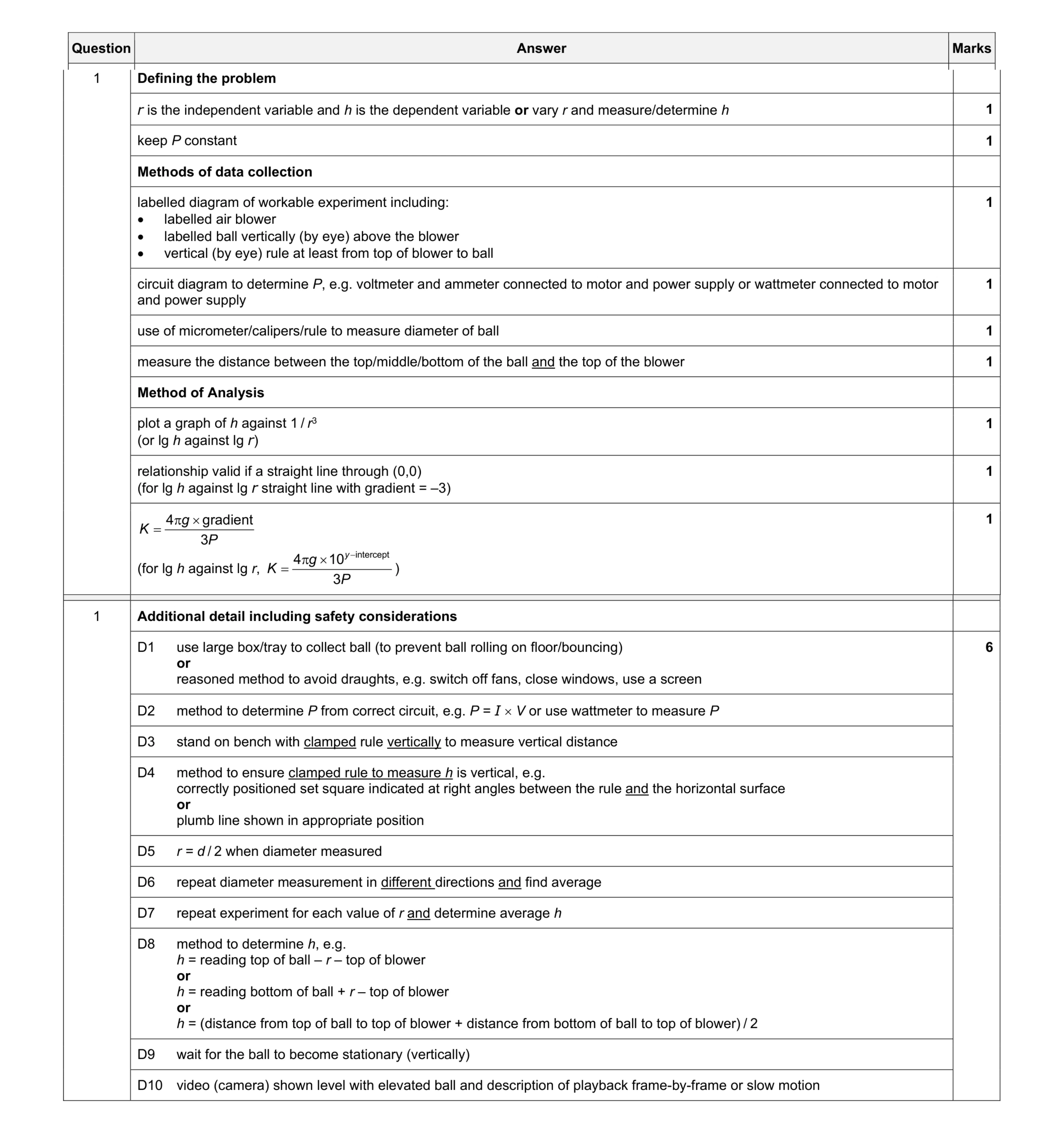 15
15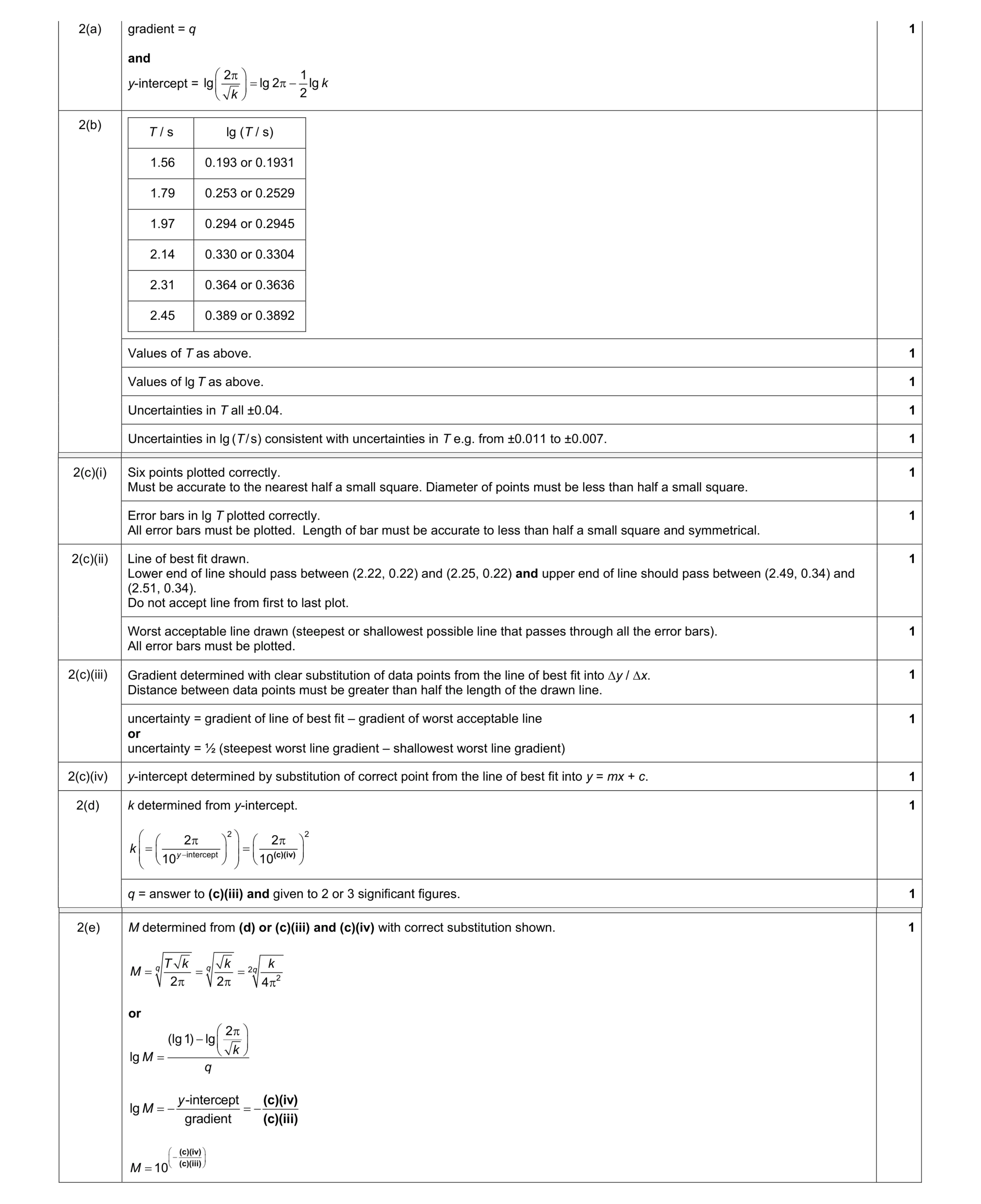 11
11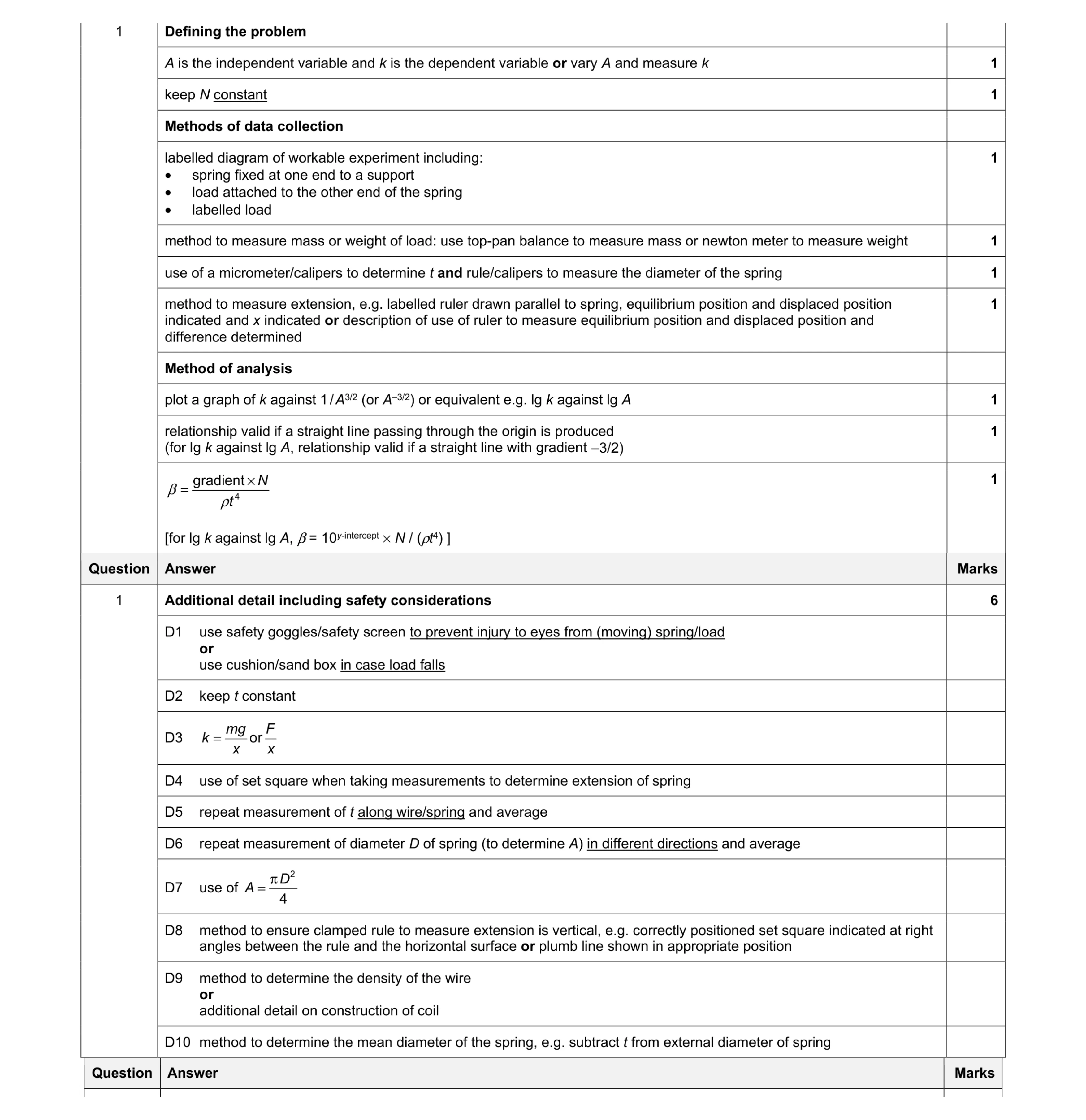 15
15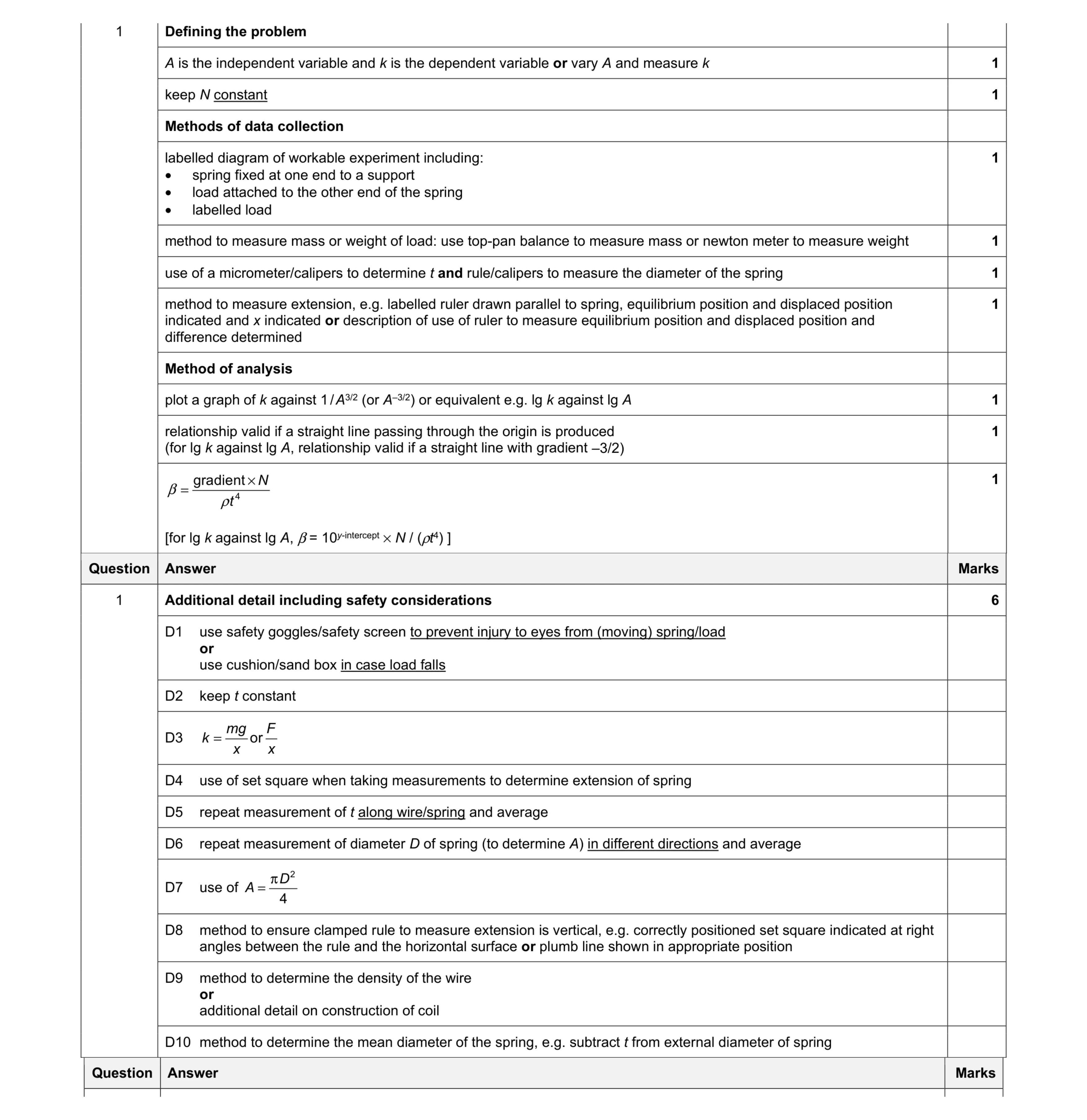 15
15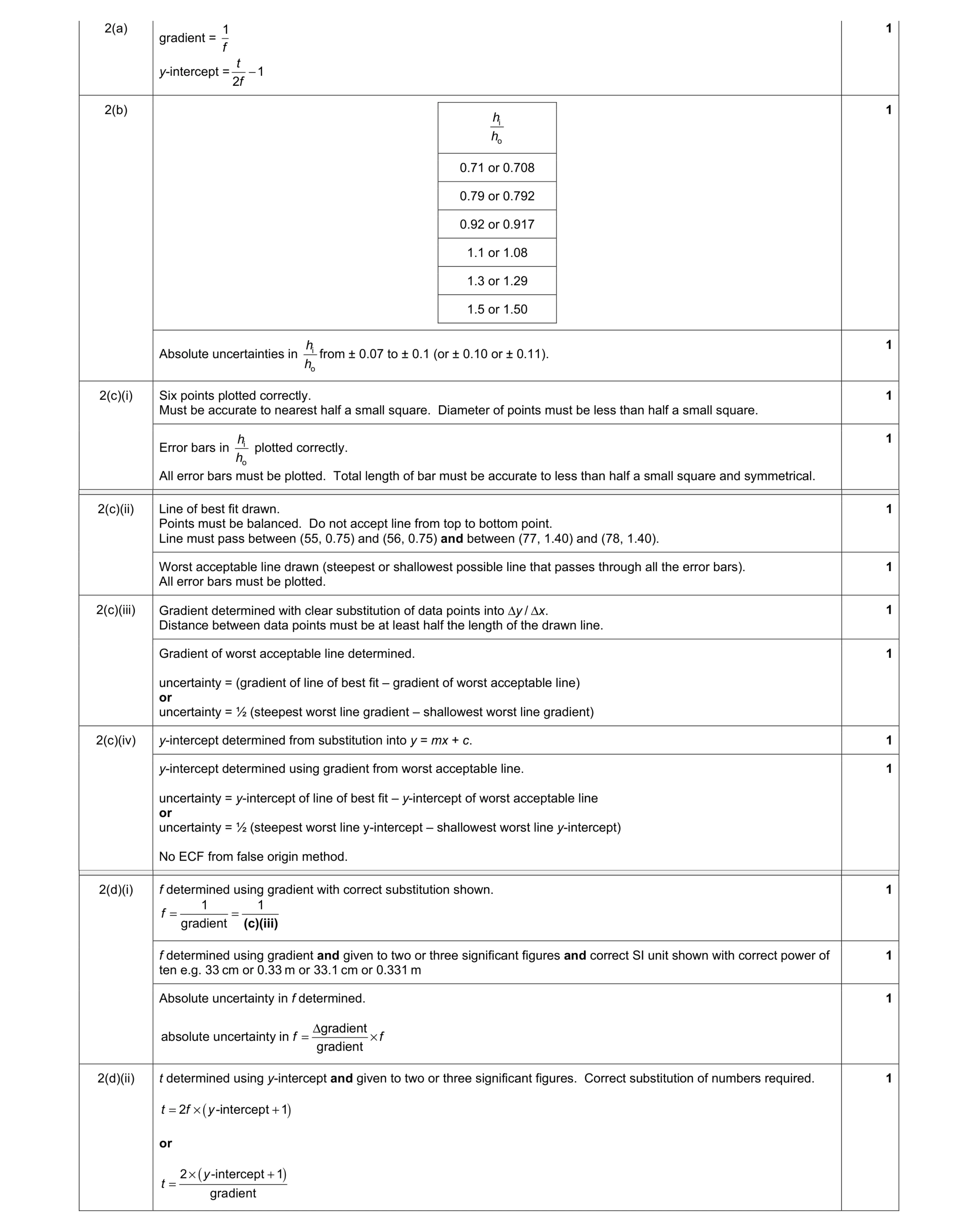 9
9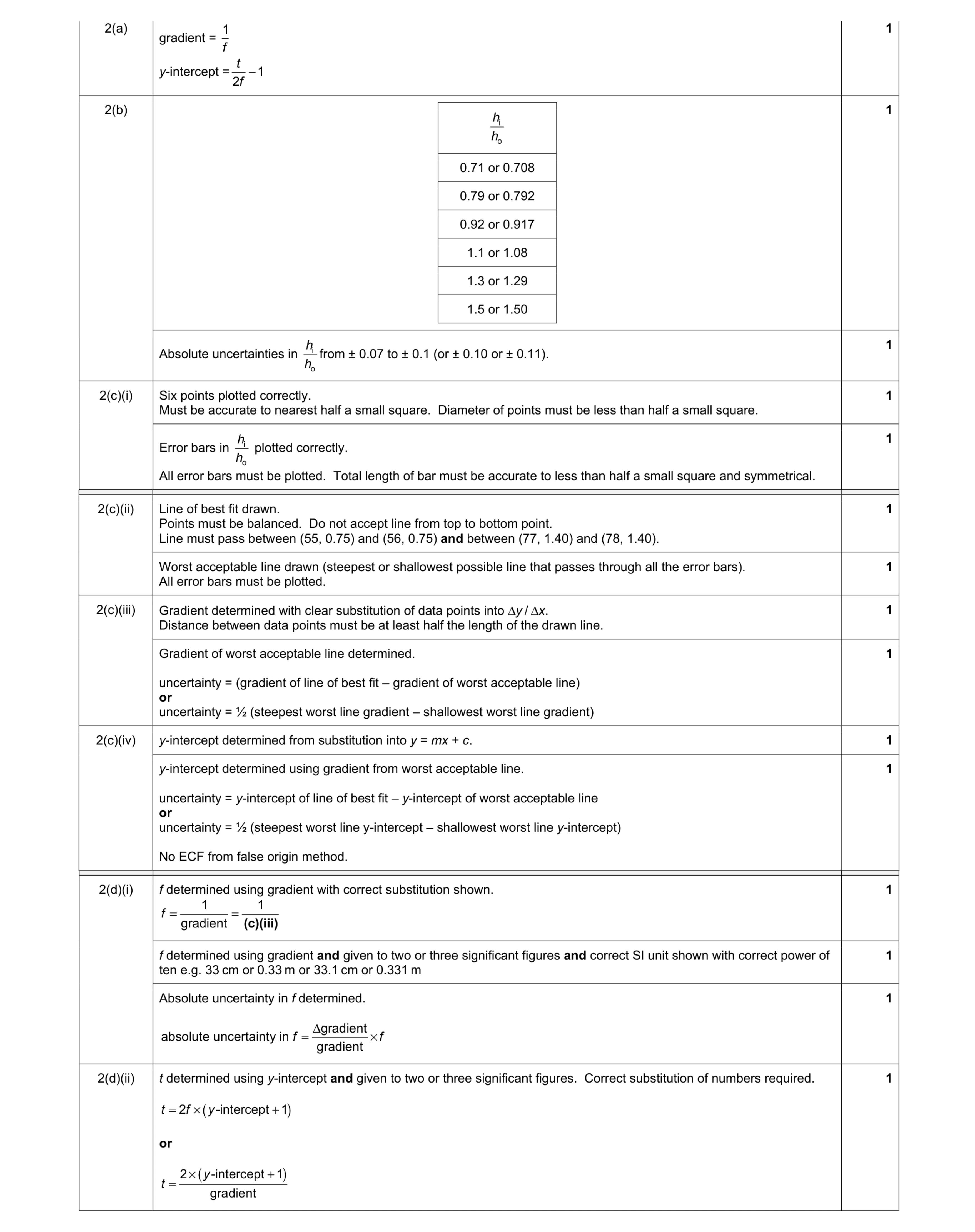 9
9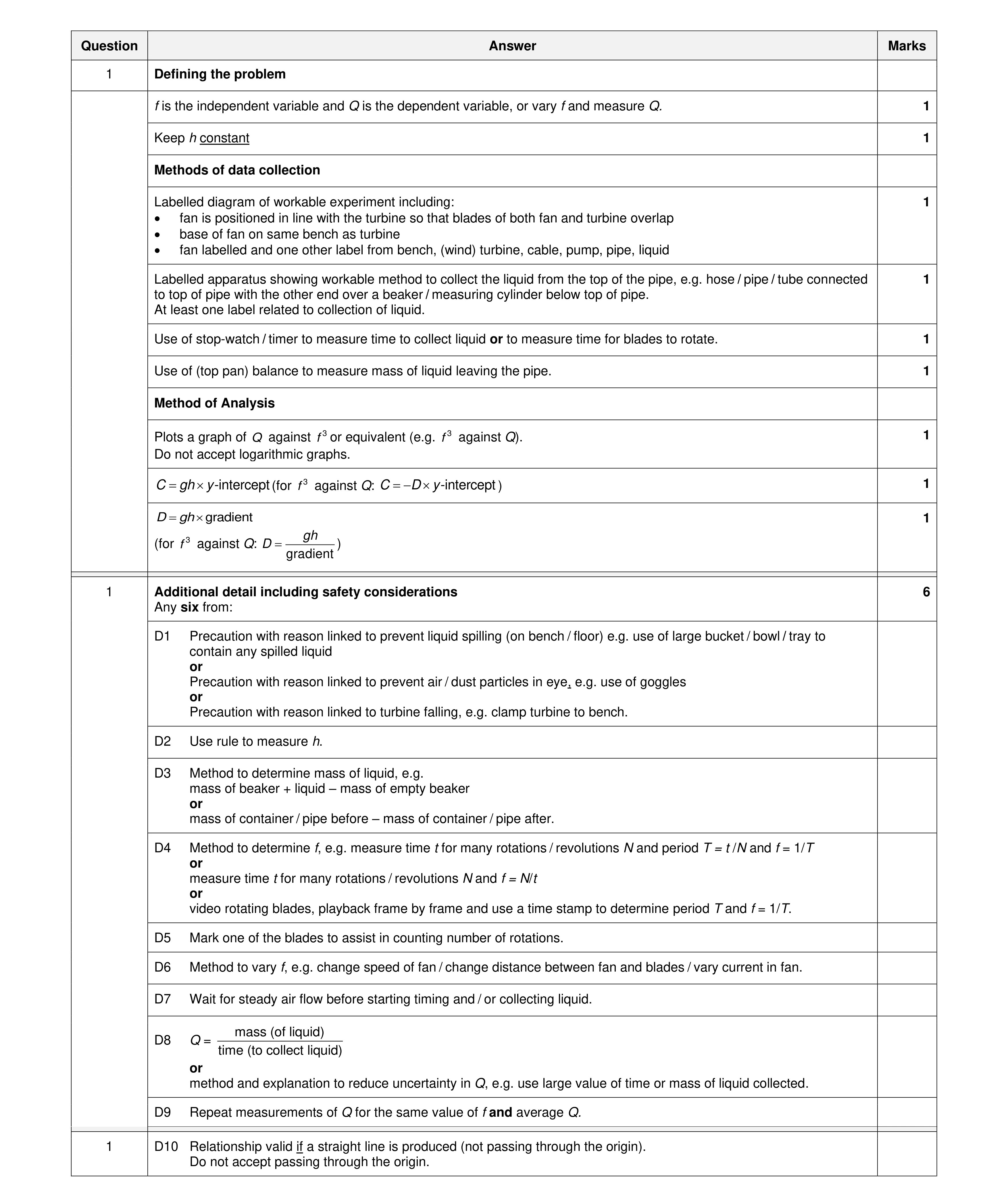 15
15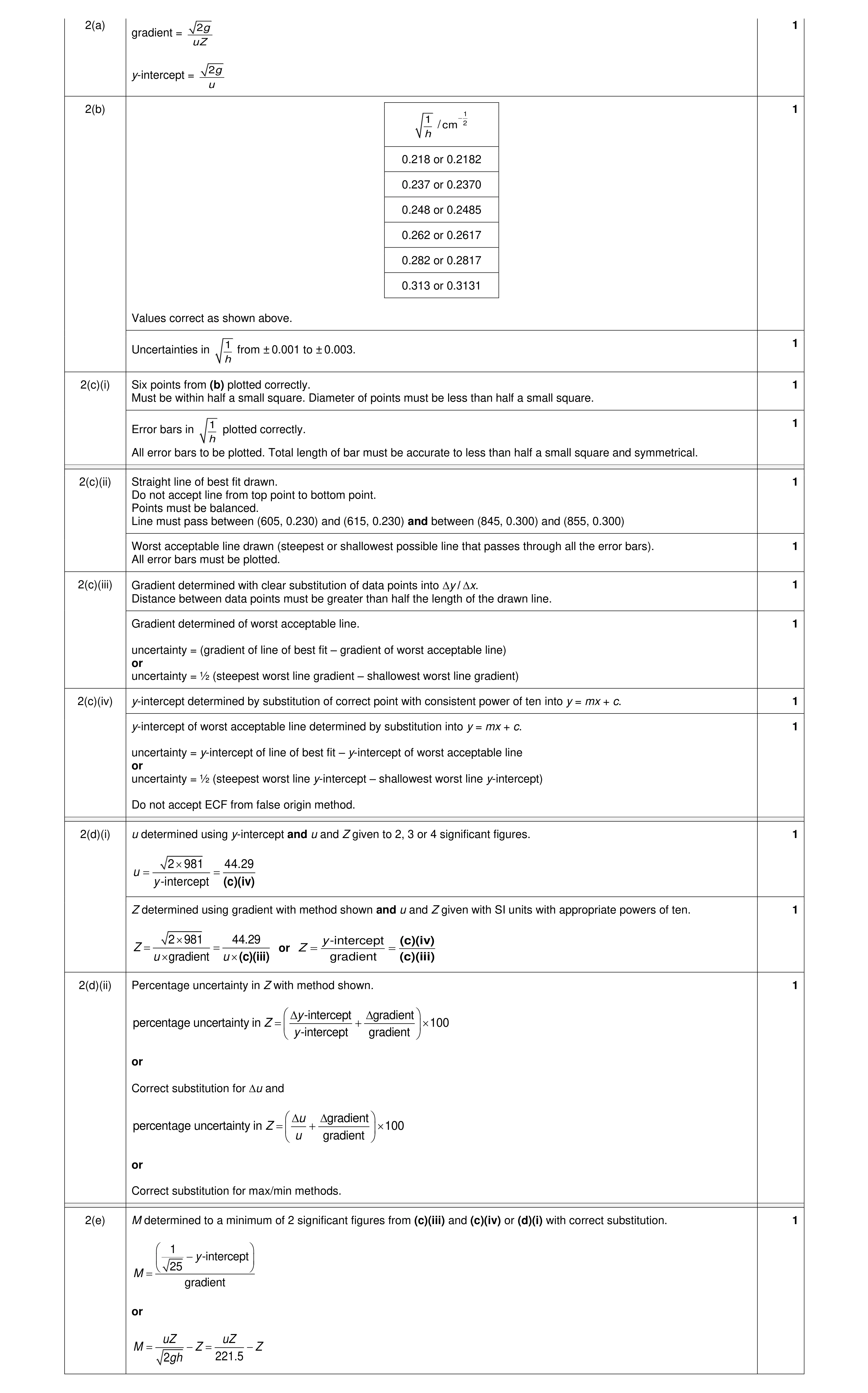 9
9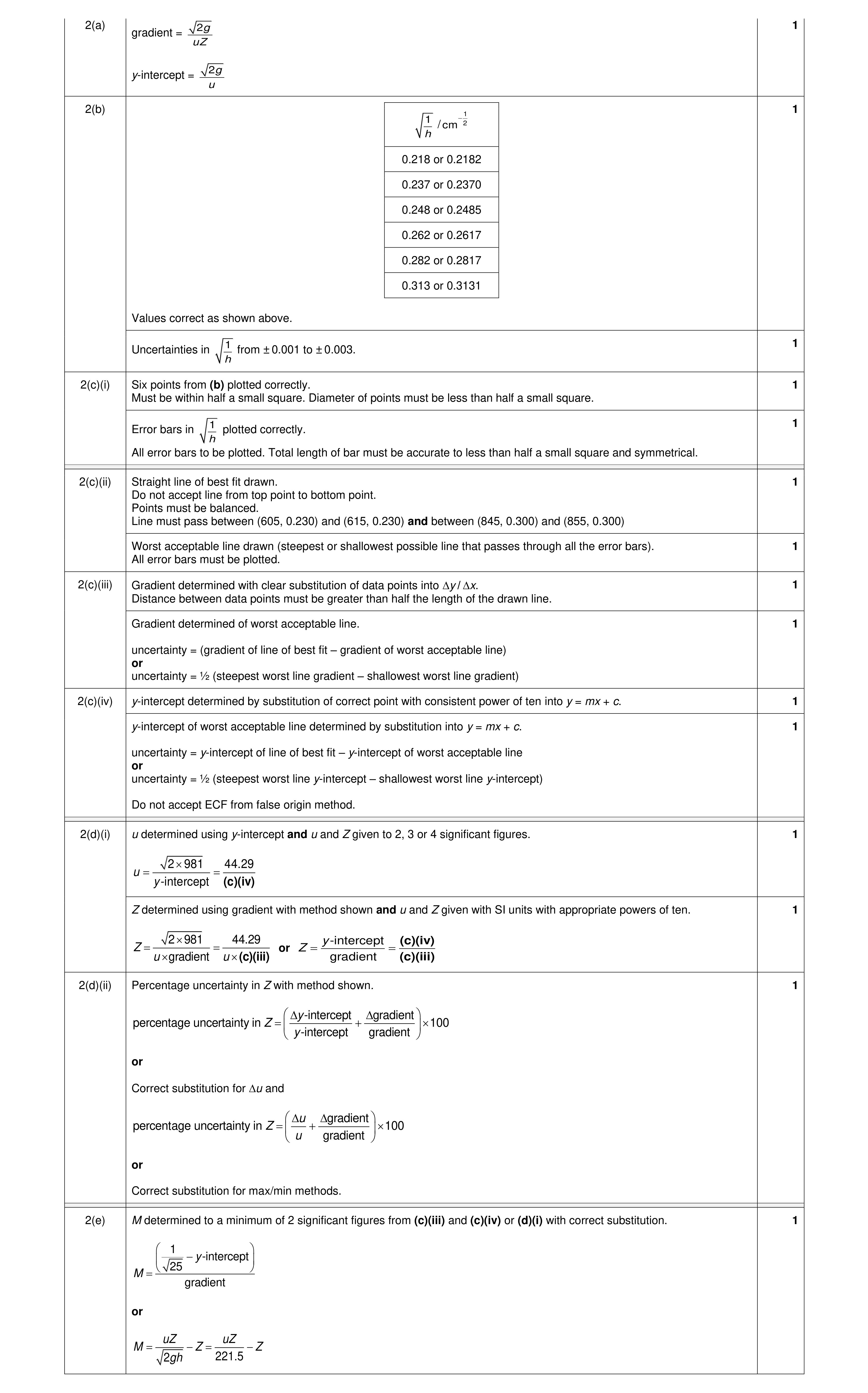 9
9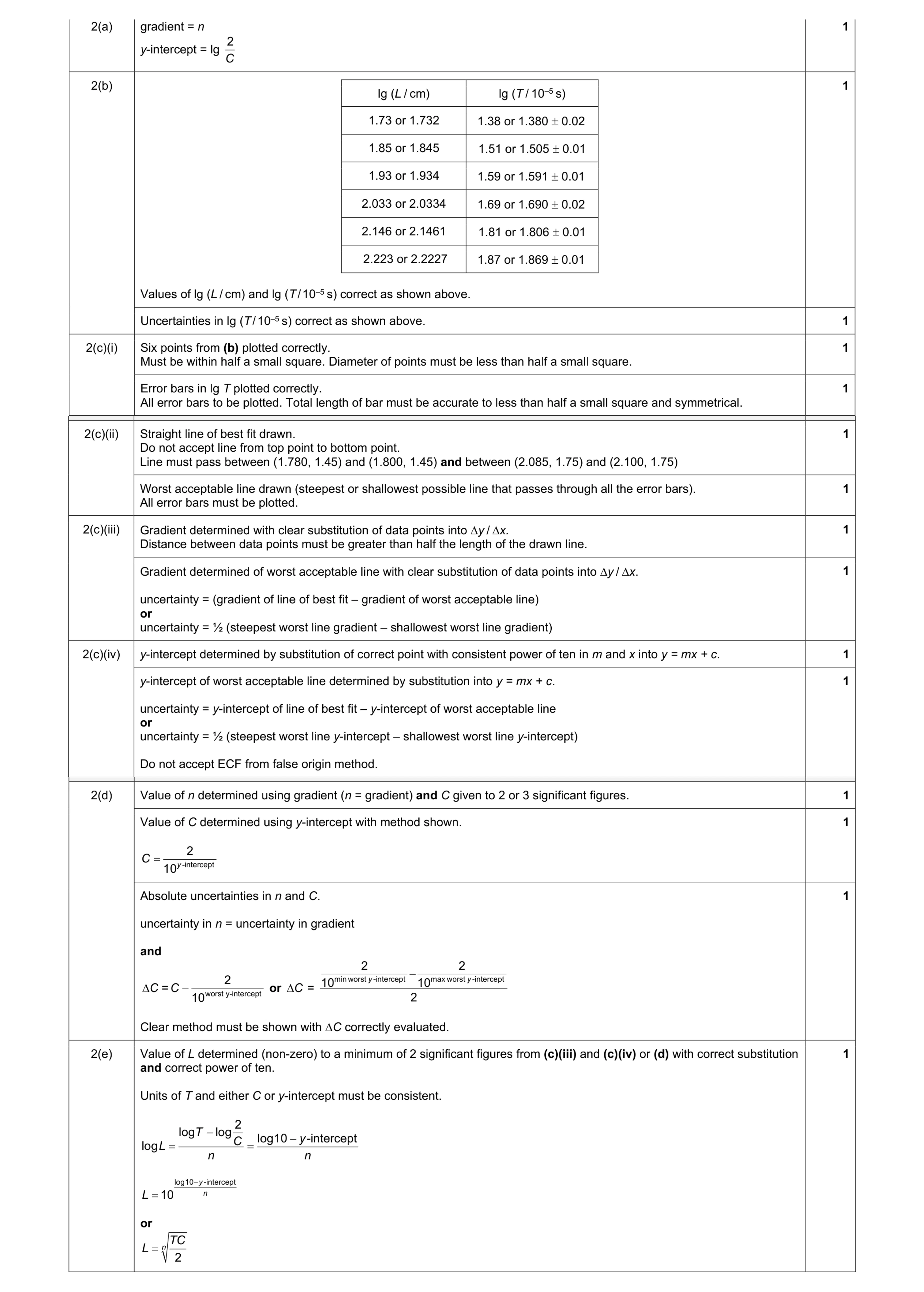 9
9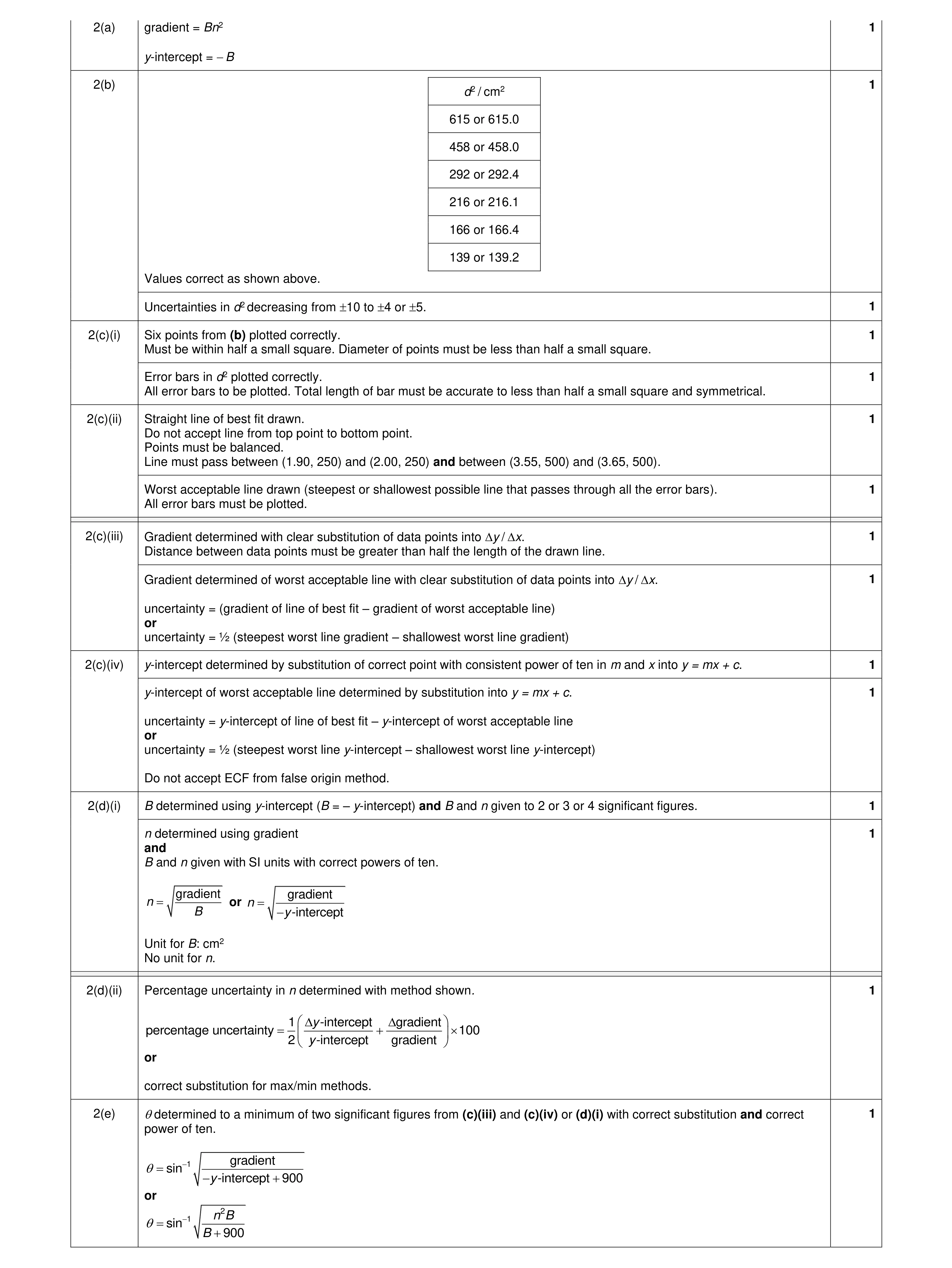 9
9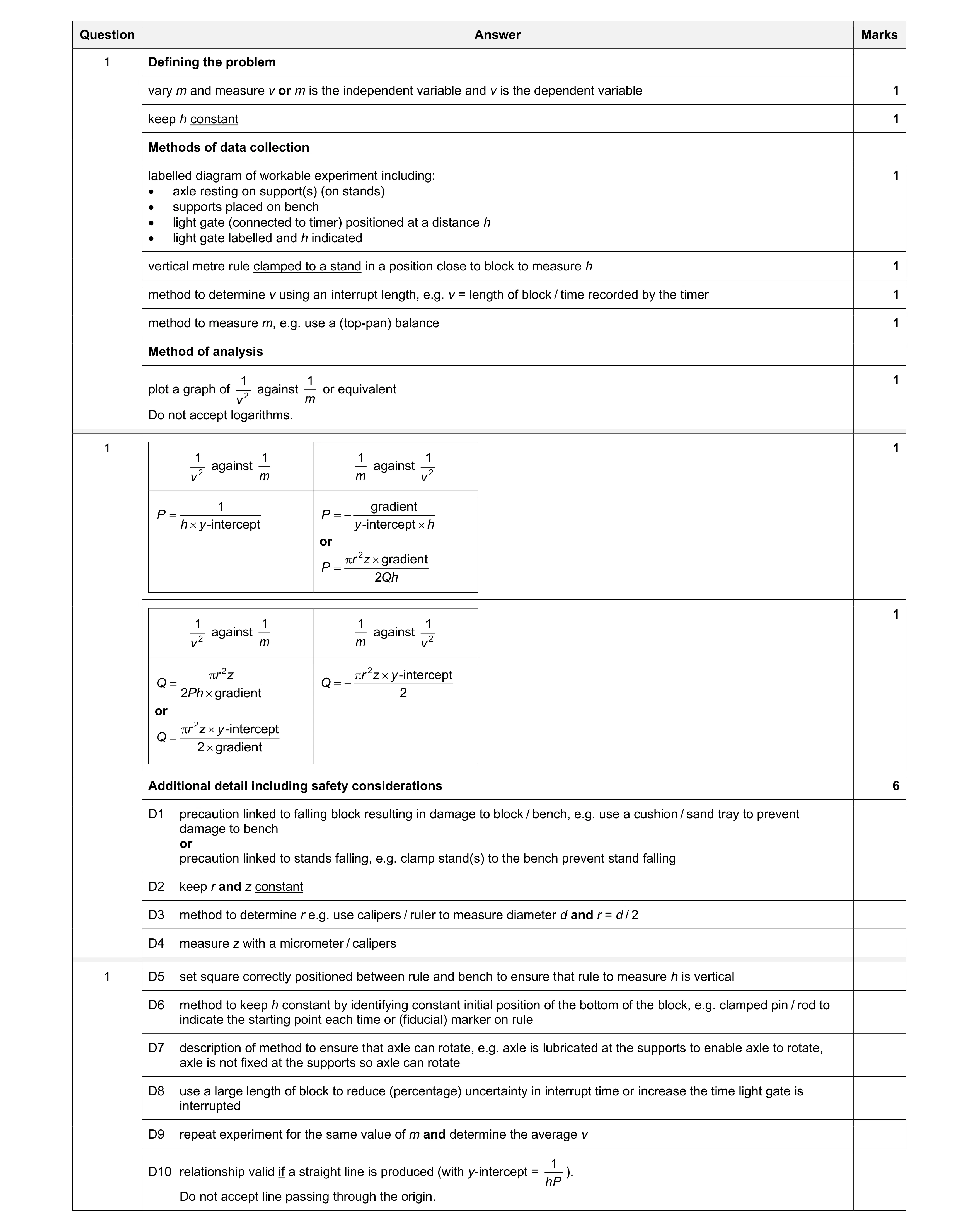 15
15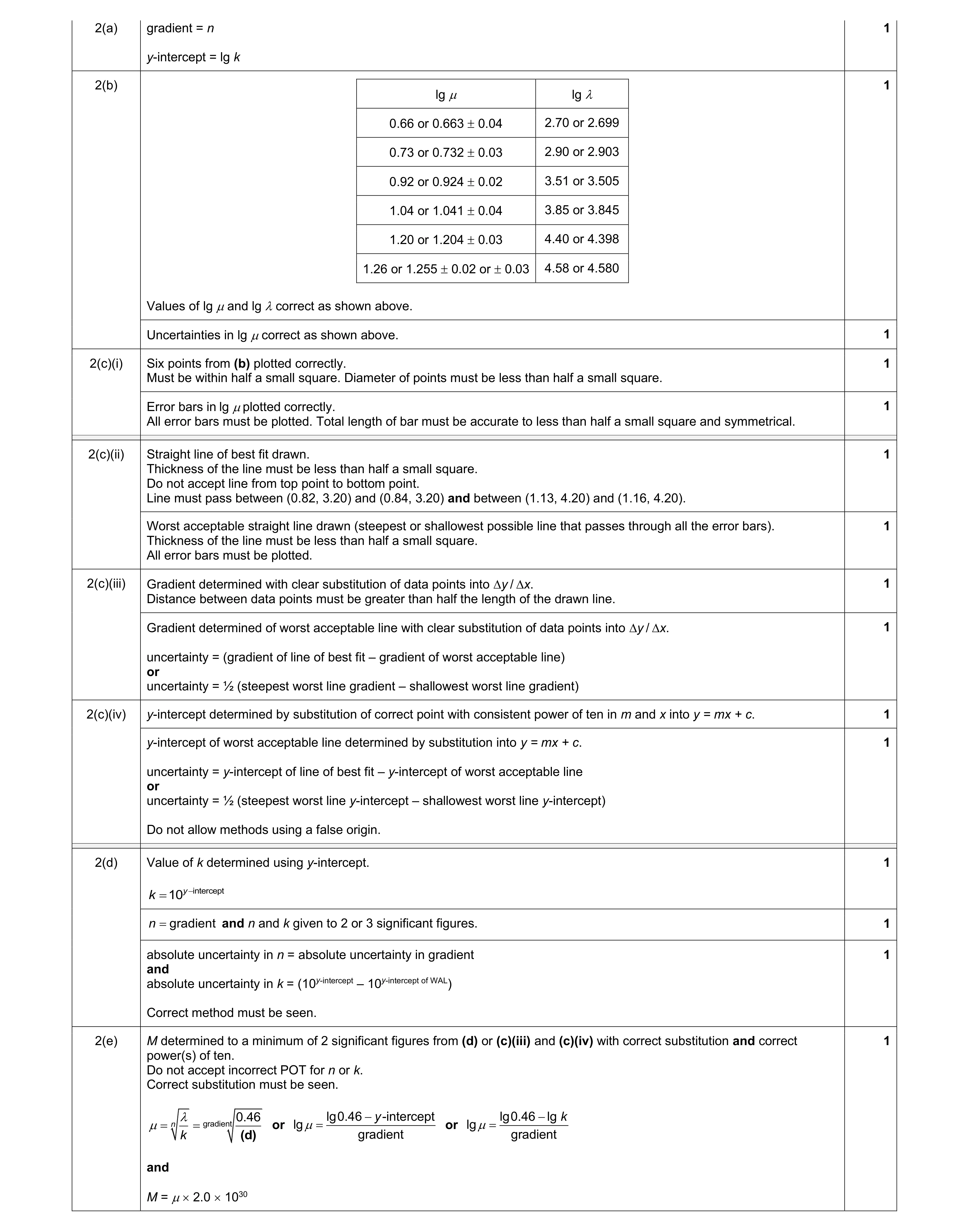 9
9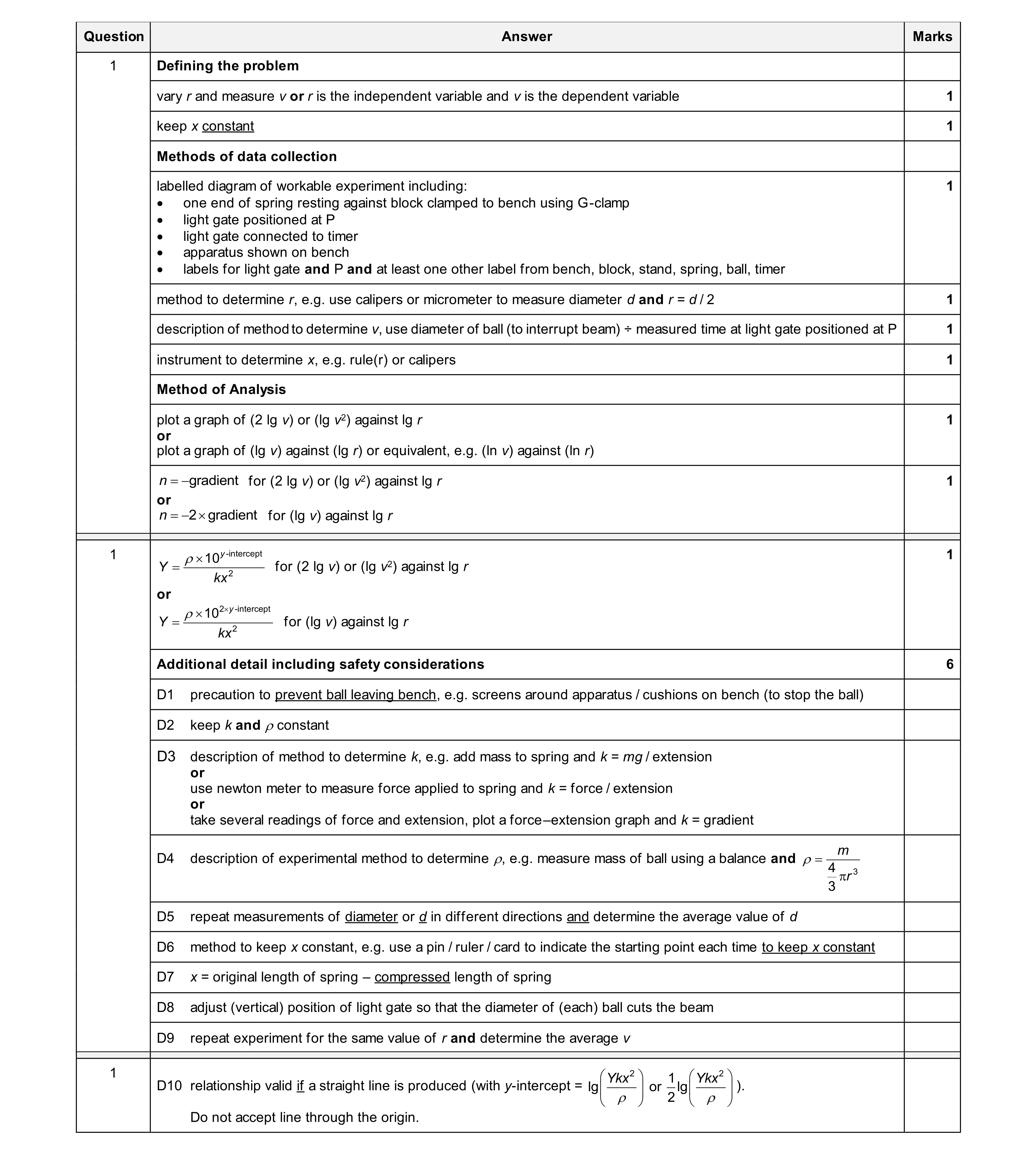 15
15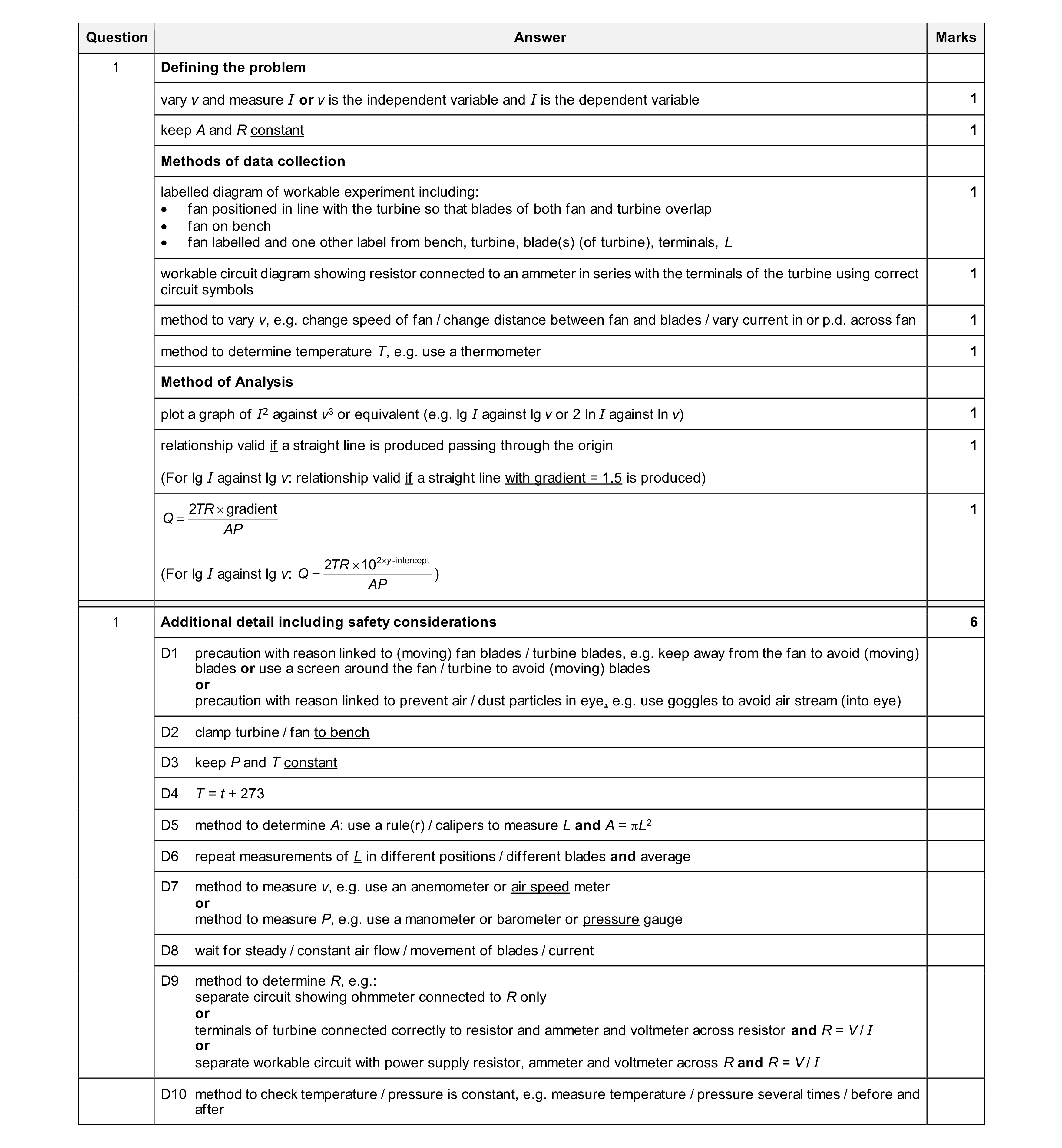 15
15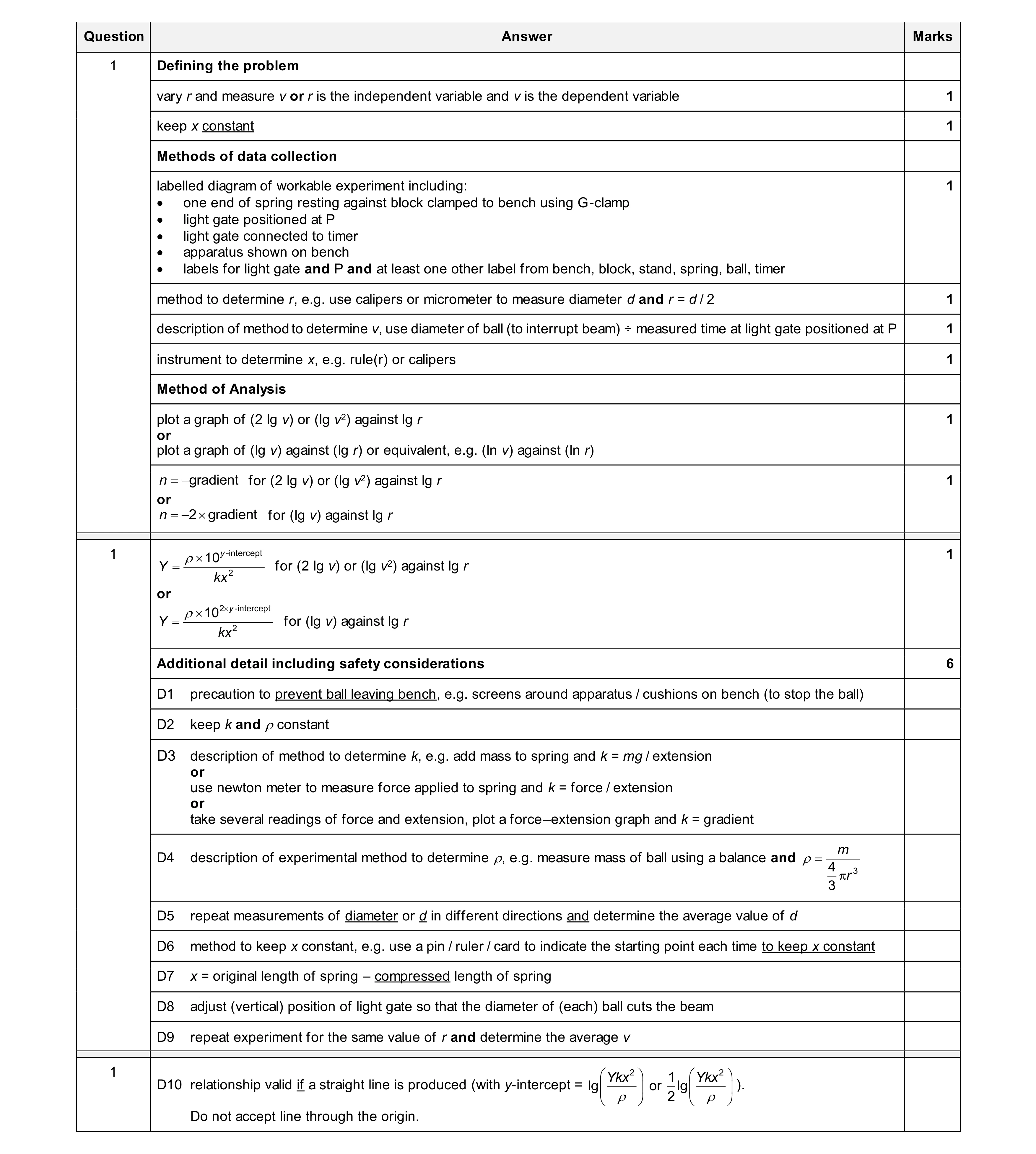 15
15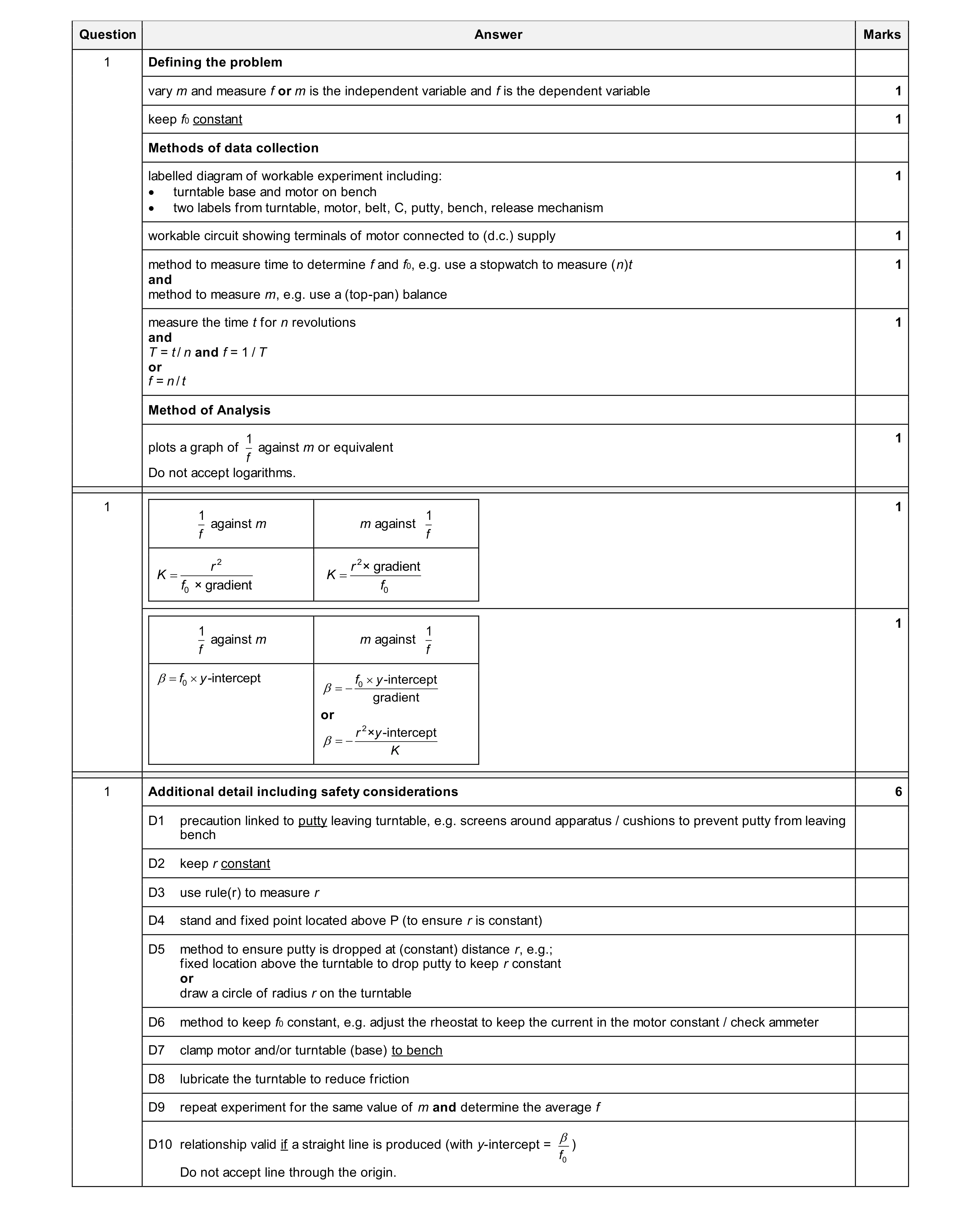 15
15