Questions as text
Q1 · Two randomly selected groups of students, with similar ranges of abilities, take the same… 9231/41 May/June 2020
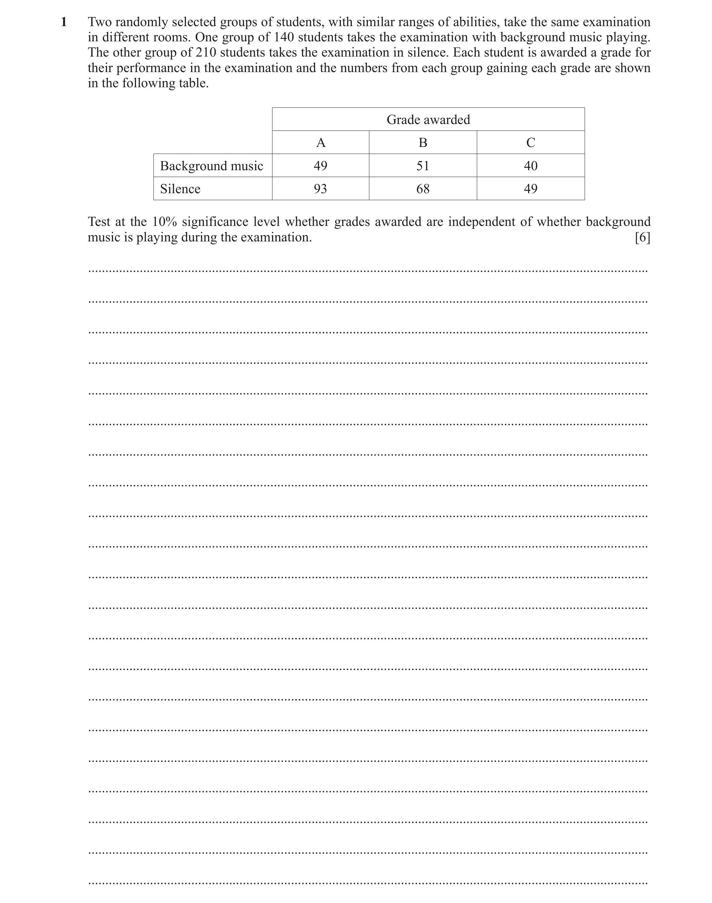
1 Two randomly selected groups of students, with similar ranges of abilities, take the same examination in different rooms. One group of 140 students takes the examination with background music playing. The other group of 210 students takes the examination in silence. Each student is awarded a grade for their performance in the examination and the numbers from each group gaining each grade are shown in the following table. Grade awarded A B C Background music 49 51 40 Silence 93 68 49 Test at the 10% significance level whether grades awarded are independent of whether background music is playing during the examination. [6] … … … … … … … … … … … … … … … … … … … … …
6 marks
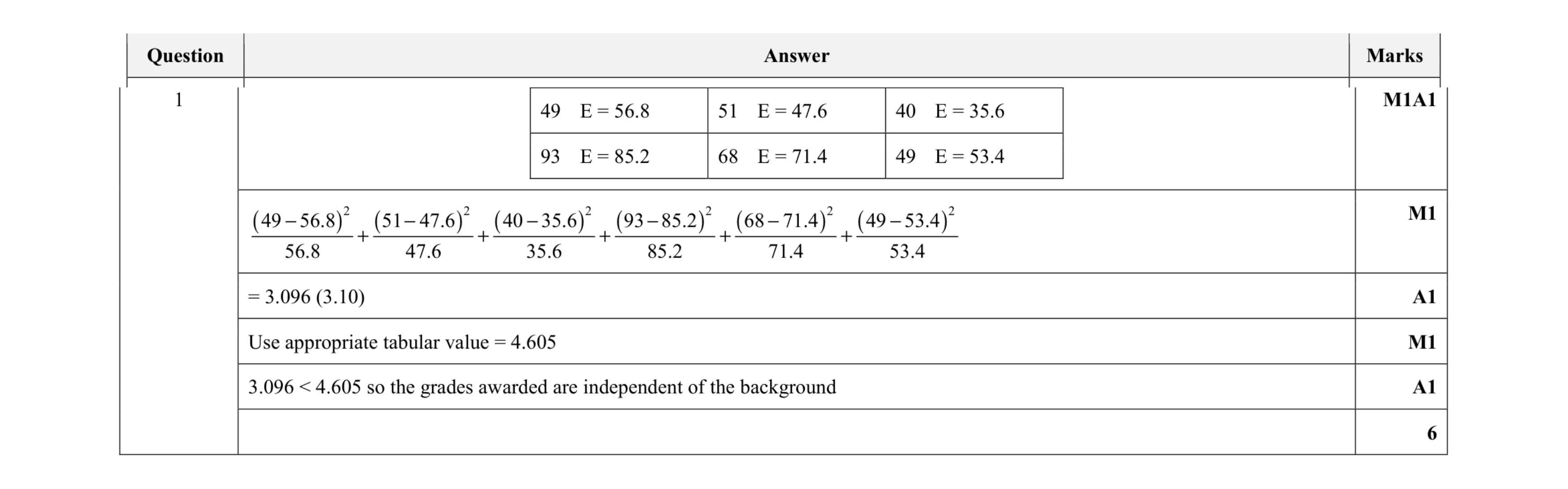
Mark scheme: 1 49 E = 56.8 51 E = 47.6 40 E = 35.6 93 E = 85.2 68 E = 71.4 49 E = 53.4 M1A1 ( ) ( ) ( ) ( ) ( ) ( ) 2 2 2 2 2 2 49 56.8 51 47.6 40 35.6 93 85.2 68 71.4 49 53.4 56.8 47.6 35.6 85.2 71.4 53.4 − − − − − − + + + + + M1 = 3.096 (3.10) A1 Use appropriate tabular value = 4.605 M1 3.096 < 4.605 so the grades awarded are independent of the background A1 6
This question in 9231/41 May/June 2020
Q2 · Two randomly selected groups of students, with similar ranges of abilities, take the same… 9231/42 May/June 2020
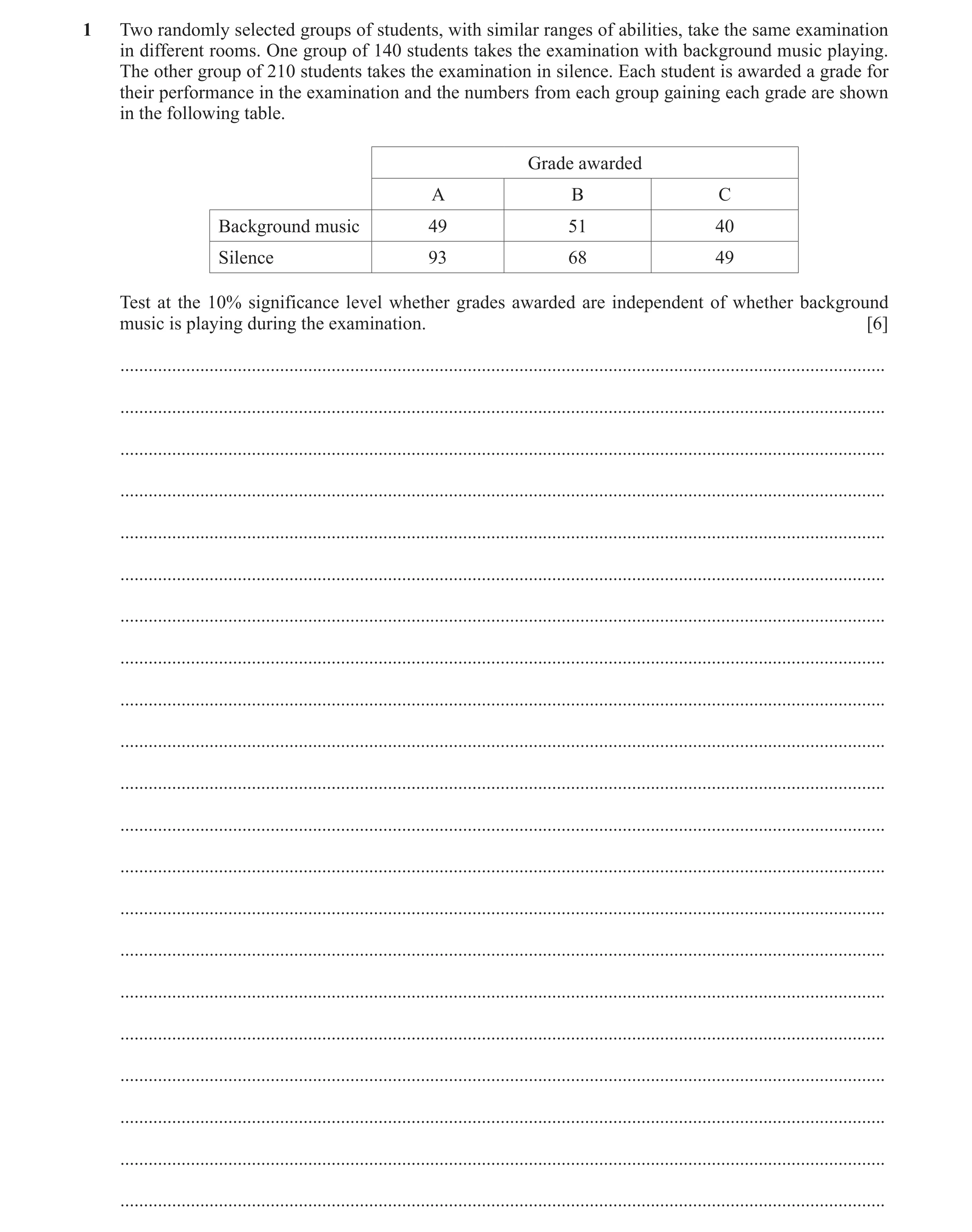
1 Two randomly selected groups of students, with similar ranges of abilities, take the same examination in different rooms. One group of 140 students takes the examination with background music playing. The other group of 210 students takes the examination in silence. Each student is awarded a grade for their performance in the examination and the numbers from each group gaining each grade are shown in the following table. Grade awarded A B C Background music 49 51 40 Silence 93 68 49 Test at the 10% significance level whether grades awarded are independent of whether background music is playing during the examination. [6] … … … … … … … … … … … … … … … … … … … … …
6 marks
Mark scheme: 1 49 E = 56.8 51 E = 47.6 40 E = 35.6 93 E = 85.2 68 E = 71.4 49 E = 53.4 M1A1 ( ) ( ) ( ) ( ) ( ) ( ) 2 2 2 2 2 2 49 56.8 51 47.6 40 35.6 93 85.2 68 71.4 49 53.4 56.8 47.6 35.6 85.2 71.4 53.4 − − − − − − + + + + + M1 = 3.096 (3.10) A1 Use appropriate tabular value = 4.605 M1 3.096 < 4.605 so the grades awarded are independent of the background A1 6
This question in 9231/42 May/June 2020
Q3 · Young children are learning to read using two different reading schemes, A and B 9231/43 May/June 2020
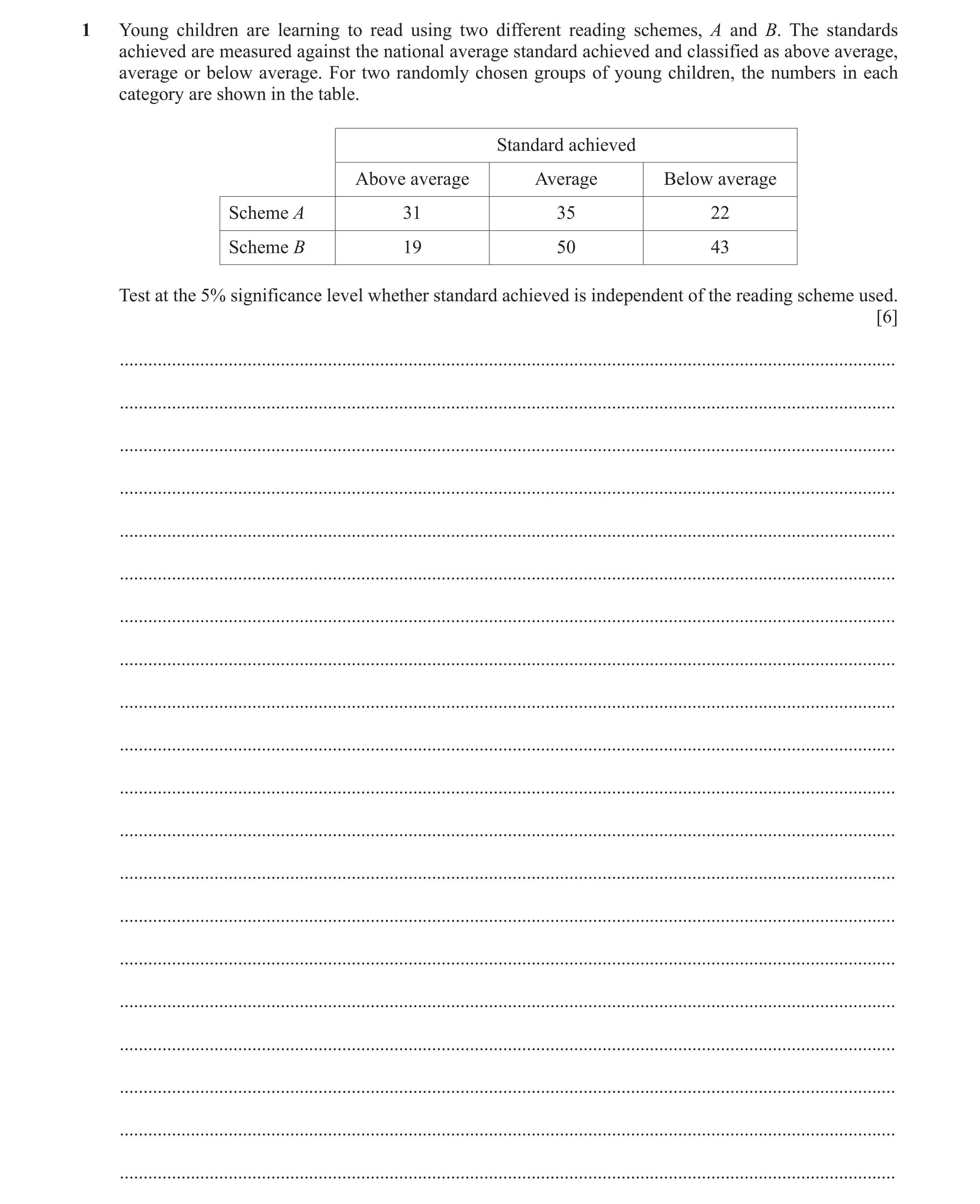
1 Young children are learning to read using two different reading schemes, A and B. The standards achieved are measured against the national average standard achieved and classified as above average, average or below average. For two randomly chosen groups of young children, the numbers in each category are shown in the table. Standard achieved Above average Average Below average Scheme A 31 35 22 Scheme B 19 50 43 Test at the 5% significance level whether standard achieved is independent of the reading scheme used. [6] … … … … … … … … … … … … … … … … … … … …
6 marks
Mark scheme: 1 31 E = 22 35 E = 37.4 22 E = 28.6 19 E = 28 50 E = 47.6 43 E = 36.4 M1A1 ( ) ( ) ( ) ( ) ( ) ( ) 2 2 2 2 2 2 31 22 35 37.4 22 28.6 19 28 50 47.6 43 36.4 22 37.4 28.6 28 47.6 36.4 − − − − − − + + + + + M1 9.569 (9.57) A1 Tabular value = 5.991 and comparing 9.569 > 5.991 M1 So standard achieved is dependent on reading scheme used A1 6
This question in 9231/43 May/June 2020
Q4 · Apples are sold in bags of 5 9231/41 Oct/Nov 2020
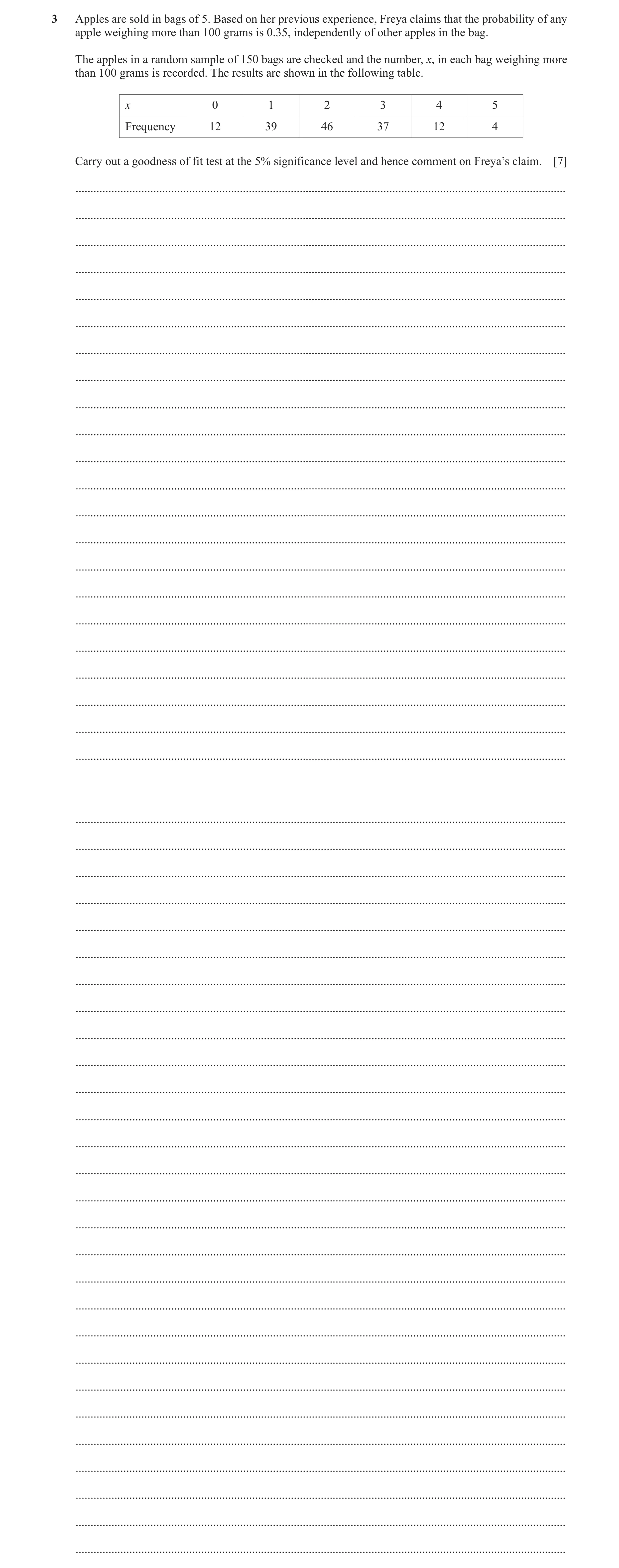
3 Apples are sold in bags of 5. Based on her previous experience, Freya claims that the probability of any apple weighing more than 100 grams is 0.35, independently of other apples in the bag. The apples in a random sample of 150 bags are checked and the number, x, in each bag weighing more than 100 grams is recorded. The results are shown in the following table. x 0 1 2 3 4 5 Frequency 12 39 46 37 12 4 Carry out a goodness of fit test at the 5% significance level and hence comment on Freya’s claim. [7] … … … … … … … … … … … … … … … … … … … … … … … … … … … … … … … … … … … … … … … … … … … … … … … … … …
7 marks
Mark scheme: 3 x 0 1 2 3 4 5 Observed freq 12 39 46 37 12 4 Bin prob 0.11603 0.31236 0.33642 0.18115 0.04877 0.00525 Expected freq 17.404 46.858 50.462 27.172 7.316 0.7878 M1 A1 Attempt at E values (at least 4 correct) All correct, to 2 dp or better Add last two columns: 16, 8.104 M1 ( ) ( ) ( ) 2 2 2 17.404 12 46.858 39 50.462 46 17.404 46.858 50.462 − − − + + + ( ) ( ) 2 2 27.172 37 8.104 16 27.172 8.104 − − + = 14.64 or 14.65 M1 A1 Accept 14.6 – 14.7 ’14.64’ > 9.49 M1 Compare their value with 9.49 Freya’s claim is not supported or Data does not fit the distribution A1 FT Correct conclusion in context, FT only their 14.64 SC for Poisson M0M1M1M0 max 2 7
This question in 9231/41 Oct/Nov 2020
Q5 · A random sample of 200 observations of the continuous random variable X was taken and the… 9231/42 Oct/Nov 2020
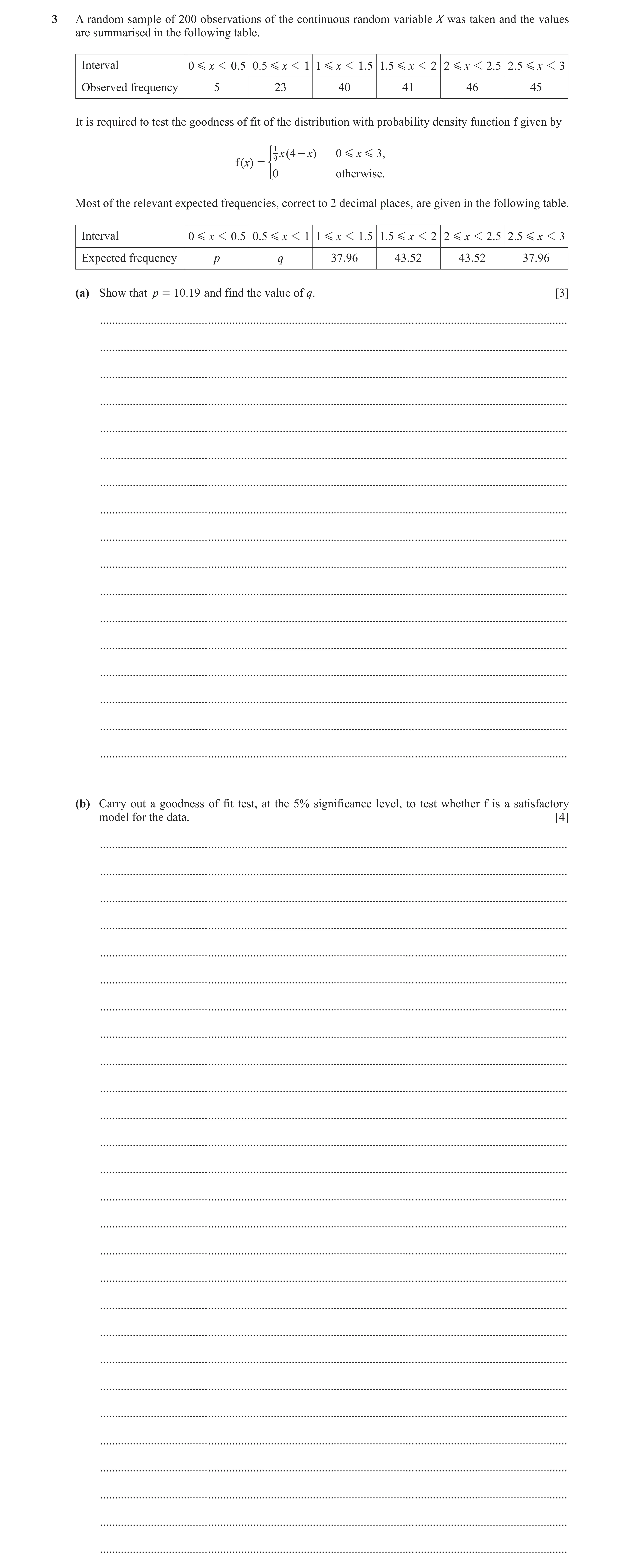
3 A random sample of 200 observations of the continuous random variable X was taken and the values are summarised in the following table. Interval 0 G x 1 0.5 0.5 G x 1 1 1 G x 1 1.5 1.5 G x 1 2 2 G x 1 2.5 2.5 G x 1 3 Observed frequency 5 23 40 41 46 45 It is required to test the goodness of fit of the distribution with probability density function f given by 1 9 x ( 4 - x) 0 G x G 3, f ( x) = *0 otherwise. Most of the relevant expected frequencies, correct to 2 decimal places, are given in the following table. Interval 0 G x 1 0 .5 0.5 G x 1 1 1 G x 1 1.5 1.5 G x 1 2 2 G x 1 2.5 2.5 G x 1 3 Expected frequency p q 37.96 43.52 43.52 37.96 (a) Show that p = 10.19 and find the value of q. [3] … … … … … … … … … … … … … … … … … (b) Carry out a goodness of fit test, at the 5% significance level, to test whether f is a satisfactory model for the data. [4] … … … … … … … … … … … … … … … … … … … … … … … … … … …
7 marks
Mark scheme: 3(a) 0.5 2 0 4 1 d [ 9 9 x x x − = 2 3 1 1 2 0.5 0.5 9 3 × − ] (= 0.0509(26) or 11 216 ) M1 Statement of integration with correct limits Freq = p = 0.0509(26) × 200 = 10.19 AG A1 Requires sight of 0.0509 or 11 216 By addition to 200, q = 26.85 725 27 B1 Or by integration 3 3(b) O 5 23 40 41 46 45 E 10.19 26.85 37.96 43.52 43.52 37.96 Test statistic = 2.6433 + 0.5520 + 0.1096 + 0.1459 + 0.1413 + 1.3056 M1 At least 4 correct 4.89 or 4.90 A1 ‘4.90’ < 11.07: M1 Compare their value with 11.07 PDF is a satisfactory model for the data. A1 FT Correct conclusion in context, ft only their 4.90 4
This question in 9231/42 Oct/Nov 2020
Q6 · Apples are sold in bags of 5 9231/43 Oct/Nov 2020
3 Apples are sold in bags of 5. Based on her previous experience, Freya claims that the probability of any apple weighing more than 100 grams is 0.35, independently of other apples in the bag. The apples in a random sample of 150 bags are checked and the number, x, in each bag weighing more than 100 grams is recorded. The results are shown in the following table. x 0 1 2 3 4 5 Frequency 12 39 46 37 12 4 Carry out a goodness of fit test at the 5% significance level and hence comment on Freya’s claim. [7] … … … … … … … … … … … … … … … … … … … … … … … … … … … … … … … … … … … … … … … … … … … … … … … … … …
7 marks
Mark scheme: 3 x 0 1 2 3 4 5 Observed freq 12 39 46 37 12 4 Bin prob 0.11603 0.31236 0.33642 0.18115 0.04877 0.00525 Expected freq 17.404 46.858 50.462 27.172 7.316 0.7878 M1 A1 Attempt at E values (at least 4 correct) All correct, to 2 dp or better Add last two columns: 16, 8.104 M1 ( ) ( ) ( ) 2 2 2 17.404 12 46.858 39 50.462 46 17.404 46.858 50.462 − − − + + + ( ) ( ) 2 2 27.172 37 8.104 16 27.172 8.104 − − + = 14.64 or 14.65 M1 A1 Accept 14.6 – 14.7 ’14.64’ > 9.49 M1 Compare their value with 9.49 Freya’s claim is not supported or Data does not fit the distribution A1 FT Correct conclusion in context, FT only their 14.64 SC for Poisson M0M1M1M0 max 2 7
This question in 9231/43 Oct/Nov 2020
Q7 · A driving school employs four instructors to prepare people for their driving test 9231/41 May/June 2021
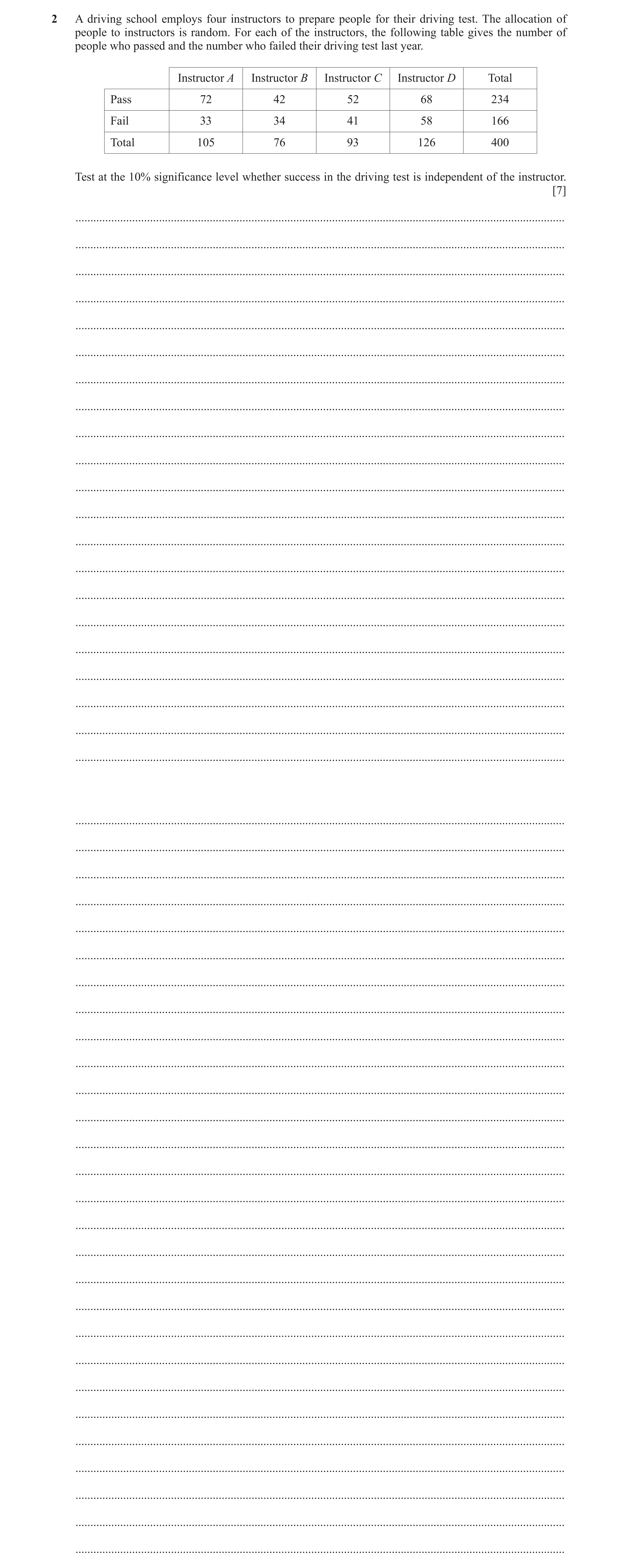
2 A driving school employs four instructors to prepare people for their driving test. The allocation of people to instructors is random. For each of the instructors, the following table gives the number of people who passed and the number who failed their driving test last year. Instructor A Instructor B Instructor C Instructor D Total Pass 72 42 52 68 234 Fail 33 34 41 58 166 Total 105 76 93 126 400 Test at the 10% significance level whether success in the driving test is independent of the instructor. [7] … … … … … … … … … … … … … … … … … … … … … … … … … … … … … … … … … … … … … … … … … … … … … … … … …
7 marks
Mark scheme: 2 72 (61.425) 42 (44.46) 52 (54.405) 68 (73.71) 33 (43.575) 34 (31.54) 41 (38.595) 58 (52.29) M1 At least 3 correct to 4sf. Calculates E values (in brackets above) A1 All correct to 4sf (if 6.037 not found). Test value: ( ) 2 O E E − = 1.8206 + 0.1361 + 0.1063 +0.4423 + 2.5664 + 0.1919 + 0.1499 + 0.6235 M1 Correct formula used. = 6.037 A1 Correct to 3 sf. H0: (driving) test success is independent of instructor B1 Tabular value: 3 df 10% = 6.251 6.04 < 6.251 Accept 0 H M1 Compare with correct tabular value and conclusion. Sufficient evidence to suggest that (driving) test success is independent of instructor A1 Correct conclusion, in context, following correct work. Level of uncertainty in language is used. Allow ±1 in the third significant figure of test value. 7
This question in 9231/41 May/June 2021
Q8 · A driving school employs four instructors to prepare people for their driving test 9231/42 May/June 2021
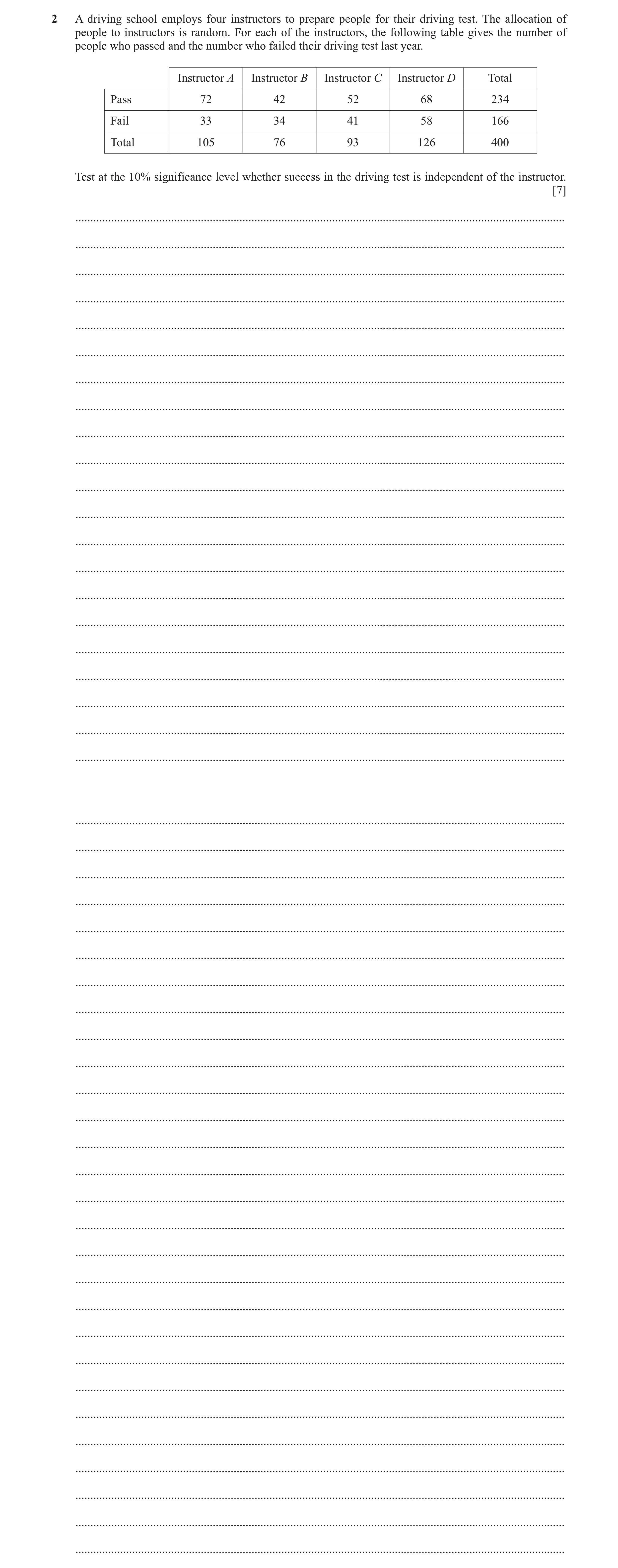
2 A driving school employs four instructors to prepare people for their driving test. The allocation of people to instructors is random. For each of the instructors, the following table gives the number of people who passed and the number who failed their driving test last year. Instructor A Instructor B Instructor C Instructor D Total Pass 72 42 52 68 234 Fail 33 34 41 58 166 Total 105 76 93 126 400 Test at the 10% significance level whether success in the driving test is independent of the instructor. [7] … … … … … … … … … … … … … … … … … … … … … … … … … … … … … … … … … … … … … … … … … … … … … … … … …
7 marks
Mark scheme: 2 72 (61.425) 42 (44.46) 52 (54.405) 68 (73.71) 33 (43.575) 34 (31.54) 41 (38.595) 58 (52.29) M1 At least 3 correct to 4sf. Calculates E values (in brackets above) A1 All correct to 4sf (if 6.037 not found). Test value: ( ) 2 O E E − = 1.8206 + 0.1361 + 0.1063 +0.4423 + 2.5664 + 0.1919 + 0.1499 + 0.6235 M1 Correct formula used. = 6.037 A1 Correct to 3 sf. H0: (driving) test success is independent of instructor B1 Tabular value: 3 df 10% = 6.251 6.04 < 6.251 Accept 0 H M1 Compare with correct tabular value and conclusion. Sufficient evidence to suggest that (driving) test success is independent of instructor A1 Correct conclusion, in context, following correct work. Level of uncertainty in language is used. Allow ±1 in the third significant figure of test value. 7
This question in 9231/42 May/June 2021
Q9 · Chai packs china mugs into cardboard boxes 9231/43 May/June 2021
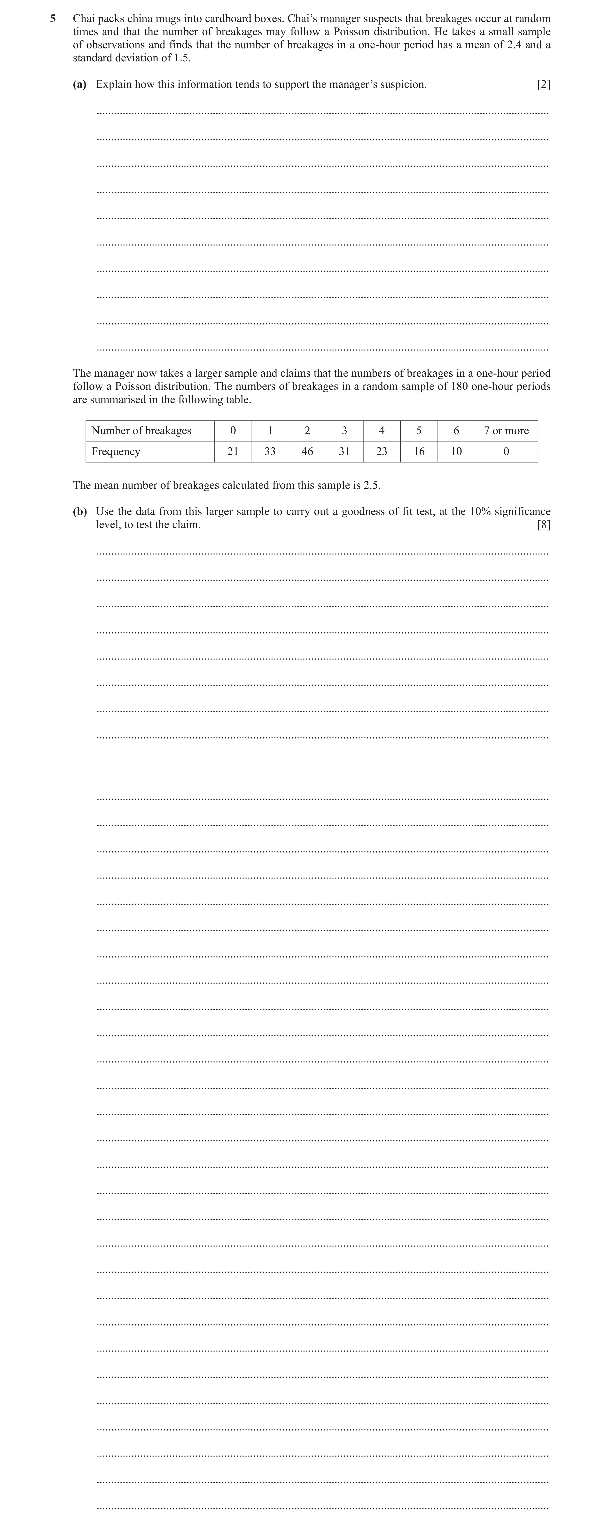
5 Chai packs china mugs into cardboard boxes. Chai’s manager suspects that breakages occur at random times and that the number of breakages may follow a Poisson distribution. He takes a small sample of observations and finds that the number of breakages in a one-hour period has a mean of 2.4 and a standard deviation of 1.5. (a) Explain how this information tends to support the manager’s suspicion. [2] … … … … … … … … … … The manager now takes a larger sample and claims that the numbers of breakages in a one-hour period follow a Poisson distribution. The numbers of breakages in a random sample of 180 one-hour periods are summarised in the following table. Number of breakages 0 1 2 3 4 5 6 7 or more Frequency 21 33 46 31 23 16 10 0 The mean number of breakages calculated from this sample is 2.5. (b) Use the data from this larger sample to carry out a goodness of fit test, at the 10% significance level, to test the claim. [8] … … … … … … … … … … … … … … … … … … … … … … … … … … … … … … … … … … … …
10 marks
Mark scheme: 5(a) (Mean of distribution = 2.4) Variance = 2.25 Mean approx. equal to variance (so Poisson might be suitable) A1 Must have ‘approximately’ oe, not equality. Must have 2.25. 2 5(b) Po(2.5) leads to frequencies: M1 At least 3 correct to 3sf. 14.77[5], 36.938, 46.173, 38.477, 24.048, 12.024, 5.010, 2.554 A1 All correct to 4sf. Combine last two values: 7.564 M1 FT their table values if final figure is less than 5. ( ) 2 2.6227 0.4198 0.00065 1.4529 0.04570 O E E − = + + + + 1.3148 0.7845 + + M1 Apply correct formula to their frequencies. 6.64 A1 Correct to 3sf. 5(b) H0: distribution fits the data B1 Must mention data and distribution . Tabular value, 5 degrees of freedom, is 9.236 ‘6.64’ < 9.236, so accept H0 M1 Compare with correct tabular value and conclusion. Insufficient evidence to show that data does not follow a Poisson distribution A1 Correct conclusion, in context, following correct work. Level of uncertainty in language is used. Allow ±1 difference in third significant figure. 8
This question in 9231/43 May/June 2021
Q10 · A supermarket sells pears in packs of 8 9231/41 Oct/Nov 2021
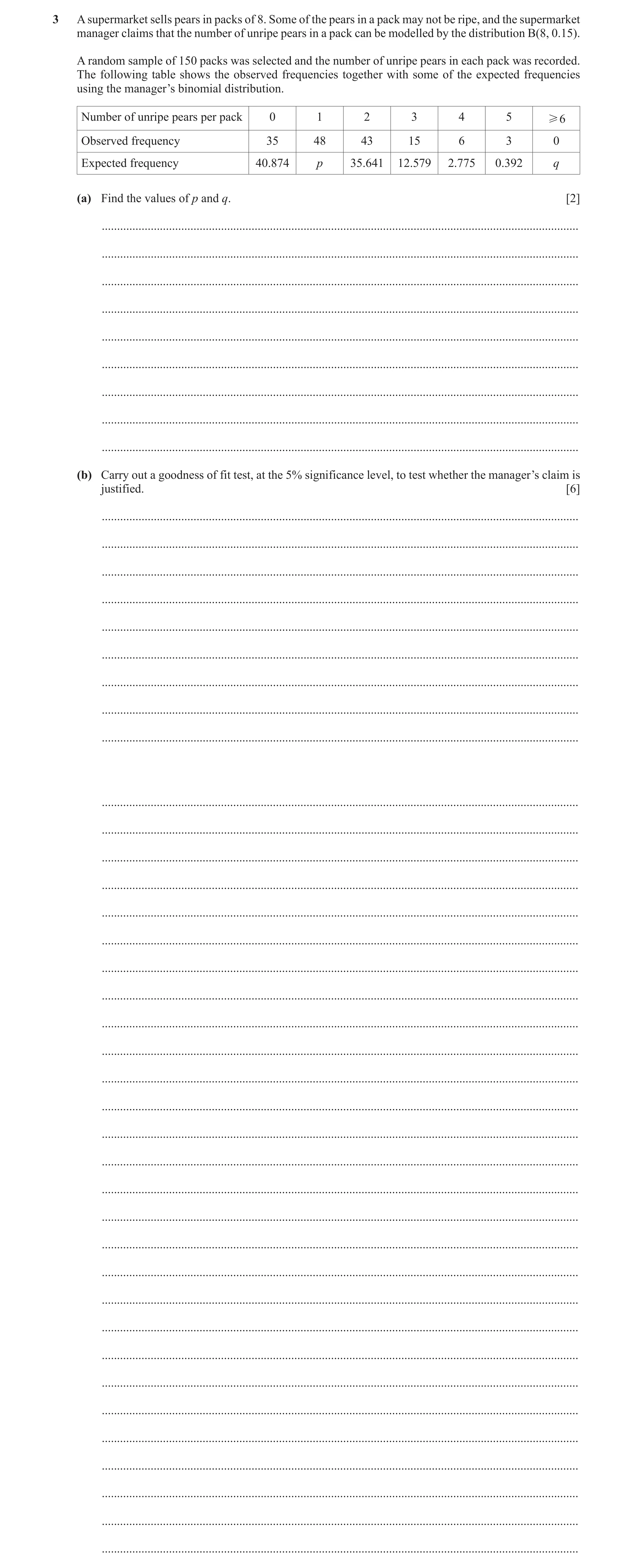
3 A supermarket sells pears in packs of 8. Some of the pears in a pack may not be ripe, and the supermarket manager claims that the number of unripe pears in a pack can be modelled by the distribution B(8, 0.15). A random sample of 150 packs was selected and the number of unripe pears in each pack was recorded. The following table shows the observed frequencies together with some of the expected frequencies using the manager’s binomial distribution. Number of unripe pears per pack 0 1 2 3 4 5 H6 Observed frequency 35 48 43 15 6 3 0 Expected frequency 40.874 p 35.641 12.579 2.775 0.392 q (a) Find the values of p and q. [2] … … … … … … … … … (b) Carry out a goodness of fit test, at the 5% significance level, to test whether the manager’s claim is justified. [6] … … … … … … … … … … … … … … … … … … … … … … … … … … … … … … … … … … … … …
8 marks
Mark scheme: 3(a) x 0 1 2 3 4 5 6 or more O 35 48 43 15 6 3 0 E 40.874 57.704 35.641 12.579 2.775 0.392 0.0352 p = 57.704 B1 3 dp or better. q = 0.035 or 0.036 B1 Accept numbers which round to 0.035 or 0.036. 2 Question Answer Marks Guidance 3(b) Combine frequencies less than 5: last 4 columns give 24 / 15.7812 M1 Allow last 2 or 3 columns combined for this M1. ( ) 2 0.8444 1.6319 1.5199 4.2803 O E E − = + + + M1 8.28 A1 Accept 8.27 – 8.28. SC: 25.60, if values not combined, scores M1A0. SC: 14.96 if last 3 combined, scores M1A0. SC: if last 2 combined, scores M1A0. H0: B(8, 0.15) fits the data B1 Must mention distribution and data. 3 degrees of freedom, tabular value = 7.815. 8.28 > 7.815 Reject 0 H . M1 Compare their value with 7.815 and correct FT conclusion 3 columns combined compared with 9.488 and correct conclusion Insufficient evidence to support manager’s claim. A1 Correct conclusion, in context, following correct work. Level of uncertainty in language is used. 6
This question in 9231/41 Oct/Nov 2021
Q11 · It is claimed that the heights of a particular age group of boys follow a normal… 9231/42 Oct/Nov 2021
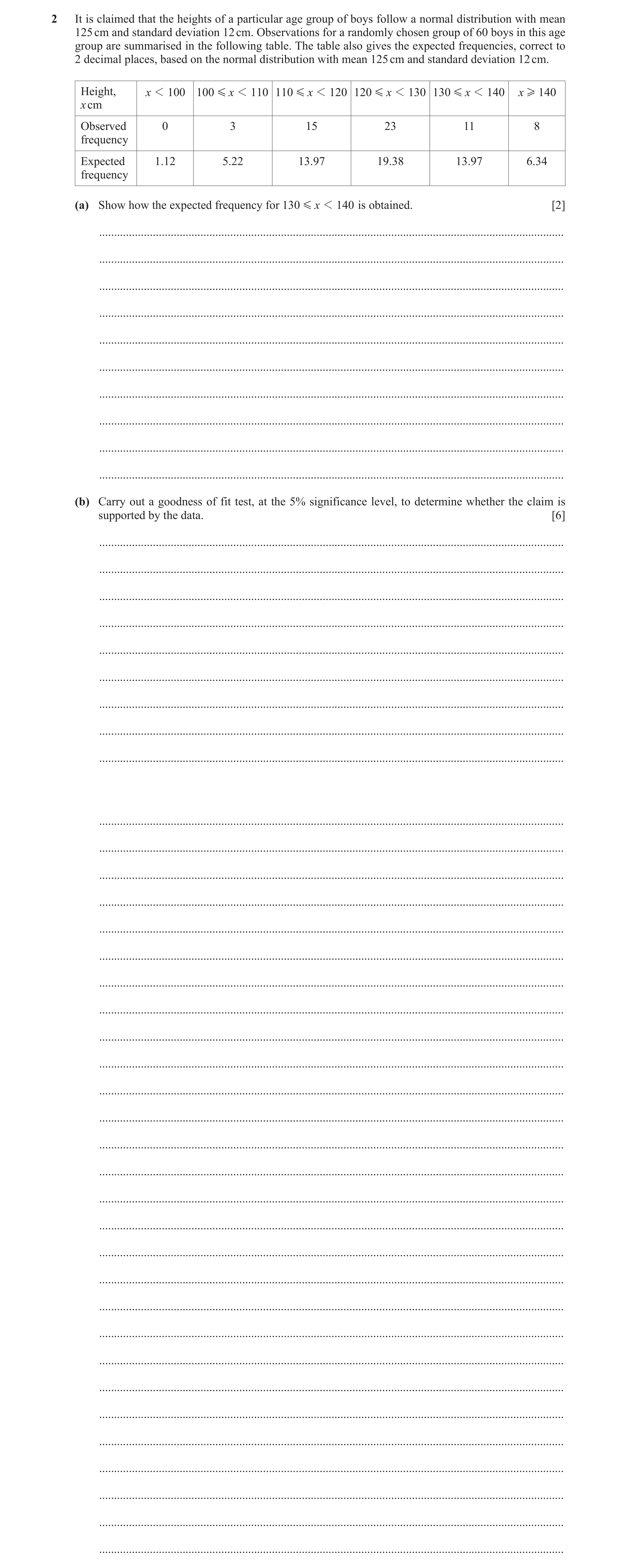
2 It is claimed that the heights of a particular age group of boys follow a normal distribution with mean 125 cm and standard deviation 12 cm. Observations for a randomly chosen group of 60 boys in this age group are summarised in the following table. The table also gives the expected frequencies, correct to 2 decimal places, based on the normal distribution with mean 125 cm and standard deviation 12 cm. Height, x 1 100 100 G x 1 110 110 G x 1 120 120 G x 1 130 130 G x 1 140 x H 140 x cm Observed 0 3 15 23 11 8 frequency Expected 1.12 5.22 13.97 19.38 13.97 6.34 frequency (a) Show how the expected frequency for 130 G x 1 140 is obtained. [2] … … … … … … … … … … (b) Carry out a goodness of fit test, at the 5% significance level, to determine whether the claim is supported by the data. [6] … … … … … … … … … … … … … … … … … … … … … … … … … … … … … … … … … … … … …
8 marks
Mark scheme: 2(a) P(130 140 < x ) = P 130 125 140 125 12 12 Z − − < ≤ P( 0.4167 1.25) < < Z Must see 0.4167 and 1.25, may be implied by 0.8944 and 0.6616 Accept 0.417. 0.8944 0.6616 0.2328 − = Multiply by 60 leads to 13.97 A1 AG Accept 0.6615. Need to see 0.2328 or 0.2329 or 13.968 or ( ) 0.8944 0.6616 60 − × . 2 2(b) 0 3 15 23 11 8 1.12 5.22 13.97 19.38 13.97 6.34 M1 Combine first two values. Test stat = 1.7588 + 0.0761 + 0.6743 + 0.6309 + 0.4352 M1 3.58 A1 Accept 3.57 – 3.58 . SC: 3.88, if values not combined, scores M1A0. 0 : distribution fits data H N(125, 122) is a good model for the data oe B1 Must mention distribution and data. 4 degrees of freedom, so tabular value = 9.488 3.58 < 9.488 Accept 0 H . M1 Compare their value with 9.488 (9.49) and correct FT conclusion. Or, if values not combined, compare their value with 11.07 and correct FT conclusion for M1A0. There is sufficient evidence that the normal distribution fits the data There is sufficient evidence that the claim is supported by the data A1 Correct conclusion, in context, following correct work. Level of uncertainty in language is used. 6
This question in 9231/42 Oct/Nov 2021
Q12 · A supermarket sells pears in packs of 8 9231/43 Oct/Nov 2021
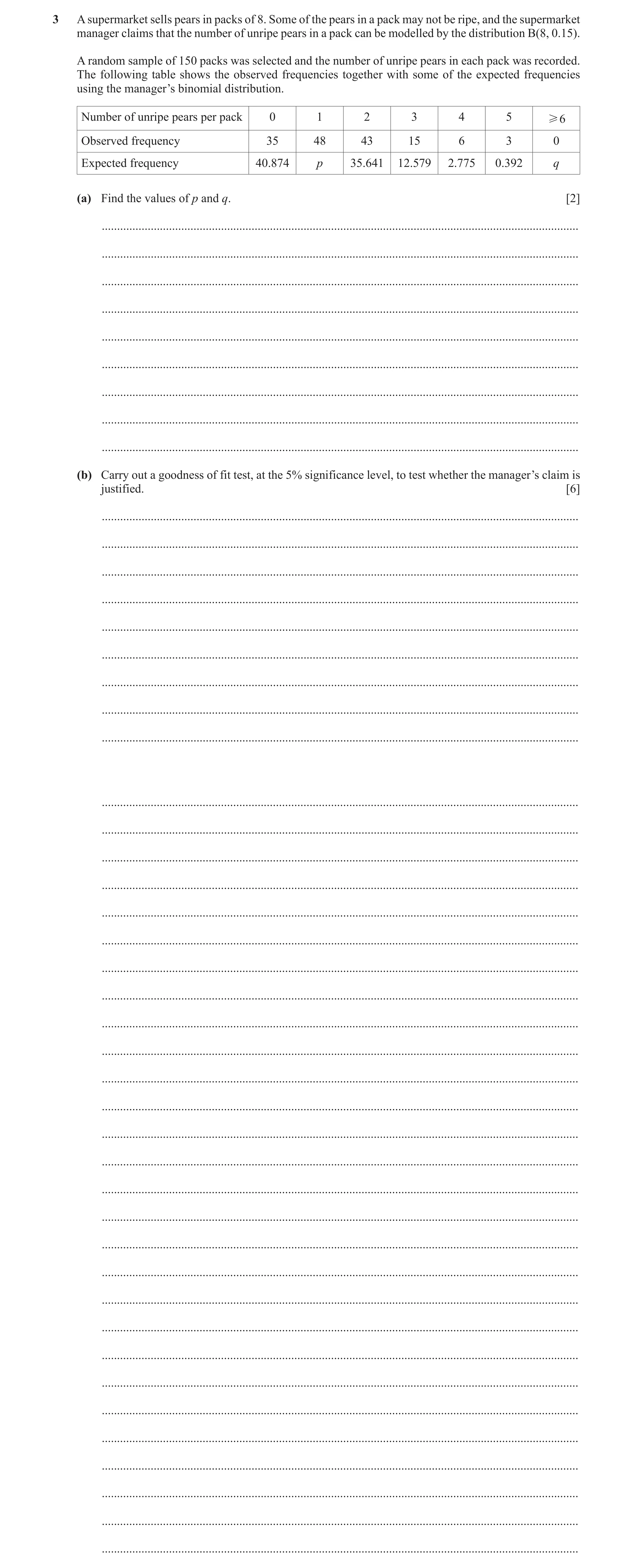
3 A supermarket sells pears in packs of 8. Some of the pears in a pack may not be ripe, and the supermarket manager claims that the number of unripe pears in a pack can be modelled by the distribution B(8, 0.15). A random sample of 150 packs was selected and the number of unripe pears in each pack was recorded. The following table shows the observed frequencies together with some of the expected frequencies using the manager’s binomial distribution. Number of unripe pears per pack 0 1 2 3 4 5 H6 Observed frequency 35 48 43 15 6 3 0 Expected frequency 40.874 p 35.641 12.579 2.775 0.392 q (a) Find the values of p and q. [2] … … … … … … … … … (b) Carry out a goodness of fit test, at the 5% significance level, to test whether the manager’s claim is justified. [6] … … … … … … … … … … … … … … … … … … … … … … … … … … … … … … … … … … … … …
8 marks
Mark scheme: 3(a) x 0 1 2 3 4 5 6 or more O 35 48 43 15 6 3 0 E 40.874 57.704 35.641 12.579 2.775 0.392 0.0352 p = 57.704 B1 3 dp or better. q = 0.035 or 0.036 B1 Accept numbers which round to 0.035 or 0.036. 2 Question Answer Marks Guidance 3(b) Combine frequencies less than 5: last 4 columns give 24 / 15.7812 M1 Allow last 2 or 3 columns combined for this M1. ( ) 2 0.8444 1.6319 1.5199 4.2803 O E E − = + + + M1 8.28 A1 Accept 8.27 – 8.28. SC: 25.60, if values not combined, scores M1A0. SC: 14.96 if last 3 combined, scores M1A0. SC: if last 2 combined, scores M1A0. H0: B(8, 0.15) fits the data B1 Must mention distribution and data. 3 degrees of freedom, tabular value = 7.815. 8.28 > 7.815 Reject 0 H . M1 Compare their value with 7.815 and correct FT conclusion 3 columns combined compared with 9.488 and correct conclusion Insufficient evidence to support manager’s claim. A1 Correct conclusion, in context, following correct work. Level of uncertainty in language is used. 6
This question in 9231/43 Oct/Nov 2021
Q13 · A scientist is investigating the numbers of a particular type of butterfly in a certain… 9231/41 May/June 2022
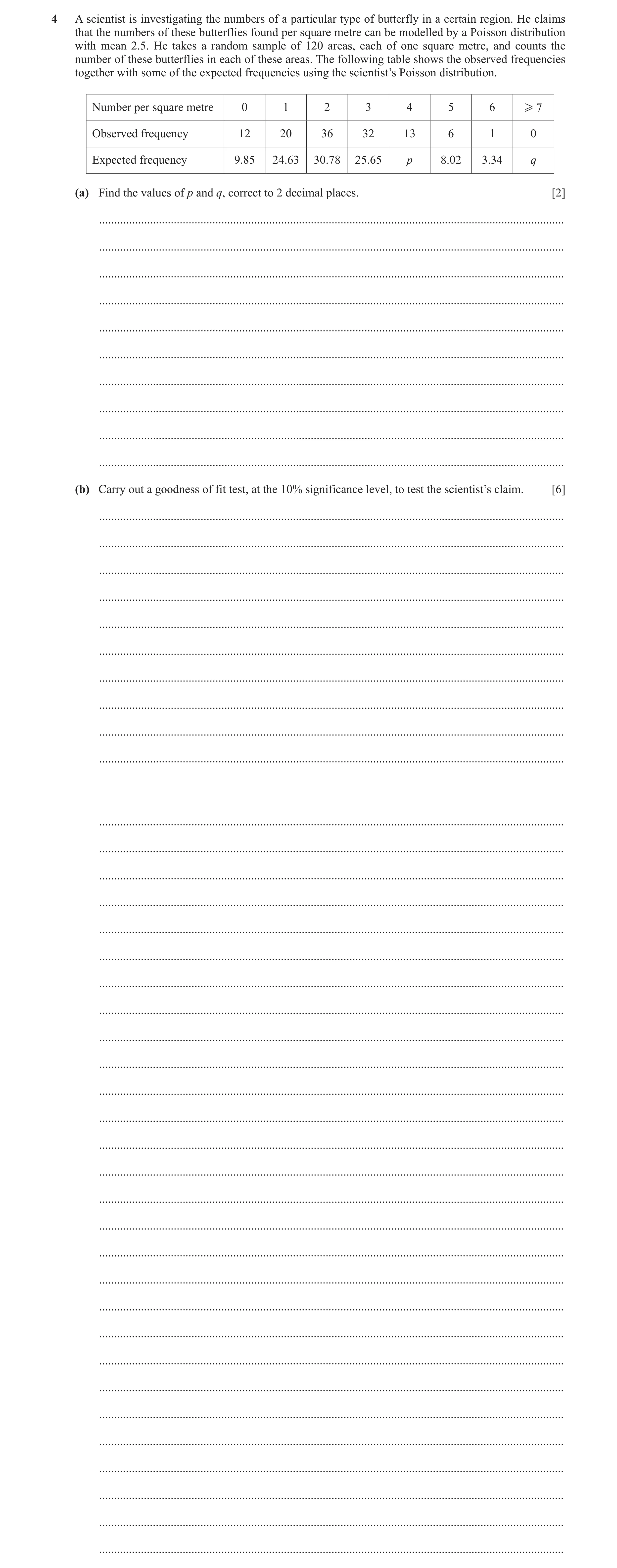
4 A scientist is investigating the numbers of a particular type of butterfly in a certain region. He claims that the numbers of these butterflies found per square metre can be modelled by a Poisson distribution with mean 2.5. He takes a random sample of 120 areas, each of one square metre, and counts the number of these butterflies in each of these areas. The following table shows the observed frequencies together with some of the expected frequencies using the scientist’s Poisson distribution. Number per square metre 0 1 2 3 4 5 6 H 7 Observed frequency 12 20 36 32 13 6 1 0 Expected frequency 9.85 24.63 30.78 25.65 p 8.02 3.34 q (a) Find the values of p and q, correct to 2 decimal places. [2] … … … … … … … … … … (b) Carry out a goodness of fit test, at the 10% significance level, to test the scientist’s claim. [6] … … … … … … … … … … … … … … … … … … … … … … … … … … … … … … … … … … … … … …
8 marks
Mark scheme: 4(a) 1.70 q B1 Condone 1.7 2 Question Answer Marks Guidance 4(b) 0 1 2 3 4 5 6 7 12 20 36 32 13 6 1 0 9.85 24.63 30.78 25.65 16.03 8.02 3.34 1.70 Combine last two columns: O value = 1, E value = 5.04 M1 Add last 2 columns (or 3 columns: 13.06). Calculate values of 2 O E E : 0.4693 0.8704 0.8853 1.5720 0.5727 0.5088 3.2384 M1 Calculate values. Test statistic = 8.12 A1 H0: data fits a Poisson distribution with mean 2.5 H1: data does not fit a Poisson distribution with mean 2.5 B1 Need data and distribution. e.g Data fits the given distribution. Number of butterflies per square metre fits Po(2.5). Critical value of chi-squared = 10.64 Compare: ‘8.12’ < 10.64, accept H0 M1 Compare their test statistic with 10.64. Note: allow 9.236 if 3 columns combined or 12.02 if none combined. There is sufficient evidence to support the scientist’s claim / there is sufficient evidence to suggest that the data fits a Poisson distribution with mean 2.5 A1 Correct conclusion, in context. Level of uncertainty in language is used. 6
This question in 9231/41 May/June 2022
Q14 · A scientist is investigating the numbers of a particular type of butterfly in a certain… 9231/42 May/June 2022
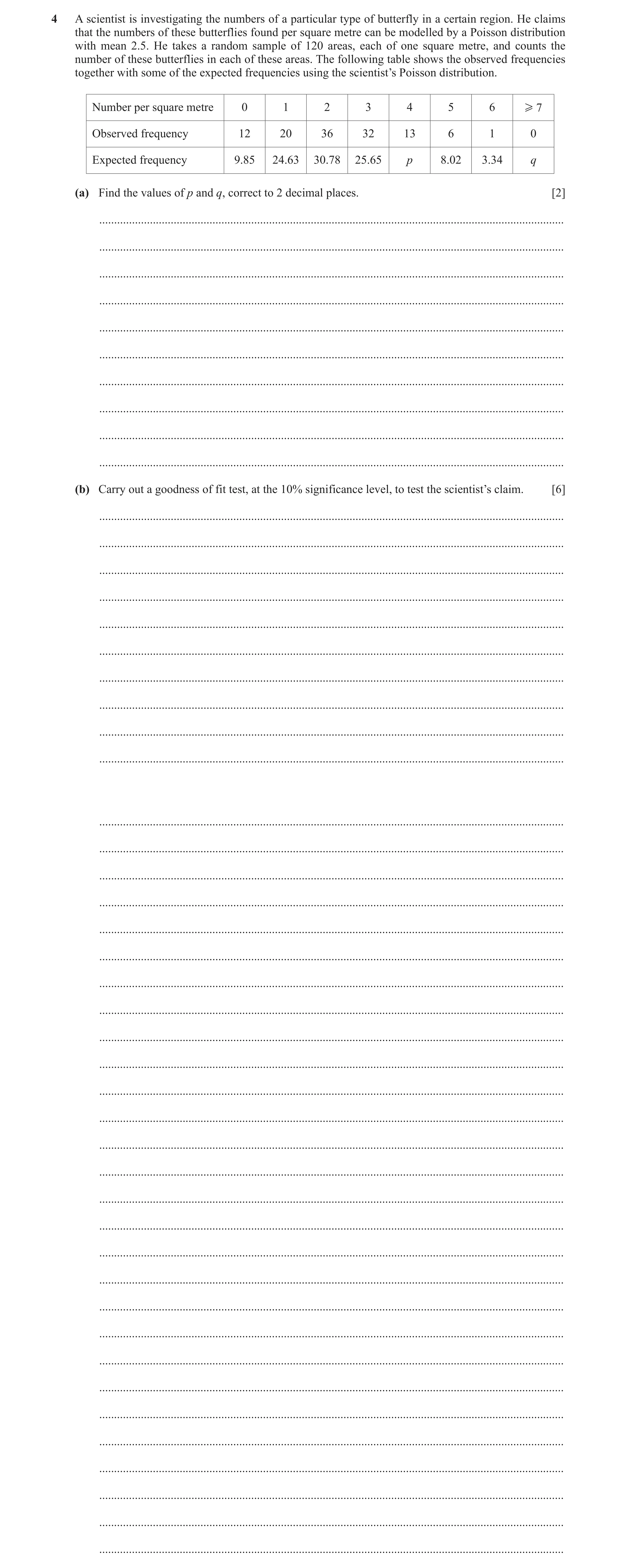
4 A scientist is investigating the numbers of a particular type of butterfly in a certain region. He claims that the numbers of these butterflies found per square metre can be modelled by a Poisson distribution with mean 2.5. He takes a random sample of 120 areas, each of one square metre, and counts the number of these butterflies in each of these areas. The following table shows the observed frequencies together with some of the expected frequencies using the scientist’s Poisson distribution. Number per square metre 0 1 2 3 4 5 6 H 7 Observed frequency 12 20 36 32 13 6 1 0 Expected frequency 9.85 24.63 30.78 25.65 p 8.02 3.34 q (a) Find the values of p and q, correct to 2 decimal places. [2] … … … … … … … … … … (b) Carry out a goodness of fit test, at the 10% significance level, to test the scientist’s claim. [6] … … … … … … … … … … … … … … … … … … … … … … … … … … … … … … … … … … … … … …
8 marks
Mark scheme: 4(a) 1.70 q B1 Condone 1.7 2 Question Answer Marks Guidance 4(b) 0 1 2 3 4 5 6 7 12 20 36 32 13 6 1 0 9.85 24.63 30.78 25.65 16.03 8.02 3.34 1.70 Combine last two columns: O value = 1, E value = 5.04 M1 Add last 2 columns (or 3 columns: 13.06). Calculate values of 2 O E E : 0.4693 0.8704 0.8853 1.5720 0.5727 0.5088 3.2384 M1 Calculate values. Test statistic = 8.12 A1 H0: data fits a Poisson distribution with mean 2.5 H1: data does not fit a Poisson distribution with mean 2.5 B1 Need data and distribution. e.g Data fits the given distribution. Number of butterflies per square metre fits Po(2.5). Critical value of chi-squared = 10.64 Compare: ‘8.12’ < 10.64, accept H0 M1 Compare their test statistic with 10.64. Note: allow 9.236 if 3 columns combined or 12.02 if none combined. There is sufficient evidence to support the scientist’s claim / there is sufficient evidence to suggest that the data fits a Poisson distribution with mean 2.5 A1 Correct conclusion, in context. Level of uncertainty in language is used. 6
This question in 9231/42 May/June 2022
Q15 · A scientist is investigating the size of shells at various beach locations 9231/43 May/June 2022
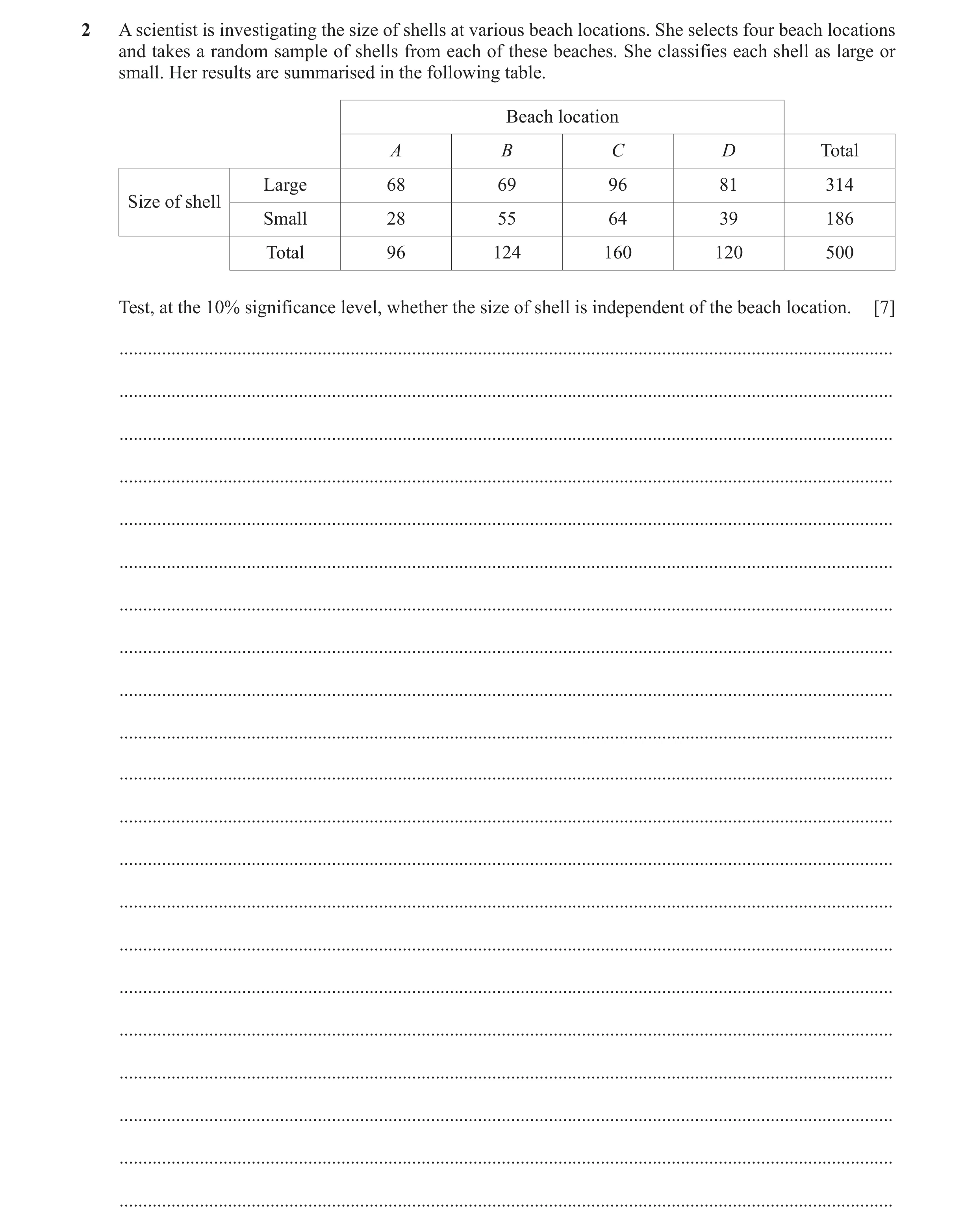
2 A scientist is investigating the size of shells at various beach locations. She selects four beach locations and takes a random sample of shells from each of these beaches. She classifies each shell as large or small. Her results are summarised in the following table. Beach location A B C D Total Large 68 69 96 81 314 Size of shell Small 28 55 64 39 186 Total 96 124 160 120 500 Test, at the 10% significance level, whether the size of shell is independent of the beach location. [7] … … … … … … … … … … … … … … … … … … … … …
7 marks
Mark scheme: 2 H0 : the size of shell is independent of the location H1 : the size of shell is not independent of the location B1 O 68 69 96 81 E 60.29 77.87 100.48 75.36 O 28 55 64 39 E 35.71 46.13 59.52 44.64 M1 A1 Attempt at calculation of E values. Calculate values of 2 O E E : 0.9859 1.0104 0.1997 0.4221 1.6646 1.7055 0.3372 0.7126 M1 Attempt at Chi-squared contributions. Accuracy of 0.1 . Test statistic = 7.04 A1 Correct total to 3sf. Tabular value for 3df = 6.251 7.04 > 6.251 Reject Ho M1 Compare with 6.251 and correct FT conclusion. May be implied by FT correct conclusion in words. Insufficient evidence to suggest size of shell is independent of location/Evidence suggests that size of shell is dependent on (beach) location A1 Correct conclusion, in context. Level of uncertainty in language is used. 7
This question in 9231/43 May/June 2022
Q16 · An organisation runs courses to train students to become engineers 9231/41 Oct/Nov 2022
2 An organisation runs courses to train students to become engineers. These students are taught in groups of 8. The director of the organisation claims that on average 60% of the students in a group achieve a pass. A random sample of 150 groups of 8 students is chosen. The following table shows the observed frequencies together with some of the expected frequencies using the appropriate binomial distribution. Number of passes per 0 1 2 3 4 5 6 7 8 group Observed 0 0 8 24 45 36 26 10 1 frequency Expected p 1.180 6.193 18.579 34.836 q r 13.437 2.519 frequency (a) Find the values of p, q and r giving your answers correct to 3 decimal places. [2] … … … … … … … … … (b) Carry out a goodness of fit test, at the 10% significance level, to test whether there is evidence to reject the director’s claim. [6] … … … … … … … … … … … … … … … … … … … … … … … … … … … … … … … … … … … … …
8 marks
Mark scheme: 2(a) Using B(8, 0.6) B1 One correct. p = 0.098, q = 41.804, r = 31.353 B1 Other two correct. If B0B0 scored, SCB1 if all 3 correct but not rounded to 3dp. 2 2(b) H0: the data fits the binomial distribution B(8, 0.6) B1 H1: the data does not fit the binomial distribution B(8, 0.6) Add first 3 columns: O value 8, E value 7.471 M1 AND last two columns: O value 11, E value 15.956 Both. Chi-squared sum: M1 0.0374 + 1.5817 + 2.9655 + 0.8058 + 0.9139 + 1.5394 Method must be seen. 7.84 A1 If M0 awarded SCB1 for 7.84. Critical value, 5df = 9.236 M1 Compare calculated value with 9.236 OR 7.84 < 9.236 13.36 if no columns added. Accept H0 12.02 adding only last 2 columns. 10.64 adding only first 3 columns. There is insufficient evidence to reject the director’s claim. A1 Correct work only except possibly B1 for hypotheses, in context, level of uncertainty in language. ‘prove’ scores A0 6
This question in 9231/41 Oct/Nov 2022
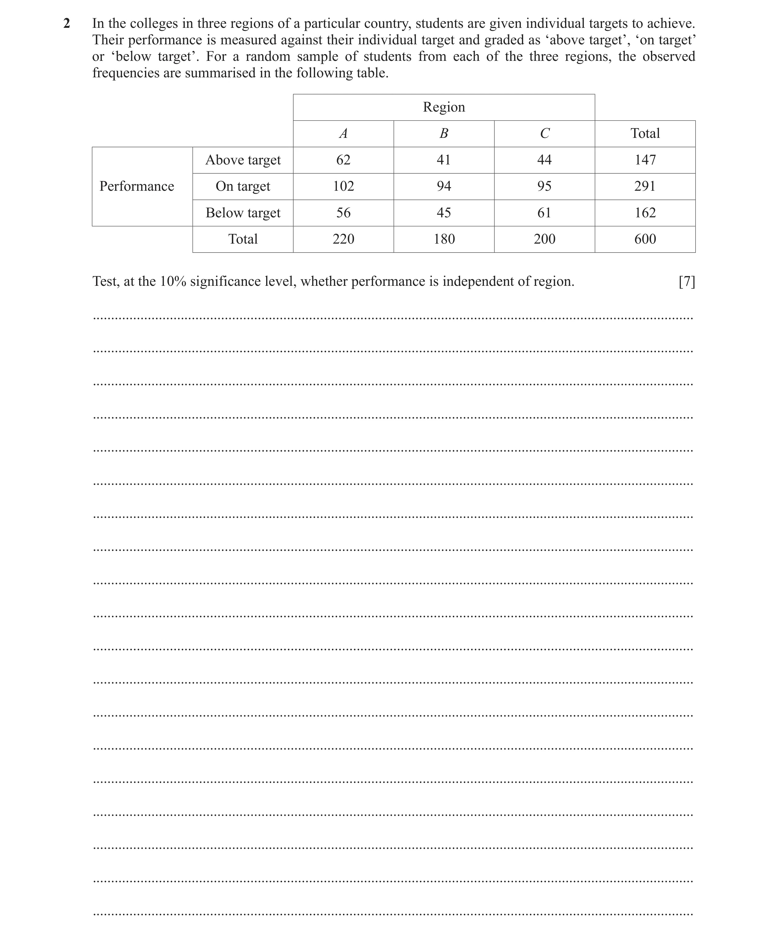
Q17 · In the colleges in three regions of a particular country, students are given individual… 9231/42 Oct/Nov 2022
2 In the colleges in three regions of a particular country, students are given individual targets to achieve. Their performance is measured against their individual target and graded as ‘above target’, ‘on target’ or ‘below target’. For a random sample of students from each of the three regions, the observed frequencies are summarised in the following table. Region A B C Total Above target 62 41 44 147 Performance On target 102 94 95 291 Below target 56 45 61 162 Total 220 180 200 600 Test, at the 10% significance level, whether performance is independent of region. [7] … … … … … … … … … … … … … … … … … … …
7 marks
Mark scheme: 2 H0: performance is independent of region B1 H1: performance is not independent of region M1 A1 Calculate expected frequencies, allow 1 error. 62 (53.9) 41 (44.1) 44 (49) 102 (106.7) 94 (87.3) 95 (97) 56 (59.4) 45 (48.6) 61 (54) Test stat = 1.217 + 0.218 + 0.510 + 0.207 + 0.514 + 0.041 + 0.195 M1 Calculate test statistic. + 0.267 + 0.907 4.08 A1 SCB2 for 4.08 if totally unsupported. SCM1A1 B1 for 4.08 supported only by expected frequencies. Tabular value, 4df = 7.779 M1 Compare with 7.779 and conclusion. 1.08 < 7.779 Accept H0 Insufficient evidence that performance is not independent of A1 Correct conclusion in context, following correct work, level of region uncertainty in language. ‘Prove’ gives A0. 7
This question in 9231/42 Oct/Nov 2022
Q18 · An organisation runs courses to train students to become engineers 9231/43 Oct/Nov 2022
2 An organisation runs courses to train students to become engineers. These students are taught in groups of 8. The director of the organisation claims that on average 60% of the students in a group achieve a pass. A random sample of 150 groups of 8 students is chosen. The following table shows the observed frequencies together with some of the expected frequencies using the appropriate binomial distribution. Number of passes per 0 1 2 3 4 5 6 7 8 group Observed 0 0 8 24 45 36 26 10 1 frequency Expected p 1.180 6.193 18.579 34.836 q r 13.437 2.519 frequency (a) Find the values of p, q and r giving your answers correct to 3 decimal places. [2] … … … … … … … … … (b) Carry out a goodness of fit test, at the 10% significance level, to test whether there is evidence to reject the director’s claim. [6] … … … … … … … … … … … … … … … … … … … … … … … … … … … … … … … … … … … … …
8 marks
Mark scheme: 2(a) Using B(8, 0.6) B1 One correct. p = 0.098, q = 41.804, r = 31.353 B1 Other two correct. If B0B0 scored, SCB1 if all 3 correct but not rounded to 3dp. 2 2(b) H0: the data fits the binomial distribution B(8, 0.6) B1 H1: the data does not fit the binomial distribution B(8, 0.6) Add first 3 columns: O value 8, E value 7.471 M1 AND last two columns: O value 11, E value 15.956 Both. Chi-squared sum: M1 0.0374 + 1.5817 + 2.9655 + 0.8058 + 0.9139 + 1.5394 Method must be seen. 7.84 A1 If M0 awarded SCB1 for 7.84. Critical value, 5df = 9.236 M1 Compare calculated value with 9.236 OR 7.84 < 9.236 13.36 if no columns added. Accept H0 12.02 adding only last 2 columns. 10.64 adding only first 3 columns. There is insufficient evidence to reject the director’s claim. A1 Correct work only except possibly B1 for hypotheses, in context, level of uncertainty in language. ‘prove’ scores A0 6
This question in 9231/43 Oct/Nov 2022
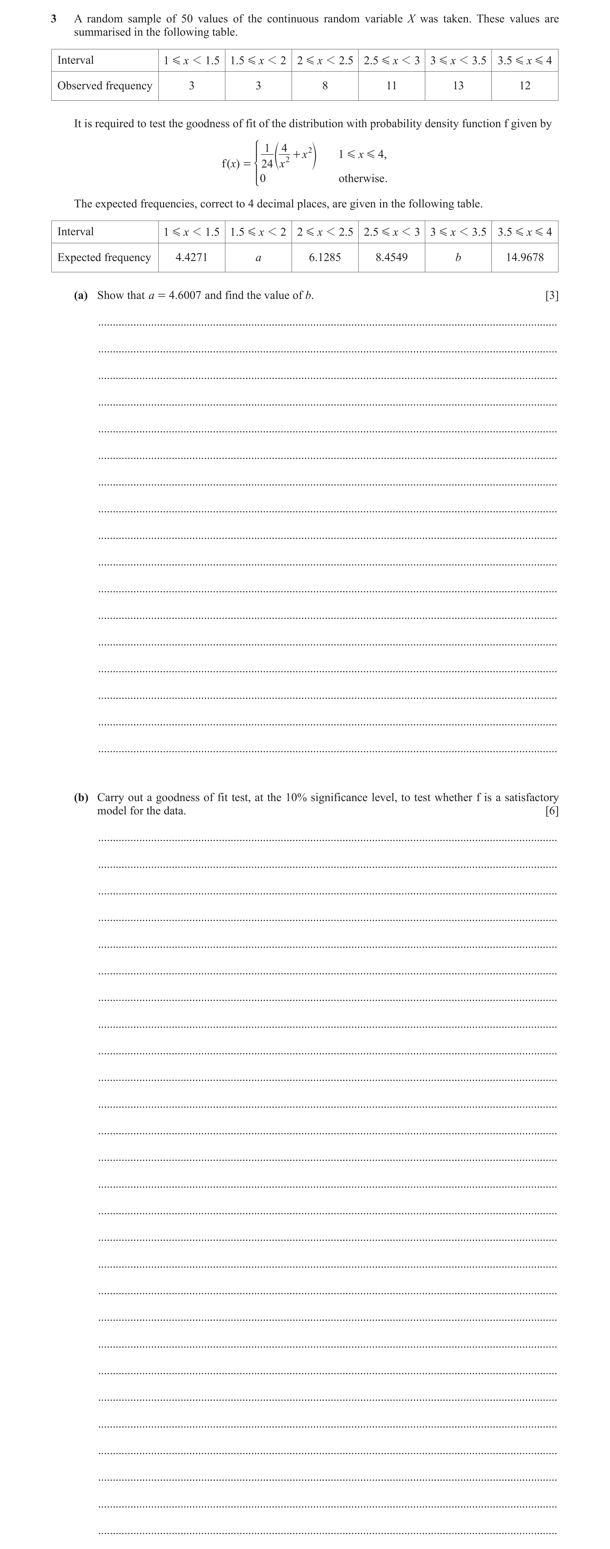
Q19 · A random sample of 50 values of the continuous random variable X was taken 9231/41 May/June 2023
3 A random sample of 50 values of the continuous random variable X was taken. These values are summarised in the following table. Interval 1 G x 1 1 .5 1.5 G x 1 2 2 G x 1 2.5 2.5 G x 1 3 3 G x 1 3.5 3.5 G x G 4 Observed frequency 3 3 8 11 13 12 It is required to test the goodness of fit of the distribution with probability density function f given by 1 4 2 + x 1 G x G 4, 2 f ( x) = * 024e x o otherwise . The expected frequencies, correct to 4 decimal places, are given in the following table. Interval 1 G x 1 1.5 1.5 G x 1 2 2 G x 1 2.5 2.5 G x 1 3 3 G x 1 3.5 3.5 G x G 4 Expected frequency 4.4271 a 6.1285 8.4549 b 14.9678 (a) Show that a = 4.6007 and find the value of b. [3] … … … … … … … … … … … … … … … … … (b) Carry out a goodness of fit test, at the 10% significance level, to test whether f is a satisfactory model for the data. [6] … … … … … … … … … … … … … … … … … … … … … … … … … … …
9 marks
Mark scheme: 3(a) 3 2 2 2 1.5 1 4 1 4 d 24 24 3 x x x x x M1 Integration with correct powers and correct limits seen. 50 a 0.092014 = 4.6007 A1 AG 53 576 or 1325 288 or 0.092014 or 4.60069 seen 11.4211 b B1 Or 11.421(0) 3 3(b) Combine first two columns: 6, 9.0278 M1 Must be seen, or implied by 1.0155. Calculate value of chi-squared: 1.0155 + 0.5715 + 0.7661 + 0.2183 + 0.5885 M1 At least 2 correct values (at least 3sf) or expressions seen. Allow columns not combined or three columns combined. 3.16 A1 CWO. Dependent on M1M1 scored. SCB1 for 3.16 with no working H0: f is a good fit for the data H1: f is not a good fit for the data B1 Tabular value of chi-squared: 7.78 ‘3.16’ < 7.78 and accept H0 M1 Correct tabular value: allow correct FT value if columns not combined (9.236) or three columns combined (6.251). Insufficient evidence to suggest that f is not a good fit for the data Condone: sufficient evidence to suggest that f is a good fit for the data. A1 Correct conclusion in context, following correct work, level of uncertainty in language (not ‘prove’, not ‘there is no evidence’), no contradictions. A0 if hypotheses reversed 6
This question in 9231/41 May/June 2023
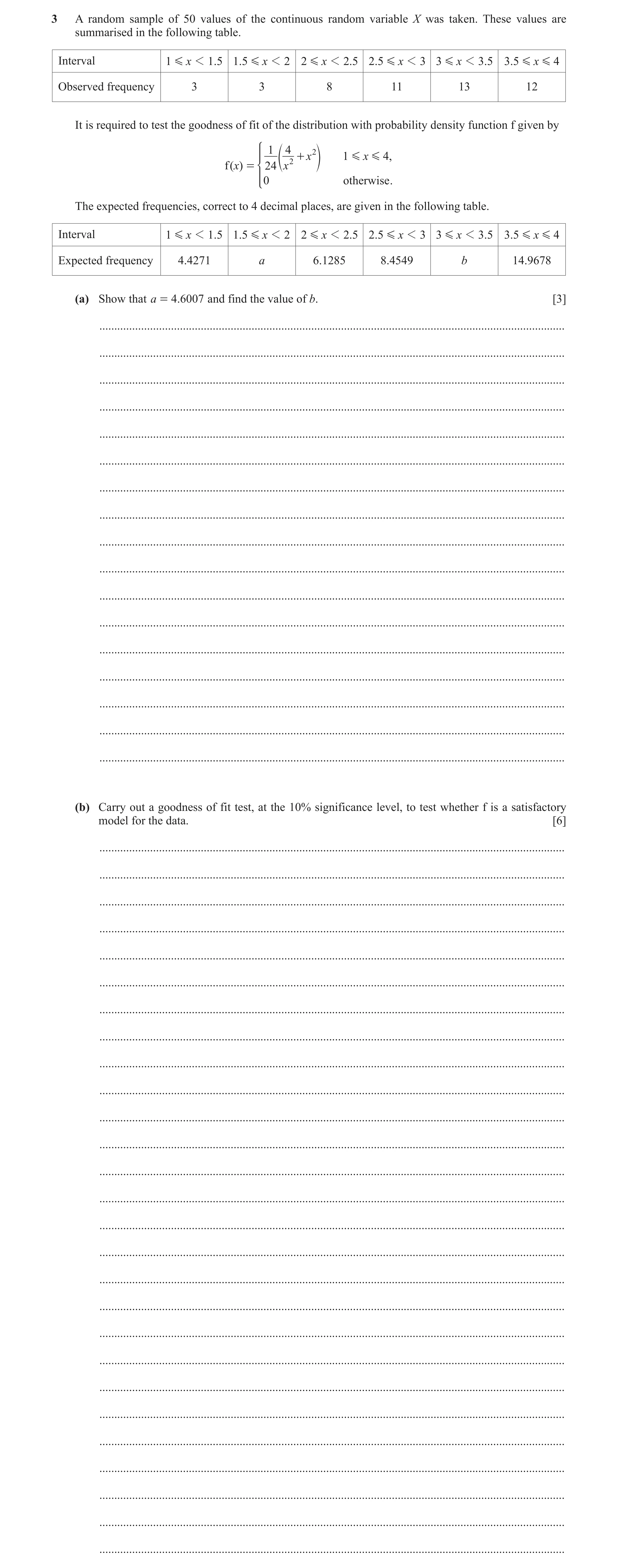
Q20 · A random sample of 50 values of the continuous random variable X was taken 9231/42 May/June 2023
3 A random sample of 50 values of the continuous random variable X was taken. These values are summarised in the following table. Interval 1 G x 1 1 .5 1.5 G x 1 2 2 G x 1 2.5 2.5 G x 1 3 3 G x 1 3.5 3.5 G x G 4 Observed frequency 3 3 8 11 13 12 It is required to test the goodness of fit of the distribution with probability density function f given by 1 4 2 + x 1 G x G 4, 2 f ( x) = * 024e x o otherwise . The expected frequencies, correct to 4 decimal places, are given in the following table. Interval 1 G x 1 1.5 1.5 G x 1 2 2 G x 1 2.5 2.5 G x 1 3 3 G x 1 3.5 3.5 G x G 4 Expected frequency 4.4271 a 6.1285 8.4549 b 14.9678 (a) Show that a = 4.6007 and find the value of b. [3] … … … … … … … … … … … … … … … … … (b) Carry out a goodness of fit test, at the 10% significance level, to test whether f is a satisfactory model for the data. [6] … … … … … … … … … … … … … … … … … … … … … … … … … … …
9 marks
Mark scheme: 3(a) 3 2 2 2 1.5 1 4 1 4 d 24 24 3 x x x x x M1 Integration with correct powers and correct limits seen. 50 a 0.092014 = 4.6007 A1 AG 53 576 or 1325 288 or 0.092014 or 4.60069 seen 11.4211 b B1 Or 11.421(0) 3 3(b) Combine first two columns: 6, 9.0278 M1 Must be seen, or implied by 1.0155. Calculate value of chi-squared: 1.0155 + 0.5715 + 0.7661 + 0.2183 + 0.5885 M1 At least 2 correct values (at least 3sf) or expressions seen. Allow columns not combined or three columns combined. 3.16 A1 CWO. Dependent on M1M1 scored. SCB1 for 3.16 with no working H0: f is a good fit for the data H1: f is not a good fit for the data B1 Tabular value of chi-squared: 7.78 ‘3.16’ < 7.78 and accept H0 M1 Correct tabular value: allow correct FT value if columns not combined (9.236) or three columns combined (6.251). Insufficient evidence to suggest that f is not a good fit for the data Condone: sufficient evidence to suggest that f is a good fit for the data. A1 Correct conclusion in context, following correct work, level of uncertainty in language (not ‘prove’, not ‘there is no evidence’), no contradictions. A0 if hypotheses reversed 6
This question in 9231/42 May/June 2023
Q21 · A scientist is investigating whether the ability to remember depends on age 9231/43 May/June 2023
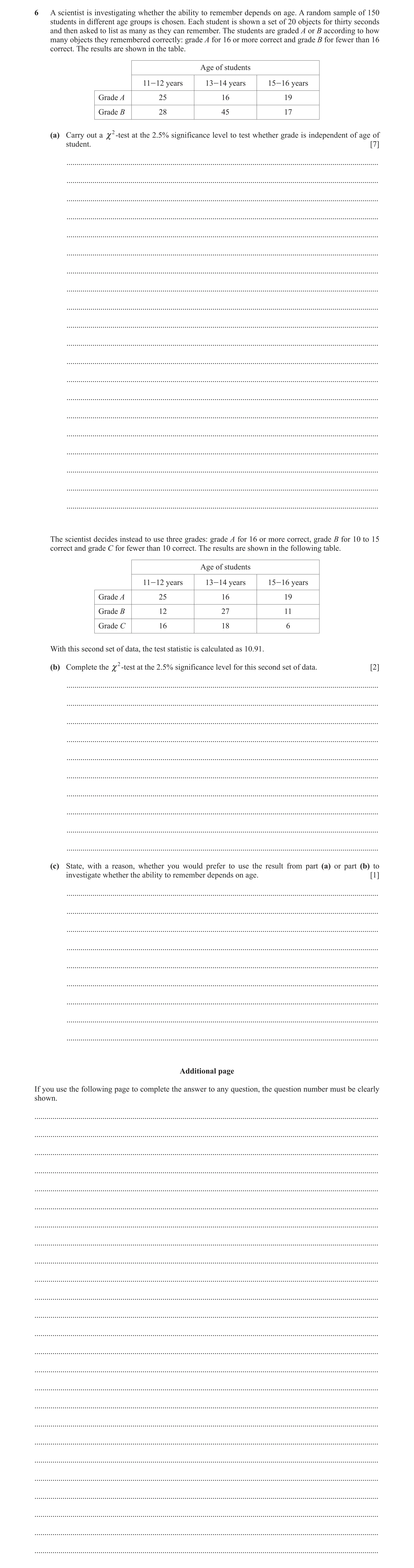
6 A scientist is investigating whether the ability to remember depends on age. A random sample of 150 students in different age groups is chosen. Each student is shown a set of 20 objects for thirty seconds and then asked to list as many as they can remember. The students are graded A or B according to how many objects they remembered correctly: grade A for 16 or more correct and grade B for fewer than 16 correct. The results are shown in the table. Age of students 11-12 years 13-14 years 15-16 years Grade A 25 16 19 Grade B 28 45 17 (a) Carry out a | 2 -test at the 2.5% significance level to test whether grade is independent of age of student. [7] … … … … … … … … … … … … … … … … … … … … The scientist decides instead to use three grades: grade A for 16 or more correct, grade B for 10 to 15 correct and grade C for fewer than 10 correct. The results are shown in the following table. Age of students 11-12 years 13-14 years 15-16 years Grade A 25 16 19 Grade B 12 27 11 Grade C 16 18 6 With this second set of data, the test statistic is calculated as 10.91. (b) Complete the | 2 -test at the 2.5% significance level for this second set of data. [2] … … … … … … … … … … (c) State, with a reason, whether you would prefer to use the result from part (a) or part (b) to investigate whether the ability to remember depends on age. [1] … … … … … … … … … Additional page If you use the following page to complete the answer to any question, the question number must be clearly shown. … … … … … … … … … … … … … … … … … … … … … … … … …
10 marks
Mark scheme: 6(a) H0: grade is independent of age H1: grade is not independent of age B1 Condone ‘Ability to remember’ instead of ‘grade’. Calculate expected values, shown in table in bold 25 21.2 16 24.4 19 14.4 60 28 31.8 45 36.6 17 21.6 90 53 61 36 150 M1 At least 2 correct values or expressions. A1 6 correct values or expressions. Calculate chi-squared values: 0.6811 + 2.8918 + 1.4694 + 0.4541 + 1.9279 + 0.9796 M1 At least 2 correct values (at least 3sf) or expressions seen. 8.40[4] A1 Tabular value, 2 degrees of freedom = 7.378 ‘8.404’ > 7.378 and reject H0/significant M1 Compare their value with 7.378 and conclusion without context. Condone ‘accept H1’. Sufficient evidence to suggest that grade is not independent of age. A1 Correct conclusion in context, following correct work, level of uncertainty in language (not ‘prove’, not ‘there is no evidence’), no contradictions. A0 if hypotheses wrong way round. 7 6(b) Value, 4 degrees of freedom = 11.14 10.91 < 11.14 Accept H0/not significant M1 Condone ‘reject H1’. Insufficient evidence to suggest that grade is not independent of age. A1 CAO 2 Question Answer Marks Guidance 6(c) For example, result in part (b) because the table contains more information e.g. More degrees of freedom, more groups, more detail B1 Any appropriate comment to support part (a) or part (b). Allow ‘more specific’. Not ‘more data’ or ‘more accurate’ on its own. 1
This question in 9231/43 May/June 2023
Q22 · A town council has published its plans for redeveloping the town centre and residents are… 9231/41 Oct/Nov 2023
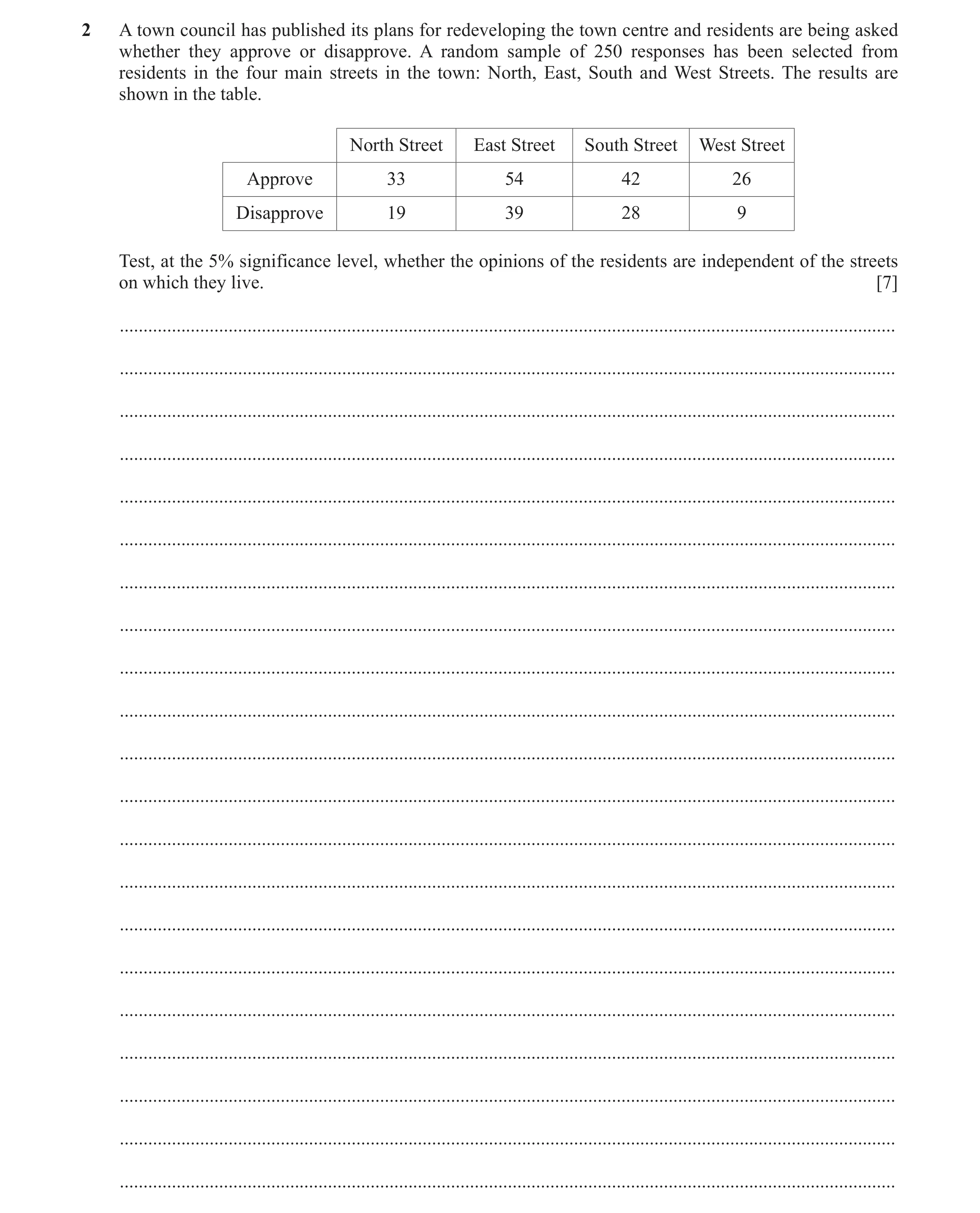
2 A town council has published its plans for redeveloping the town centre and residents are being asked whether they approve or disapprove. A random sample of 250 responses has been selected from residents in the four main streets in the town: North, East, South and West Streets. The results are shown in the table. North Street East Street South Street West Street Approve 33 54 42 26 Disapprove 19 39 28 9 Test, at the 5% significance level, whether the opinions of the residents are independent of the streets on which they live. [7] … … … … … … … … … … … … … … … … … … … … …
7 marks
Mark scheme: 2 H0: opinion is independent of street H1: opinion is not independent of street B1 M1 At least 2 correct values or expressions. 33 32.24 54 57.66 42 43.4 26 21.7 155 A1 6 correct values or expressions. 19 19.76 39 35.34 28 26.6 9 13.3 95 52 93 70 35 250 Calculate chi-squared values: M1 Correct to 3 decimal places. 0.0179 + 0.2323 + 0.0452 + 0.8521 + 0.0292 + 0.3790 + 0.0737 + 1.3902 At least 2 correct values or expressions. 3.02 A1 SC B1 3.02 following M1M0 SC B2 3.02 following M0M0 Tabular value, 3 degrees of freedom 7.815: ‘3.02’ < 7.815, accept H0 M1 Allow ‘not significant’. Insufficient evidence to suggest that opinion depends on street. A1 CWO. Correct conclusion in context, following correct work, level of uncertainty in language. A0 if hypotheses wrong way round or missing. 7
This question in 9231/41 Oct/Nov 2023
Q23 · The number of breakdowns on a particular section of road is recorded each day over a… 9231/42 Oct/Nov 2023
2 The number of breakdowns on a particular section of road is recorded each day over a period of 90 days. It is suggested that the number of breakdowns follows a Poisson distribution with mean 3.5. The data is summarised in the table, together with some of the expected frequencies resulting from the suggested Poisson distribution. Number of 8 or 0 1 2 3 4 5 6 7 breakdowns per day more Observed frequency 0 5 13 17 21 16 9 5 4 Expected frequency 2.718 9.512 16.646 16.993 11.895 3.469 2.407 (a) Complete the table. [2] … … … … … … … … (b) Carry out a goodness of fit test, at the 10% significance level, to determine whether or not Po(3.5) is a good fit to the data. [6] … … … … … … … … … … … … … … … … … … … … … … … … … … … … … … … … … … … … … … …
8 marks
Mark scheme: 2(a) B1 Each. 0 5 13 17 21 16 9 5 4 B1 2.718 9.512 16.646 19.421 16.993 11.895 6.939 3.469 2.407 2 2(b) H0: Po(3.5) is a good fit to the data B1 H1: Po(3.5) is not a good fit to the data Combine first 2 columns: 5, 12.23 M1 Both. And last 2 columns: 9, 5.876 Chi-squared values: M1 Allow if no or incorrect number of columns 4.274 + 0.799 + 0.302 + 0.945 + 1.417 + 0.612 + 1.661 added. At least two ‘correct’ values (3 sf) or expressions seen from their grouping (or lack of). 2.718 + 2.140 + … + 0.6757 + 1.054 10.0 A1 AWRT 10.0 If M0 awarded then SC B1 for 10.0. Tabular value: 10.64 ‘10.0’ < 10.64, accept H0 /not significant M1 Allow equivalent to 10.64 if columns not combined or only one pair combined (12.02 one pair combined, 13.36 none combined). Insufficient evidence to suggest that Po(3.5) is not a good fit to the data A1 Correct conclusion in context, following correct work, level of uncertainty in language. A0 if hypotheses the wrong way round or missing. 6
This question in 9231/42 Oct/Nov 2023
Q24 · A town council has published its plans for redeveloping the town centre and residents are… 9231/43 Oct/Nov 2023
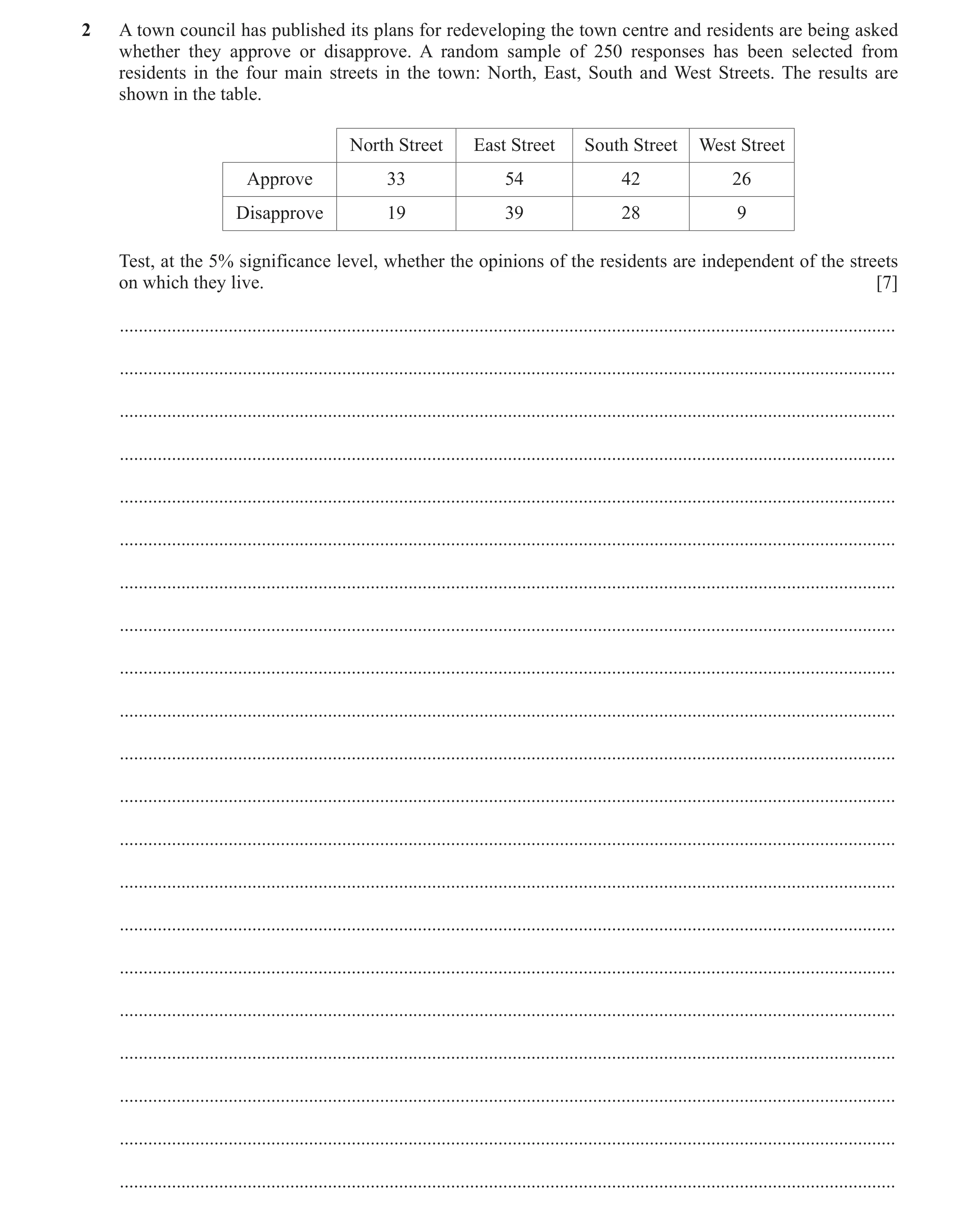
2 A town council has published its plans for redeveloping the town centre and residents are being asked whether they approve or disapprove. A random sample of 250 responses has been selected from residents in the four main streets in the town: North, East, South and West Streets. The results are shown in the table. North Street East Street South Street West Street Approve 33 54 42 26 Disapprove 19 39 28 9 Test, at the 5% significance level, whether the opinions of the residents are independent of the streets on which they live. [7] … … … … … … … … … … … … … … … … … … … … …
7 marks
Mark scheme: 2 H0: opinion is independent of street H1: opinion is not independent of street B1 M1 At least 2 correct values or expressions. 33 32.24 54 57.66 42 43.4 26 21.7 155 A1 6 correct values or expressions. 19 19.76 39 35.34 28 26.6 9 13.3 95 52 93 70 35 250 Calculate chi-squared values: M1 Correct to 3 decimal places. 0.0179 + 0.2323 + 0.0452 + 0.8521 + 0.0292 + 0.3790 + 0.0737 + 1.3902 At least 2 correct values or expressions. 3.02 A1 SC B1 3.02 following M1M0 SC B2 3.02 following M0M0 Tabular value, 3 degrees of freedom 7.815: ‘3.02’ < 7.815, accept H0 M1 Allow ‘not significant’. Insufficient evidence to suggest that opinion depends on street. A1 CWO. Correct conclusion in context, following correct work, level of uncertainty in language. A0 if hypotheses wrong way round or missing. 7
This question in 9231/43 Oct/Nov 2023
Q25 · Two companies, P and Q, produce a certain type of paint brush 9231/41 May/June 2024
5 Two companies, P and Q, produce a certain type of paint brush. An independent examiner rates the quality of the brushes produced as poor, satisfactory or good. He takes a random sample of brushes from each company. The examiner’s ratings are summarised in the table. Company Poor Satisfactory Good P 18 43 64 Q 22 22 31 (a) Test, at the 5% significance level, whether quality of brushes is independent of company. [7] … … … … … … … … … … … … … … … … … … … … … … … … … … … … … … … … … … … … … … … … … (b) Compare the quality of the brushes produced by the two companies. [1] … … … … … … … …
8 marks
Mark scheme: 5(a) Company Poor Satisfactory Good P (18) 25 (43) 40.625 (64) 59.375 Q (22) 15 (22) 24.375 (31) 35.625 M1 A1 Calculate E values to at least 2dp, allow one error. These must be seen. For A1, working to at least 2dp. Chi-squared contributions: Company Poor Satisfactory Good P 1.96 0.1388 0.3603 Q 3.2667 0.2314 0.6004 M1 At least 2 correct values or expressions seen. Or may be implied by AWRT 6.56 Test statistic = 6.56 A1 AWRT 6.56. H0: Quality (of items) is independent of company H1: Quality (of items) is not independent of company B1 Condone ‘no association/relationship between….’ ‘association/relationship between….’. 6.56 > 5.991 Reject H0 M1 ‘6.56’ from their attempt at chi-squared, 5.991 must be correct. Consistent signs in comparison. FT conclusion from their 6.56. Condone ‘Accept H1’. ‘Reject H0’ can be implied by a conclusion that is consistent with their 6.56. Question Answer Marks Guidance 5(a) There is sufficient evidence to suggest that the quality of brushes is not independent of company. A1 Correct work only, conclusion in context with level of uncertainty in language. Not ‘prove’. Accept ‘enough evidence’. Condone ‘some evidence’. Do not accept ‘there is insufficient…’. 7 5(b) P produces better quality brushes (than Q) or Q produces worse quality brushes (than P) P has fewer poor quality brushes than expected AND Q has more poor quality brushes than expected B1 Condone P is better (than Q). 1
This question in 9231/41 May/June 2024
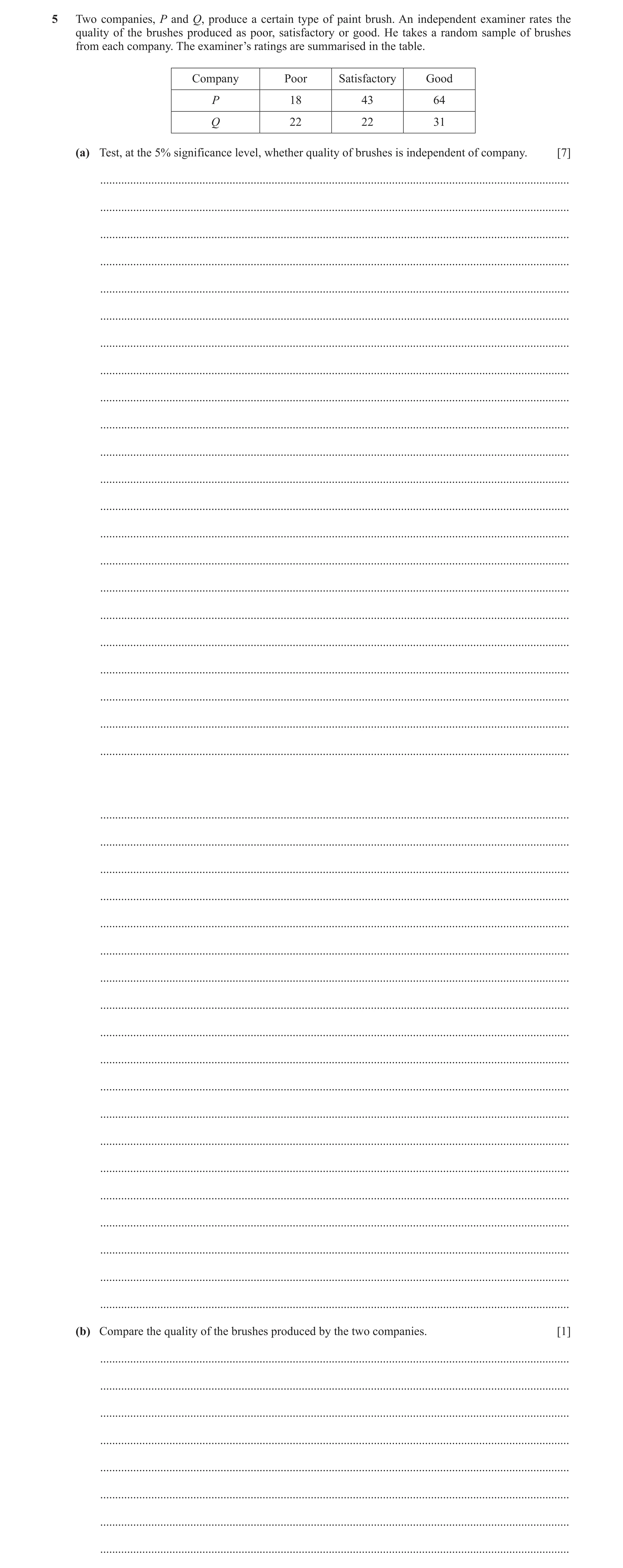
Q26 · Two companies, P and Q, produce a certain type of paint brush 9231/42 May/June 2024
5 Two companies, P and Q, produce a certain type of paint brush. An independent examiner rates the quality of the brushes produced as poor, satisfactory or good. He takes a random sample of brushes from each company. The examiner’s ratings are summarised in the table. Company Poor Satisfactory Good P 18 43 64 Q 22 22 31 (a) Test, at the 5% significance level, whether quality of brushes is independent of company. [7] … … … … … … … … … … … … … … … … … … … … … … … … … … … … … … … … … … … … … … … … … (b) Compare the quality of the brushes produced by the two companies. [1] … … … … … … … …
8 marks
Mark scheme: 5(a) Company Poor Satisfactory Good P (18) 25 (43) 40.625 (64) 59.375 Q (22) 15 (22) 24.375 (31) 35.625 M1 A1 Calculate E values to at least 2dp, allow one error. These must be seen. For A1, working to at least 2dp. Chi-squared contributions: Company Poor Satisfactory Good P 1.96 0.1388 0.3603 Q 3.2667 0.2314 0.6004 M1 At least 2 correct values or expressions seen. Or may be implied by AWRT 6.56 Test statistic = 6.56 A1 AWRT 6.56. H0: Quality (of items) is independent of company H1: Quality (of items) is not independent of company B1 Condone ‘no association/relationship between….’ ‘association/relationship between….’. 6.56 > 5.991 Reject H0 M1 ‘6.56’ from their attempt at chi-squared, 5.991 must be correct. Consistent signs in comparison. FT conclusion from their 6.56. Condone ‘Accept H1’. ‘Reject H0’ can be implied by a conclusion that is consistent with their 6.56. Question Answer Marks Guidance 5(a) There is sufficient evidence to suggest that the quality of brushes is not independent of company. A1 Correct work only, conclusion in context with level of uncertainty in language. Not ‘prove’. Accept ‘enough evidence’. Condone ‘some evidence’. Do not accept ‘there is insufficient…’. 7 5(b) P produces better quality brushes (than Q) or Q produces worse quality brushes (than P) P has fewer poor quality brushes than expected AND Q has more poor quality brushes than expected B1 Condone P is better (than Q). 1
This question in 9231/42 May/June 2024
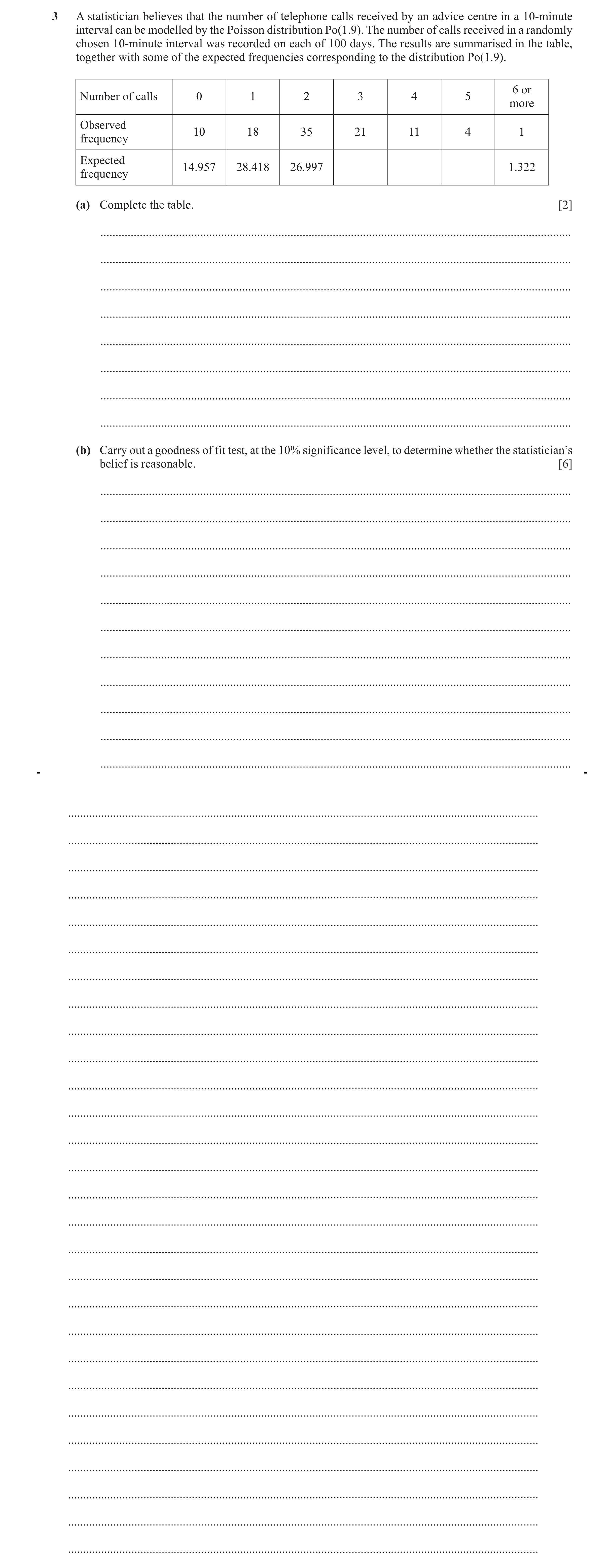
Q27 · A statistician believes that the number of telephone calls received by an advice centre… 9231/41 Oct/Nov 2024
3 A statistician believes that the number of telephone calls received by an advice centre in a 10-minute interval can be modelled by the Poisson distribution Po(1.9). The number of calls received in a randomly chosen 10-minute interval was recorded on each of 100 days. The results are summarised in the table, together with some of the expected frequencies corresponding to the distribution Po(1.9). 6 or Number of calls 0 1 2 3 4 5 more Observed 10 18 35 21 11 4 1 frequency Expected 14.957 28.418 26.997 1.322 frequency (a) Complete the table. [2] … … … … … … … … (b) Carry out a goodness of fit test, at the 10% significance level, to determine whether the statistician’s belief is reasonable. [6] … … … … … … … … … … … … … … … … … … … … … … … … … … … … … … … … … … … … … … …
8 marks
Mark scheme: 3(a) 17.098 8.122 3.086 B1 One correct. B1 All correct. 2 3(b) M1 0 1 2 3 4 or more Last two or three columns combined. 10 18 35 21 16 14.957 28.418 26.997 17.098 12.53 Contributions to test statistic are: M1 1.6428 3.8192 2.3724 0.8905 0.9609(7) May be implied by awrt 9.69 Test statistic is 9.69 A1 9.686 H0: Po(1.9) is a good fit for the data B1 H1: Po(1.9) is not a good fit for the data Critical value is 7.779, compare ‘9.69’ > 7.779 reject H0 M1 4 degrees of freedom Sufficient evidence to suggest that Po(1.9) is a not a good fit for the data/ A1 Correct work only, including hypotheses, in Sufficient evidence to reject/not support the statistician’s claim context, level of uncertainty in language. 6
This question in 9231/41 Oct/Nov 2024
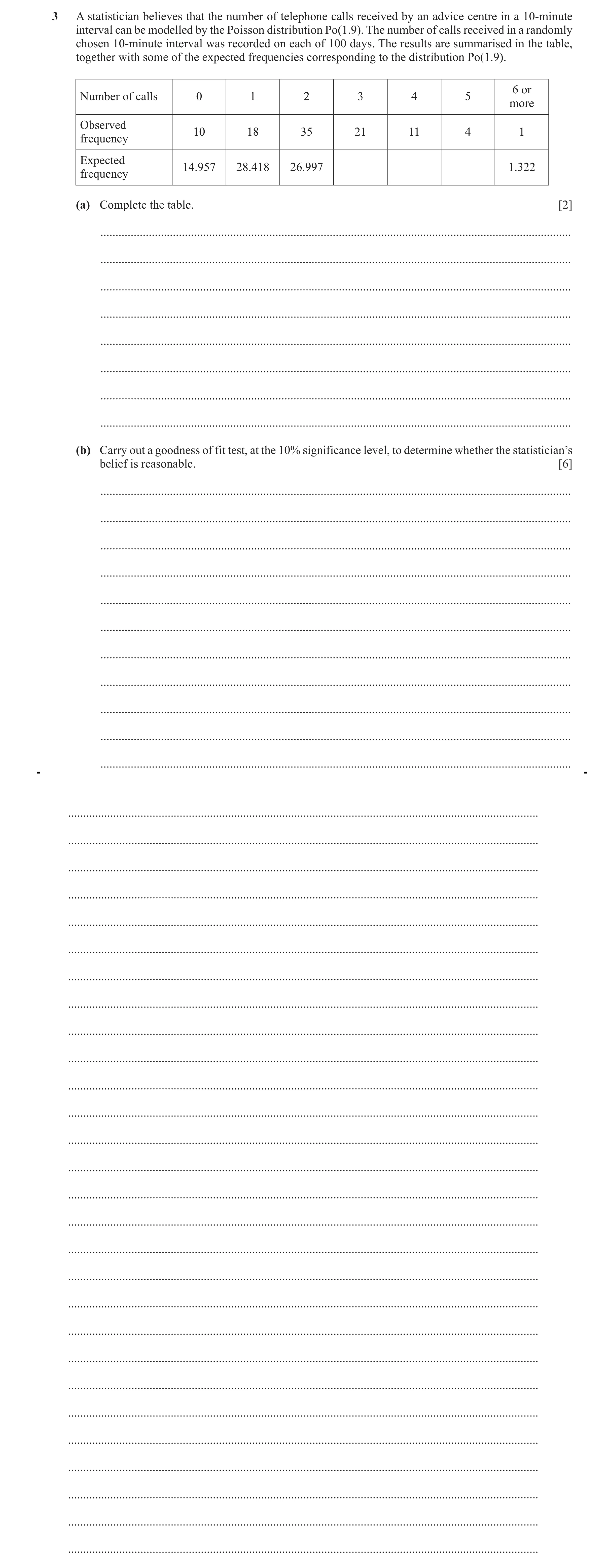
Q28 · A statistician believes that the number of telephone calls received by an advice centre… 9231/43 Oct/Nov 2024
3 A statistician believes that the number of telephone calls received by an advice centre in a 10-minute interval can be modelled by the Poisson distribution Po(1.9). The number of calls received in a randomly chosen 10-minute interval was recorded on each of 100 days. The results are summarised in the table, together with some of the expected frequencies corresponding to the distribution Po(1.9). 6 or Number of calls 0 1 2 3 4 5 more Observed 10 18 35 21 11 4 1 frequency Expected 14.957 28.418 26.997 1.322 frequency (a) Complete the table. [2] … … … … … … … … (b) Carry out a goodness of fit test, at the 10% significance level, to determine whether the statistician’s belief is reasonable. [6] … … … … … … … … … … … … … … … … … … … … … … … … … … … … … … … … … … … … … … …
8 marks
Mark scheme: 3(a) 17.098 8.122 3.086 B1 One correct. B1 All correct. 2 3(b) M1 0 1 2 3 4 or more Last two or three columns combined. 10 18 35 21 16 14.957 28.418 26.997 17.098 12.53 Contributions to test statistic are: M1 1.6428 3.8192 2.3724 0.8905 0.9609(7) May be implied by awrt 9.69 Test statistic is 9.69 A1 9.686 H0: Po(1.9) is a good fit for the data B1 H1: Po(1.9) is not a good fit for the data Critical value is 7.779, compare ‘9.69’ > 7.779 reject H0 M1 4 degrees of freedom Sufficient evidence to suggest that Po(1.9) is a not a good fit for the data/ A1 Correct work only, including hypotheses, in Sufficient evidence to reject/not support the statistician’s claim context, level of uncertainty in language. 6
This question in 9231/43 Oct/Nov 2024
Q29 · A shop selling electrical goods has a team of three salespeople: Avril, Ben and Charlie 9231/44 May/June 2025
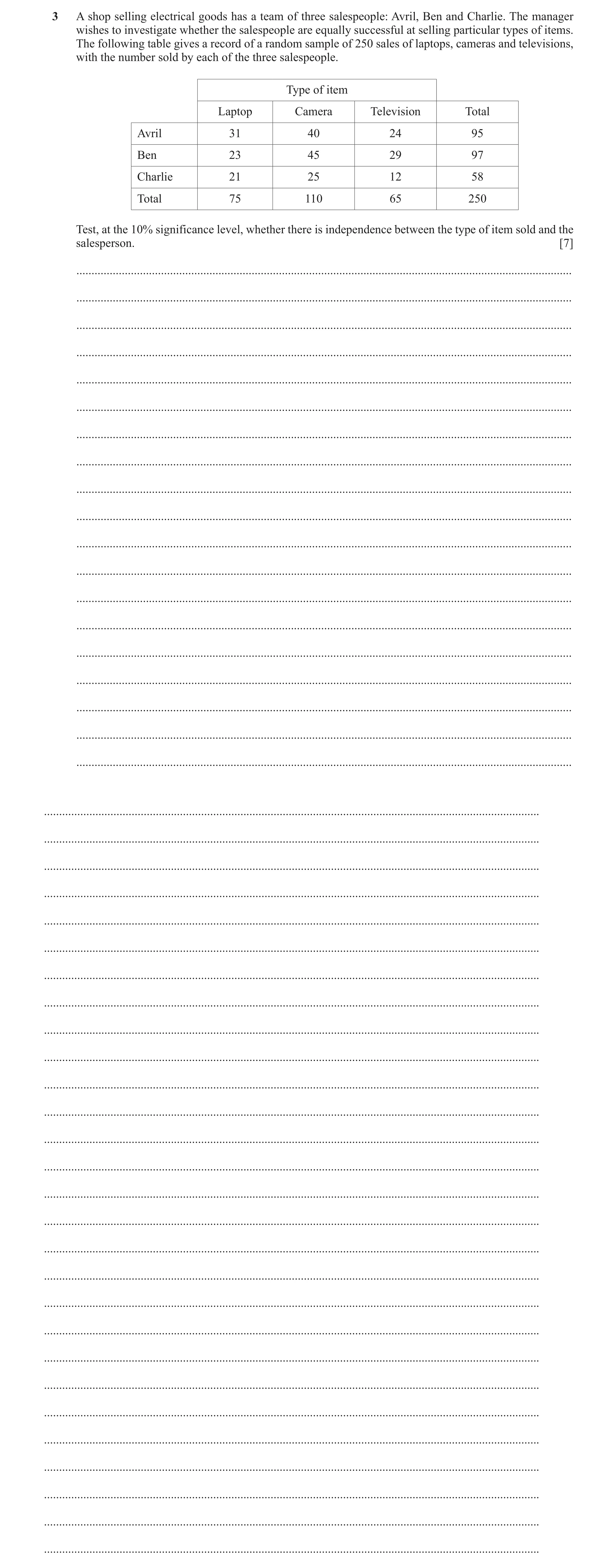
3 A shop selling electrical goods has a team of three salespeople: Avril, Ben and Charlie. The manager wishes to investigate whether the salespeople are equally successful at selling particular types of items. The following table gives a record of a random sample of 250 sales of laptops, cameras and televisions, with the number sold by each of the three salespeople. Type of item Laptop Camera Television Total Avril 31 40 24 95 Ben 23 45 29 97 Charlie 21 25 12 58 Total 75 110 65 250 Test, at the 10% significance level, whether there is independence between the type of item sold and the salesperson. [7] … … … … … … … … … … … … … … … … … … … … … … … … … … … … … … … … … … … … … … … … … … … … … … …
7 marks
Mark scheme: 3 H 0 : type of item sold is independent of salesperson. B1 Allow dependent, association or relationship for not independent. For example: H0: No association/relationship between… H1 : type of item sold is not independent of salesperson. H1: Association/relationship between… Laptop Camera Television M1 Calculate expected values (must be seen). M1 for at least 4 expected values correct to 3sf or better. Avril 31 (28.5) 40 (41.80) 24 (24.70) Ben 23 (29.1) 45 (42.68) 29 (25.22) A1 All expected values correct to 3sf or better. Charlie 21 (17.4) 25 (25.52) 12 (15.08) ( 31 − 28.5 ) 2 ( 40 − 41.8 ) 2 (15.08 − 12 ) 2 M1 At least 2 terms (not including 250) of correct form seen. + ++ May see individual terms not summed. 28.5 41.8 15.08 May be implied by AWRT 3.67 or 3.68. OR 312 40 2 12 2 + ++ − 250 28.5 41.8 15.08 Test statistic = 3.67 (or 3.68) A1 AWRT 3.67 or 3.68. '3.67' < 7.779, accept H 0 (not significant). M1 Compare their 3.67 (or 3.68) with 7.779 and appropriate conclusion (may be in terms of H1). Accept H0 can be implied by an attempt at an appropriate conclusion in context. Allow M1 for comparison of their 3.67 (or 3.68) with 9.488 and appropriate conclusion. Insufficient evidence to suggest that type of item sold and A1 Correct conclusion in context from correct working ignoring salesperson are not independent. hypotheses. Condone ‘no sufficient evidence’. OR Level of uncertainty in language used (for example, not ‘prove’). Insufficient evidence to suggest that there is dependence between Must refer to both item and salesperson. type of item sold and salesperson. Do not accept statements such as ‘there is sufficient evidence to suggest…’. 7
This question in 9231/44 May/June 2025
Q30 · The manager of a car park claims that the number of cars entering the car park follows a… 9231/41 Oct/Nov 2025
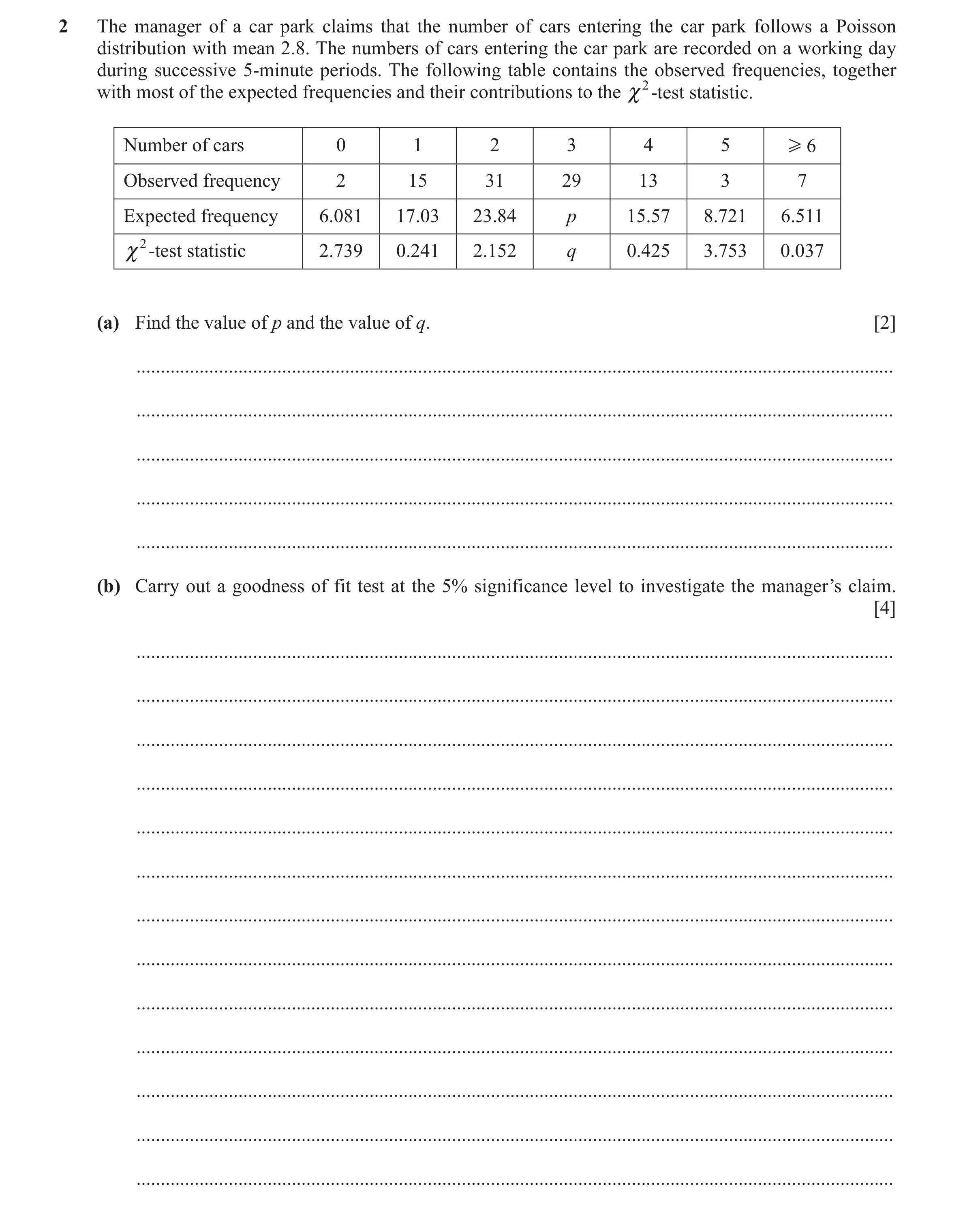
2 The manager of a car park claims that the number of cars entering the car park follows a Poisson distribution with mean 2.8. The numbers of cars entering the car park are recorded on a working day during successive 5-minute periods. The following table contains the observed frequencies, together with most of the expected frequencies and their contributions to the | 2 -test statistic. Number of cars 0 1 2 3 4 5 H 6 Observed frequency 2 15 31 29 13 3 7 Expected frequency 6.081 17.03 23.84 p 15.57 8.721 6.511 | 2 -test statistic 2.739 0.241 2.152 q 0.425 3.753 0.037 (a) Find the value of p and the value of q. [2] … … … … … (b) Carry out a goodness of fit test at the 5% significance level to investigate the manager’s claim. [4] … … … … … … … … … … … … …
6 marks
Mark scheme: 2(a) e −2.8 (2.8) 3 B1 Or by subtraction. p = 100 = 22.248 Allow 22.2 or 22.3. 3! (29 − 22.25) 2 B1 AWRT 2.05. q = = 2.05 22.25 2 2(b) H0: Po(2.8) fits the data. B1 Must mention distribution and data/number of cars. H1: Po(2.8) does not fit the data. OR H0: Po(2.8) is a satisfactory model for the number of cars (entering the car park). H1: Po(2.8) is not a satisfactory model for the number of cars (entering the car park). 2.739 + 0.241 + 2.152 + '2.049'+ 0.425 + 3.753 + 0.037 = 11.396 M1 Sum of chi-square contributions using their q. May be implied by 11.4. '11.4' 12.59, accept H0 / do not reject H0 / not significant. M1 Compare their 11.4 with 12.59 and appropriate result (may be in terms of H1). Test result may be implied by an attempt at an appropriate conclusion in context ignoring hypotheses. Insufficient evidence to suggest that Po(2.8) is not a good fit to the A1 Correct conclusion from correct working ignoring hypotheses. data. In context. OR Level of uncertainty in language is used (for example, not ‘prove’). Insufficient evidence to suggest that the manager’s claim is false. Allow ‘Not enough evidence that / to show / conclude that…’ Do not accept statements such as ‘there is sufficient evidence to suggest…’ or ‘no evidence…..’ 4
This question in 9231/41 Oct/Nov 2025
Q31 · A traffic expert claims that the number of breakdowns occurring each day on a busy… 9231/42 Oct/Nov 2025
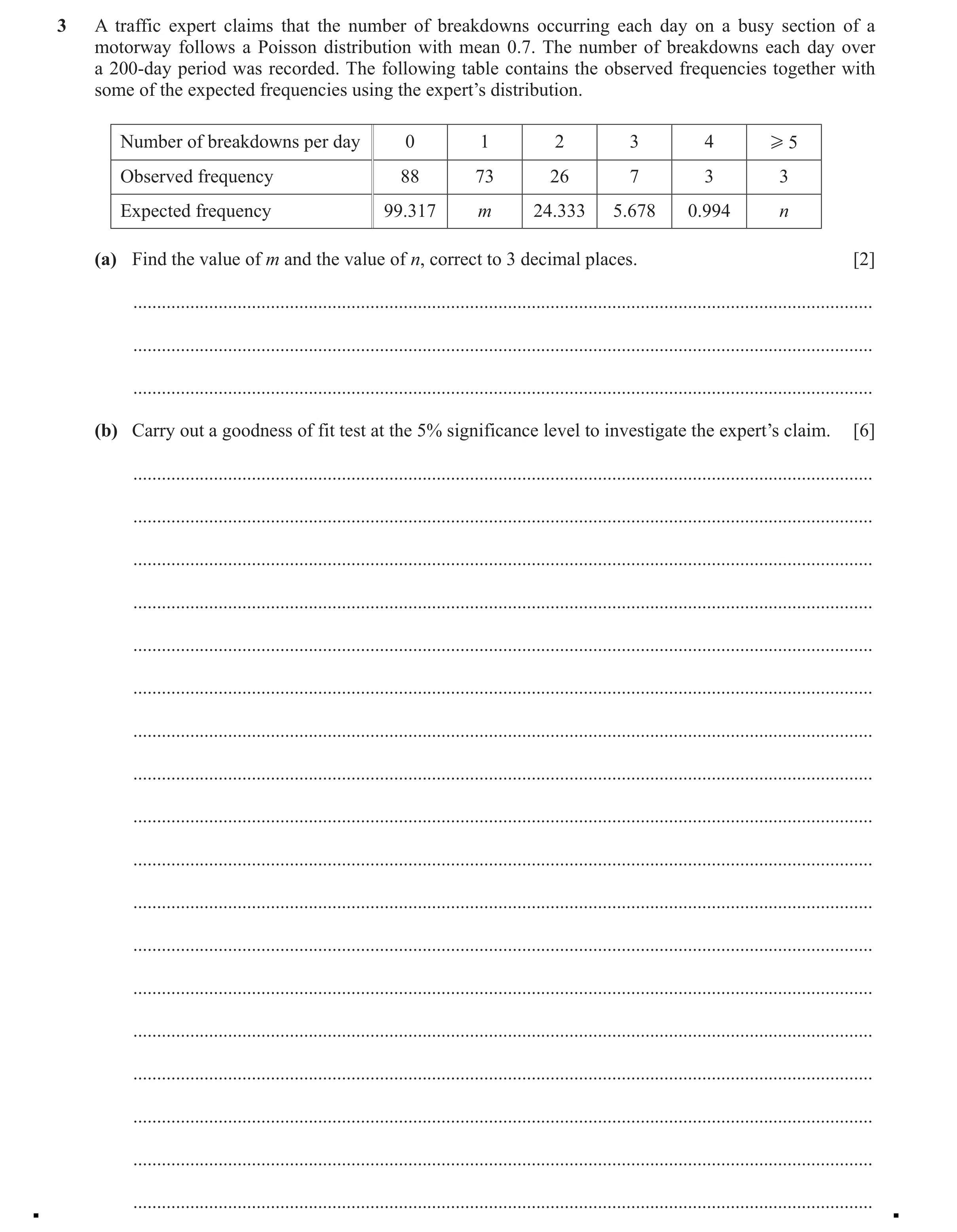
3 A traffic expert claims that the number of breakdowns occurring each day on a busy section of a motorway follows a Poisson distribution with mean 0.7. The number of breakdowns each day over a 200-day period was recorded. The following table contains the observed frequencies together with some of the expected frequencies using the expert’s distribution. Number of breakdowns per day 0 1 2 3 4 H 5 Observed frequency 88 73 26 7 3 3 Expected frequency 99.317 m 24.333 5.678 0.994 n (a) Find the value of m and the value of n, correct to 3 decimal places. [2] … … … (b) Carry out a goodness of fit test at the 5% significance level to investigate the expert’s claim. [6] … … … … … … … … … … … … … … … … … …
8 marks
Mark scheme: 3(a) m = 69.522 B1 n = 0.156 or 0.157 B1 Subtraction gives 0.156. 2 3(b) H0: Po ( 0.7 ) fits the data. B1 Must mention distribution and data/number of breakdowns. May see H0: Po ( 0.7 ) is a satisfactory model for the data. H1: Po ( 0.7 ) does not fit the data. H1: Po ( 0.7 ) is not a satisfactory model for the data. Combining last 3 columns give 13 and 6.828 or 6.829. M1 Combine expected frequencies less than 5. ( 88 − 99.317 ) 2 ( 73 − 69.552 ) 2 (13 − 6.829 ) 2 M1 At least 2 expressions (not including 200) of correct form seen. + ++ May see individual terms not summed. 99.317 69.552 6.829 May be implied by 2 contributions correct to 3sf seen. [1.2896 + 0.1740 + 0.1142 + 5.5764] 6.828 gives 5.5790. OR 882 732 26 2 132 + + + − 200 99.317 69.552 24.333 6.829 7.15 or 7.16 A1 SC B1 for 7.15 or 7.16 following M0. '7.15' 7.815 , accept H0 / do not reject H0 / not significant. M1 Compare their 7.15 with 7.815 (9.488 if 2 columns combined, 11.07 if no columns combined) and appropriate result (may be in terms of H1). Test result may be implied by an attempt at an appropriate conclusion in context ignoring hypotheses. Insufficient evidence to reject expert’s claim. A1 Correct conclusion from correct working ignoring hypotheses. OR In context. Insufficient evidence to suggest that Po ( 0.7 ) is not a good Level of uncertainty in language is used (for example, not ‘prove’) Allow ‘Not enough evidence that / to show / conclude that…’. fit/model [for the data]. Do not accept statements such as ‘there is sufficient evidence to suggest…’ or ‘no evidence…’. 6
This question in 9231/42 Oct/Nov 2025
Q32 · The manager of a car park claims that the number of cars entering the car park follows a… 9231/43 Oct/Nov 2025
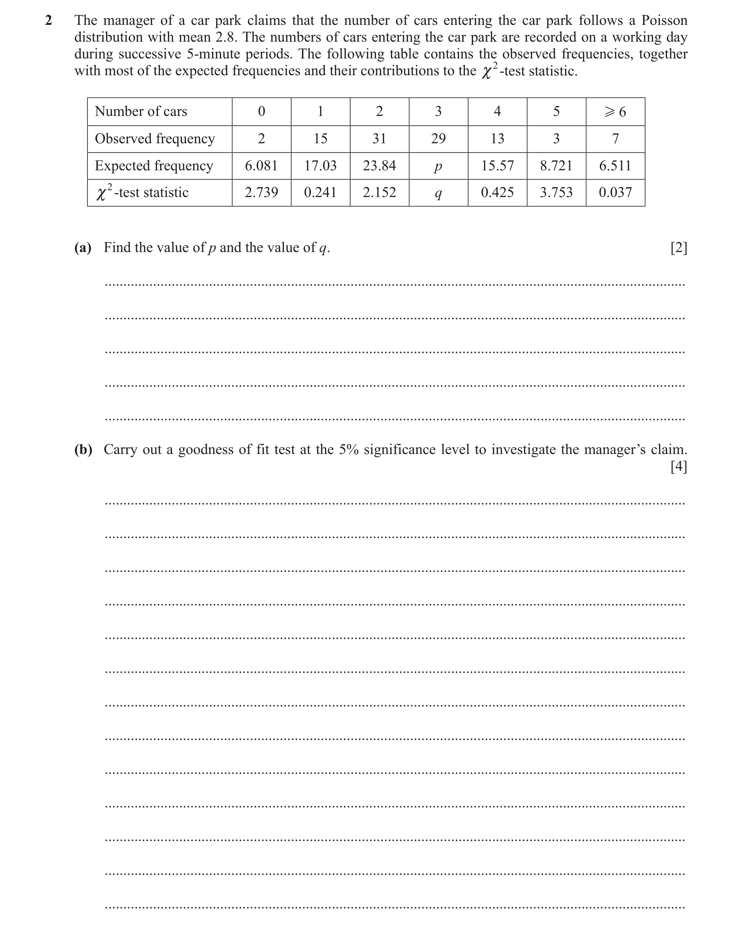
2 The manager of a car park claims that the number of cars entering the car park follows a Poisson distribution with mean 2.8. The numbers of cars entering the car park are recorded on a working day during successive 5-minute periods. The following table contains the observed frequencies, together with most of the expected frequencies and their contributions to the | 2 -test statistic. Number of cars 0 1 2 3 4 5 H 6 Observed frequency 2 15 31 29 13 3 7 Expected frequency 6.081 17.03 23.84 p 15.57 8.721 6.511 | 2 -test statistic 2.739 0.241 2.152 q 0.425 3.753 0.037 (a) Find the value of p and the value of q. [2] … … … … … (b) Carry out a goodness of fit test at the 5% significance level to investigate the manager’s claim. [4] … … … … … … … … … … … … …
6 marks
Mark scheme: 2(a) e −2.8 (2.8) 3 B1 Or by subtraction. p = 100 = 22.248 Allow 22.2 or 22.3. 3! (29 − 22.25) 2 B1 AWRT 2.05. q = = 2.05 22.25 2 2(b) H0: Po(2.8) fits the data. B1 Must mention distribution and data/number of cars. H1: Po(2.8) does not fit the data. OR H0: Po(2.8) is a satisfactory model for the number of cars (entering the car park). H1: Po(2.8) is not a satisfactory model for the number of cars (entering the car park). 2.739 + 0.241 + 2.152 + '2.049'+ 0.425 + 3.753 + 0.037 = 11.396 M1 Sum of chi-square contributions using their q. May be implied by 11.4. '11.4' 12.59, accept H0 / do not reject H0 / not significant. M1 Compare their 11.4 with 12.59 and appropriate result (may be in terms of H1). Test result may be implied by an attempt at an appropriate conclusion in context. Insufficient evidence to suggest that Po(2.8) is not a good fit to the A1 Correct conclusion from correct working ignoring hypotheses. data. In context. OR Level of uncertainty in language is used (for example, not ‘prove’). Insufficient evidence to suggest that the manager’s claim is false. Allow ‘Not enough evidence that / to show / conclude that…’ Do not accept statements such as ‘there is sufficient evidence to suggest…’ or ‘no evidence…..’ 4
This question in 9231/43 Oct/Nov 2025
 1 / 54
 2 / 54
 3 / 54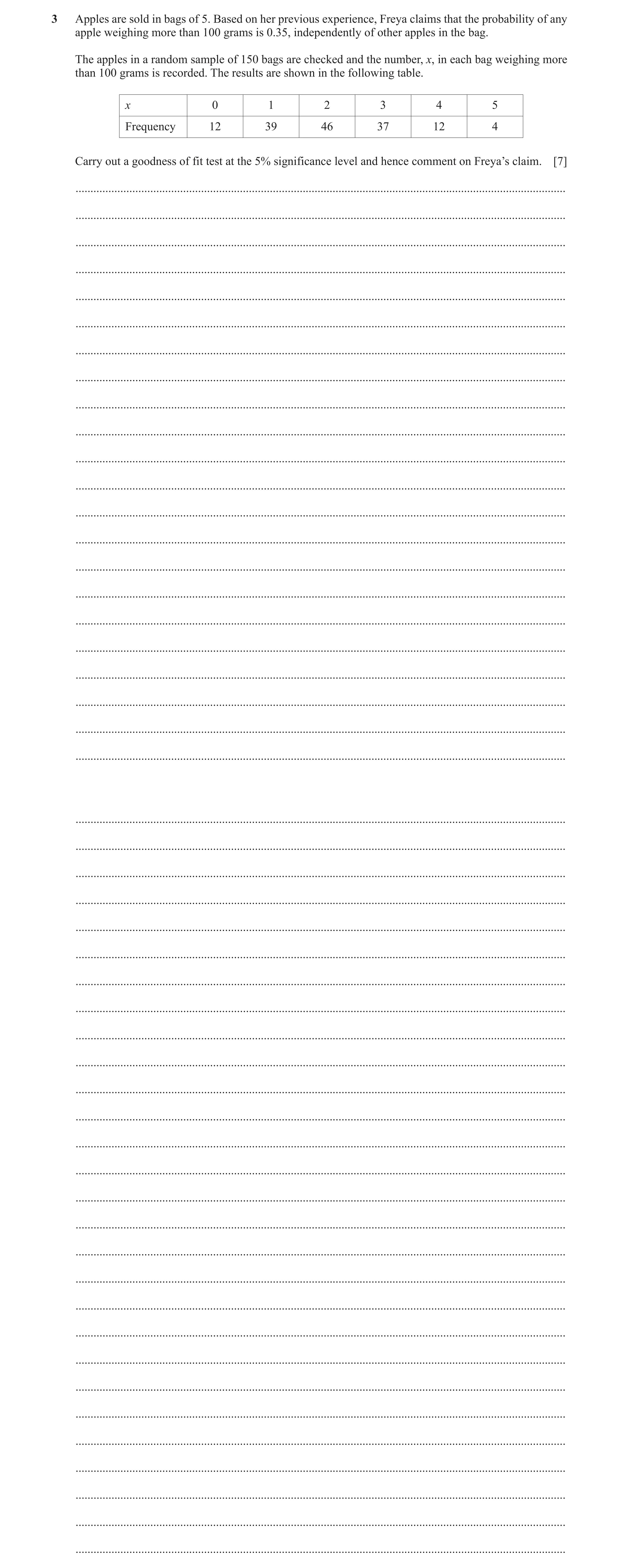
 25 / 54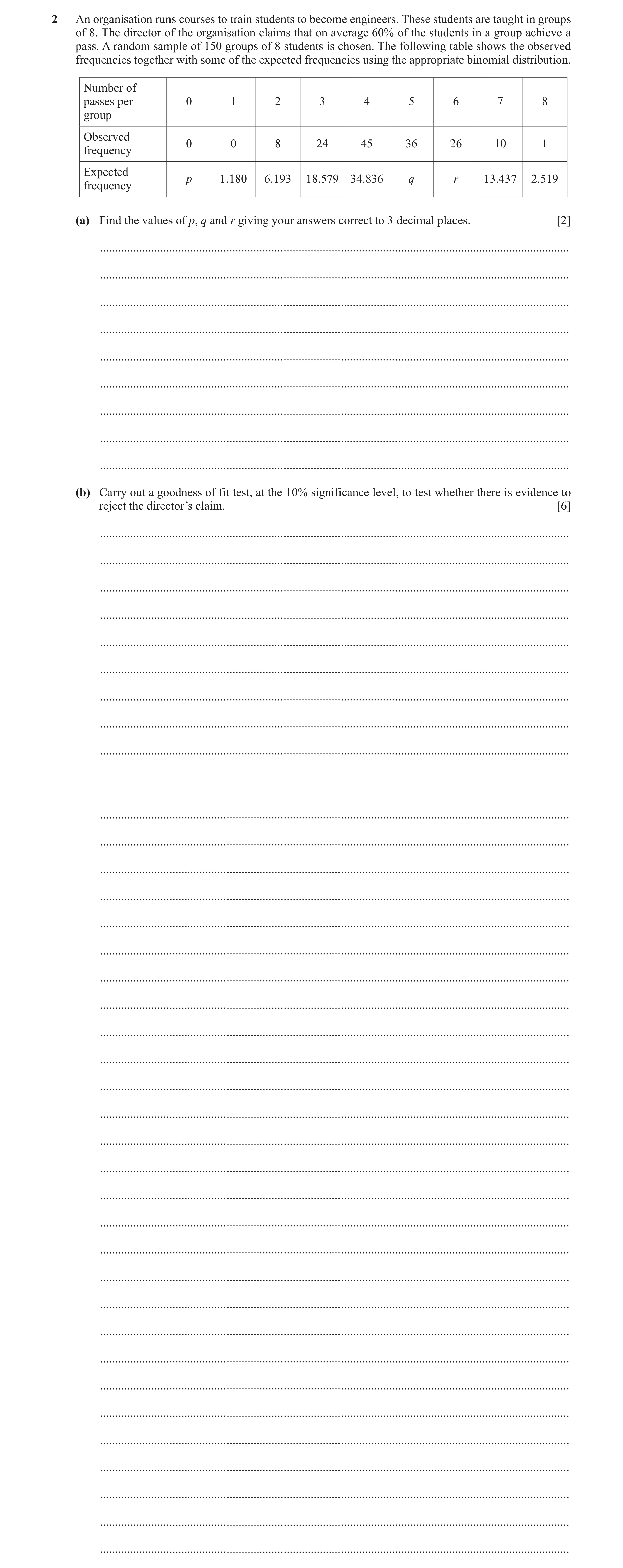
 28 / 54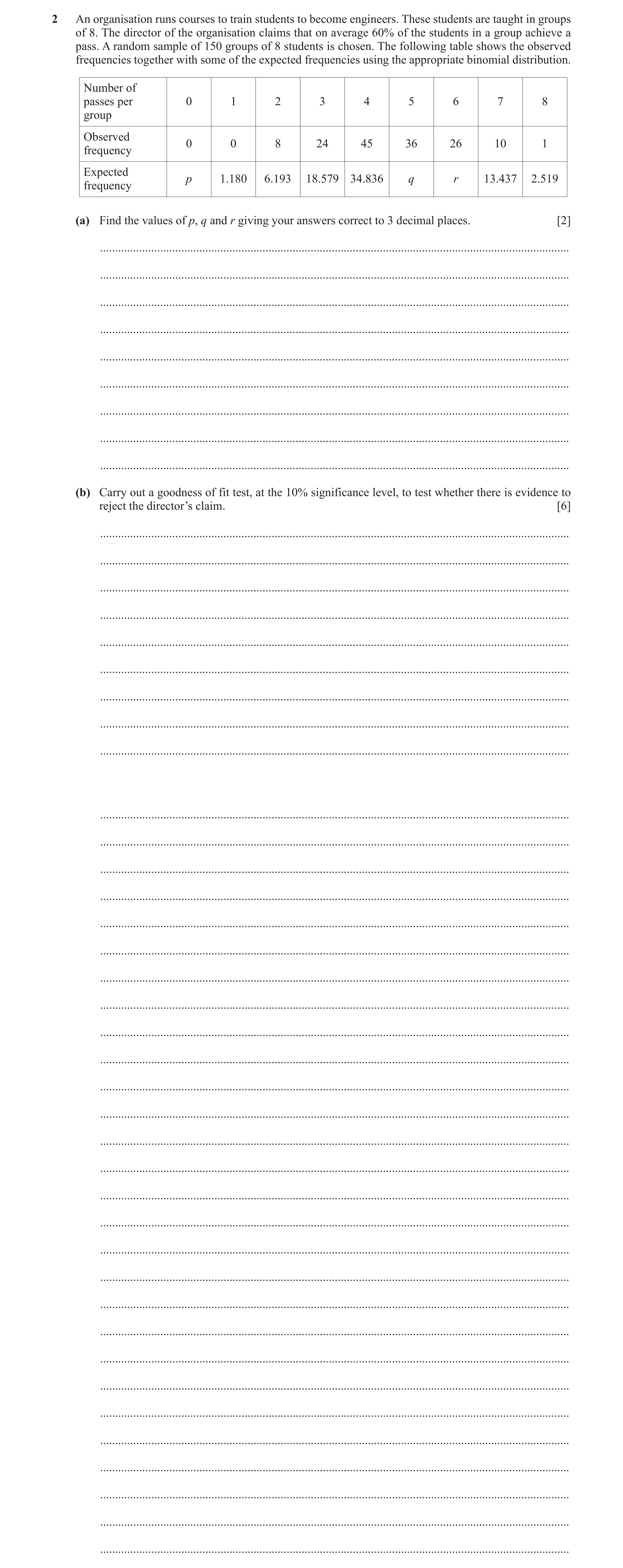
 38 / 54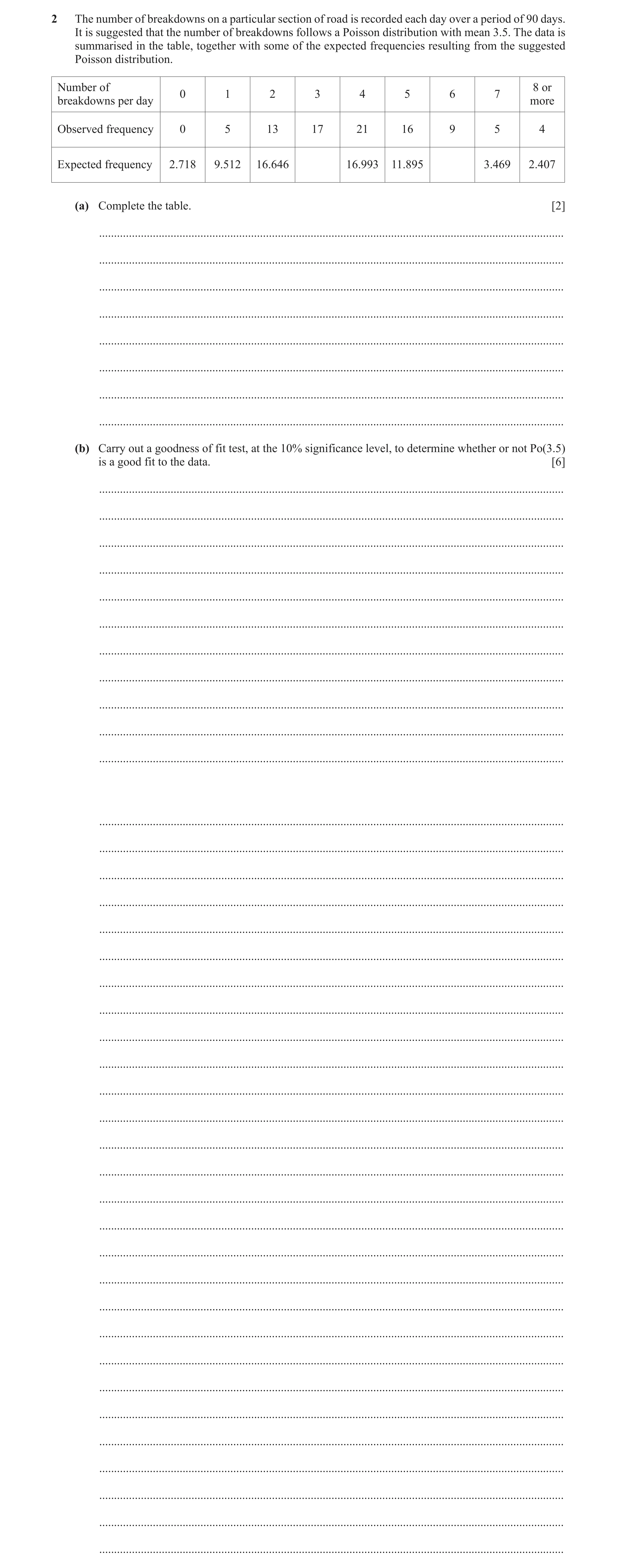
 41 / 54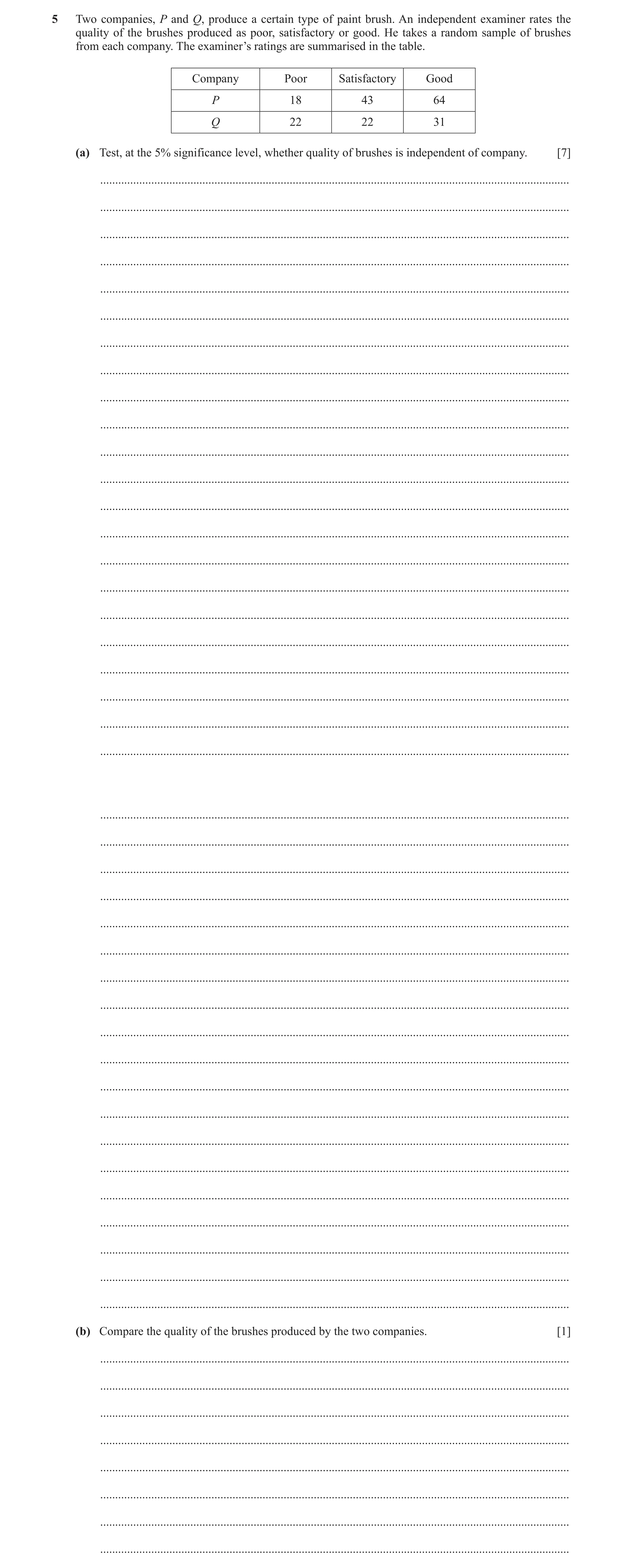
 52 / 54
 53 / 54
 54 / 54
 6
6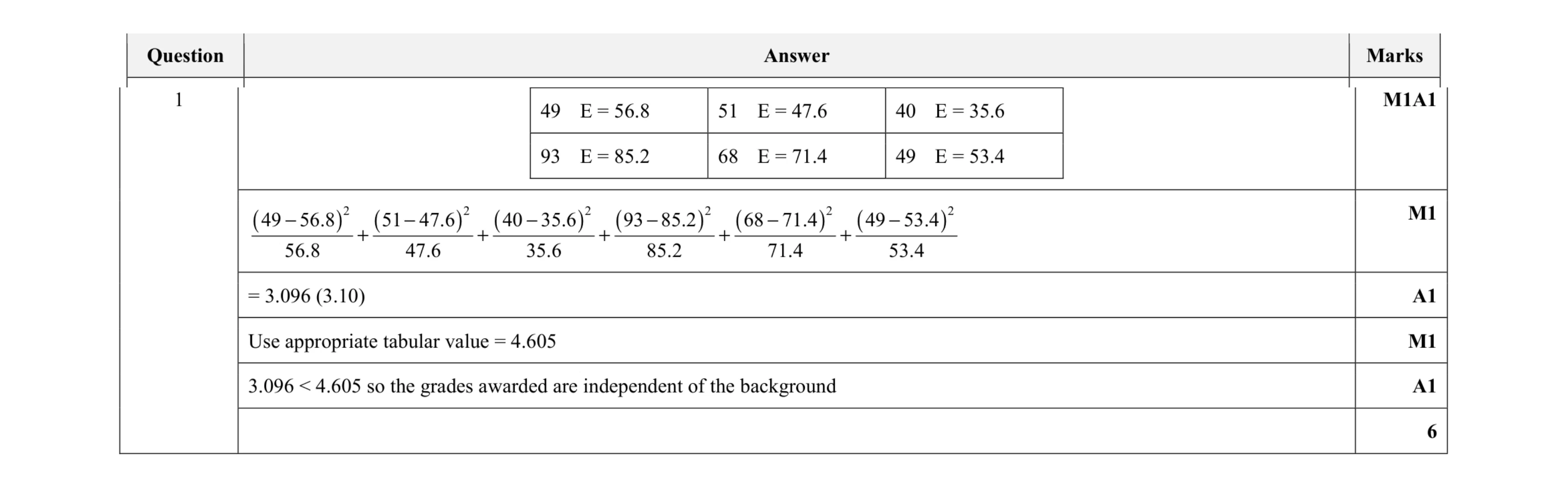 6
6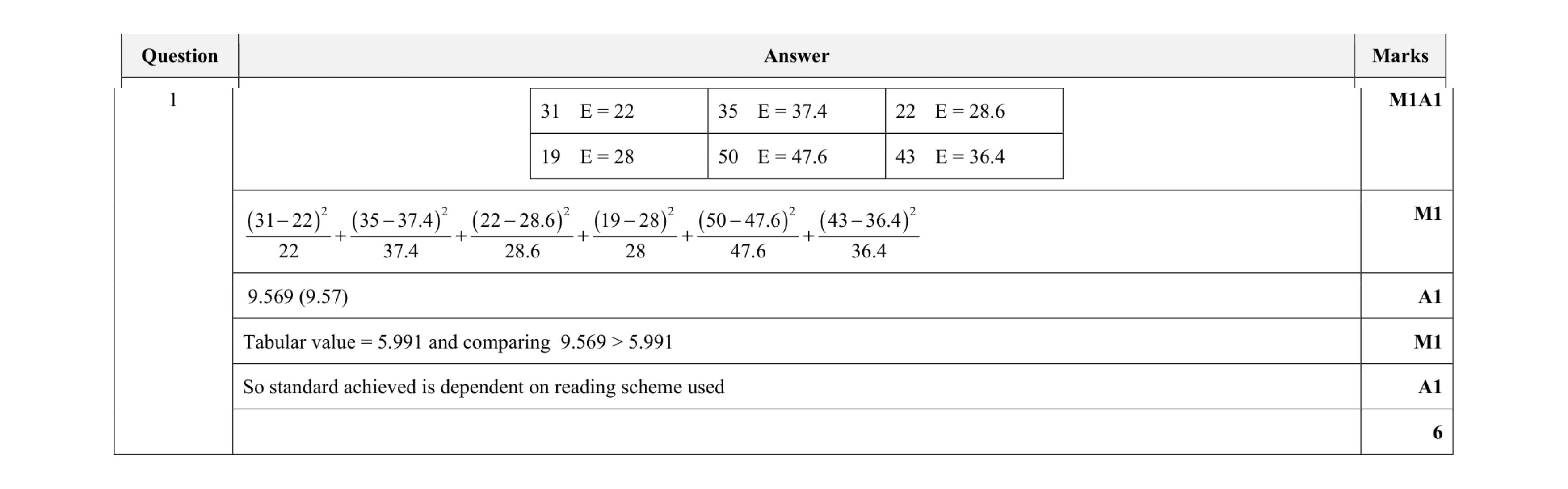 6
6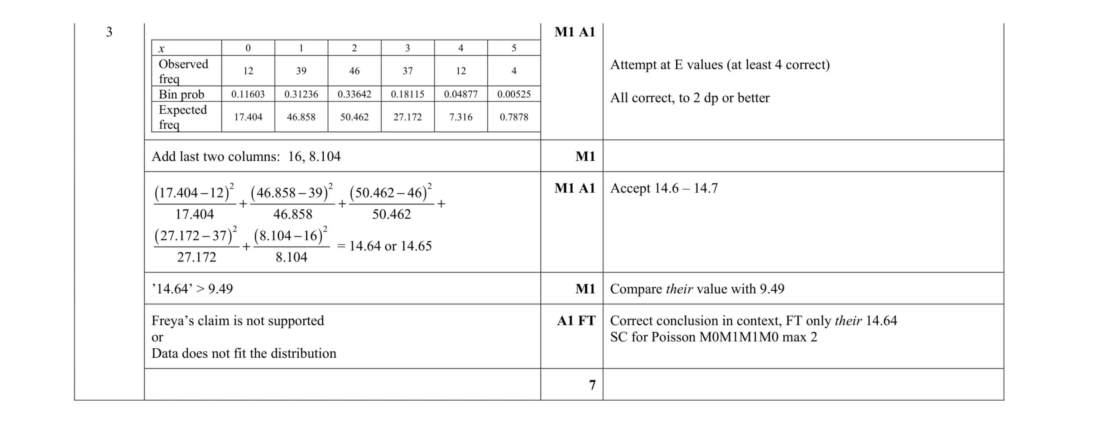 7
7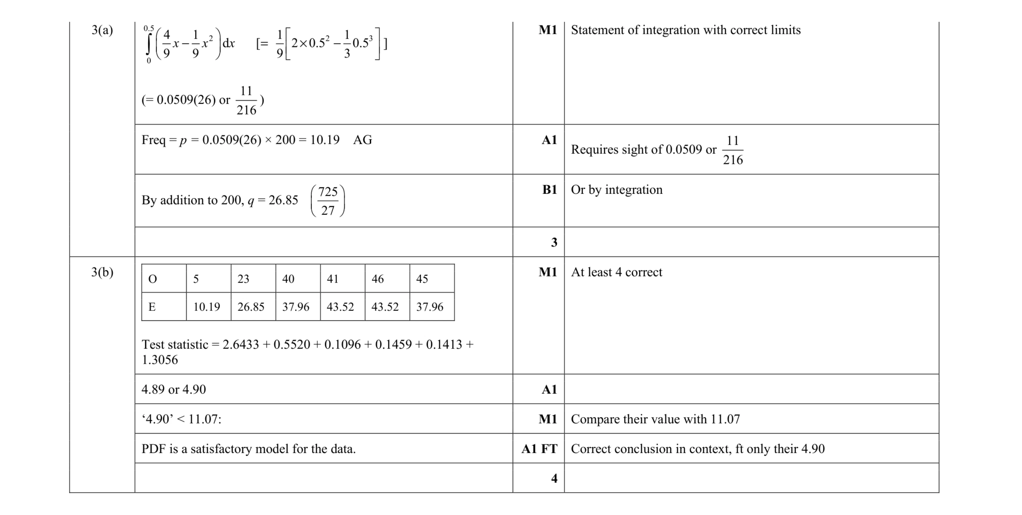 7
7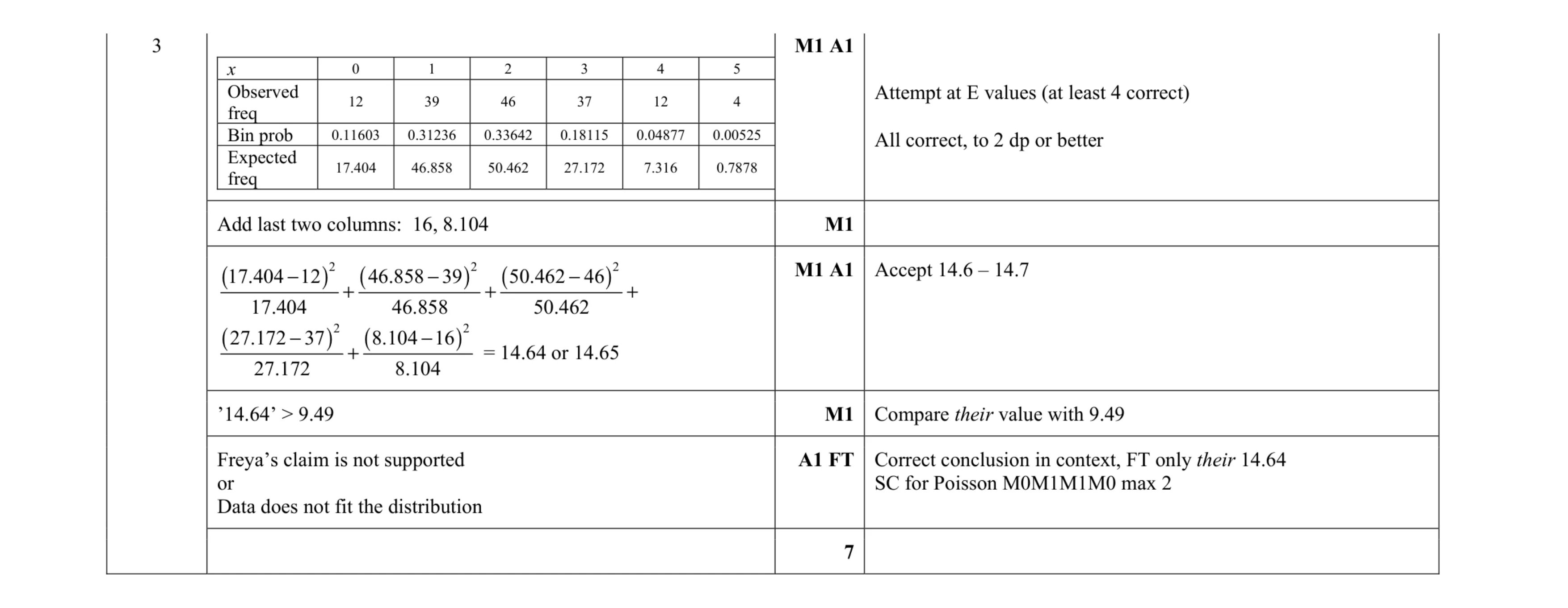 7
7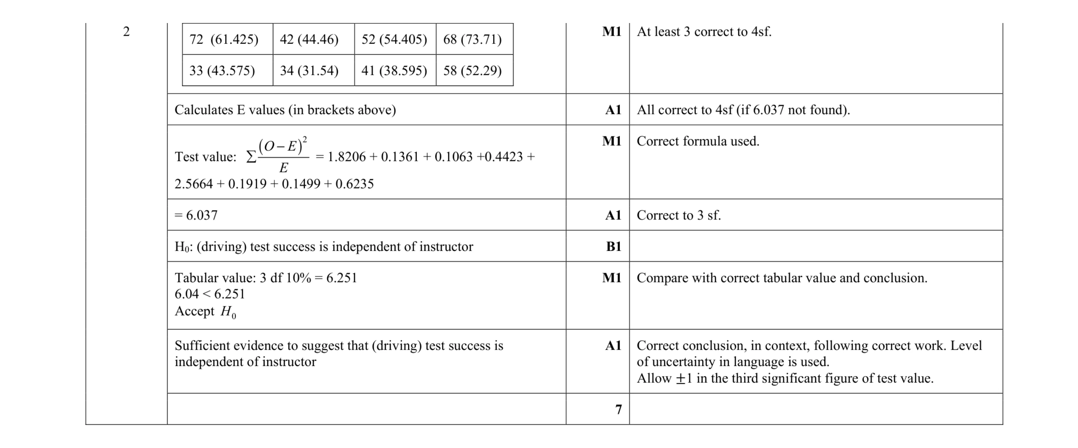 7
7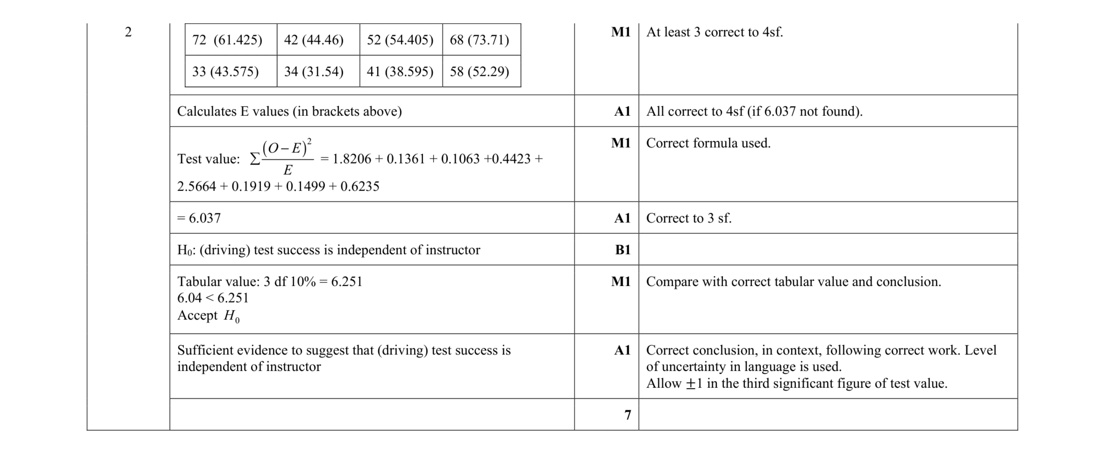 7
7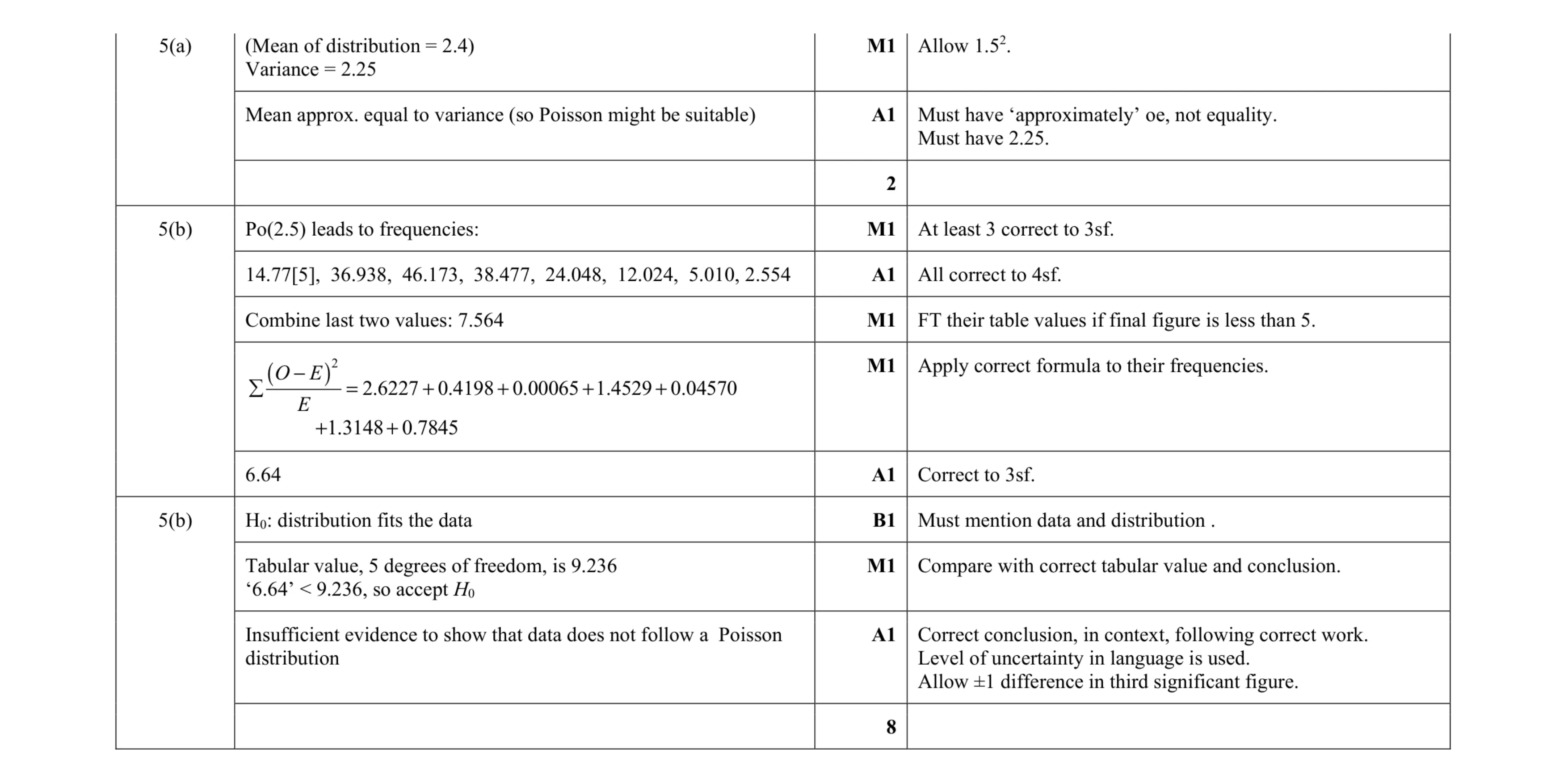 10
10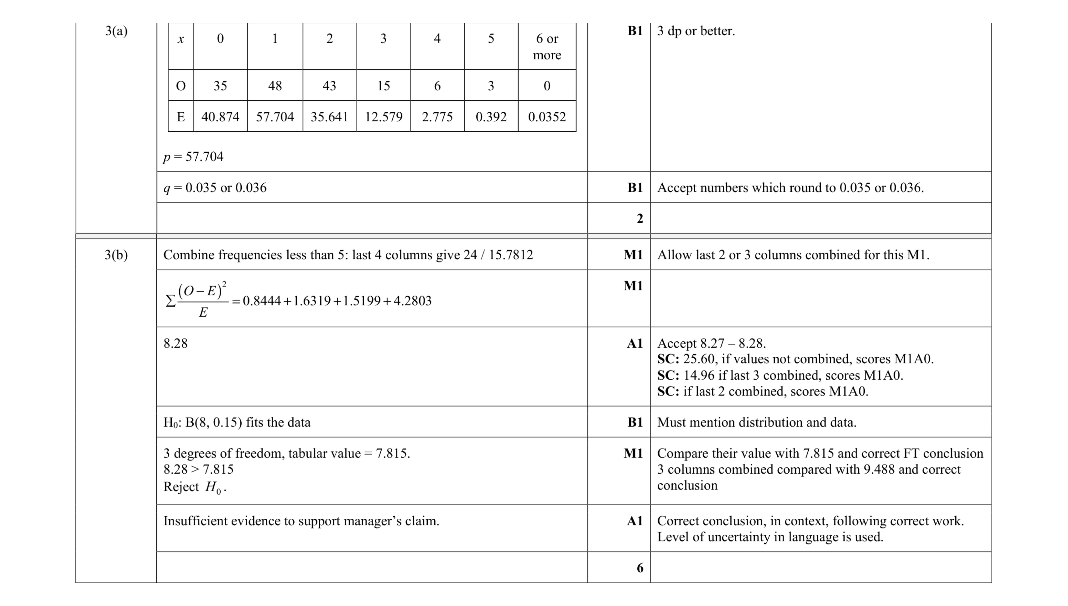 8
8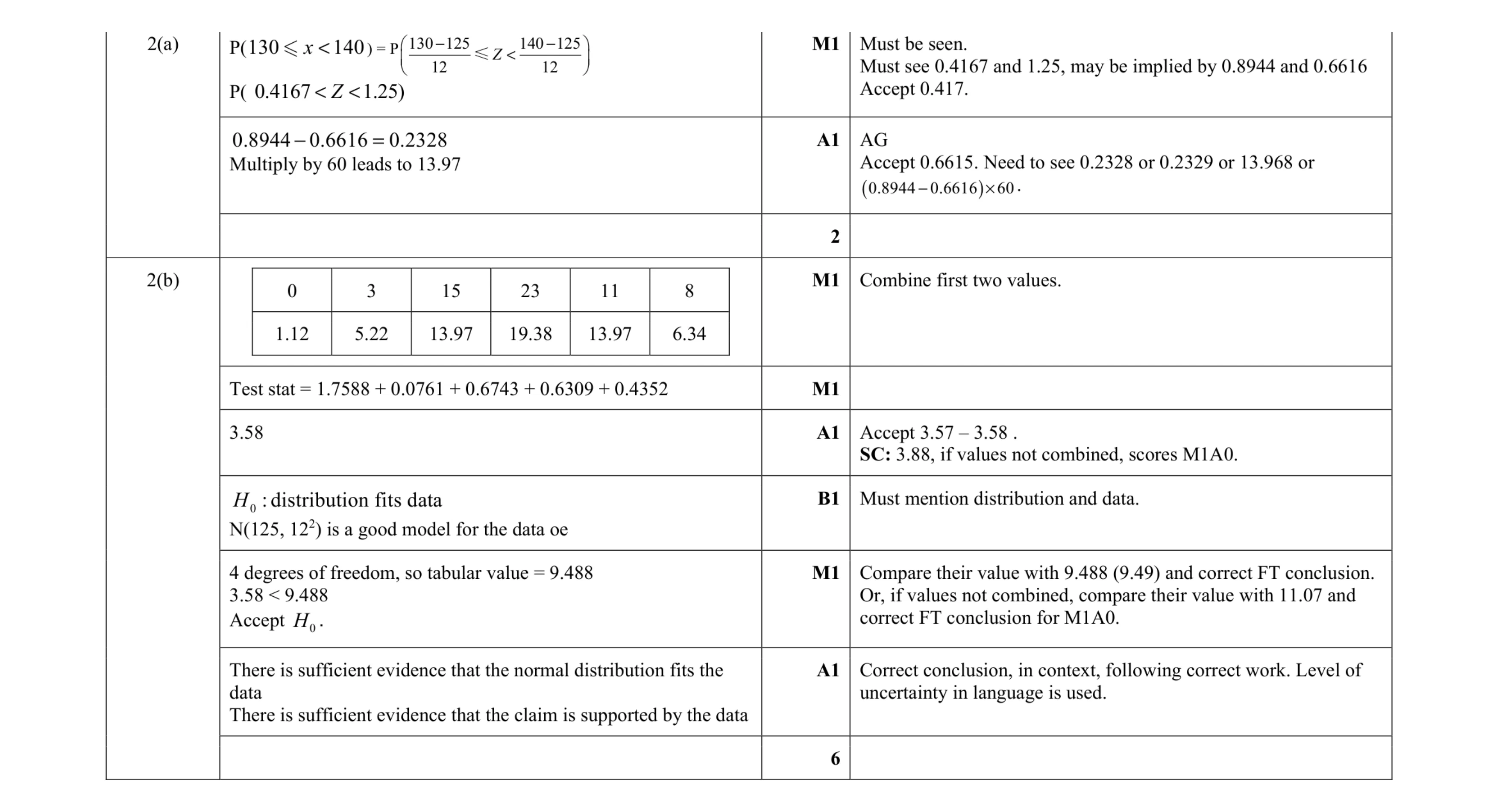 8
8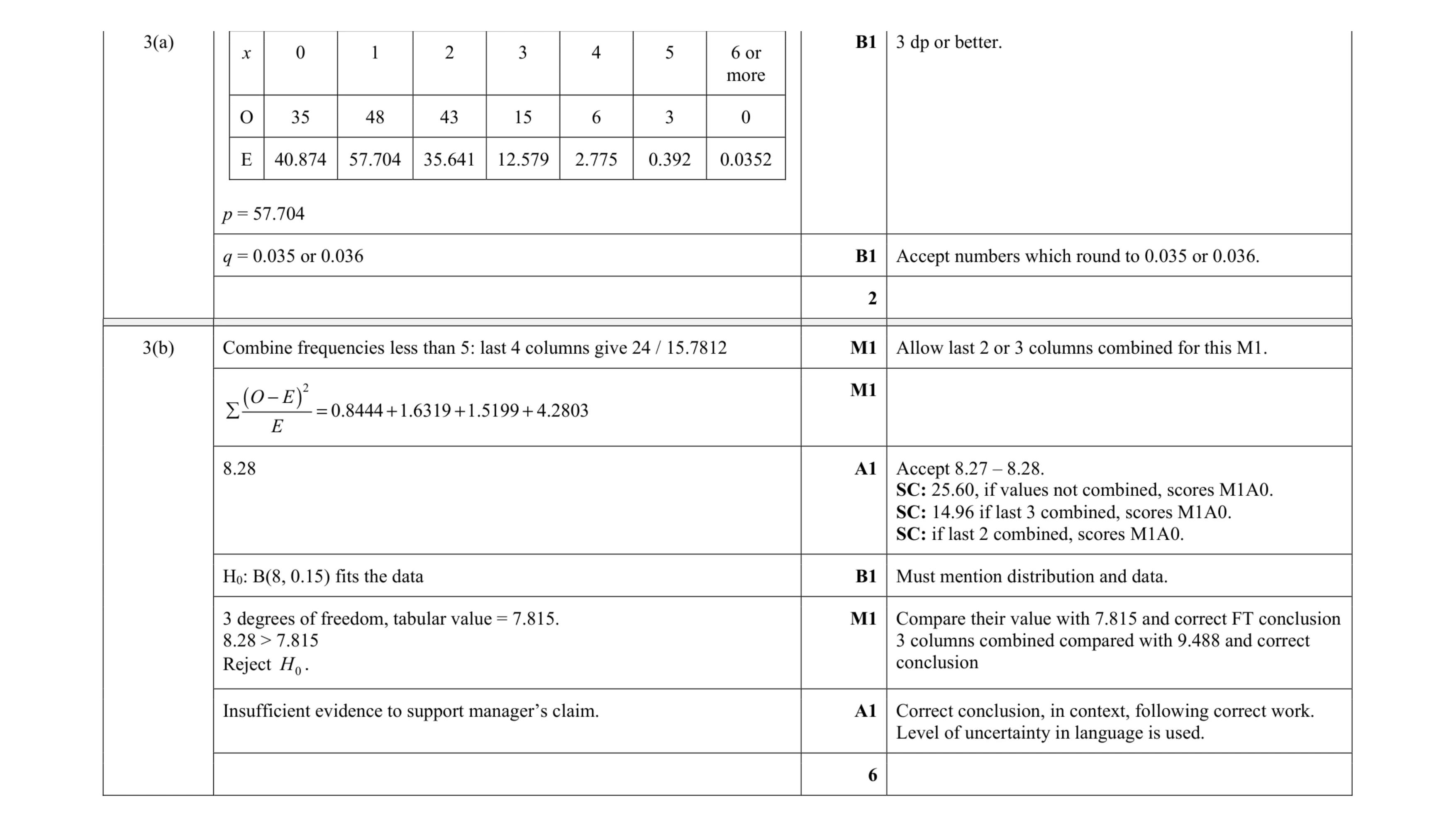 8
8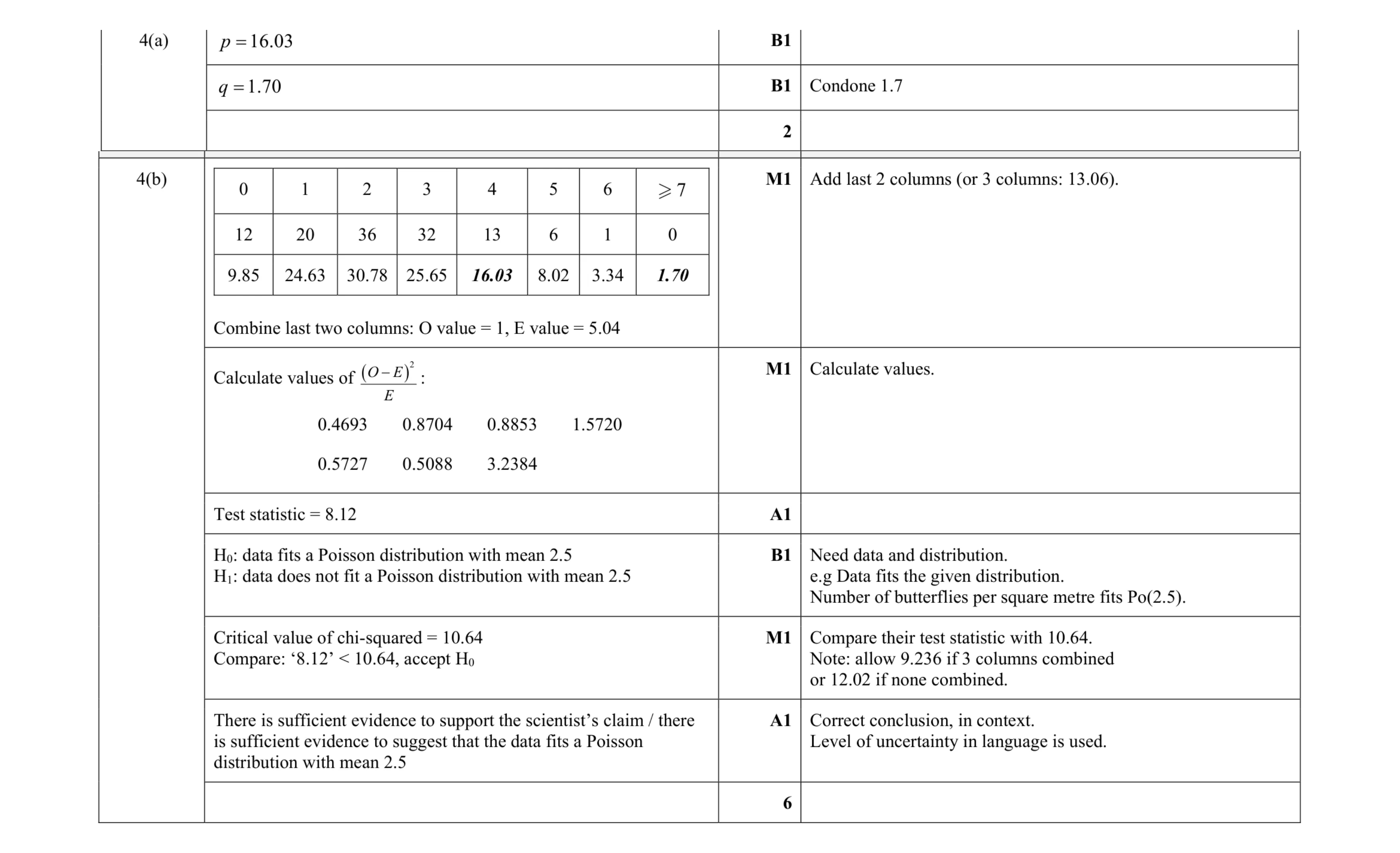 8
8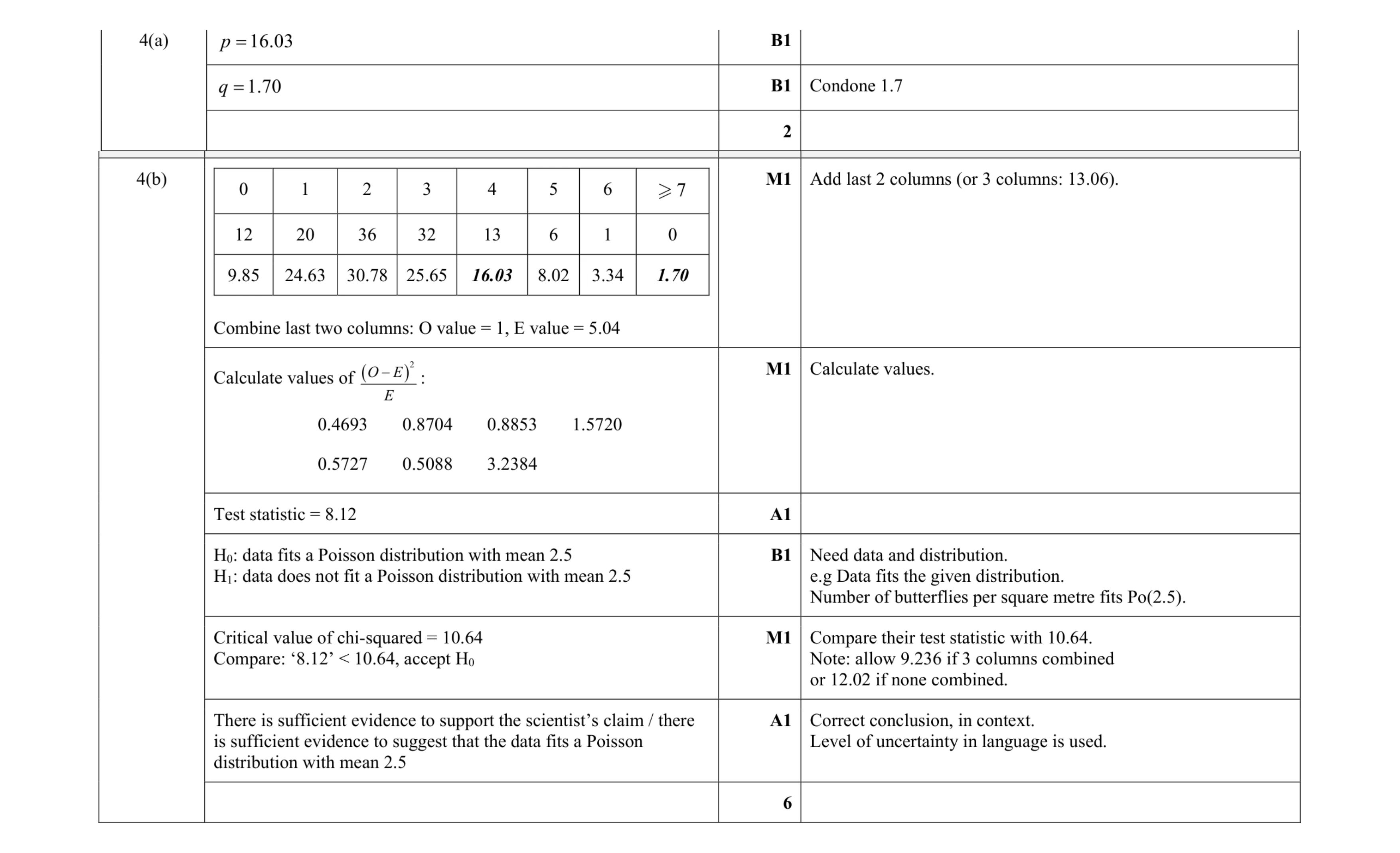 8
8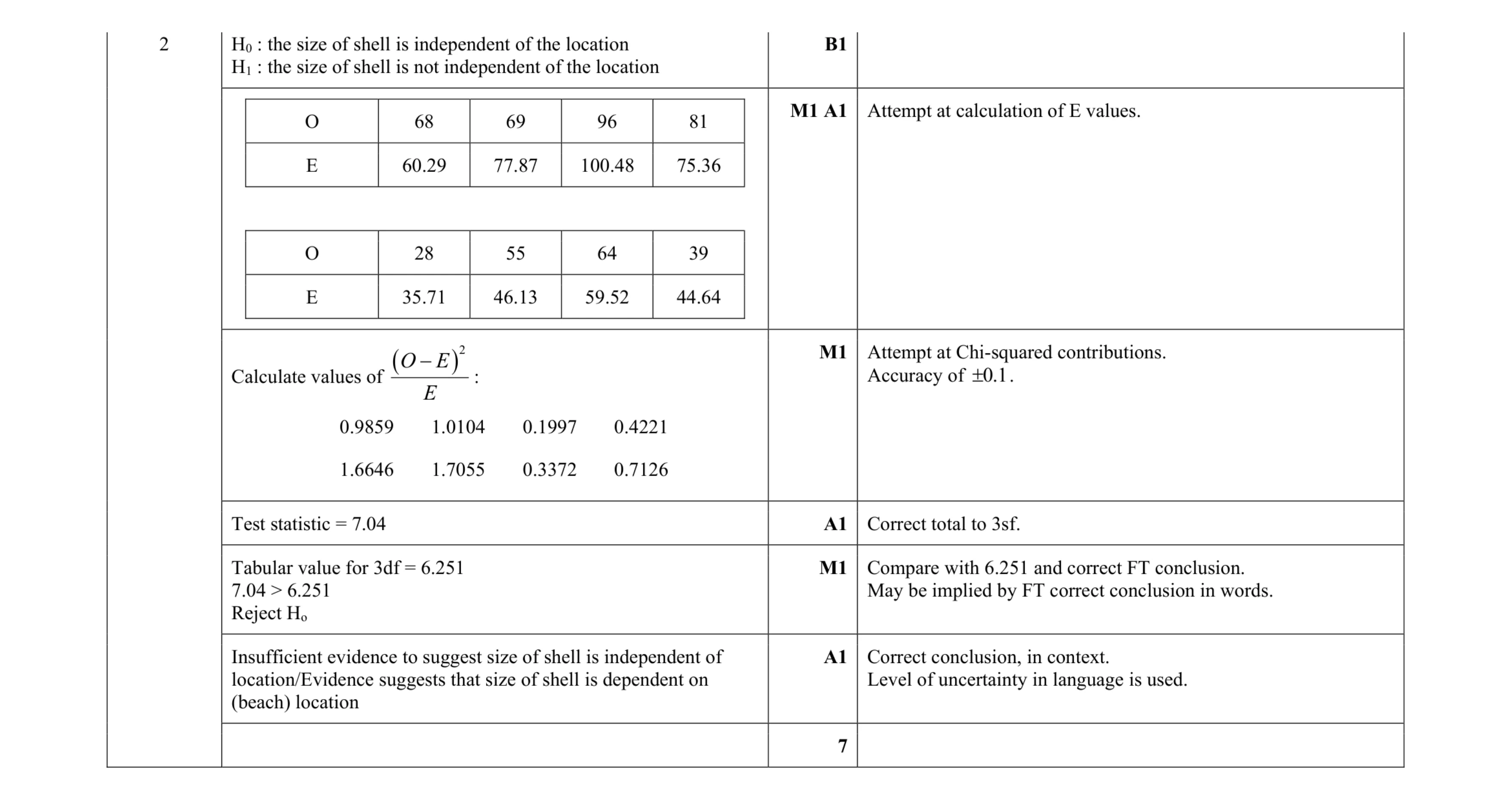 7
7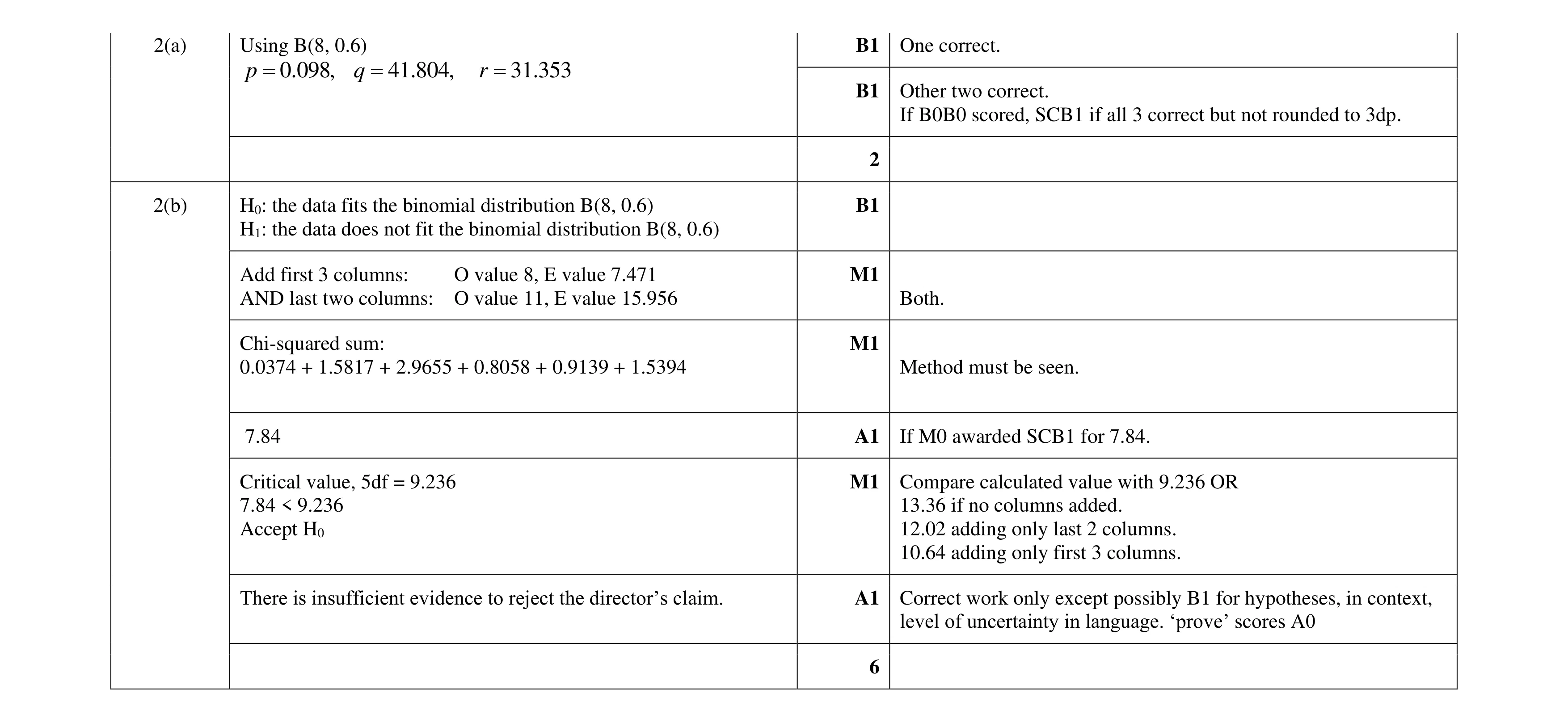 8
8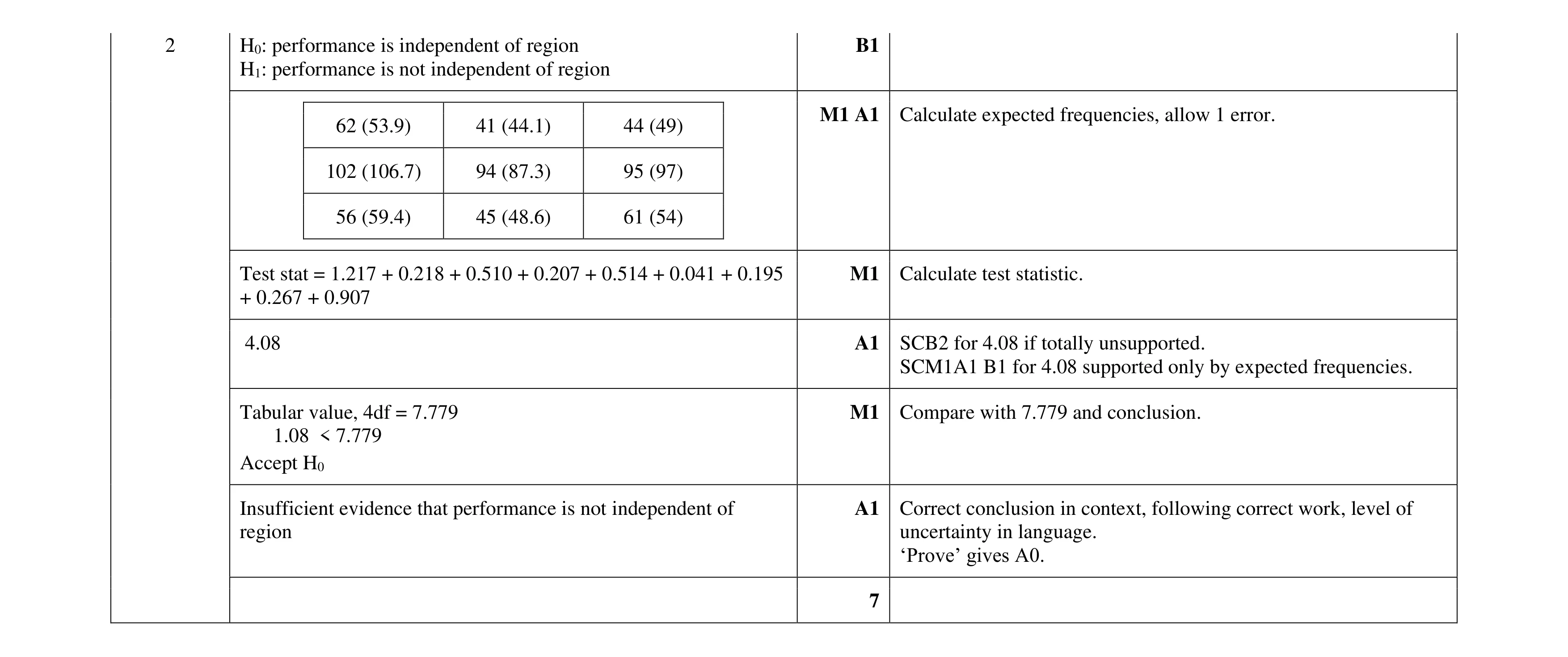 7
7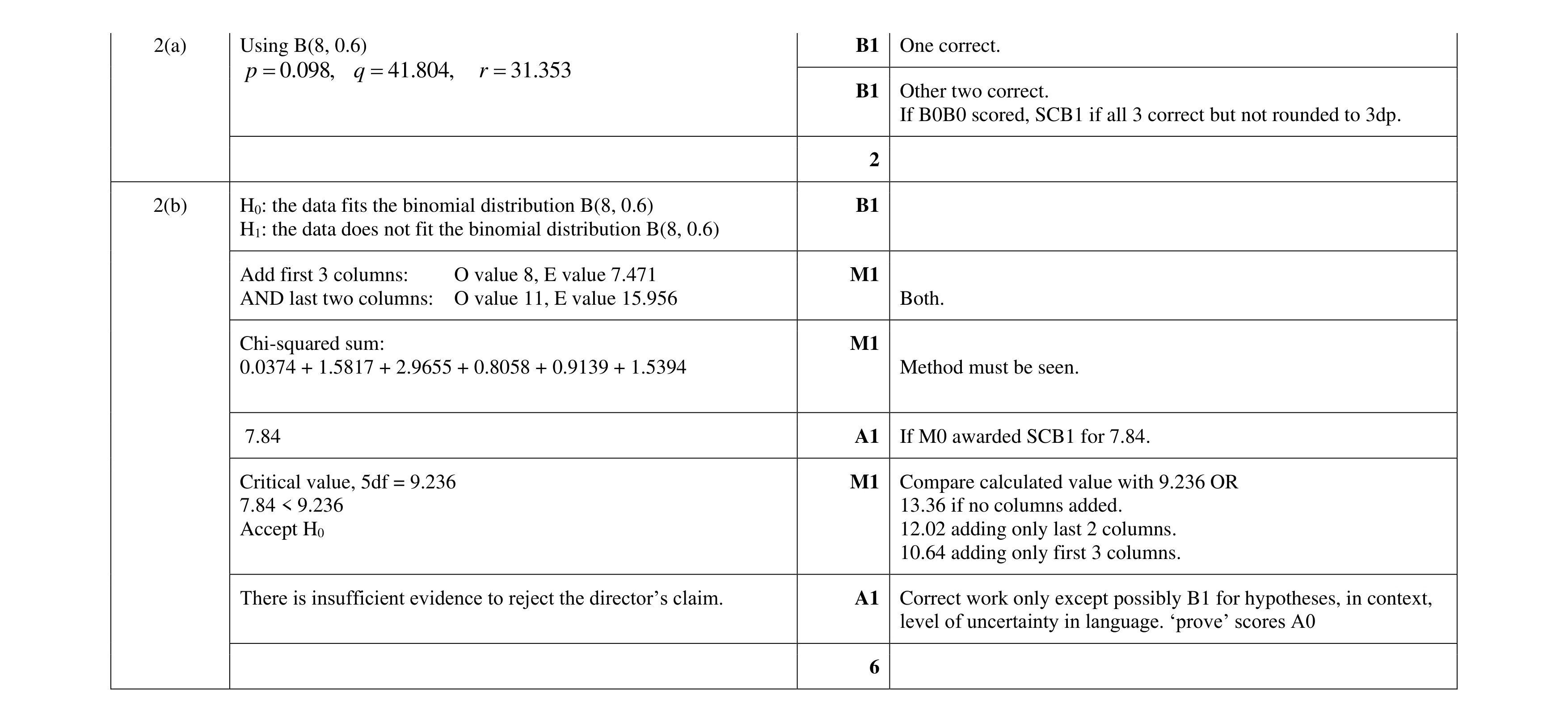 8
8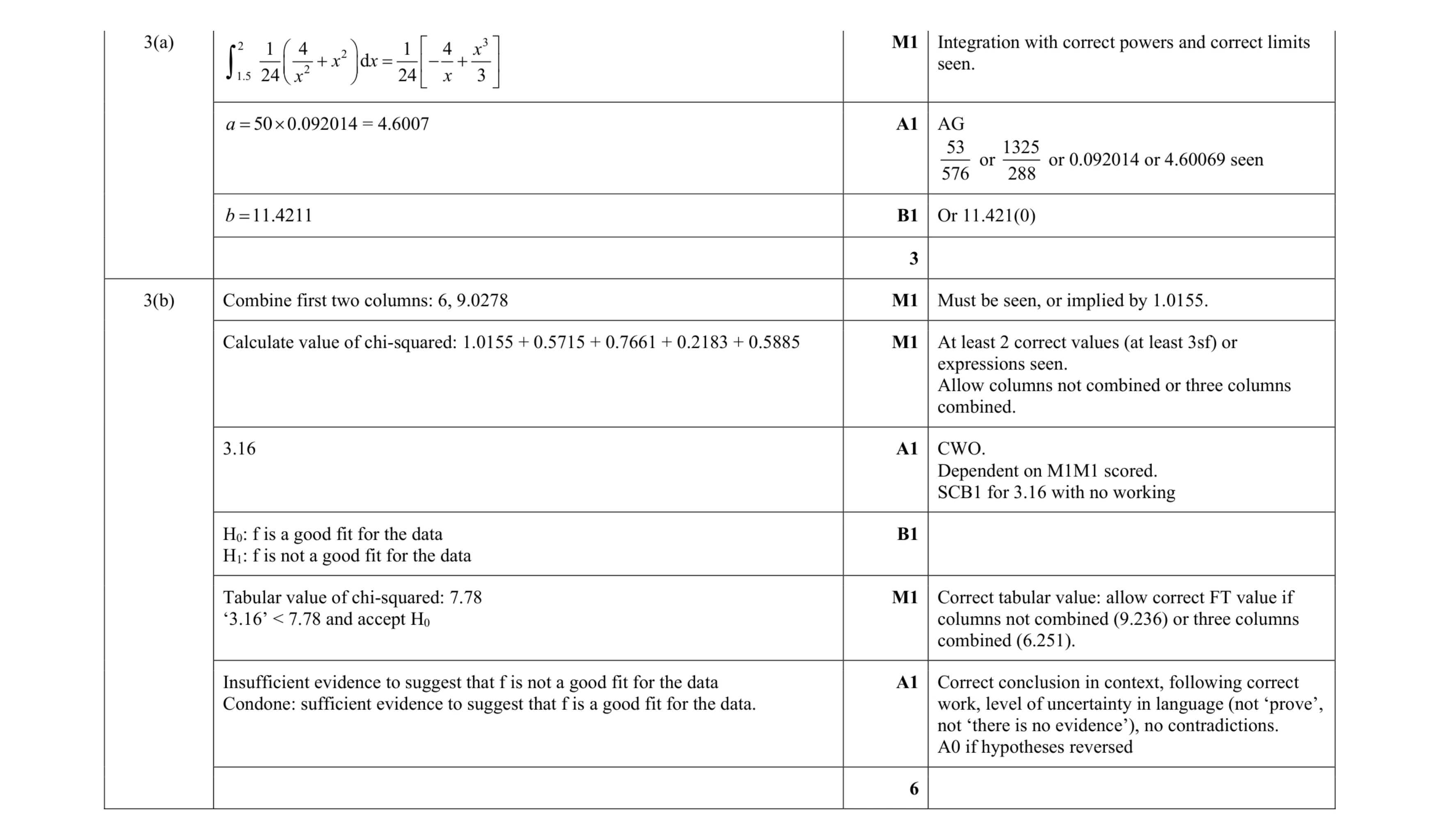 9
9 9
9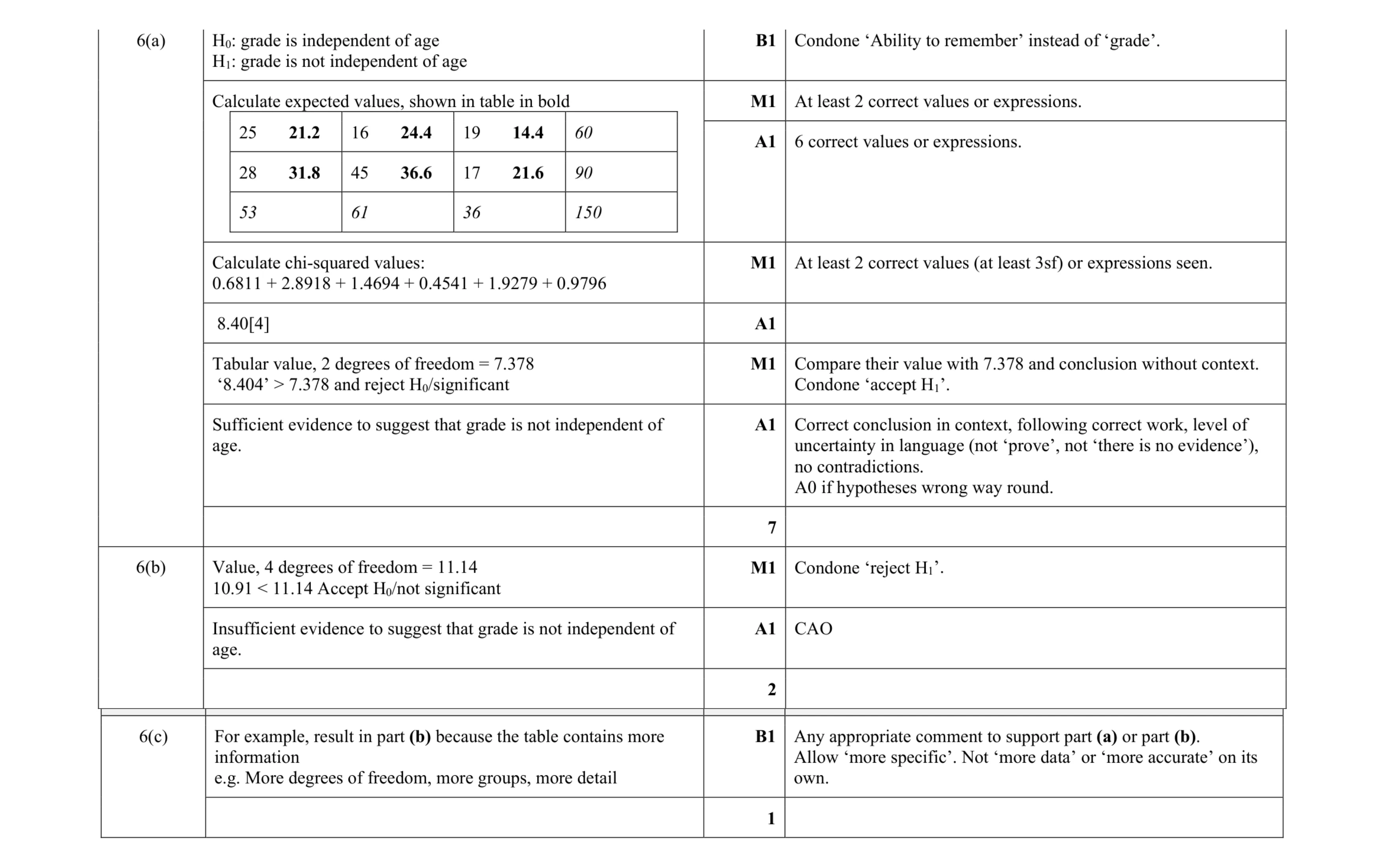 10
10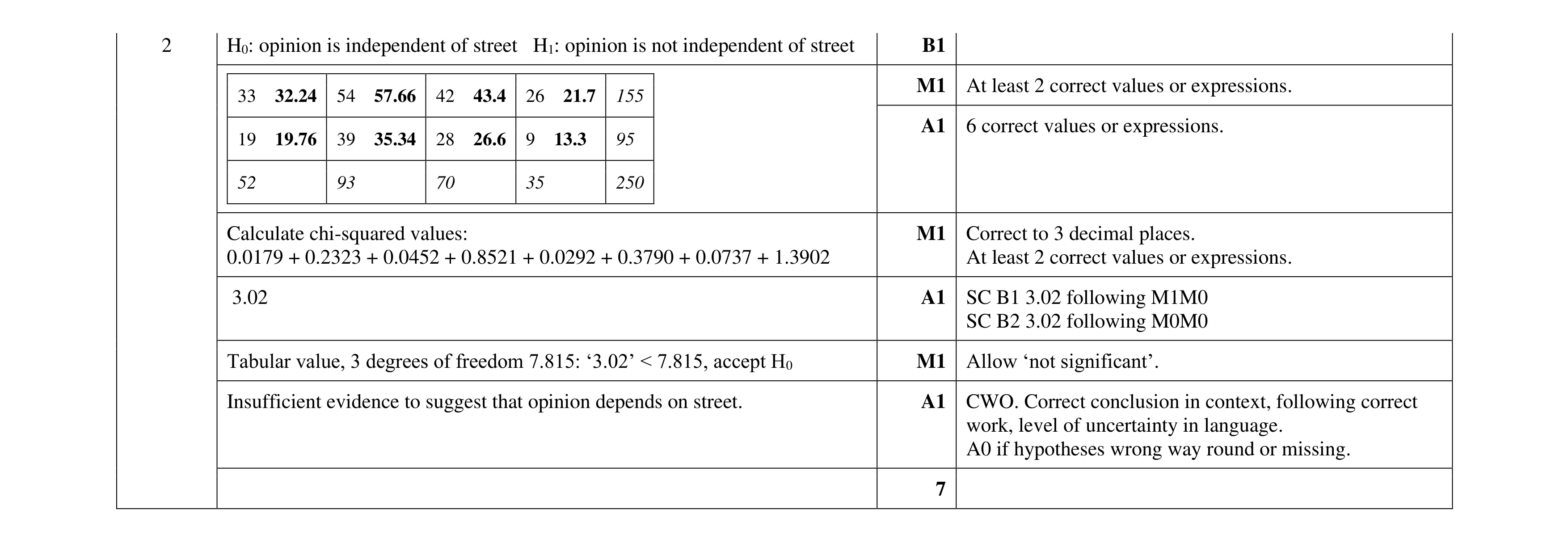 7
7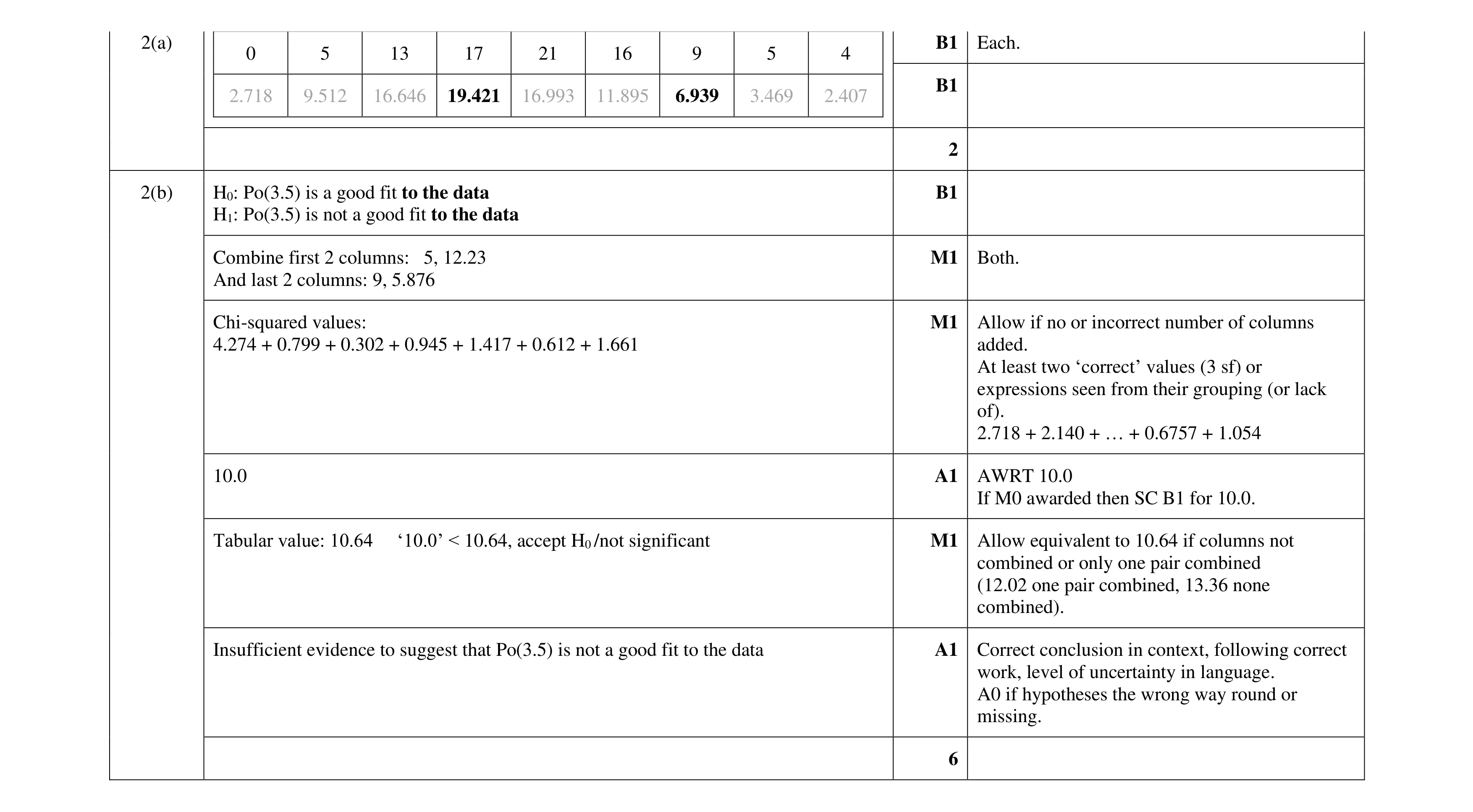 8
8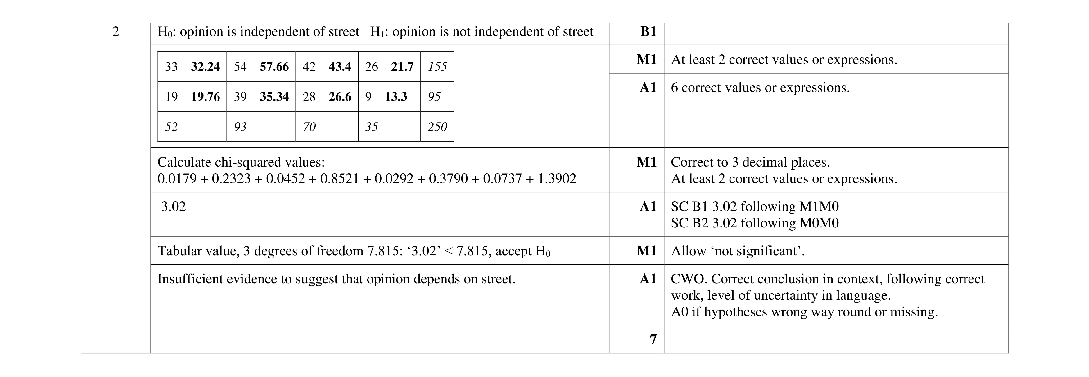 7
7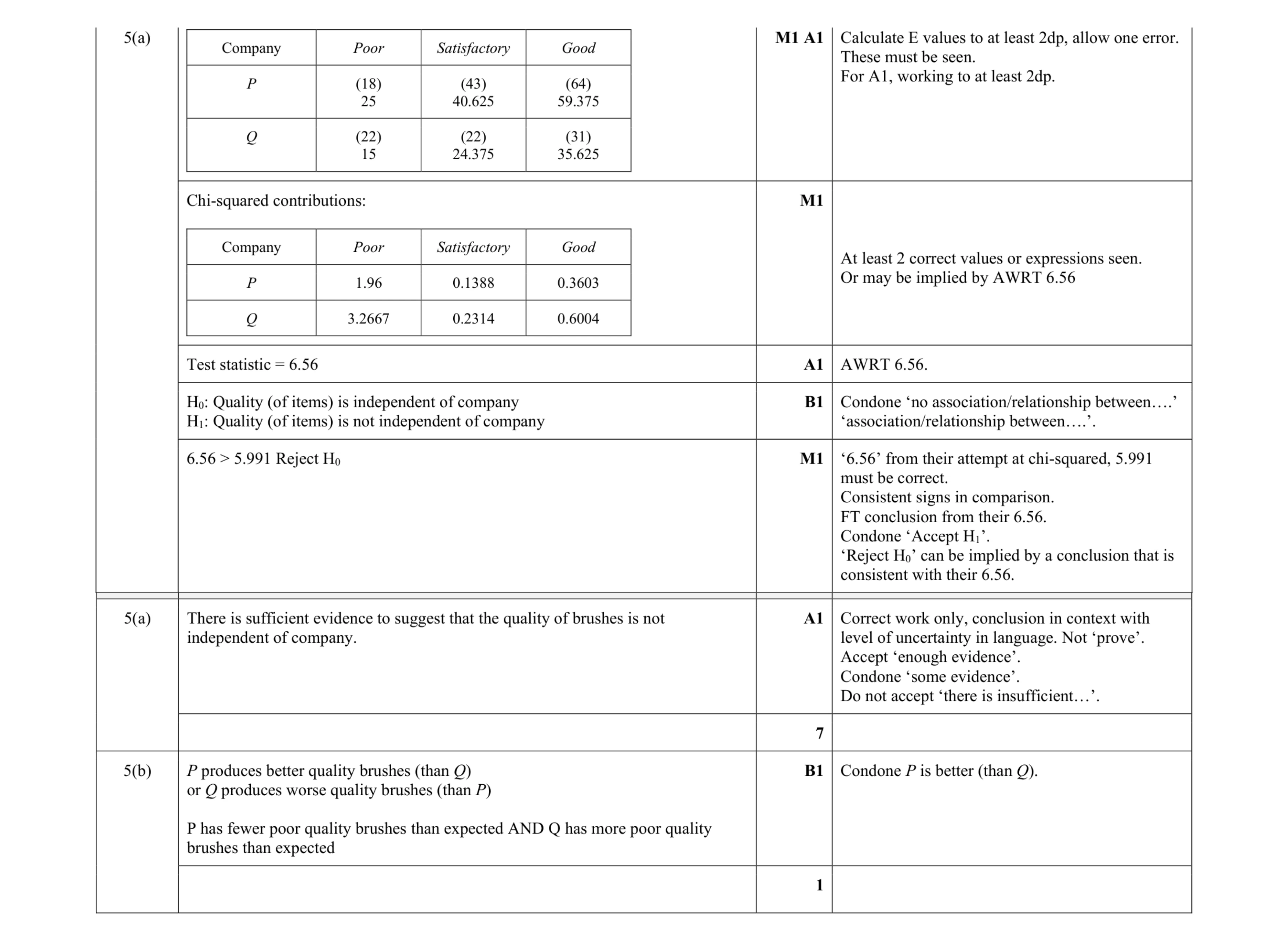 8
8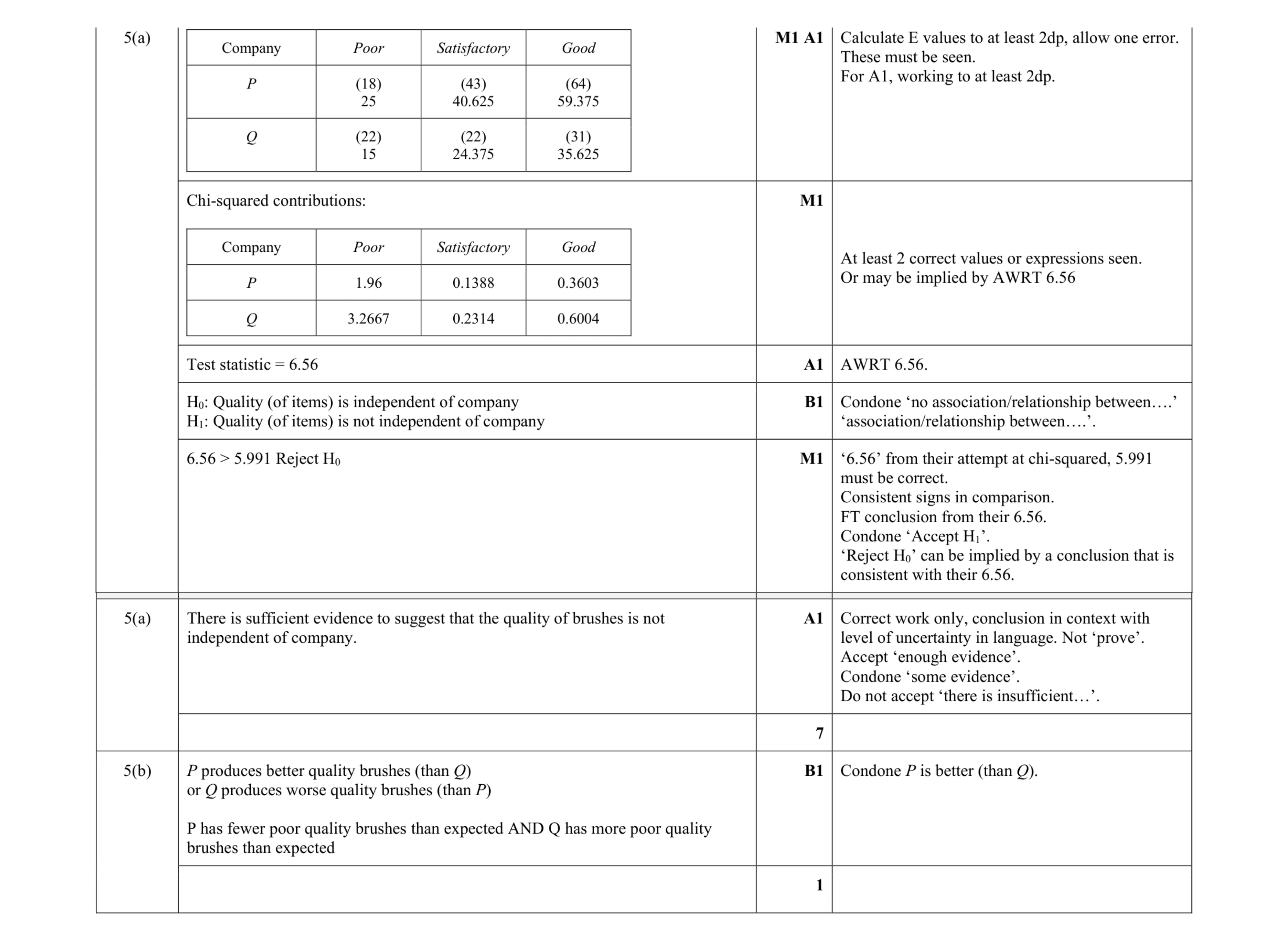 8
8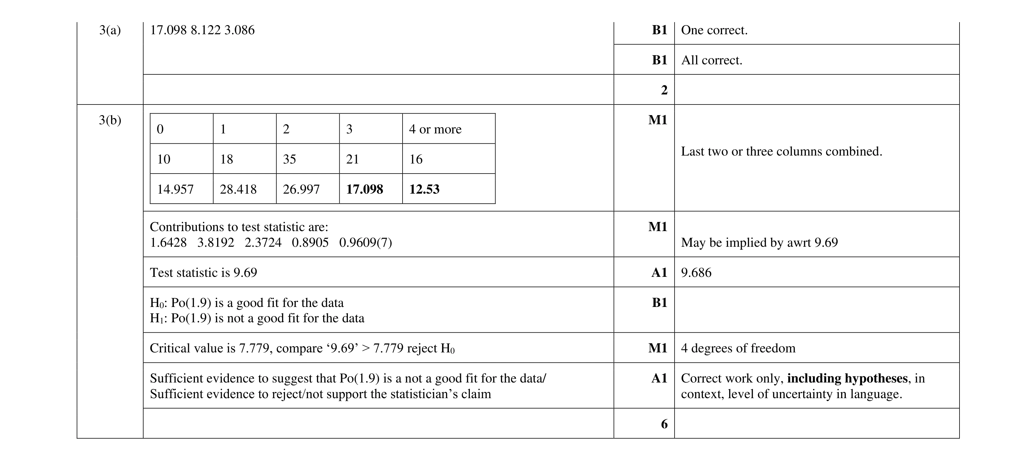 8
8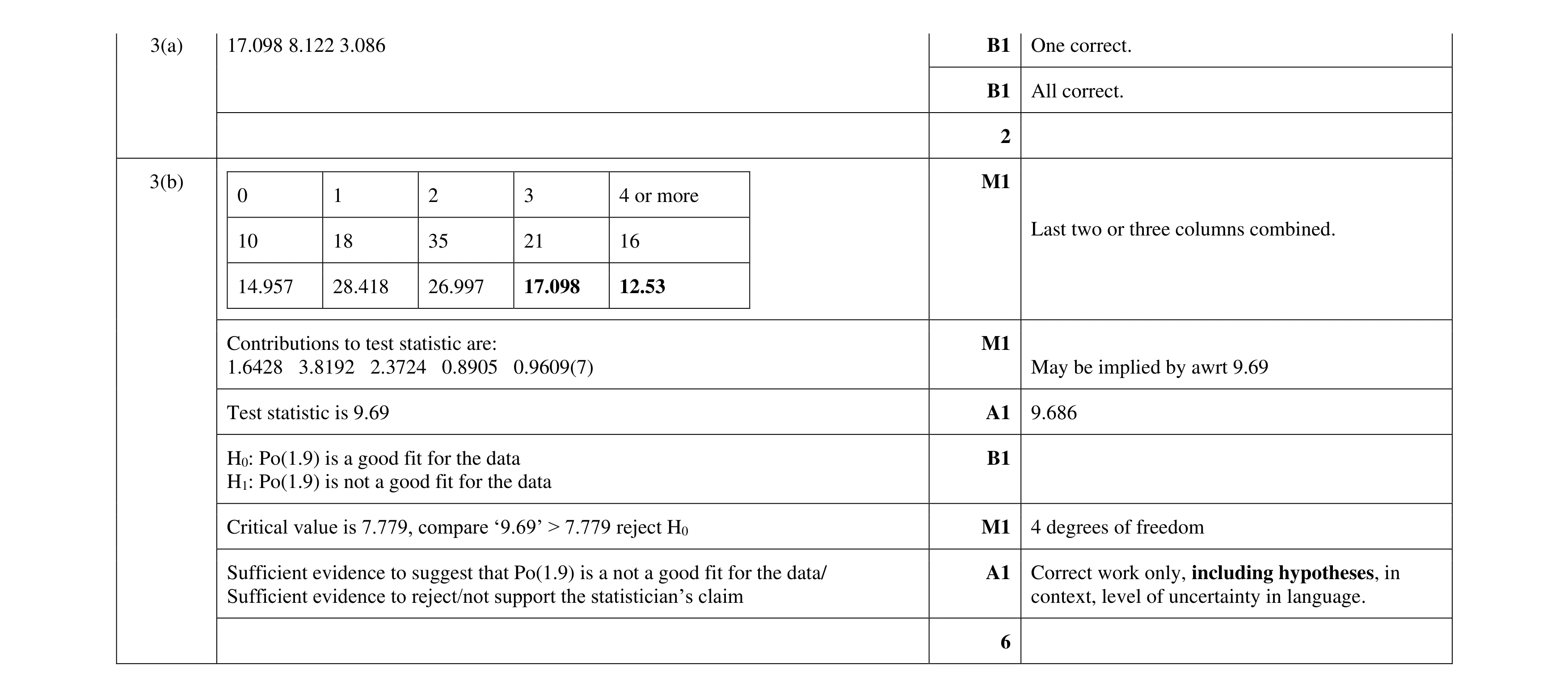 8
8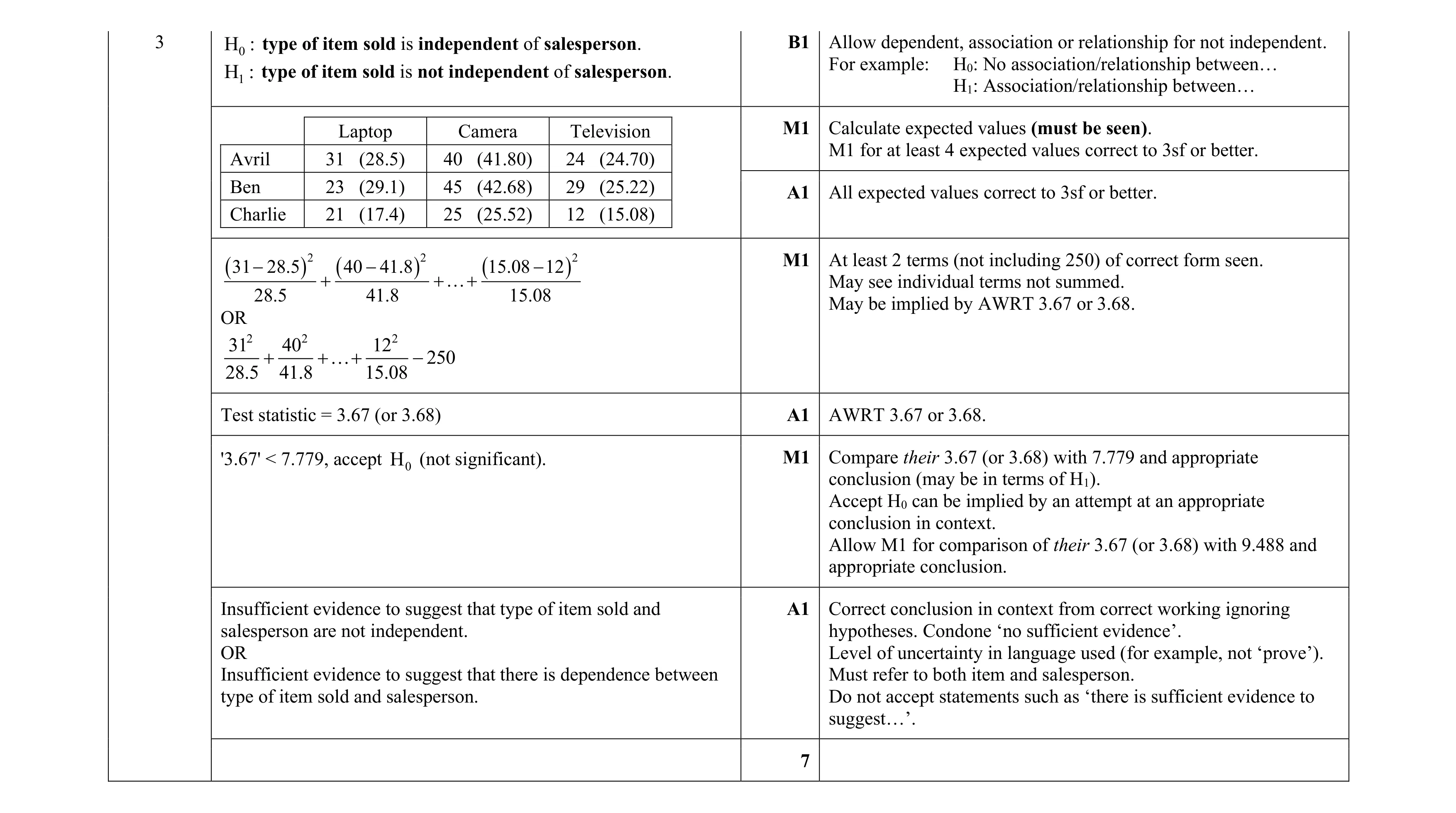 7
7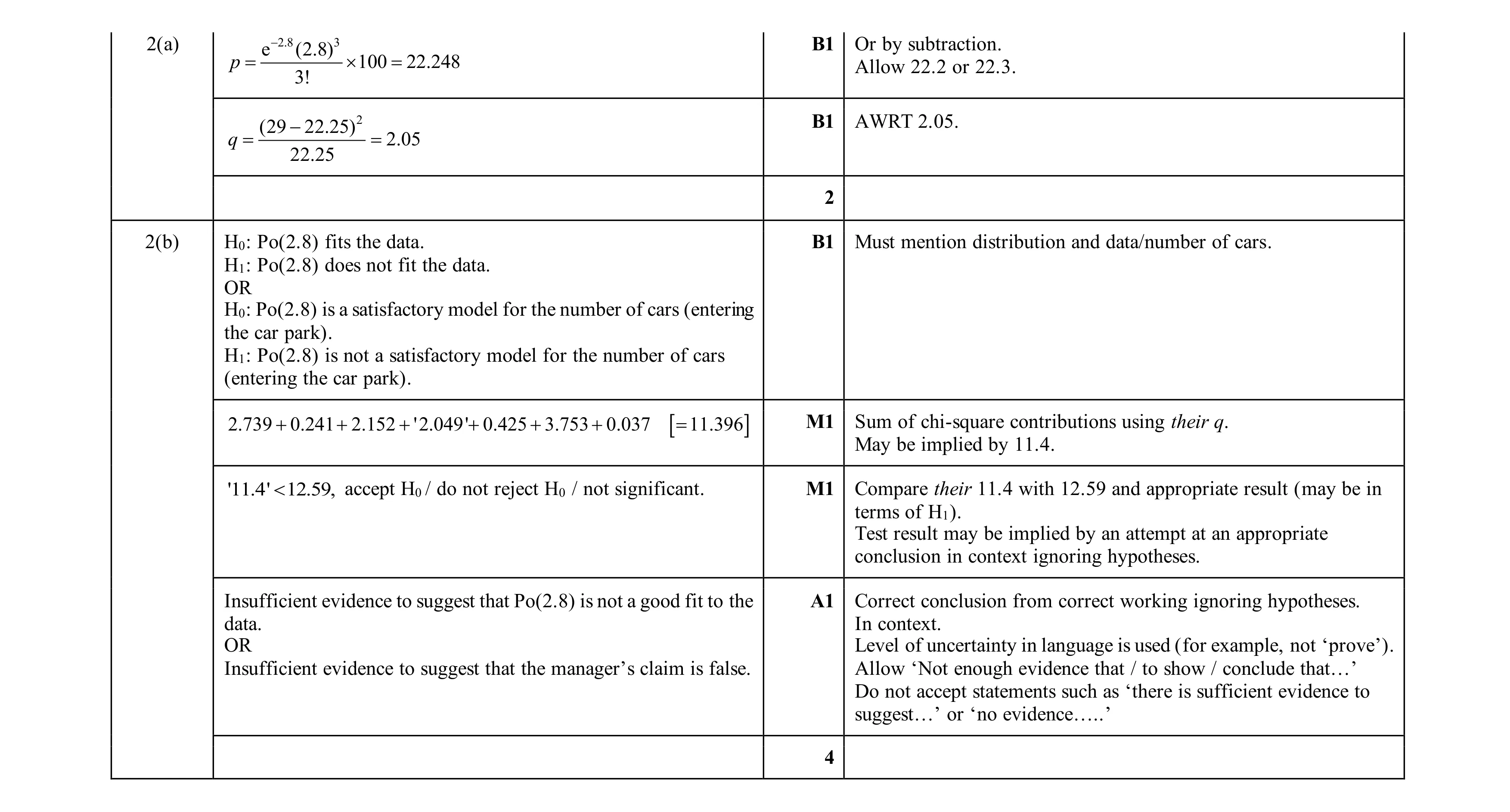 6
6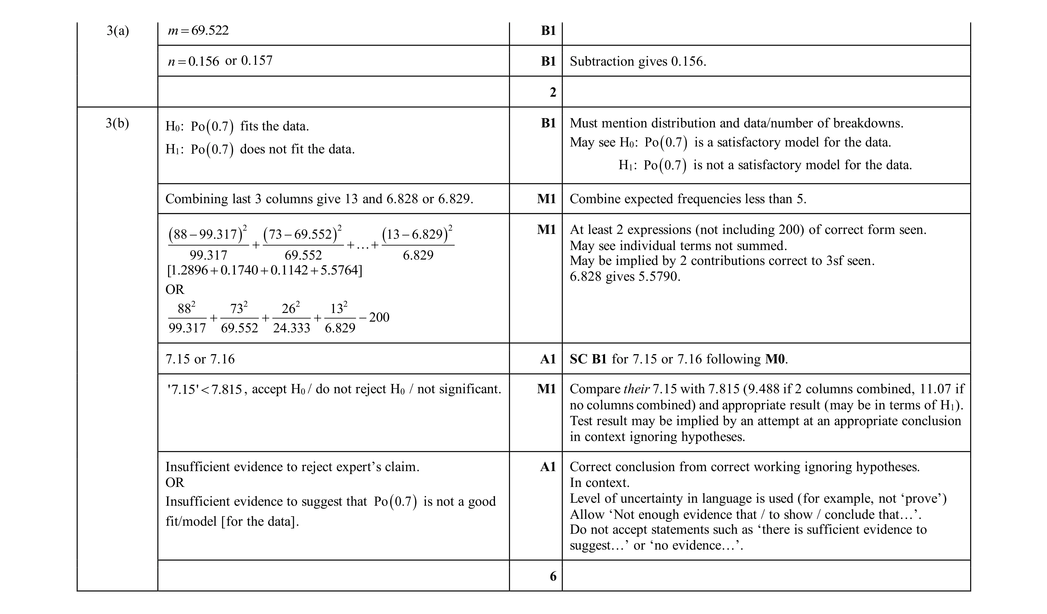 8
8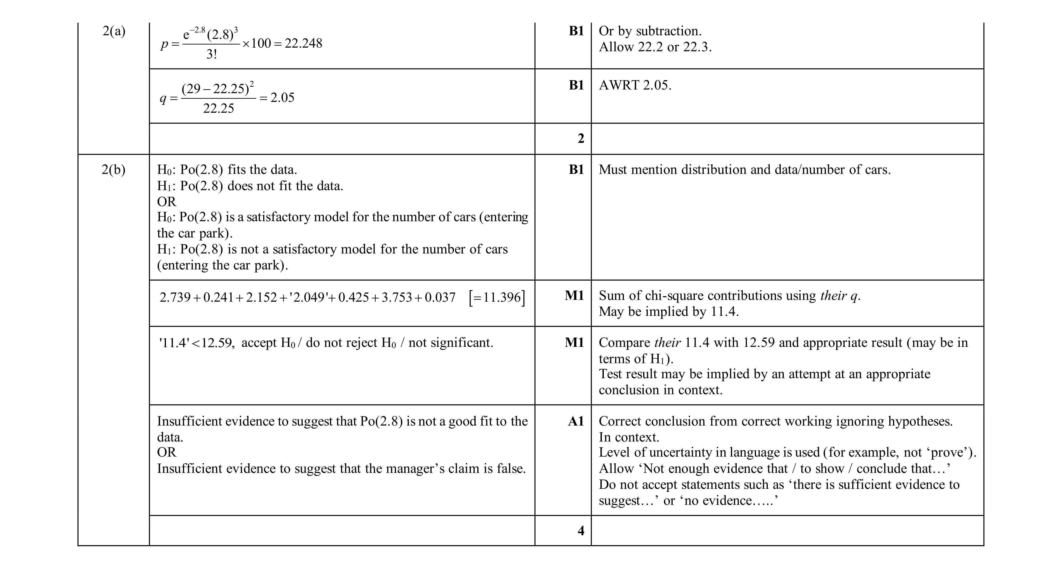 6
6