Questions as text
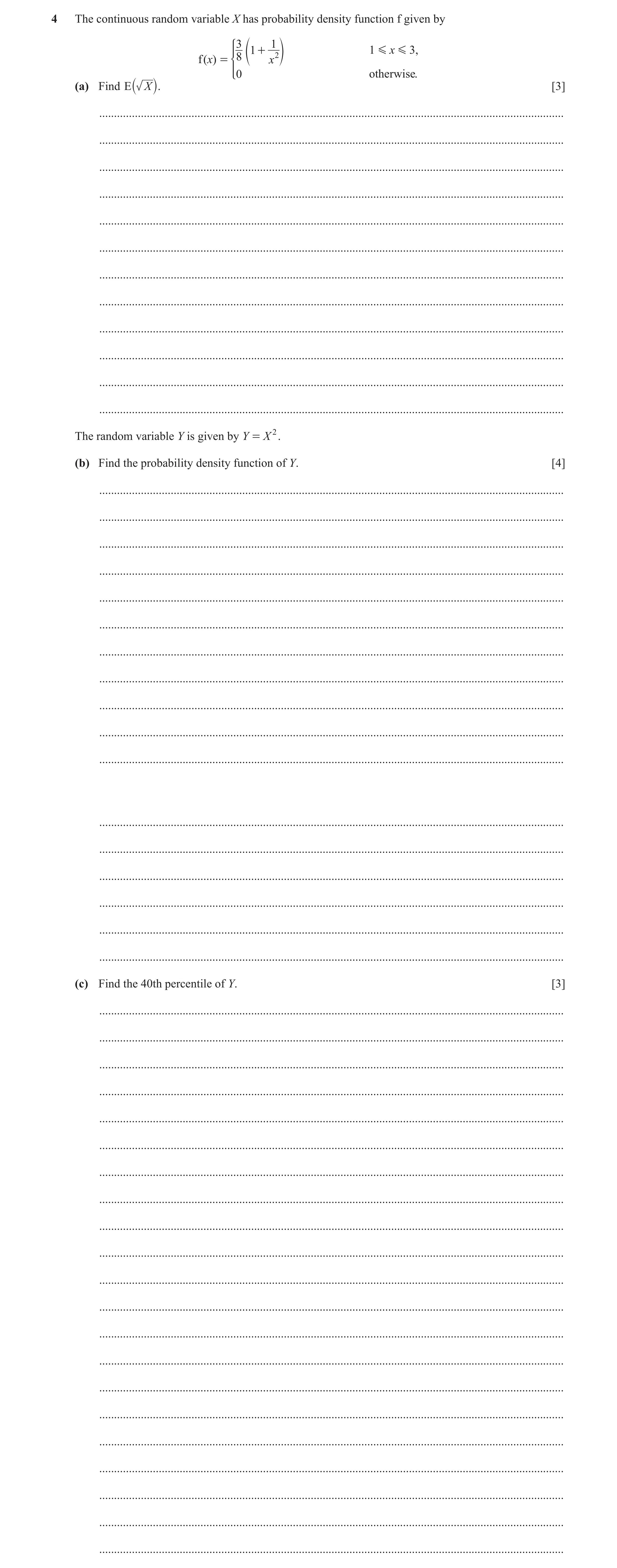
Q1 · The continuous random variable X has probability density function f given by Z 3 ] 16 2… 9231/41 May/June 2020
3 The continuous random variable X has probability density function f given by Z 3 ] 16 2 - x 0 G x 1 1, ` j ] 3 f ( x) = [ 1 G x G 9, 16 x ]] 0 otherwise. \ (a) Find E(X). [3] … … … … … … … … … … … … … … … … … … … … … … … The random variable Y is such that Y = X . (b) Find the probability density function of Y. [5] … … … … … … … … … … … … … … … … … … … … … … … … … …
8 marks
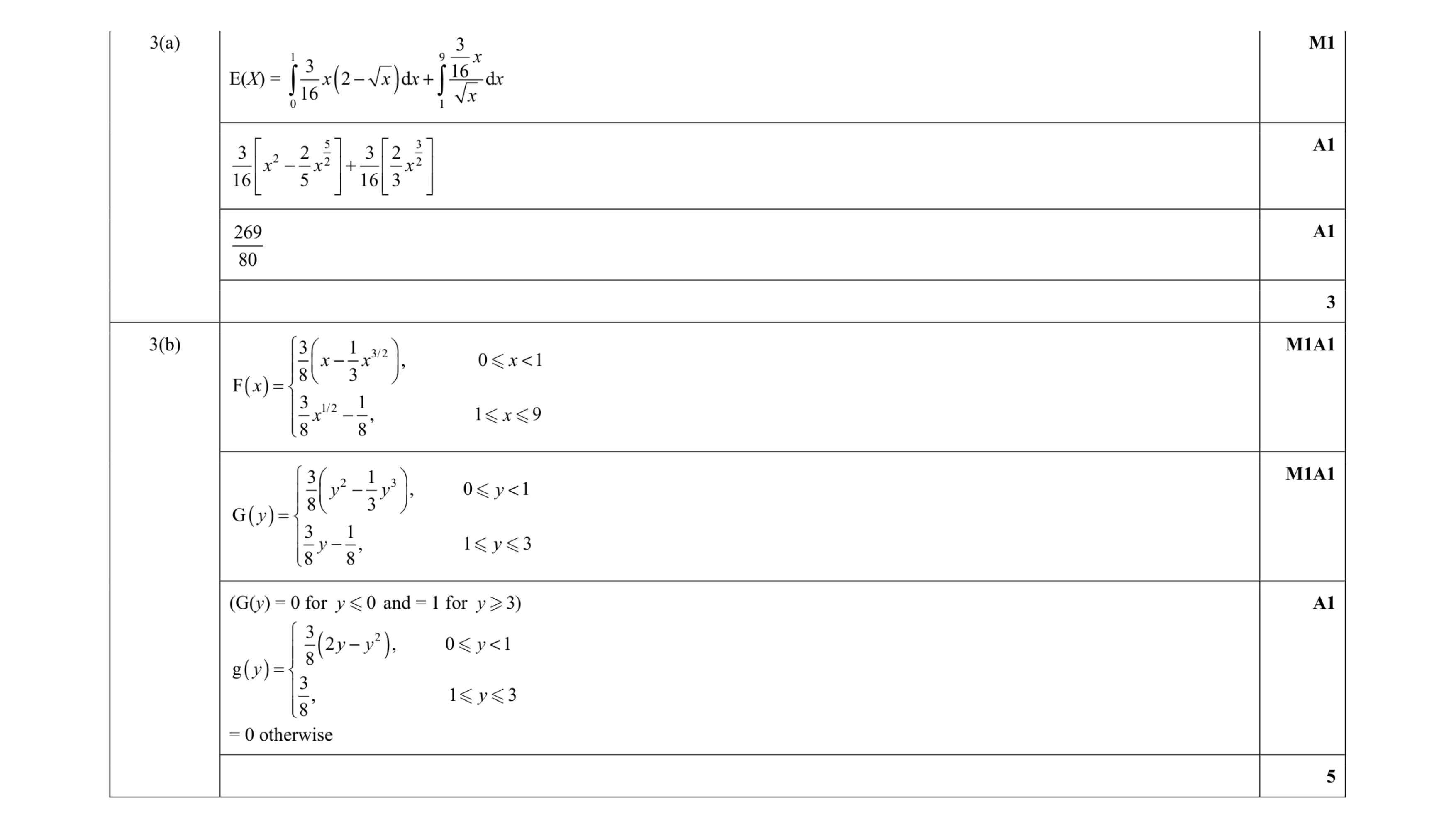
Mark scheme: 3(a) E(X) = ( ) 1 9 0 1 3 3 16 2 d d 16 − + x x x x x x M1 5 3 2 2 2 3 2 3 2 16 5 16 3 x x x − + A1 269 80 A1 3 3(b) ( ) 3/2 1/2 3 1 , 0 1 8 3 F 3 1, 1 9 8 8 − < = − x x x x x x M1A1 ( ) 2 3 3 1 , 0 1 8 3 G 3 1, 1 3 8 8 − < = − y y y y y y M1A1 (G(y) = 0 for 0 y and = 1 for 3) y ( ) ( ) 2 3 2 , 0 1 8 g 3, 1 3 8 − < = y y y y y = 0 otherwise A1 5
This question in 9231/41 May/June 2020
Q2 · The continuous random variable X has probability density function f given by Z 3 ] 16 2… 9231/42 May/June 2020
3 The continuous random variable X has probability density function f given by Z 3 ] 16 2 - x 0 G x 1 1, ` j ] 3 f ( x) = [ 1 G x G 9, 16 x ]] 0 otherwise. \ (a) Find E(X). [3] … … … … … … … … … … … … … … … … … … … … … … … The random variable Y is such that Y = X . (b) Find the probability density function of Y. [5] … … … … … … … … … … … … … … … … … … … … … … … … … …
8 marks
Mark scheme: 3(a) E(X) = ( ) 1 9 0 1 3 3 16 2 d d 16 − + x x x x x x 5 3 2 2 2 3 2 3 2 16 5 16 3 x x x − + A1 269 80 A1 3 3(b) ( ) 3/2 1/2 3 1 , 0 1 8 3 F 3 1, 1 9 8 8 − < = − x x x x x x M1A1 ( ) 2 3 3 1 , 0 1 8 3 G 3 1, 1 3 8 8 − < = − y y y y y y M1A1 (G(y) = 0 for 0 y and = 1 for 3) y ( ) ( ) 2 3 2 , 0 1 8 g 3, 1 3 8 − < = y y y y y = 0 otherwise A1 5
This question in 9231/42 May/June 2020
Q3 · The continuous random variable X has probability density function f given by 1 5 x 0 G x… 9231/43 May/June 2020
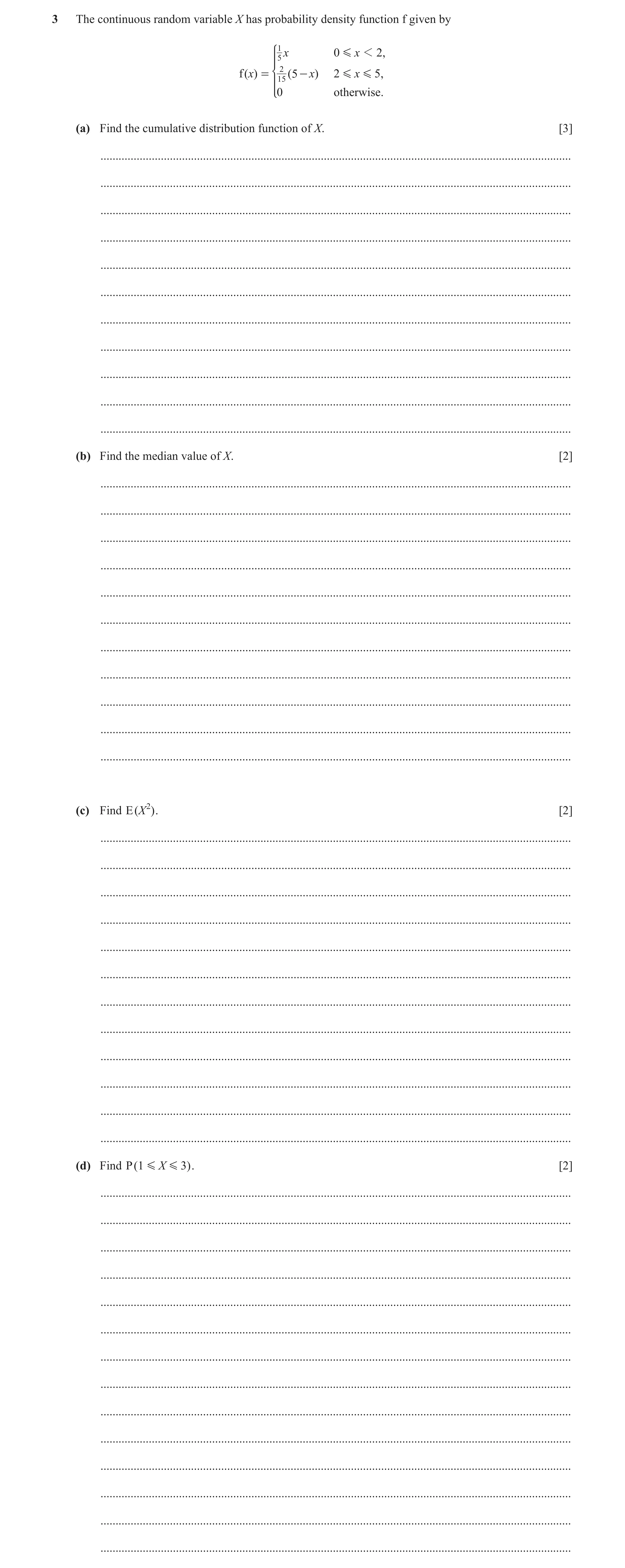
3 The continuous random variable X has probability density function f given by 1 5 x 0 G x 1 2, - x) 2 G x G 5, f ( x) = 152 ( 5 *0 otherwise. (a) Find the cumulative distribution function of X. [3] … … … … … … … … … … … (b) Find the median value of X. [2] … … … … … … … … … … … (c) Find E ( X2 ) . [2] … … … … … … … … … … … … (d) Find P ( 1 G X G 3) . [2] … … … … … … … … … … … … … …
9 marks
Mark scheme: 3(a) ( ) ( ) 2 2 , 0 2 10 F 1 2 10 , 2 5 15 3 x x x x x x < = − − = 0 for x < 0 and = 1 for x > 5 A1 3 3(b) F(m) = ½ so 2 2 20 35 0 − + = m m M1 1 5 30 2.26 2 = − = m A1 2 3(c) E(X2) = ( ) 2 5 2 2 0 2 2 . d 5 . d 5 15 x x x x x x + − = 4 4 3 2 5 20 15 3 4 + − x x x M1 = 6.5 A1 2 Question Answer Marks 3(d) F(3) – F(1) M1 = 11 1 19 15 10 30 − = A1 Alternative method for 3(d) ( ) 2 3 2 2 1 2 2 2 d 5 d 5 5 15 10 15 2 + − = + − x x x x x x x M1 = 3 1 19 10 3 30 + = A1 2
This question in 9231/43 May/June 2020
Q4 · The continuous random variable X has cumulative distribution function F given by 0 x 1 0… 9231/41 Oct/Nov 2020
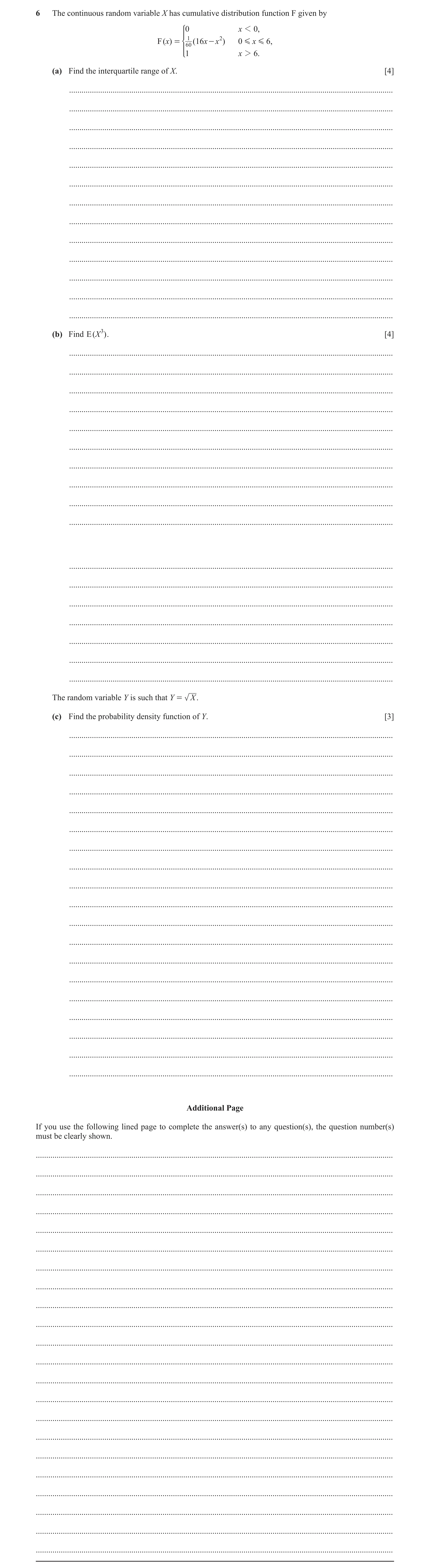
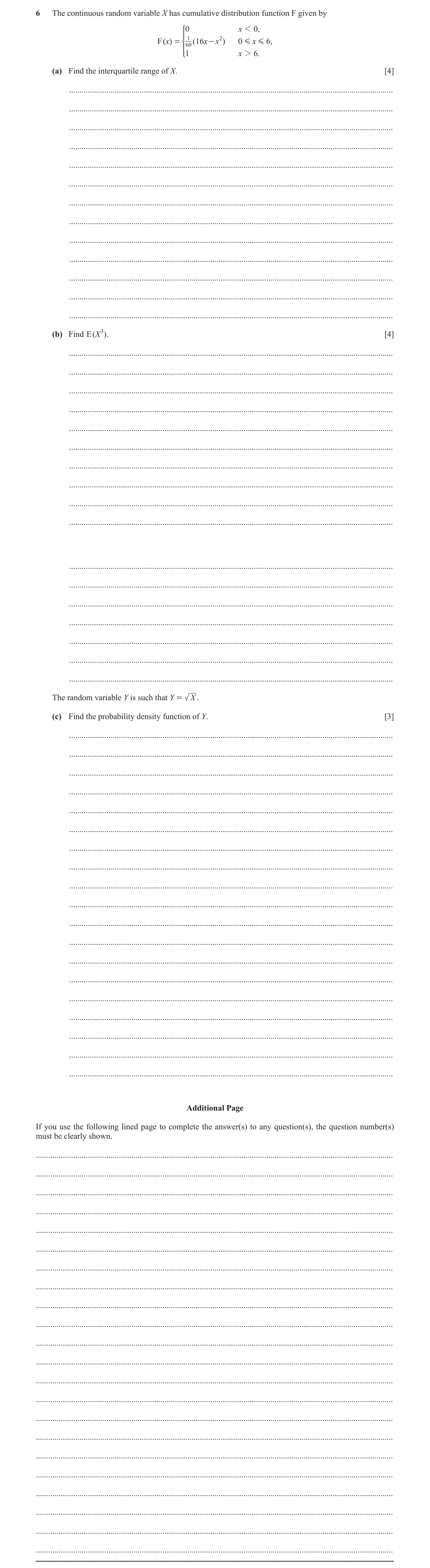
6 The continuous random variable X has cumulative distribution function F given by 0 x 1 0, - x ) 0 G x G 6, F ( x) = 601 ( 16 x 2 *1 x 2 6. (a) Find the interquartile range of X. [4] … … … … … … … … … … … … … (b) Find E ( X 3 ) . [4] … … … … … … … … … … … … … … … … … The random variable Y is such that Y = X . (c) Find the probability density function of Y. [3] … … … … … … … … … … … … … … … … … … … Additional Page If you use the following lined page to complete the answer(s) to any question(s), the question number(s) must be clearly shown. … … … … … … … … … … … … … … … … … … … … … …
11 marks
Mark scheme: 6(a) UQ: F(U) = 0.75: 2 16 45 0 u u − + = M1 Obtain quadratic equation for u or l 8 19 u = − (= 3.64) A1 Value of UQ LQ: 2 16 15 0 l l − + = , 1 l = A1 Value of LQ IQR = UQ – LQ = 7 19 2.64 − = A1 FT 4 6(b) ( ) ( ) 1 8 , f 30 0, x x − = 0 ⩽ x ⩽ 6 otherwise B1 May be implied, only need to see ( ) ( ) 1 f 8 30 x x = − Find E(X3) by integration: ( ) 6 3 4 0 1 8 d 30 x x x − = 6 4 5 0 1 2 5 x x − M1 A1 Attempt integration (with PDF not CDF) limits not required Correct integrated expression, with limits = 34.56 A1 4 6(c) ( ) ( ) 2 4 1 16 60 G y y y = − M1 CDF for Y ( ) ( ) 3 1 32 4 for 0 6 60 g y y y y = − ≤ ≤ M1A1 Differentiate to find PDF for Y Correct g(y) and correct range seen anywhere 3
This question in 9231/41 Oct/Nov 2020
Q5 · The continuous random variable X has cumulative distribution function F given by 0 x 1 2… 9231/42 Oct/Nov 2020
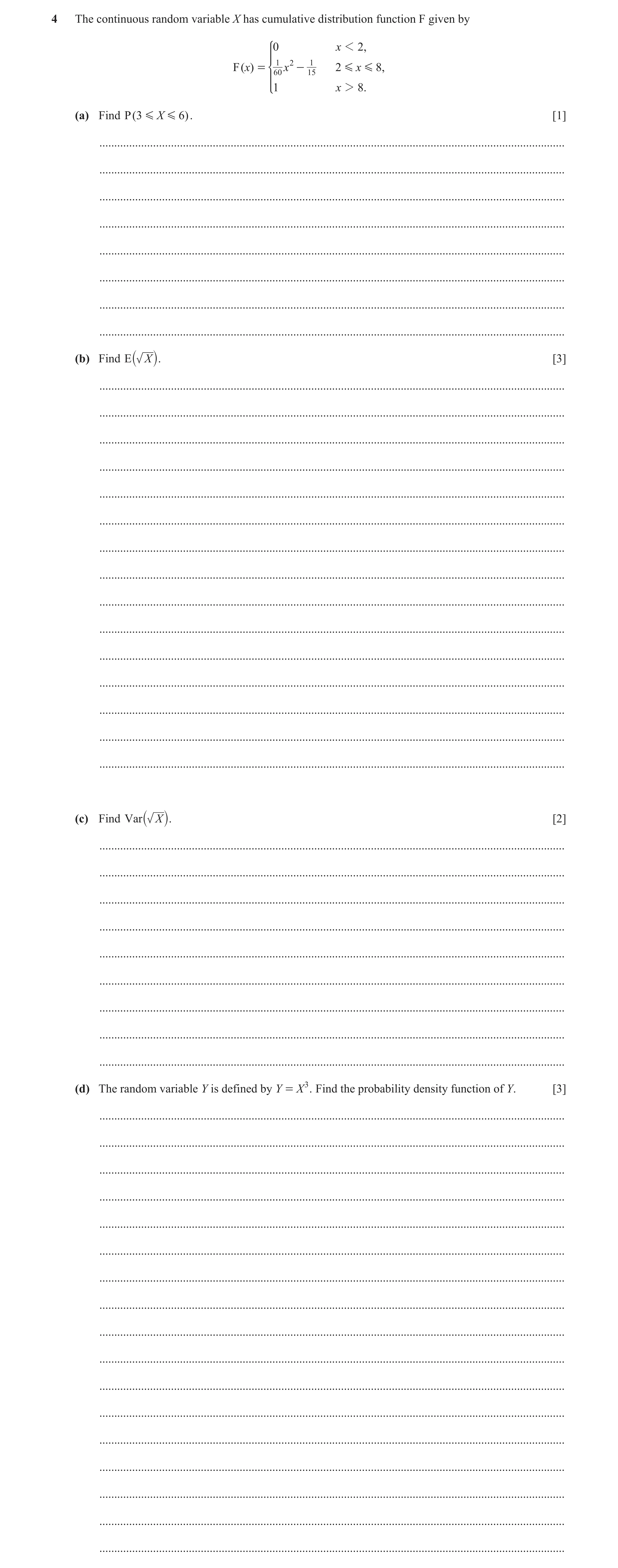
4 The continuous random variable X has cumulative distribution function F given by 0 x 1 2 , - F ( x) = 601 x 2 1 15 2 G x G 8 , *1 x 2 8 . (a) Find P ( 3 G X G 6). [1] … … … … … … … … (b) Find X . [3] E` j … … … … … … … … … … … … … … … (c) Find X . [2] Var` j … … … … … … … … … (d) The random variable Y is defined by Y = X3 . Find the probability density function of Y. [3] … … … … … … … … … … … … … … … … …
9 marks
Mark scheme: 4(a) F(6) – F(3) = 9 20 or 0.45 B1 1 4(b) ( ) 1 , 2 8 f 30 0, x x x otherwise ≤ ≤ = B1 May be implied. Only need to see ( ) 1 f 30 x x = E( X ) = 8 3 5 2 2 2 1 1 d 30 75 x x x = M1 Integrated = 2.34 A1 2.338… Answer of 2.34 without 5 2 1 75 x scores B1B1 (2/3) 3 4(c) Var( X ) =[ ( ) 8 2 2 3 2 1 1 d ] 30 90 x x x E X = − ( ) ( ) 8 8 2 2 3 2 2 1 1 Var 30 90 X x dx x E X = = − M1 = 5.6 – 2.3382 = 0.133 or 0.134 A1 2 Question Answer Marks Guidance 4(d) G(y) = 2 3 1 1 60 15 y − M1 CDF for Y g(y) = 1 3 1 90 y − for 8 512 y ≤ ≤ (0 otherwise) M1 A1 Differentiate to find PDF for Y Correct g(y) and correct range seen anywhere 3
This question in 9231/42 Oct/Nov 2020
Q6 · The continuous random variable X has cumulative distribution function F given by 0 x 1 0… 9231/43 Oct/Nov 2020
6 The continuous random variable X has cumulative distribution function F given by 0 x 1 0, - x ) 0 G x G 6, F ( x) = 601 ( 16 x 2 *1 x 2 6. (a) Find the interquartile range of X. [4] … … … … … … … … … … … … … (b) Find E ( X 3 ) . [4] … … … … … … … … … … … … … … … … … The random variable Y is such that Y = X . (c) Find the probability density function of Y. [3] … … … … … … … … … … … … … … … … … … … Additional Page If you use the following lined page to complete the answer(s) to any question(s), the question number(s) must be clearly shown. … … … … … … … … … … … … … … … … … … … … … …
11 marks
Mark scheme: 6(a) UQ: F(U) = 0.75: 2 16 45 0 u u − + = M1 Obtain quadratic equation for u or l 8 19 u = − (= 3.64) A1 Value of UQ LQ: 2 16 15 0 l l − + = , 1 l = A1 Value of LQ IQR = UQ – LQ = 7 19 2.64 − = A1 FT 4 6(b) ( ) ( ) 1 8 , f 30 0, x x − = 0 ⩽ x ⩽ 6 otherwise B1 May be implied, only need to see ( ) ( ) 1 f 8 30 x x = − Find E(X3) by integration: ( ) 6 3 4 0 1 8 d 30 x x x − = 6 4 5 0 1 2 5 x x − M1 A1 Attempt integration (with PDF not CDF) limits not required Correct integrated expression, with limits = 34.56 A1 4 6(c) ( ) ( ) 2 4 1 16 60 G y y y = − M1 CDF for Y ( ) ( ) 3 1 32 4 for 0 6 60 g y y y y = − ≤ ≤ M1A1 Differentiate to find PDF for Y Correct g(y) and correct range seen anywhere 3
This question in 9231/43 Oct/Nov 2020
Q7 · The continuous random variable X has cumulative distribution function F given by 0 x 1 0… 9231/41 May/June 2021
3 The continuous random variable X has cumulative distribution function F given by 0 x 1 0, G x G 9, F ( x) = 811 x 2 0 * 1 x 2 9. (a) Find X . [3] E` j … … … … … … … … … … … … (b) Find Var X . [2] ` j … … … … … … … … … … … (c) The random variable Y is given by Y 3 = X . Find the probability density function of Y. [3] … … … … … … … … … … … … … … … … … … … … … … … … … … …
8 marks
Mark scheme: 3(a) 9 1.5 0 2 81 x dx B1 ( ) 2 f , 81 x x = correct expression as integrand. 2.5 2 2 81 5 x × M1 Integrate, FT only on their PDF expression. 12 2.4 5 = A1 3 3(b) ( ) 9 2 2 0 2 d 81 x x their a − M1 3 2 2 9 6 2.4 81 3 25 × − = A1 2 3(c) G(y) = 6 1 81 y M1 g(y) = 5 2 27 y M1 Fully correct including ‘for 3 0 9 y and 0 otherwise’ A1 Condone 2.08 3
This question in 9231/41 May/June 2021
Q8 · The continuous random variable X has cumulative distribution function F given by 0 x 1 0… 9231/42 May/June 2021
3 The continuous random variable X has cumulative distribution function F given by 0 x 1 0, G x G 9, F ( x) = 811 x 2 0 * 1 x 2 9. (a) Find X . [3] E` j … … … … … … … … … … … … (b) Find Var X . [2] ` j … … … … … … … … … … … (c) The random variable Y is given by Y 3 = X . Find the probability density function of Y. [3] … … … … … … … … … … … … … … … … … … … … … … … … … … …
8 marks
Mark scheme: 3(a) 9 1.5 0 2 81 x dx B1 ( ) 2 f , 81 x x = correct expression as integrand. 2.5 2 2 81 5 x × M1 Integrate, FT only on their PDF expression. 12 2.4 5 = A1 3 3(b) ( ) 9 2 2 0 2 d 81 x x their a − M1 3 2 2 9 6 2.4 81 3 25 × − = A1 2 3(c) G(y) = 6 1 81 y M1 g(y) = 5 2 27 y M1 Fully correct including ‘for 3 0 9 y and 0 otherwise’ A1 Condone 2.08 3
This question in 9231/42 May/June 2021
Q9 · The continuous random variable X has probability density function f given by 1 8 0 G x 1… 9231/43 May/June 2021
6 The continuous random variable X has probability density function f given by 1 8 0 G x 1 1, f ()x = 1 (8 - x) 1 G x G 8, 28 *0 otherwise. (a) Find the cumulative distribution function of X. [3] … … … … … … … … … … (b) Find the value of the constant a such that P ( X G a) = 57 . [3] … … … … … … … … … … … … The random variable Y is given by Y = 3 X . (c) Find the probability density function of Y. [5] … … … … … … … … … … … … … … … … … … … … … … … … … … Additional Page If you use the following lined page to complete the answer(s) to any question(s), the question number(s) must be clearly shown. … … … … … … … … … … … … … … … … … … … … … …
11 marks
Mark scheme: 6(a) 2 1 0 1, 8 F( ) 1 1 1 8 1 8. 28 2 7 x x x x x x < = − − A1 no constant term. Both parts correct, with domains. Any equivalent form, for example: 2 2 1 1 7 56 7 x x − − . F(x)= 0 for x < 0 and F(x) = 1 for x > 8. A1 Alternative method for question 6(a) ( ) 2 1 0 1, 8 F( ) 1 1 8 1 8. 56 x x x x x < = − − M1 A1 Integrate both parts (all powers of x increase by 1), allow M1 if no constant term. Both parts correct, with domains. Any equivalent form, for example: ( ) 2 1 16 8 56 x x − − . F(x)= 0 for x < 0 and F(x) = 1 for x > 8. A1 3 6(b) F(a) = 5 7 leading to 2 1 1 1 5 8 28 2 7 7 a a − − = *M1 Correct method and attempt to simplify, ft their part (a). 2 16 48 0 a a − + = [ ] 4 12 a a = = DM1 Obtain quadratic and solve. a = 4 A1 Correct single answer, WWW. 3 Question Answer Marks Guidance 6(c) ( ) 3 6 3 1 8 G 1 0 1, 1 16 1 2 ( 56 7 ) . y y y y y y = < − − M1 A1 Substitute x = y3 into both parts of their F(x) from part (a). Correct functions in terms of y, any equivalent form. 0 y < 1 and 1 y 2seen in CDF or PDF A1 Condone instead of <. ( ) 2 2 5 3 0 1, 8 3 g( ) 8 1 2, 28 0 otherwise. y y y y y y < = − < M1 A1 Differentiate their G(y), all powers of y decrease by 1. Must include ‘otherwise’. 5 Question Answer Marks Guidance 6(c) Alternative method for question 6(c) 1 2 2 3 3 1 , d d , d 3 d 3 y x y x x x y y − = = = M1 ( ) 2 1 3 0 1, f d d d 8 8 x x x x y y < = = M1 ( ) 2 3 g 8 y y = A1 ( ) ( ) ( ) 3 2 1 1 1 8, f d 8 d 8 3 d 28 28 x x x x x y y y = − = − ( ) ( ) 2 5 3 8 28 g y y y = − A1 0 y < 1 and 1 y 2 seen in CDF or PDF A1 5
This question in 9231/43 May/June 2021
Q10 · The continuous random variable X has cumulative distribution function F given by Z ] 0 x… 9231/41 Oct/Nov 2021
2 The continuous random variable X has cumulative distribution function F given by Z ] 0 x 1 - 1, ]] 1 2 2 ( 1 + x) - 1 G x G 0 , F ( x) = [ 1 2 1 - 2 ( 1 - x) 0 1 x G 1, ] ] 1 x 2 1. \ (a) Find the probability density function of X. [2] … … … … … … … … … … … (b) Find P - 12 1 G X G 2 [2] b l. … … … … … … … … … … … (c) Find E ( X 2 ) . [2] … … … … … … … … … … … … … (d) Find Var ( X 2 ) . [2] … … … … … … … … … … … … …
8 marks
Mark scheme: 2(a) , f ( ) otherwise. 1 1 0 1 1 0 ì + - ïïïï = - < íïïïïî x x x x x ≤ ≤ 0 ≤, M1 Differentiation attempted. A1 All correct, including 0 otherwise. 2 2(b) P 1 1 2 2 X − = 1 1 7 1 F F 2 2 8 8 − − = − M1 Can do by integration with correct limits. 3 4 A1 2 2(c) ( ) ( ) 0 1 2 2 1 0 1 1 x x dx x x dx − + + − 3 4 3 4 1 1 1 1 3 4 3 4 x x x x + + − M1 1 1 1 12 12 6 + = A1 2 Question Answer Marks Guidance 2(d) ( ) ( ) 0 1 2 4 4 1 0 1 1 1 6 x x dx x x dx − + + − − 5 6 5 6 1 1 1 1 1 5 6 5 6 36 x x x x + + − − M1 Complete method with their mean squared explicit. 1 1 7 15 36 180 − = A1 2
This question in 9231/41 Oct/Nov 2021
Q11 · The continuous random variable X has probability density function f given by a + 15 x 0 G… 9231/42 Oct/Nov 2021
3 The continuous random variable X has probability density function f given by a + 15 x 0 G x 1 1 , G x G 2 , f ( x) = 2a - 15 x 1 * 0 otherwise, where a is a constant. (a) Find the value of a. [3] … … … … … … … … … … … (b) Find E ( X 2 ) . [2] … … … … … … … … … … … … … … … … … … (c) Find the cumulative distribution function of X. [3] … … … … … … … … … … … … … … … … … … … …
8 marks
Mark scheme: 3(a) Total prob = 1, so 1 2 0 1 1 1 2 1 5 5 + + − = a x dx a x dx 2 2 1 1 2 10 10 + + − ax x ax x = 1 *M1 Correct expression integrated and equated to 1. Powers of x correct. 1 3 1 5 − = a DM1 Limits used and attempt to solve. Solve to give 2 5 = a A1 3 3(b) ( ) ( ) 1 2 2 2 0 1 1 1 2 4 5 5 + + − x x dx x x dx 3 4 3 4 1 2 1 1 4 1 5 3 4 5 3 4 + + − x x x x M1 Correct expressions integrated, FT their a. 13 10 A1 11 67 60 60 + 2 Question Answer Marks Guidance 3(c) 2 2 0 < 0 1 1 2 + 0 <1, 5 2 F( ) = 1 1 4 1 1 2, 5 2 1 > 2. x x x x x x x x x ìïïïï æ ö ï ÷ ç ï ÷ ç ï ÷ çè ø ïïíï æ ö ï ÷ ç ï ÷ ç ÷ ï çè ø ï - ï - ïï ïî M1 Integration of their PDF. A1 Middle 2 parts correct. ( ) 0 0 and 1 ( 2) x x = < = > A1 First and last parts correct and all domains correct, with no gaps. 3
This question in 9231/42 Oct/Nov 2021
Q12 · The continuous random variable X has cumulative distribution function F given by Z ] 0 x… 9231/43 Oct/Nov 2021
2 The continuous random variable X has cumulative distribution function F given by Z ] 0 x 1 - 1, ]] 1 2 2 ( 1 + x) - 1 G x G 0 , F ( x) = [ 1 2 1 - 2 ( 1 - x) 0 1 x G 1, ] ] 1 x 2 1. \ (a) Find the probability density function of X. [2] … … … … … … … … … … … (b) Find P - 12 1 G X G 2 [2] b l. … … … … … … … … … … … (c) Find E ( X 2 ) . [2] … … … … … … … … … … … … … (d) Find Var ( X 2 ) . [2] … … … … … … … … … … … … …
8 marks
Mark scheme: 2(a) , f ( ) otherwise. 1 1 0 1 1 0 ì + - ïïïï = - < íïïïïî x x x x x ≤ ≤ 0 ≤, M1 Differentiation attempted. A1 All correct, including 0 otherwise. 2 2(b) P 1 1 2 2 X − = 1 1 7 1 F F 2 2 8 8 − − = − M1 Can do by integration with correct limits. 3 4 A1 2 2(c) ( ) ( ) 0 1 2 2 1 0 1 1 x x dx x x dx − + + − 3 4 3 4 1 1 1 1 3 4 3 4 x x x x + + − M1 1 1 1 12 12 6 + = A1 2 Question Answer Marks Guidance 2(d) ( ) ( ) 0 1 2 4 4 1 0 1 1 1 6 x x dx x x dx − + + − − 5 6 5 6 1 1 1 1 1 5 6 5 6 36 x x x x + + − − M1 Complete method with their mean squared explicit. 1 1 7 15 36 180 − = A1 2
This question in 9231/43 Oct/Nov 2021
Q13 · The continuous random variable X has probability density function f given by kx ( 4 - x)… 9231/41 May/June 2022
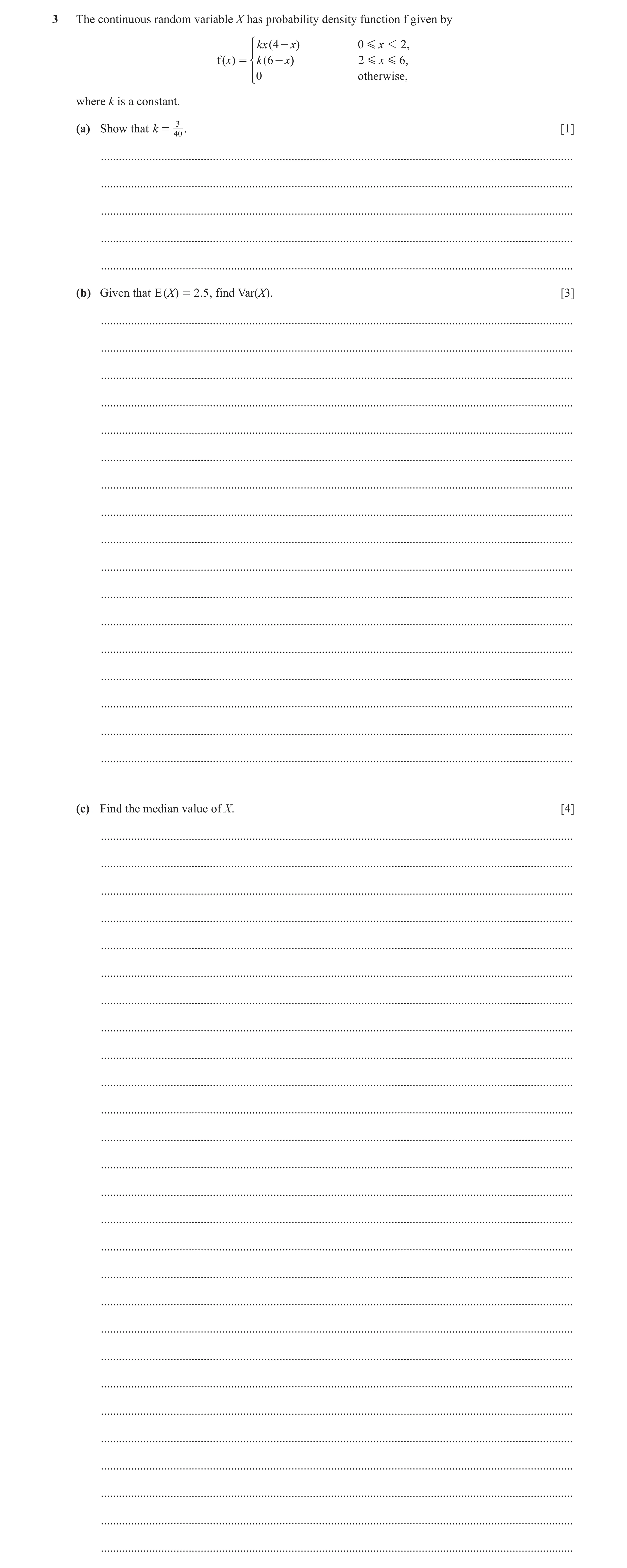
3 The continuous random variable X has probability density function f given by kx ( 4 - x) 0 G x 1 2, f ( x) = k ( 6- x) 2 G x G 6 , * 0 otherwise, where k is a constant. (a) Show that k = 403 . [1] … … … … … (b) Given that E ( X ) = 2.5 , find Var(X). [3] … … … … … … … … … … … … … … … … … (c) Find the median value of X. [4] … … … … … … … … … … … … … … … … … … … … … … … … … … …
8 marks
Mark scheme: 3(a) 2 3 2 1 1 2 6 1 3 2 k x x k x x 8 40 8 36 18 12 2 1 3 3 k k 3 40 k 1 3(b) E(X 2) = 2 6 3 4 2 3 0 2 4 6 d k x x dx k x x x = 4 5 3 4 1 1 2 5 4 k x x k x x = 9.6 96 7.92 k M1* Attempt at E(X 2), correct limits, integrated. Var(X) = E(X2) – E2(X) = 2 (7.92) 2.5 their depM1 Use of correct formula, with their E(X2). 1.67 A1 3 Question Answer Marks Guidance 3(c) 2 0 2 1 4 6 2 m kx x dx k x M1* Correct expression and attempt to integrate. 2 0 2 4 5 kx x dx B1 May be implied 2 2 1 1 6 5 2 2 k x x 2 1 1 6 12 2 2 10 m m k 2 68 12 0 3 m m depM1 First integral and 1 2 may be seen combined as 1 10 . Obtain quadratic equation. 2 6 30 3 m 2 6 30 2.35 3 m A1 Single answer. 4
This question in 9231/41 May/June 2022
Q14 · A scientist is investigating the numbers of a particular type of butterfly in a certain… 9231/41 May/June 2022
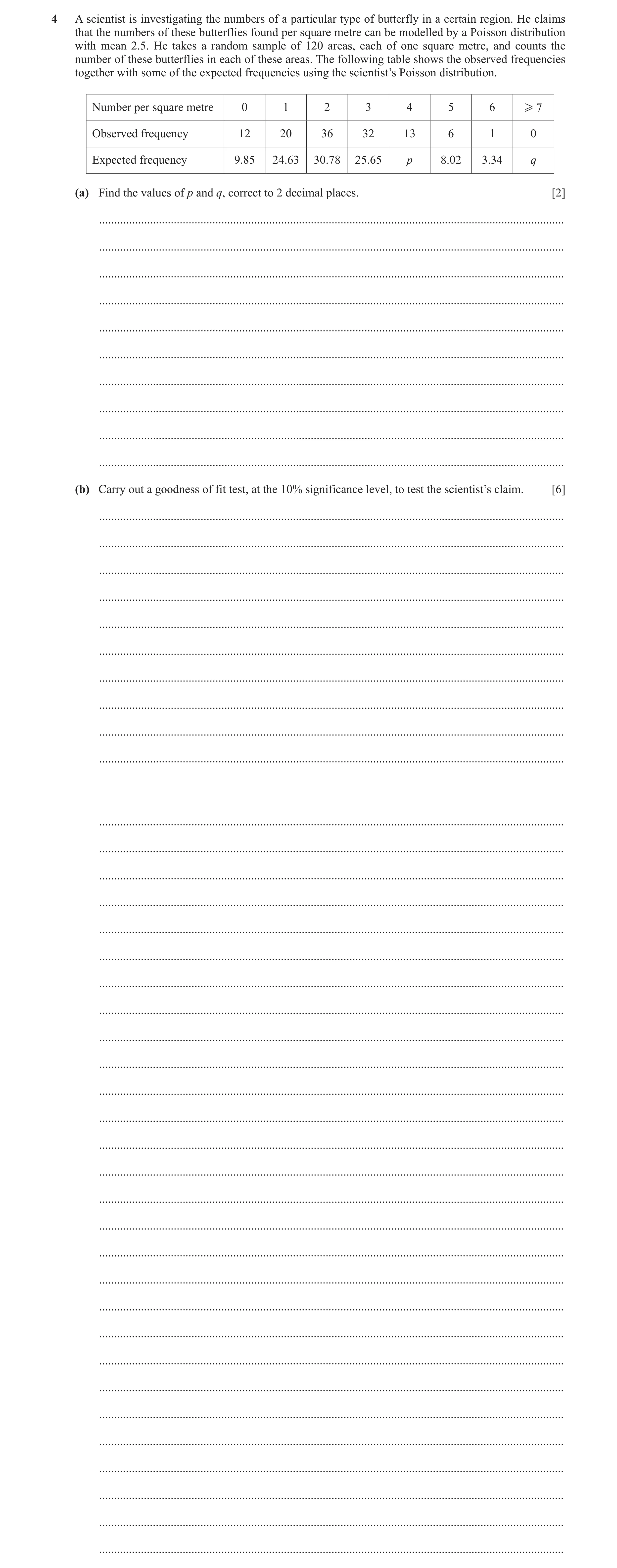
4 A scientist is investigating the numbers of a particular type of butterfly in a certain region. He claims that the numbers of these butterflies found per square metre can be modelled by a Poisson distribution with mean 2.5. He takes a random sample of 120 areas, each of one square metre, and counts the number of these butterflies in each of these areas. The following table shows the observed frequencies together with some of the expected frequencies using the scientist’s Poisson distribution. Number per square metre 0 1 2 3 4 5 6 H 7 Observed frequency 12 20 36 32 13 6 1 0 Expected frequency 9.85 24.63 30.78 25.65 p 8.02 3.34 q (a) Find the values of p and q, correct to 2 decimal places. [2] … … … … … … … … … … (b) Carry out a goodness of fit test, at the 10% significance level, to test the scientist’s claim. [6] … … … … … … … … … … … … … … … … … … … … … … … … … … … … … … … … … … … … … …
8 marks
Mark scheme: 4(a) 1.70 q B1 Condone 1.7 2 Question Answer Marks Guidance 4(b) 0 1 2 3 4 5 6 7 12 20 36 32 13 6 1 0 9.85 24.63 30.78 25.65 16.03 8.02 3.34 1.70 Combine last two columns: O value = 1, E value = 5.04 M1 Add last 2 columns (or 3 columns: 13.06). Calculate values of 2 O E E : 0.4693 0.8704 0.8853 1.5720 0.5727 0.5088 3.2384 M1 Calculate values. Test statistic = 8.12 A1 H0: data fits a Poisson distribution with mean 2.5 H1: data does not fit a Poisson distribution with mean 2.5 B1 Need data and distribution. e.g Data fits the given distribution. Number of butterflies per square metre fits Po(2.5). Critical value of chi-squared = 10.64 Compare: ‘8.12’ < 10.64, accept H0 M1 Compare their test statistic with 10.64. Note: allow 9.236 if 3 columns combined or 12.02 if none combined. There is sufficient evidence to support the scientist’s claim / there is sufficient evidence to suggest that the data fits a Poisson distribution with mean 2.5 A1 Correct conclusion, in context. Level of uncertainty in language is used. 6
This question in 9231/41 May/June 2022
Q15 · The continuous random variable X has probability density function f given by kx ( 4 - x)… 9231/42 May/June 2022
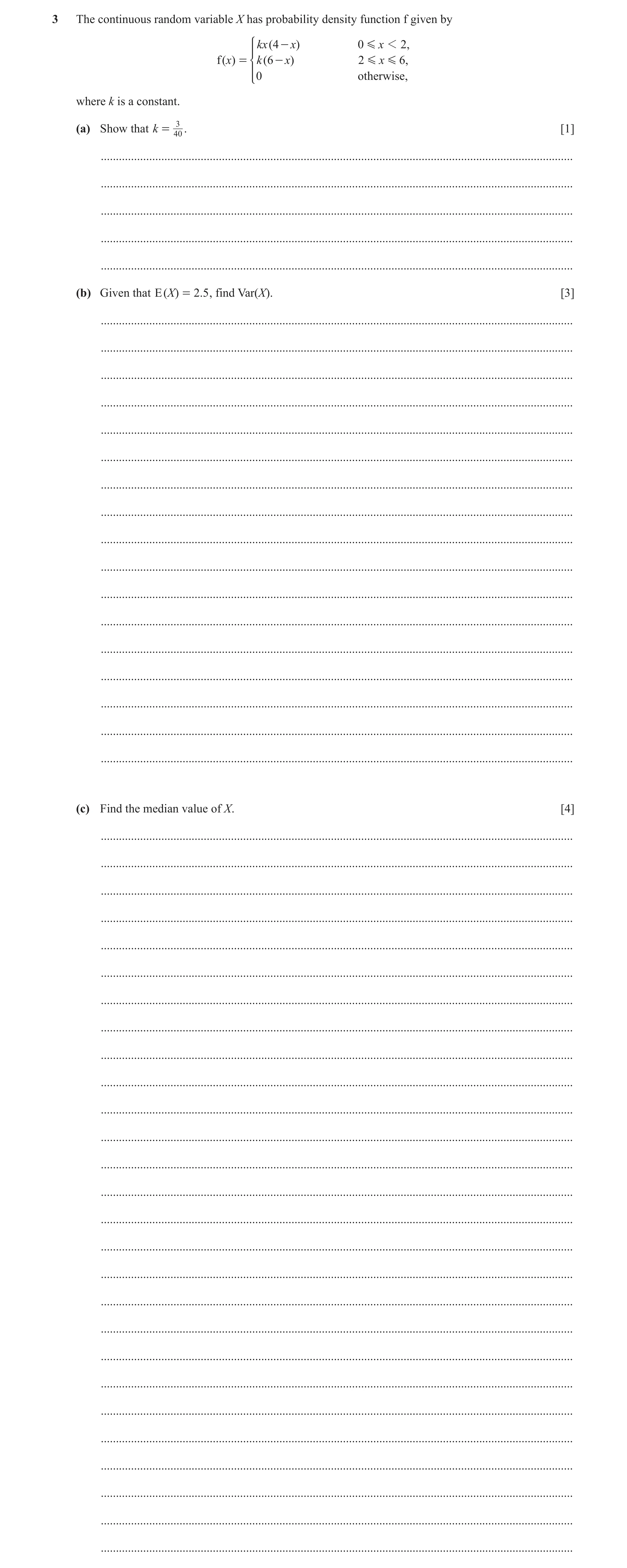
3 The continuous random variable X has probability density function f given by kx ( 4 - x) 0 G x 1 2, f ( x) = k ( 6- x) 2 G x G 6 , * 0 otherwise, where k is a constant. (a) Show that k = 403 . [1] … … … … … (b) Given that E ( X ) = 2.5 , find Var(X). [3] … … … … … … … … … … … … … … … … … (c) Find the median value of X. [4] … … … … … … … … … … … … … … … … … … … … … … … … … … …
8 marks
Mark scheme: 3(a) 2 3 2 1 1 2 6 1 3 2 k x x k x x 8 40 8 36 18 12 2 1 3 3 k k 3 40 k 1 3(b) E(X 2) = 2 6 3 4 2 3 0 2 4 6 d k x x dx k x x x = 4 5 3 4 1 1 2 5 4 k x x k x x = 9.6 96 7.92 k M1* Attempt at E(X 2), correct limits, integrated. Var(X) = E(X2) – E2(X) = 2 (7.92) 2.5 their depM1 Use of correct formula, with their E(X2). 1.67 A1 3 Question Answer Marks Guidance 3(c) 2 0 2 1 4 6 2 m kx x dx k x M1* Correct expression and attempt to integrate. 2 0 2 4 5 kx x dx B1 May be implied 2 2 1 1 6 5 2 2 k x x 2 1 1 6 12 2 2 10 m m k 2 68 12 0 3 m m depM1 First integral and 1 2 may be seen combined as 1 10 . Obtain quadratic equation. 2 6 30 3 m 2 6 30 2.35 3 m A1 Single answer. 4
This question in 9231/42 May/June 2022
Q16 · A scientist is investigating the numbers of a particular type of butterfly in a certain… 9231/42 May/June 2022
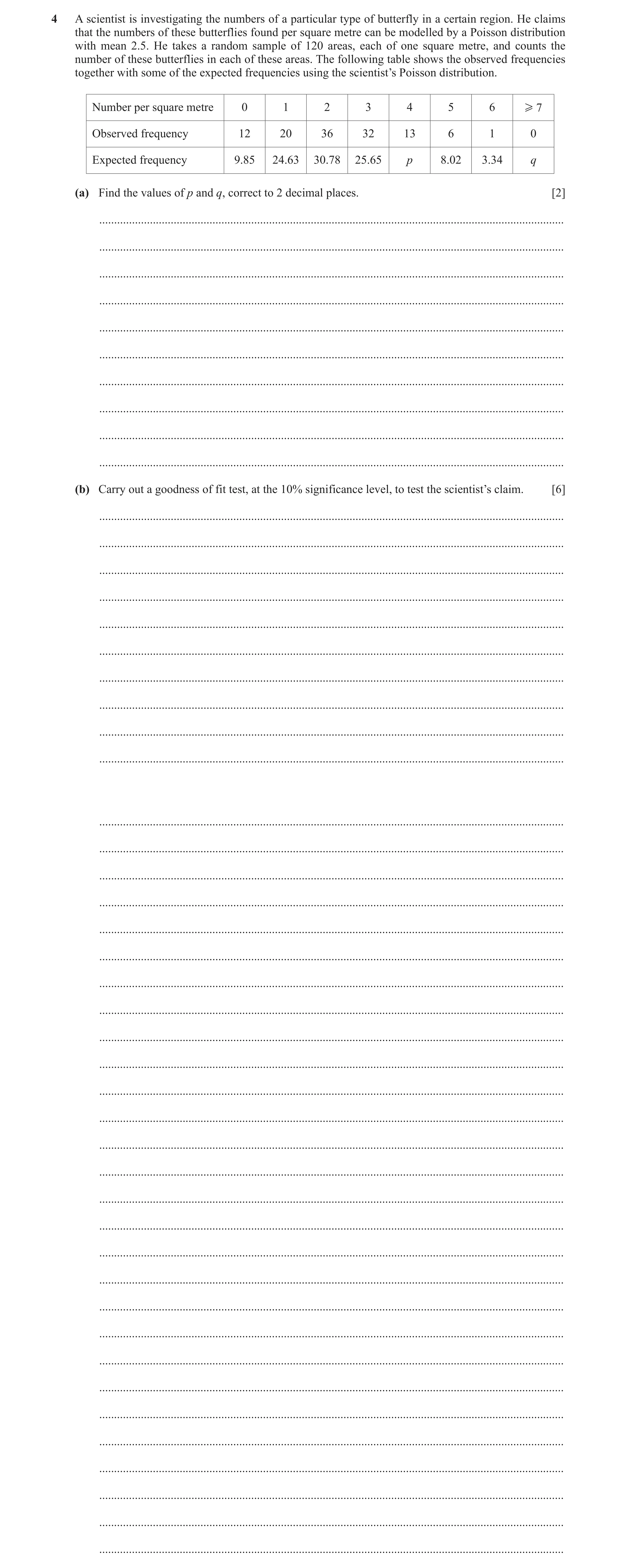
4 A scientist is investigating the numbers of a particular type of butterfly in a certain region. He claims that the numbers of these butterflies found per square metre can be modelled by a Poisson distribution with mean 2.5. He takes a random sample of 120 areas, each of one square metre, and counts the number of these butterflies in each of these areas. The following table shows the observed frequencies together with some of the expected frequencies using the scientist’s Poisson distribution. Number per square metre 0 1 2 3 4 5 6 H 7 Observed frequency 12 20 36 32 13 6 1 0 Expected frequency 9.85 24.63 30.78 25.65 p 8.02 3.34 q (a) Find the values of p and q, correct to 2 decimal places. [2] … … … … … … … … … … (b) Carry out a goodness of fit test, at the 10% significance level, to test the scientist’s claim. [6] … … … … … … … … … … … … … … … … … … … … … … … … … … … … … … … … … … … … … …
8 marks
Mark scheme: 4(a) 1.70 q B1 Condone 1.7 2 Question Answer Marks Guidance 4(b) 0 1 2 3 4 5 6 7 12 20 36 32 13 6 1 0 9.85 24.63 30.78 25.65 16.03 8.02 3.34 1.70 Combine last two columns: O value = 1, E value = 5.04 M1 Add last 2 columns (or 3 columns: 13.06). Calculate values of 2 O E E : 0.4693 0.8704 0.8853 1.5720 0.5727 0.5088 3.2384 M1 Calculate values. Test statistic = 8.12 A1 H0: data fits a Poisson distribution with mean 2.5 H1: data does not fit a Poisson distribution with mean 2.5 B1 Need data and distribution. e.g Data fits the given distribution. Number of butterflies per square metre fits Po(2.5). Critical value of chi-squared = 10.64 Compare: ‘8.12’ < 10.64, accept H0 M1 Compare their test statistic with 10.64. Note: allow 9.236 if 3 columns combined or 12.02 if none combined. There is sufficient evidence to support the scientist’s claim / there is sufficient evidence to suggest that the data fits a Poisson distribution with mean 2.5 A1 Correct conclusion, in context. Level of uncertainty in language is used. 6
This question in 9231/42 May/June 2022
Q17 · The continuous random variable X has probability density function f given by 3 1 1 + 2 1… 9231/43 May/June 2022
4 The continuous random variable X has probability density function f given by 3 1 1 + 2 1 G x G 3, f ( x) = 8 e x o otherwise. * 0 (a) Find X [3] E` j. … … … … … … … … … … … … The random variable Y is given by Y = X 2 . (b) Find the probability density function of Y. [4] … … … … … … … … … … … … … … … … … (c) Find the 40th percentile of Y. [3] … … … … … … … … … … … … … … … … … … … … …
10 marks
Mark scheme: 4(a) E( 3 0.5 1.5 2 1 3 1 3 ) 1 d d 8 8 X x x x x x x 1.5 0.5 3 2 2 8 3 x x A1 3 2 2 1 2 3 2 1 3 8 3 2 3 ( = 1.37) A1 3 Question Answer Marks Guidance 4(b) 3 1 8 F x x x M1 Integrate. 3 1 8 G y y y M1 Change variable throughout in their CDF. 0.5 1.5 3 , 1 9 16 g y y y y A1 Differentiate to find g(y). 0 otherwise A1 1 9 y and 0 otherwise, dependent on second M1. 4 4(c) 0.4 F p so 3 1 0.4 8 p p M1* Correct method. 2 15 16 15 0 p p 5 5 3 3 5 0, 3 p p p M1 dep Obtain quadratic and solve. 40th percentile of Y is 25 9 A1 3
This question in 9231/43 May/June 2022
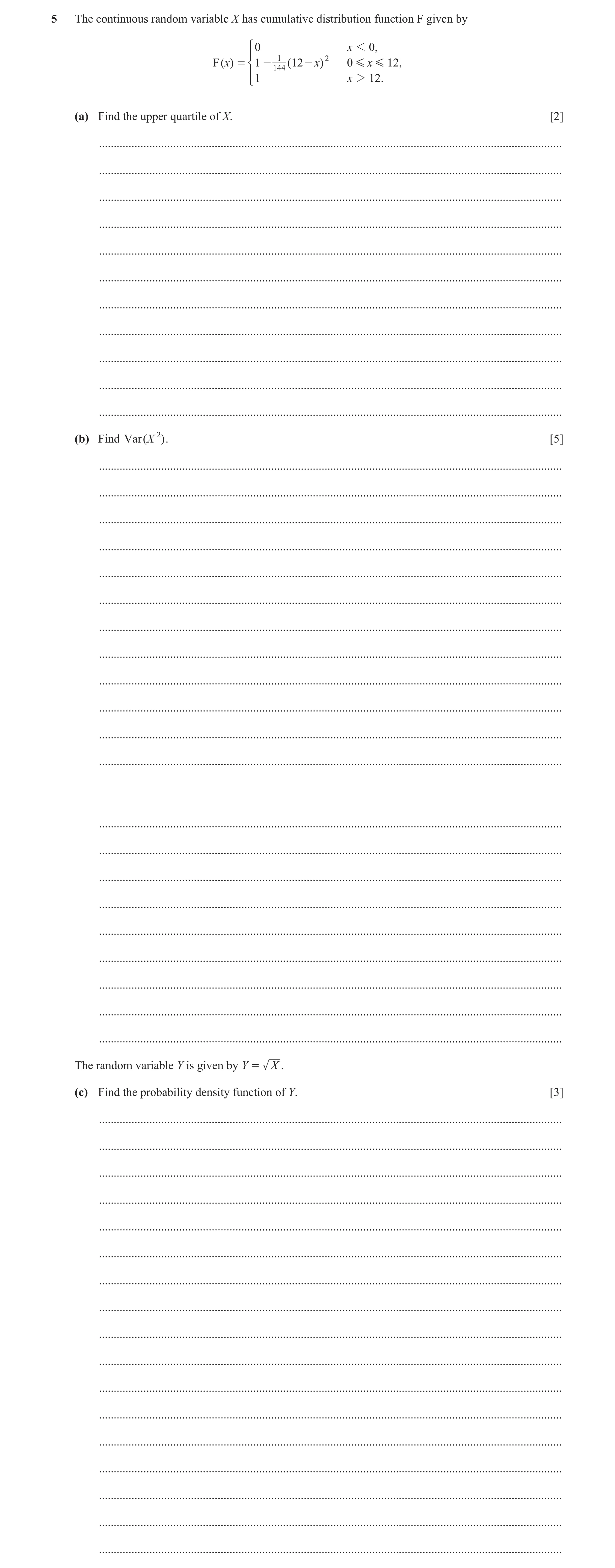
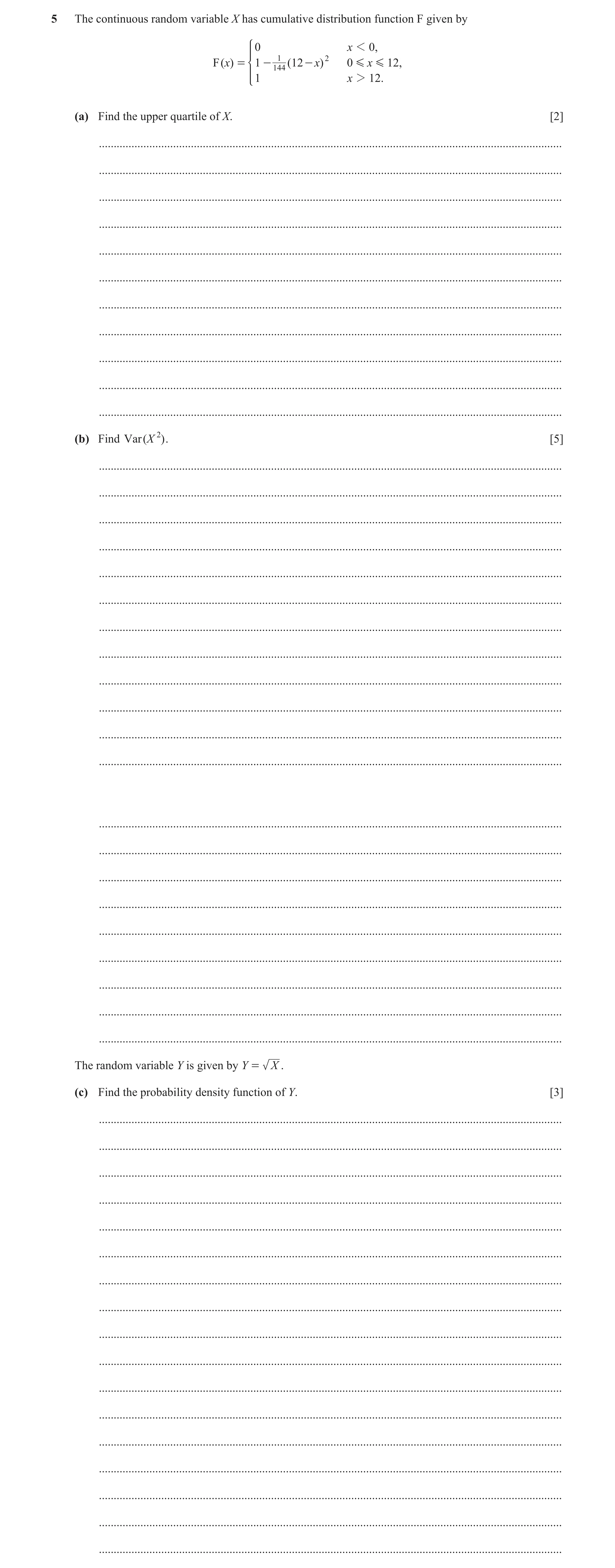
Q18 · The continuous random variable X has cumulative distribution function F given by 0 x 1 0… 9231/41 Oct/Nov 2022
5 The continuous random variable X has cumulative distribution function F given by 0 x 1 0, - x) 0 G x G 12, F ( x) = 1 - 1441 ( 12 2 * 1 x 2 12. (a) Find the upper quartile of X. [2] … … … … … … … … … … … (b) Find V ar (X 2 ) . [5] … … … … … … … … … … … … … … … … … … … … … The random variable Y is given by Y = X . (c) Find the probability density function of Y. [3] … … … … … … … … … … … … … … … … …
10 marks
Mark scheme: 5(a) 1 2 3 M1 F(U) = 0.75, so 1 − (12 − U ) = 144 4 (12 − U ) 2 = 36, 12 − U = 6, A1 U = 6 only 2 5(b) 1 B1 Differentiate given PDF. [f(x) =] (12 −x ) 72 12 1 2 3 1 3 1 4 M1 Integrate x 2 f ( x ) with their f ( x ) . 2 E( X ) = (12 x − x ) dx = 4 x − x [= 24] 0 72 72 4 4 12 1 4 5 1 12 5 1 6 M1 Integrate x 4 f ( x ) with their f ( x ) . E X = 12 x − x dx = x − x [= 1382.4] ( ) ( ) 0 72 72 5 6 Var X 2 = E X 4 − E 2 X 2 [ = 1382.4 − 24 2 ] M1 Using correct formula with numerical values possibly ( ) ( ) ( ) unsimplified. 1382.4 − 576 = 806 (.4 ) A1 5 25(c) 0 y 0, M1 1 2 Change the variable: 1 − 12 −y ( ) 2 144 1 2 12 − y 0 y 12, Allow domain unchanged at this stage. G ( y ) = 1 − ( ) 144 1 y 12. 1 3 M1 Differentiate their G ( y ) . 12 y − y ( ) 36 1 3 A1 Fully correct. 12 y − y 0 y 12 ( ) g ( y ) = 36 0 otherwise
This question in 9231/41 Oct/Nov 2022
Q19 · The continuous random variable X has probability density function f given by k 0 G x 1 1… 9231/42 Oct/Nov 2022
4 The continuous random variable X has probability density function f given by k 0 G x 1 1, f ( x) = kx 1 G x G 2, * 0 otherwise, where k is a constant. (a) Show that k = 25 . [1] … … … … … … … (b) Find the interquartile range of X. [5] … … … … … … … … … … … … … … … (c) Find Var ( X) . [4] … … … … … … … … … … … … … … … … … … … … … … … … … … …
10 marks
Mark scheme: 4(a) 1 2 B1 Integration and k + 3k/2 = 1 oe seen. k 2 3 2 x , k + k = 1, k = kxdx = kx + kdx + 2 5 2 0 1 1 4(b) kx 0 x 1, M1 CDF or integration with 1 x 2 + 1 seen. F ( x ) = k 2 1 5 5 x + 1 x 2 2 5 k 2 1 M1 Method for UQ UQ: x + = 3, 2 5 4 2 3 2 11 1 A1 UQ x + 1 = 5 , x = x = 11 4 4 2 1 5 B1 LQ LQ: kx = , x = 4 8 1 5 A1 CAO IQR = 11 − = 1.03 ( 3 ) 2 8 5 4(c) 1 2 M1 With correct limits. 2 k 2 k 3 17 E(X) = kxdx + kx dx = x + x = 2 3 15 0 1 1 2 M1 With correct limits. 2 3 k 3 k 4 49 E(X2) = kx dx + kx dx = x + x = 3 4 30 0 1 2 M1 Using correct formula with numerical values. 49 17 Var(X) = − 30 15 157 A1 ( = 0.349 ) 450 4
This question in 9231/42 Oct/Nov 2022
Q20 · The continuous random variable X has cumulative distribution function F given by 0 x 1 0… 9231/43 Oct/Nov 2022
5 The continuous random variable X has cumulative distribution function F given by 0 x 1 0, - x) 0 G x G 12, F ( x) = 1 - 1441 ( 12 2 * 1 x 2 12. (a) Find the upper quartile of X. [2] … … … … … … … … … … … (b) Find V ar (X 2 ) . [5] … … … … … … … … … … … … … … … … … … … … … The random variable Y is given by Y = X . (c) Find the probability density function of Y. [3] … … … … … … … … … … … … … … … … …
10 marks
Mark scheme: 5(a) 1 2 3 M1 F(U) = 0.75, so 1 − (12 − U ) = 144 4 (12 − U ) 2 = 36, 12 − U = 6, A1 U = 6 only 2 5(b) 1 B1 Differentiate given PDF. [f(x) =] (12 −x ) 72 12 1 2 3 1 3 1 4 M1 Integrate x 2 f ( x ) with their f ( x ) . 2 E( X ) = (12 x − x ) dx = 4 x − x [= 24] 0 72 72 4 4 12 1 4 5 1 12 5 1 6 M1 Integrate x 4 f ( x ) with their f ( x ) . E X = 12 x − x dx = x − x [= 1382.4] ( ) ( ) 0 72 72 5 6 Var X 2 = E X 4 − E 2 X 2 [ = 1382.4 − 24 2 ] M1 Using correct formula with numerical values possibly ( ) ( ) ( ) unsimplified. 1382.4 − 576 = 806 (.4 ) A1 5 25(c) 0 y 0, M1 1 2 Change the variable: 1 − 12 −y ( ) 2 144 1 2 12 − y 0 y 12, Allow domain unchanged at this stage. G ( y ) = 1 − ( ) 144 1 y 12. 1 3 M1 Differentiate their G ( y ) . 12 y − y ( ) 36 1 3 A1 Fully correct. 12 y − y 0 y 12 ( ) g ( y ) = 36 0 otherwise
This question in 9231/43 Oct/Nov 2022
Q21 · A random sample of 50 values of the continuous random variable X was taken 9231/41 May/June 2023
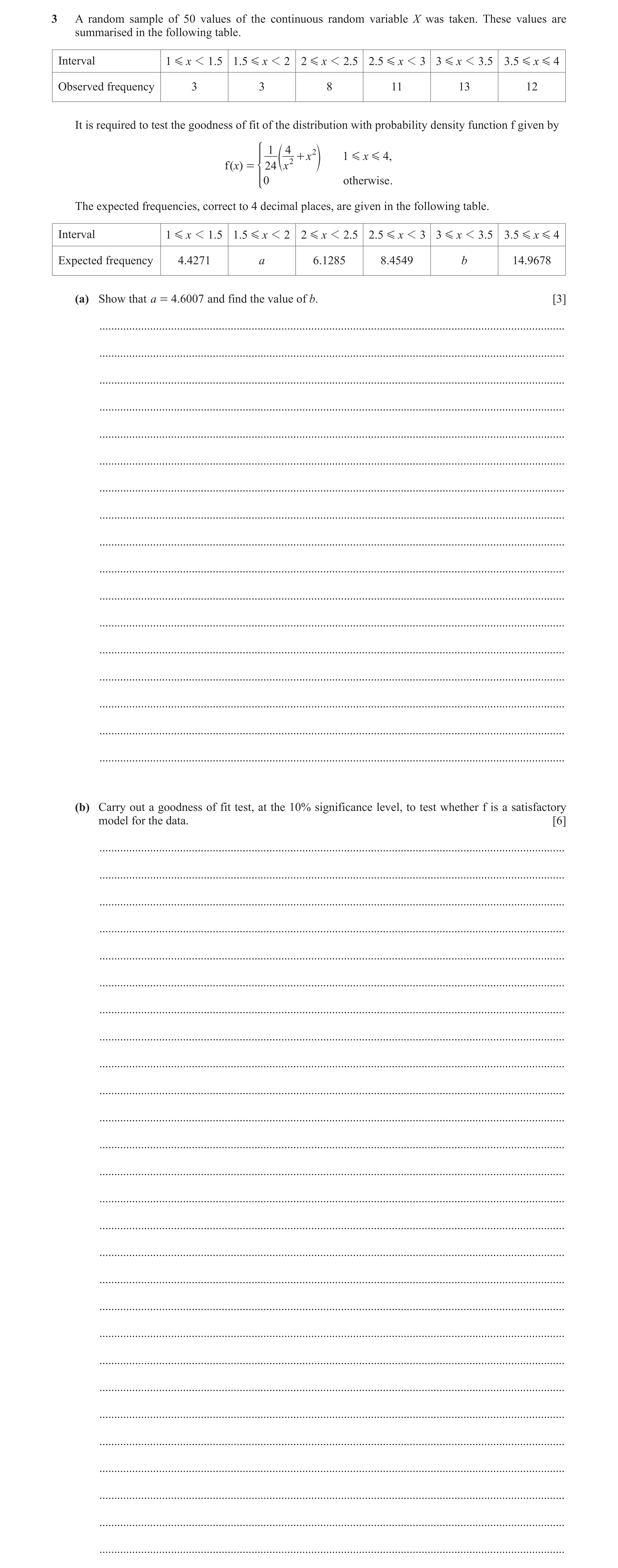
3 A random sample of 50 values of the continuous random variable X was taken. These values are summarised in the following table. Interval 1 G x 1 1 .5 1.5 G x 1 2 2 G x 1 2.5 2.5 G x 1 3 3 G x 1 3.5 3.5 G x G 4 Observed frequency 3 3 8 11 13 12 It is required to test the goodness of fit of the distribution with probability density function f given by 1 4 2 + x 1 G x G 4, 2 f ( x) = * 024e x o otherwise . The expected frequencies, correct to 4 decimal places, are given in the following table. Interval 1 G x 1 1.5 1.5 G x 1 2 2 G x 1 2.5 2.5 G x 1 3 3 G x 1 3.5 3.5 G x G 4 Expected frequency 4.4271 a 6.1285 8.4549 b 14.9678 (a) Show that a = 4.6007 and find the value of b. [3] … … … … … … … … … … … … … … … … … (b) Carry out a goodness of fit test, at the 10% significance level, to test whether f is a satisfactory model for the data. [6] … … … … … … … … … … … … … … … … … … … … … … … … … … …
9 marks
Mark scheme: 3(a) 3 2 2 2 1.5 1 4 1 4 d 24 24 3 x x x x x M1 Integration with correct powers and correct limits seen. 50 a 0.092014 = 4.6007 A1 AG 53 576 or 1325 288 or 0.092014 or 4.60069 seen 11.4211 b B1 Or 11.421(0) 3 3(b) Combine first two columns: 6, 9.0278 M1 Must be seen, or implied by 1.0155. Calculate value of chi-squared: 1.0155 + 0.5715 + 0.7661 + 0.2183 + 0.5885 M1 At least 2 correct values (at least 3sf) or expressions seen. Allow columns not combined or three columns combined. 3.16 A1 CWO. Dependent on M1M1 scored. SCB1 for 3.16 with no working H0: f is a good fit for the data H1: f is not a good fit for the data B1 Tabular value of chi-squared: 7.78 ‘3.16’ < 7.78 and accept H0 M1 Correct tabular value: allow correct FT value if columns not combined (9.236) or three columns combined (6.251). Insufficient evidence to suggest that f is not a good fit for the data Condone: sufficient evidence to suggest that f is a good fit for the data. A1 Correct conclusion in context, following correct work, level of uncertainty in language (not ‘prove’, not ‘there is no evidence’), no contradictions. A0 if hypotheses reversed 6
This question in 9231/41 May/June 2023
Q22 · The continuous random variable X has probability density function f given by 3 2 1 x - 21… 9231/41 May/June 2023
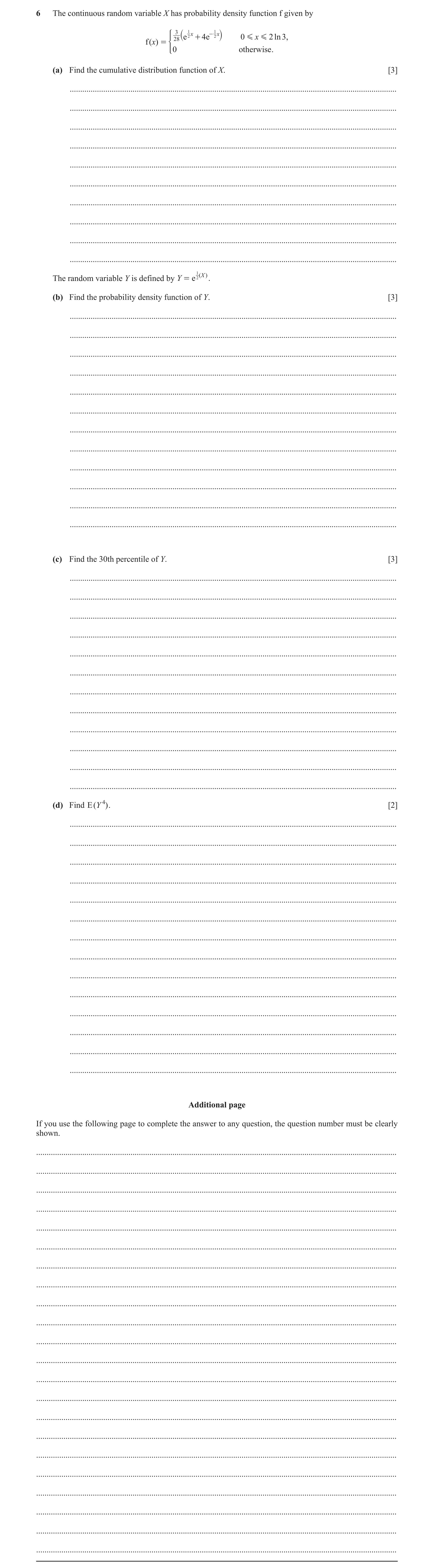
6 The continuous random variable X has probability density function f given by 3 2 1 x - 21 x 28 e + 4 e 0 G x G 2 ln 3 , f ( x) = ` j * 0 otherwise . (a) Find the cumulative distribution function of X. [3] … … … … … … … … … … 2 The random variable Y is defined by Y = e 1 ( X ) . (b) Find the probability density function of Y. [3] … … … … … … … … … … … … (c) Find the 30th percentile of Y. [3] … … … … … … … … … … … … (d) Find E ( Y 4 ) . [2] … … … … … … … … … … … … … … Additional page If you use the following page to complete the answer to any question, the question number must be clearly shown. … … … … … … … … … … … … … … … … … … … … … …
11 marks
Mark scheme: 6(a) F( 1 1 2 2 3 ) 2e 8e 28 x x x c F( 1 1 2 2 3 9 ) 2e 8e 28 14 x x x A1 Correct ranges including 0 2ln3 x associated with their F( ) x F( x ) = 0 for 0 x and 1 for 2ln3 x B1 No gaps in range. 3 6(b) G( 3 8 ) 2 6 28 y y y M1 y substituted into their F. 1 3 y B1 Seen anywhere, condone ln3 1 e y . g( 2 3 8 ) 2 28 y y A1 Correct expression, not containing logs. 3 6(c) 3 8 3 2 6 28 10 y y M1 Their G(y) 3 10 2 5 8 20 0 y y M1 Obtain from G(y) and solve quadratic equation to find y. 1.35 y A1 Single correct answer. 3 Question Answer Marks Guidance 6(d) E(Y 4) = 4 4 2 2 3 3 1 1 3 8 3 2 d 2 8 d 28 28 y y y y y y = 5 3 3 2 8 28 5 3 y y 1 Integrate 4 y their g(y). Limits must be 1 and 3. 17.8 A1 89 5 2
This question in 9231/41 May/June 2023
Q23 · A random sample of 50 values of the continuous random variable X was taken 9231/42 May/June 2023
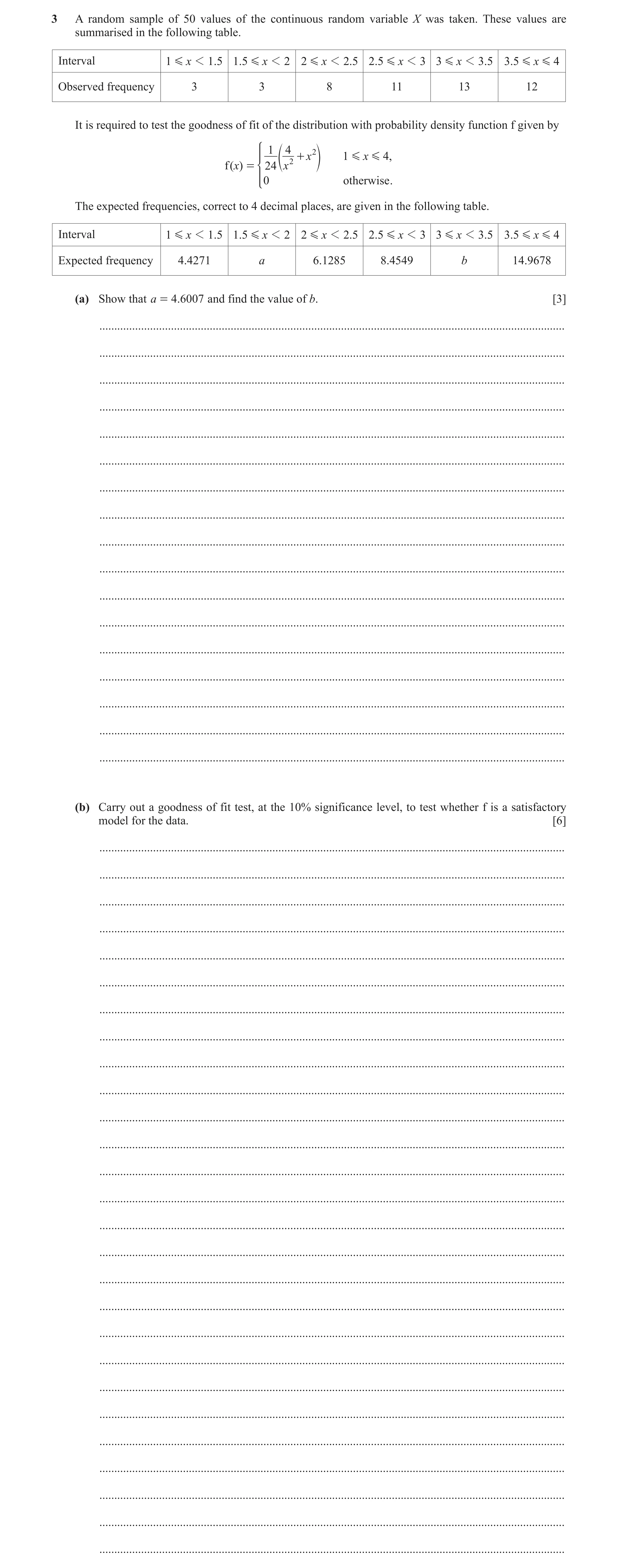
3 A random sample of 50 values of the continuous random variable X was taken. These values are summarised in the following table. Interval 1 G x 1 1 .5 1.5 G x 1 2 2 G x 1 2.5 2.5 G x 1 3 3 G x 1 3.5 3.5 G x G 4 Observed frequency 3 3 8 11 13 12 It is required to test the goodness of fit of the distribution with probability density function f given by 1 4 2 + x 1 G x G 4, 2 f ( x) = * 024e x o otherwise . The expected frequencies, correct to 4 decimal places, are given in the following table. Interval 1 G x 1 1.5 1.5 G x 1 2 2 G x 1 2.5 2.5 G x 1 3 3 G x 1 3.5 3.5 G x G 4 Expected frequency 4.4271 a 6.1285 8.4549 b 14.9678 (a) Show that a = 4.6007 and find the value of b. [3] … … … … … … … … … … … … … … … … … (b) Carry out a goodness of fit test, at the 10% significance level, to test whether f is a satisfactory model for the data. [6] … … … … … … … … … … … … … … … … … … … … … … … … … … …
9 marks
Mark scheme: 3(a) 3 2 2 2 1.5 1 4 1 4 d 24 24 3 x x x x x M1 Integration with correct powers and correct limits seen. 50 a 0.092014 = 4.6007 A1 AG 53 576 or 1325 288 or 0.092014 or 4.60069 seen 11.4211 b B1 Or 11.421(0) 3 3(b) Combine first two columns: 6, 9.0278 M1 Must be seen, or implied by 1.0155. Calculate value of chi-squared: 1.0155 + 0.5715 + 0.7661 + 0.2183 + 0.5885 M1 At least 2 correct values (at least 3sf) or expressions seen. Allow columns not combined or three columns combined. 3.16 A1 CWO. Dependent on M1M1 scored. SCB1 for 3.16 with no working H0: f is a good fit for the data H1: f is not a good fit for the data B1 Tabular value of chi-squared: 7.78 ‘3.16’ < 7.78 and accept H0 M1 Correct tabular value: allow correct FT value if columns not combined (9.236) or three columns combined (6.251). Insufficient evidence to suggest that f is not a good fit for the data Condone: sufficient evidence to suggest that f is a good fit for the data. A1 Correct conclusion in context, following correct work, level of uncertainty in language (not ‘prove’, not ‘there is no evidence’), no contradictions. A0 if hypotheses reversed 6
This question in 9231/42 May/June 2023
Q24 · The continuous random variable X has probability density function f given by 3 2 1 x - 21… 9231/42 May/June 2023
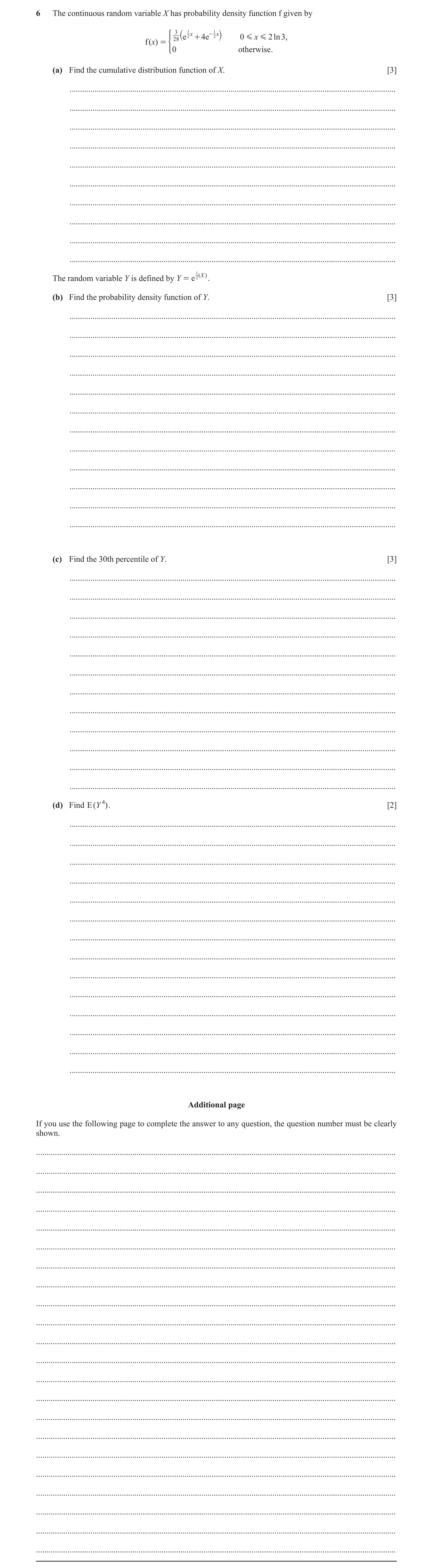
6 The continuous random variable X has probability density function f given by 3 2 1 x - 21 x 28 e + 4 e 0 G x G 2 ln 3 , f ( x) = ` j * 0 otherwise . (a) Find the cumulative distribution function of X. [3] … … … … … … … … … … 2 The random variable Y is defined by Y = e 1 ( X ) . (b) Find the probability density function of Y. [3] … … … … … … … … … … … … (c) Find the 30th percentile of Y. [3] … … … … … … … … … … … … (d) Find E ( Y 4 ) . [2] … … … … … … … … … … … … … … Additional page If you use the following page to complete the answer to any question, the question number must be clearly shown. … … … … … … … … … … … … … … … … … … … … … …
11 marks
Mark scheme: 6(a) F( 1 1 2 2 3 ) 2e 8e 28 x x x c F( 1 1 2 2 3 9 ) 2e 8e 28 14 x x x A1 Correct ranges including 0 2ln3 x associated with their F( ) x F( x ) = 0 for 0 x and 1 for 2ln3 x B1 No gaps in range. 3 6(b) G( 3 8 ) 2 6 28 y y y M1 y substituted into their F. 1 3 y B1 Seen anywhere, condone ln3 1 e y . g( 2 3 8 ) 2 28 y y A1 Correct expression, not containing logs. 3 6(c) 3 8 3 2 6 28 10 y y M1 Their G(y) 3 10 2 5 8 20 0 y y M1 Obtain from G(y) and solve quadratic equation to find y. 1.35 y A1 Single correct answer. 3 Question Answer Marks Guidance 6(d) E(Y 4) = 4 4 2 2 3 3 1 1 3 8 3 2 d 2 8 d 28 28 y y y y y y = 5 3 3 2 8 28 5 3 y y 1 Integrate 4 y their g(y). Limits must be 1 and 3. 17.8 A1 89 5 2
This question in 9231/42 May/June 2023
Q25 · The continuous random variable X has probability density function f given by 1 - 31 - 23… 9231/43 May/June 2023
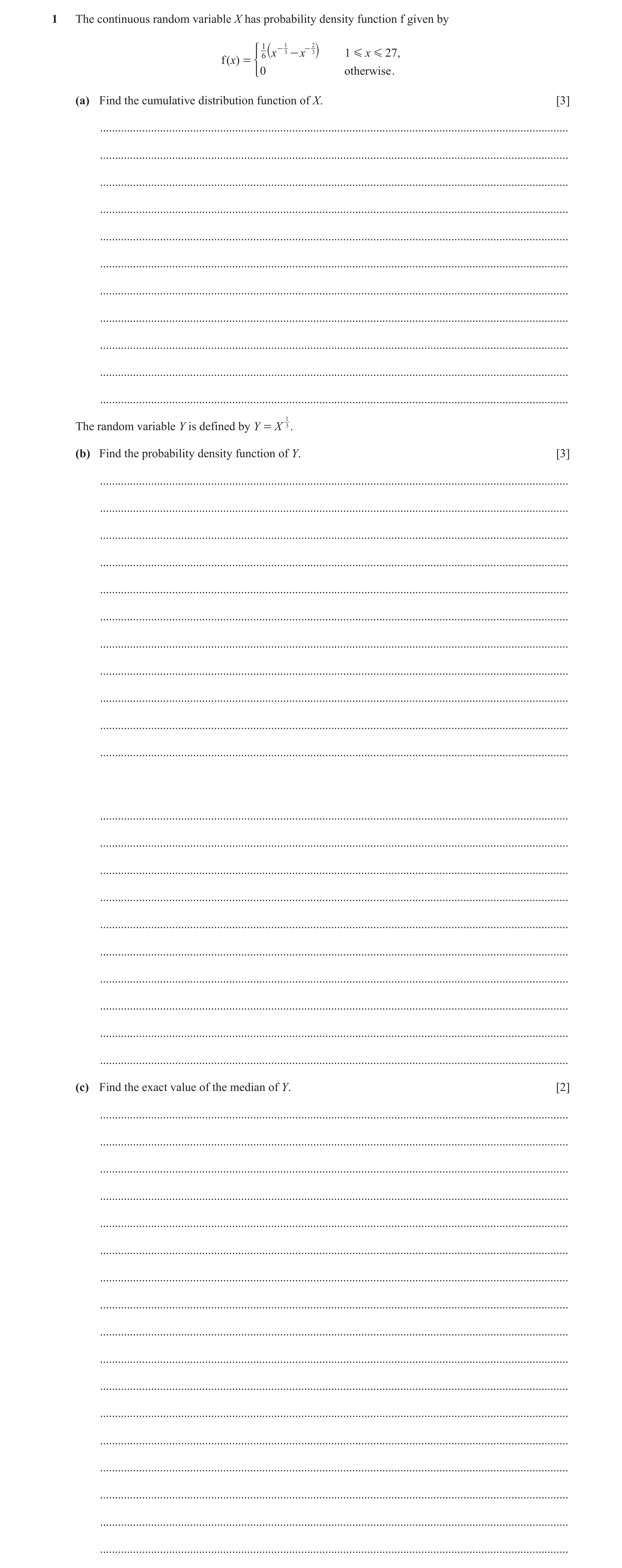
1 The continuous random variable X has probability density function f given by 1 - 31 - 23 6 x - x 1 G x G 27, f ( x) = ` j * 0 otherwise . (a) Find the cumulative distribution function of X. [3] … … … … … … … … … … … 3 . The random variable Y is defined by Y = X 1 (b) Find the probability density function of Y. [3] … … … … … … … … … … … … … … … … … … … … … (c) Find the exact value of the median of Y. [2] … … … … … … … … … … … … … … … … …
8 marks
Mark scheme: 1(a) F( 2 1 3 3 1 3 ) 3 6 2 x x x c 2 1 3 3 1 1 1 4 2 4 x x A1 AEF Correct ranges including 1 27 x associated with their F( )x F( ) x = 0 for 1 x and F( ) x = 1 for 27 x A1 No gaps. 3 1(b) G 2 1 ( ) 2 1 4 y y y M1 Using 1 3 y x in their F(x). g 1 ( ) 1 2 y y A1 Correct, AEF, 0 otherwise not required. For 1 3 y B1 Seen anywhere, correct variable. 3 1(c) 2 2 1 1 2 1 , 1 2 4 2 y y y OE M1 Equate their G(y) to ½ and solve to find y. 1 2 y A1 Only. 2
This question in 9231/43 May/June 2023
Q26 · F(x) x 0 2 6 As shown in the diagram, the continuous random variable X has probability… 9231/41 Oct/Nov 2023
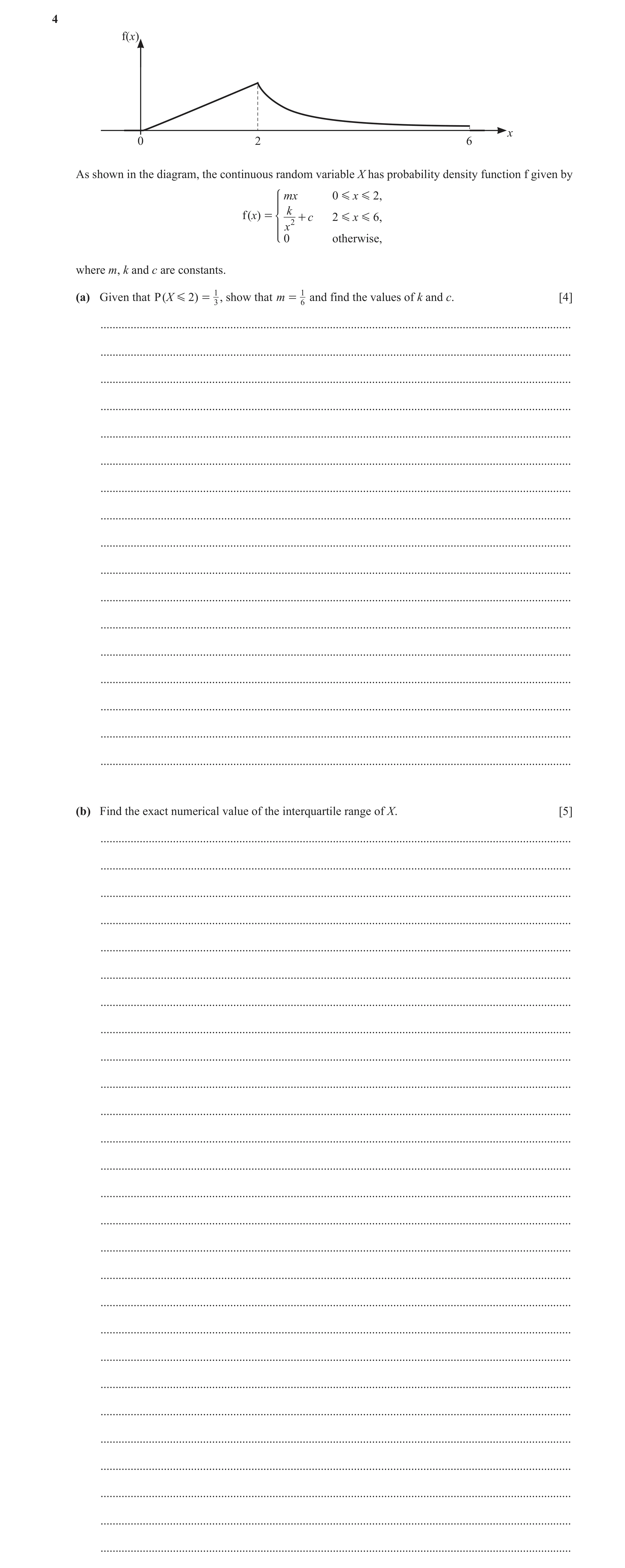
4 f(x) x 0 2 6 As shown in the diagram, the continuous random variable X has probability density function f given by mx 0 G x G 2 , k f ( x) = + c 2 G x G 6, 2 x * 0 otherwise, where m, k and c are constants. = (a) Given that P ( X G 2 ) = 13 , show that m 1 6 and find the values of k and c. [4] … … … … … … … … … … … … … … … … … (b) Find the exact numerical value of the interquartile range of X. [5] … … … … … … … … … … … … … … … … … … … … … … … … … … …
9 marks
Mark scheme: 4(a) 2 2 B1 AG 1 P(X ⩽ 2) = , so mx = 1 Reasoning required. 3 2 0 3 4 1 1 m = , m = 2 3 6 6 6 M1 Attempt to integrate and correct use of correct limits to k 2 k 1 2 + c so − + cx = 4c + k = or k + 12c = 2 form linear equation in k and c. dx = 3 x 3 3 x 2 2 2 k 1 k M1 Matching at x = 2 . Also, 2 m = + c or = + c or 3k + 12c = 4 4 3 4 1 A1 Solve, k = 1, c = 12 4 4(b) L B1 1 1 LQ: xdx = , L = 3 6 4 0 U M1 Or find and use CDF. May be in terms of m. 1 k 3 UQ: dx = + c + 3 4 x 2 2 k k 5 M1 Attempt at integral and correct use of correct limits. − + Uc + − 2c = Simplify to quadratic equation, may be in terms of k and U 2 12 2 c. U − U − 12 = 0 U = 4 A1 IQR = 4 − 3 A1 FT FT their UQ – their LQ, exact values only. 5
This question in 9231/41 Oct/Nov 2023
Q27 · F(x) x 0 4 6 The diagram shows the continuous random variable X with probability density… 9231/42 Oct/Nov 2023
4 f(x) x 0 4 6 The diagram shows the continuous random variable X with probability density function f given by Z ] 1 3 128 ( 4 ax - bx ) 0 G x G 4, ]] f ( x) = [ c 4 G x G 6 , ] ] 0 otherwise, \ where a, b and c are constants. The upper quartile of X is equal to 4. (a) Show that c = 18 and find the values of a and b. [4] … … … … … … … … … … … … … … … … (b) Find the exact value of the median of X. [3] … … … … … … … … … … … … … … (c) Find E ( X ), giving your answer correct to 2 decimal places. [3] … … … … … … … … … … … …
10 marks
Mark scheme: 4(a) 6 B1 AG. 1 1 1 UQ = 4 so , c = : c 6 − 4 = Some indication of reasoning required. cdx = 4 4 8 4 4 M1 Integrate and use correct limits to form equation 1 3 3 1 2 b 4 3 4 ax − bx dx = , 2 ax − x = , 32a − 64b = 96 in a and b. ( ) 128 4 128 4 4 0 Equate at x = 4: a − 4b = 1 M1 Solve: a = 5, b = 1 A1 4 4(b) m M1* Attempt at integral and use of correct limits. 1 3 1 20 x − x dx = Could be in terms of a , b, c ( ) 128 2 0 Or attempt at relevant part of CDF and set OR 1 F ( m ) = . 1 2 b 4 5 2 1 4 2 ax − x = x − x 2 F ( x ) = 128 4 64 512 Could be in terms of a , b, c . m 4 − 40m 2 + 256 = 0 M1 Simplify to quartic. Could be in terms of a , b, c . m = 2 2 A1 Positive answer only. 3 4(c) Their PDF multiplied by x with correct limits. 1 4 32 72 6 1 12 M1 X = 20 x − x dx + x dx E( ) 128 8 Could be in terms of a , b, c . 0 4 4 6 5 9 3 M1 Correct use of correct limits in their integral. 1 2 2 2 1 2 8 x − x + x Could be in terms of a, b, c. 128 9 0 12 4 May be implied by correct final answer. 1 8 1 10 1 4 1 A1 CAO 2 − 2 + 6 6 − 8 = + 6 = 1.67 ( ) 1.67 following (first) M0 SC B2 128 9 12 9 2 3
This question in 9231/42 Oct/Nov 2023
Q28 · F(x) x 0 2 6 As shown in the diagram, the continuous random variable X has probability… 9231/43 Oct/Nov 2023
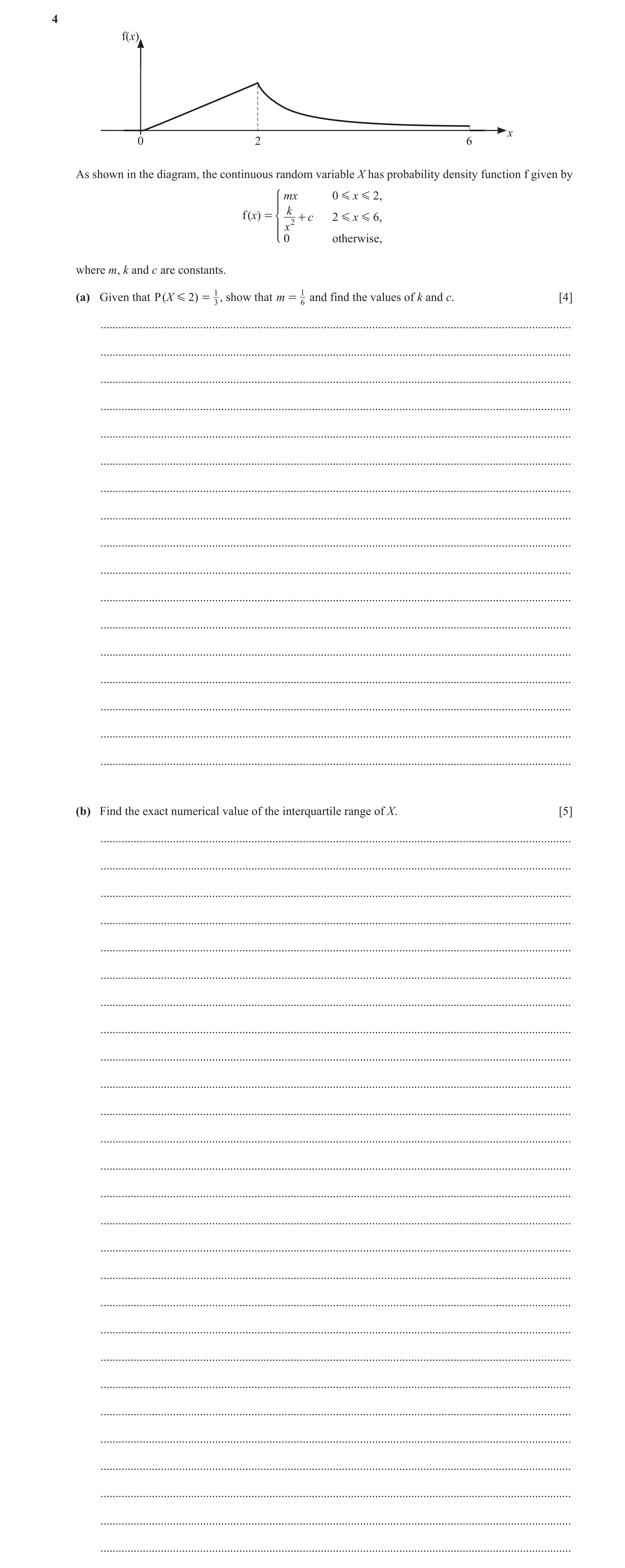
4 f(x) x 0 2 6 As shown in the diagram, the continuous random variable X has probability density function f given by mx 0 G x G 2 , k f ( x) = + c 2 G x G 6, 2 x * 0 otherwise, where m, k and c are constants. = (a) Given that P ( X G 2 ) = 13 , show that m 1 6 and find the values of k and c. [4] … … … … … … … … … … … … … … … … … (b) Find the exact numerical value of the interquartile range of X. [5] … … … … … … … … … … … … … … … … … … … … … … … … … … …
9 marks
Mark scheme: 4(a) 2 2 B1 AG 1 P(X ⩽ 2) = , so mx = 1 Reasoning required. 3 2 0 3 4 1 1 m = , m = 2 3 6 6 6 M1 Attempt to integrate and correct use of correct limits to k 2 k 1 2 + c so − + cx = 4c + k = or k + 12c = 2 form linear equation in k and c. dx = 3 x 3 3 x 2 2 2 k 1 k M1 Matching at x = 2 . Also, 2 m = + c or = + c or 3k + 12c = 4 4 3 4 1 A1 Solve, k = 1, c = 12 4 4(b) L B1 1 1 LQ: xdx = , L = 3 6 4 0 U M1 Or find and use CDF. May be in terms of m. 1 k 3 UQ: dx = + c + 3 4 x 2 2 k k 5 M1 Attempt at integral and correct use of correct limits. − + Uc + − 2c = Simplify to quadratic equation, may be in terms of k and U 2 12 2 c. U − U − 12 = 0 U = 4 A1 IQR = 4 − 3 A1 FT FT their UQ – their LQ, exact values only. 5
This question in 9231/43 Oct/Nov 2023
Q29 · The continuous random variable X has probability density function f given by x 2 ( 4 - x… 9231/41 May/June 2024
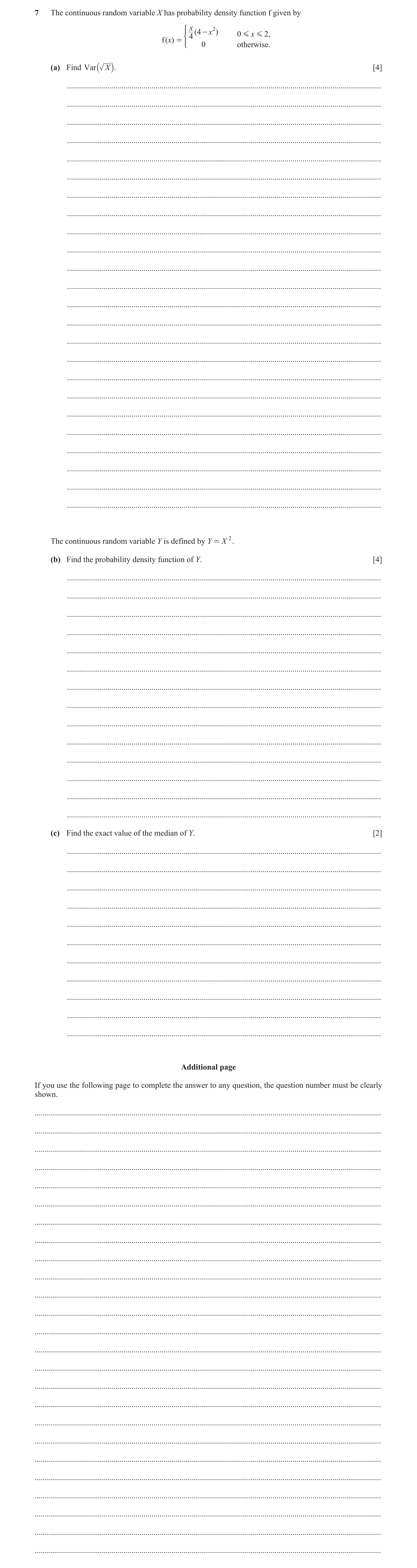
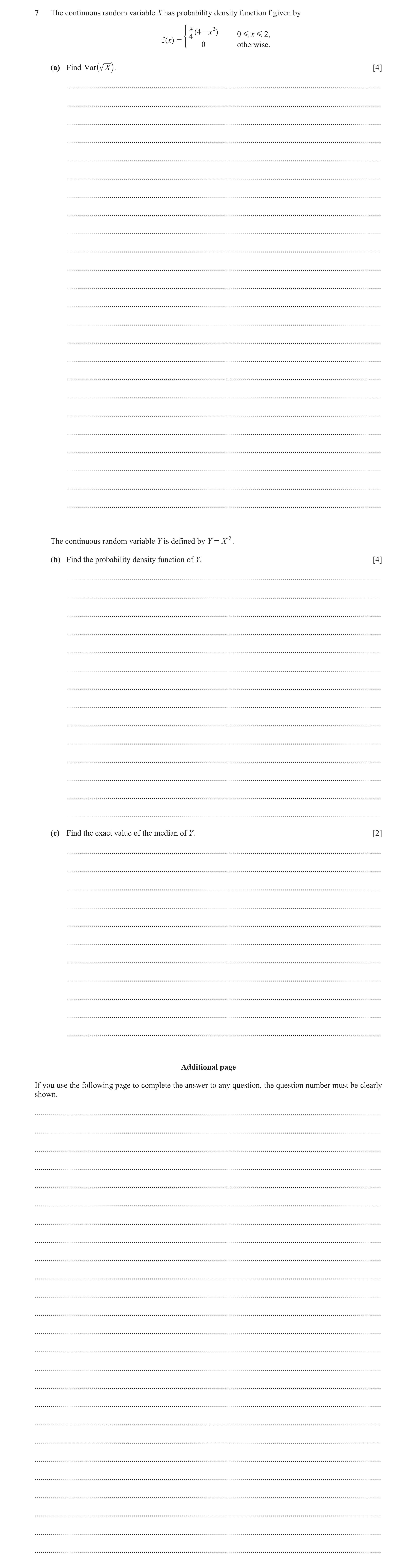
7 The continuous random variable X has probability density function f given by x 2 ( 4 - x ) 0 G x G 2 , 4 f ( x) = * 0 otherwise. (a) Find Var X [4] ` j. … … … … … … … … … … … … … … … … … … … … … … … … The continuous random variable Y is defined by Y = X 2 . (b) Find the probability density function of Y. [4] … … … … … … … … … … … … … … (c) Find the exact value of the median of Y. [2] … … … … … … … … … … … Additional page If you use the following page to complete the answer to any question, the question number must be clearly shown. … … … … … … … … … … … … … … … … … … … … … … … … …
10 marks
Mark scheme: 7(a) 2 4 0 2, f 4 0 otherwise. x x x x (E(X) =) 2 1 1 4 1 16 2 4 3 5 4 4 3 5 15 0 4 d x x x x x ( = 1.067) (E( 2 2 1 1 8 2 32 1.5 7.2 2.5 4.5 4 4 5 9 45 0 0 ) ) 4 d 2 1.005 7 X x x x x x M1 Integration, correct powers required, ignore limits. Var( 2 ) E X E X X used M1 Correct formula used following attempt at integration of both terms. 2 16 32 15 45 2 0.0553 A1 112 2025 4 Question Answer Marks Guidance 7(b) F(x) = 2 4 1 8 16 x x 0 2 x B1 G(y) = 2 1 8 16 y y [ 0 4] y M1 Change variable in their F(x). 1 8 2 0 4 16 g y y y M1 Differentiate their G(y) . 1 8 2 0 4, 16 0 otherwise. y y g y A1 Complete and correct. 4 7(c) 2 1 1 8 16 2 m m M1 Equate their G(y) to 1 2 . 2 [ 8 8 0,] 4 2 2 m m m A1 Single answer in an exact form. 2
This question in 9231/41 May/June 2024
Q30 · The continuous random variable X has probability density function f given by x 2 ( 4 - x… 9231/42 May/June 2024
7 The continuous random variable X has probability density function f given by x 2 ( 4 - x ) 0 G x G 2 , 4 f ( x) = * 0 otherwise. (a) Find Var X [4] ` j. … … … … … … … … … … … … … … … … … … … … … … … … The continuous random variable Y is defined by Y = X 2 . (b) Find the probability density function of Y. [4] … … … … … … … … … … … … … … (c) Find the exact value of the median of Y. [2] … … … … … … … … … … … Additional page If you use the following page to complete the answer to any question, the question number must be clearly shown. … … … … … … … … … … … … … … … … … … … … … … … … …
10 marks
Mark scheme: 7(a) 2 4 0 2, f 4 0 otherwise. x x x x (E(X) =) 2 1 1 4 1 16 2 4 3 5 4 4 3 5 15 0 4 d x x x x x ( = 1.067) (E( 2 2 1 1 8 2 32 1.5 7.2 2.5 4.5 4 4 5 9 45 0 0 ) ) 4 d 2 1.005 7 X x x x x x M1 Integration, correct powers required, ignore limits. Var( 2 ) E X E X X used M1 Correct formula used following attempt at integration of both terms. 2 16 32 15 45 2 0.0553 A1 112 2025 4 Question Answer Marks Guidance 7(b) F(x) = 2 4 1 8 16 x x 0 2 x B1 G(y) = 2 1 8 16 y y [ 0 4] y M1 Change variable in their F(x). 1 8 2 0 4 16 g y y y M1 Differentiate their G(y) . 1 8 2 0 4, 16 0 otherwise. y y g y A1 Complete and correct. 4 7(c) 2 1 1 8 16 2 m m M1 Equate their G(y) to 1 2 . 2 [ 8 8 0,] 4 2 2 m m m A1 Single answer in an exact form. 2
This question in 9231/42 May/June 2024
Q31 · The continuous random variable X has probability density function f given by kx 3 0 G x 1… 9231/41 Oct/Nov 2024
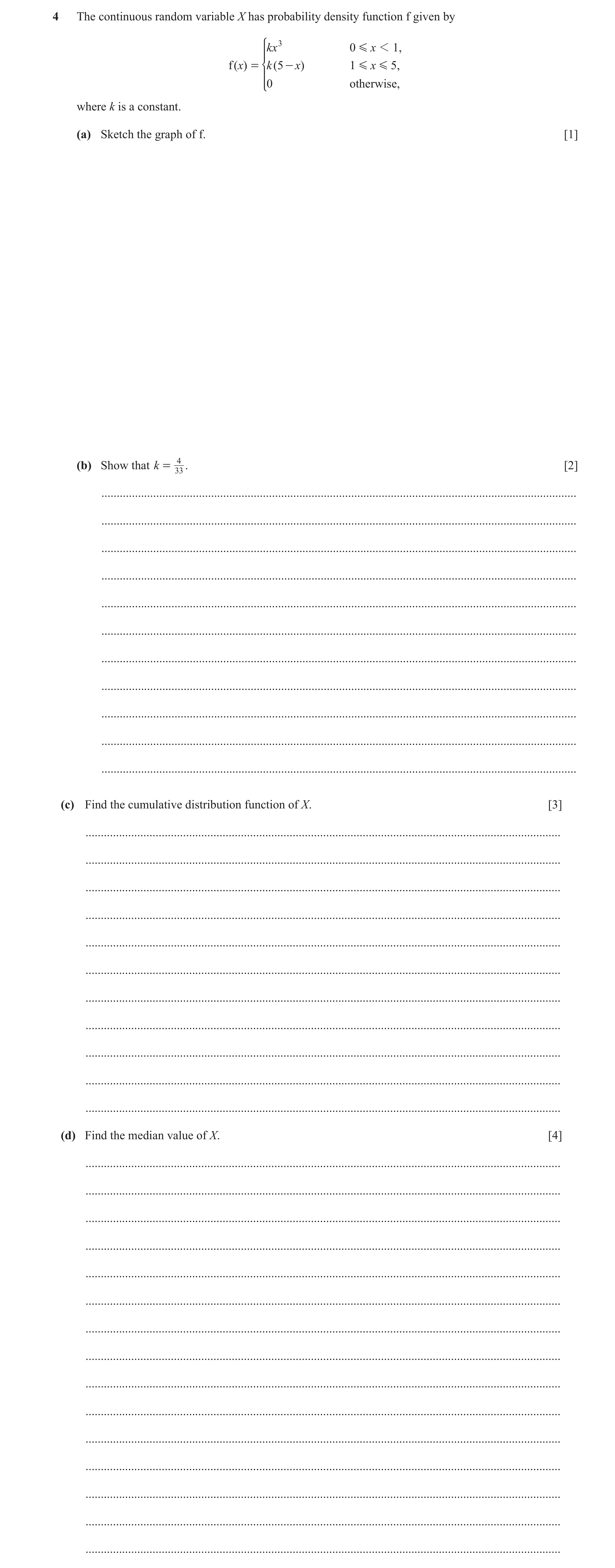
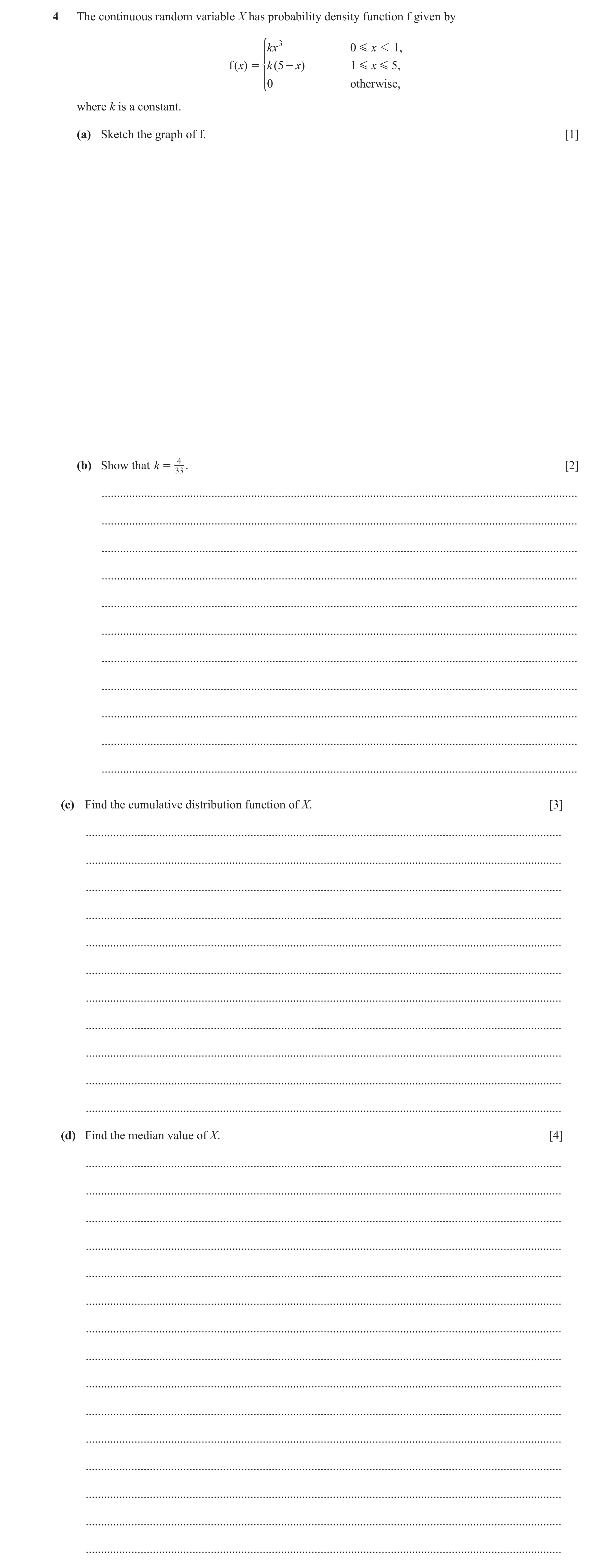
4 The continuous random variable X has probability density function f given by kx 3 0 G x 1 1 , f ( x) = *k ( 5 - x) 1 G x G 5 , 0 otherwise, where k is a constant. (a) Sketch the graph of f. [1] (b) Show that k = 4 . [2] 33 … … … … … … … … … … … (c) Find the cumulative distribution function of X. [3] … … … … … … … … … … … (d) Find the median value of X. [4] … … … … … … … … … … … … … … …
10 marks
Mark scheme: 4(a) Correct sketch. B1 Label 1 and 5 on x-axis, ignore labels, if any, on y-axis. 1 4(b) kx 4 k B1 For either part correct. with limits 0 and 1 gives 4 4 x 2 k 5 x − with limits 1 and 5 gives 8k 2 k 4 B1 AG + 8k = 1, k = 4 33 2 4(c) M1 Integrate both parts. 0 x 0 A1 Middle two parts correct AEF. 1 4 x 0 ≤ x 1 A1 0 and 1 correct. 33 F( x ) = 4 1 2 17 5 x − x − 1 ≤≤x 5 33 2 4 1 x 5. 3 4(d) 1 3 m 1 M1* Or integrate m to 5. Or use F(x) = 0.5. 0kx dx + 1 k ( 5 − x ) dx = 2 4 1 1 2 1 1 4 25 1 2 1 M1 Must be a quadratic in m. + 5m − m − 5 + = or − 5m + m = 33 4 2 2 2 33 2 2 2 4 1 2 17 1 or 5 m − m − = 33 2 4 2 4 m 2 − 40 m + 67 = 0 *DM1 1 A1 m = 10 − 33 = 2.13 ( ) 2 4
This question in 9231/41 Oct/Nov 2024
Q32 · The continuous random variable X has probability density function f given by kx 3 0 G x 1… 9231/43 Oct/Nov 2024
4 The continuous random variable X has probability density function f given by kx 3 0 G x 1 1 , f ( x) = *k ( 5 - x) 1 G x G 5 , 0 otherwise, where k is a constant. (a) Sketch the graph of f. [1] (b) Show that k = 4 . [2] 33 … … … … … … … … … … … (c) Find the cumulative distribution function of X. [3] … … … … … … … … … … … (d) Find the median value of X. [4] … … … … … … … … … … … … … … …
10 marks
Mark scheme: 4(a) Correct sketch. B1 Label 1 and 5 on x-axis, ignore labels, if any, on y-axis. 1 4(b) kx 4 k B1 For either part correct. with limits 0 and 1 gives 4 4 x 2 k 5 x − with limits 1 and 5 gives 8k 2 k 4 B1 AG + 8k = 1, k = 4 33 2 4(c) M1 Integrate both parts. 0 x 0 A1 Middle two parts correct AEF. 1 4 x 0 ≤ x 1 A1 0 and 1 correct. 33 F( x ) = 4 1 2 17 5 x − x − 1 ≤≤x 5 33 2 4 1 x 5. 3 4(d) 1 3 m 1 M1* Or integrate m to 5. Or use F(x) = 0.5. 0kx dx + 1 k ( 5 − x ) dx = 2 4 1 1 2 1 1 4 25 1 2 1 M1 Must be a quadratic in m. + 5m − m − 5 + = or − 5m + m = 33 4 2 2 2 33 2 2 2 4 1 2 17 1 or 5 m − m − = 33 2 4 2 4 m 2 − 40 m + 67 = 0 *DM1 1 A1 m = 10 − 33 = 2.13 ( ) 2 4
This question in 9231/43 Oct/Nov 2024
Q33 · The continuous random variable X has probability density function f given by kx 0 G x 1… 9231/44 May/June 2025
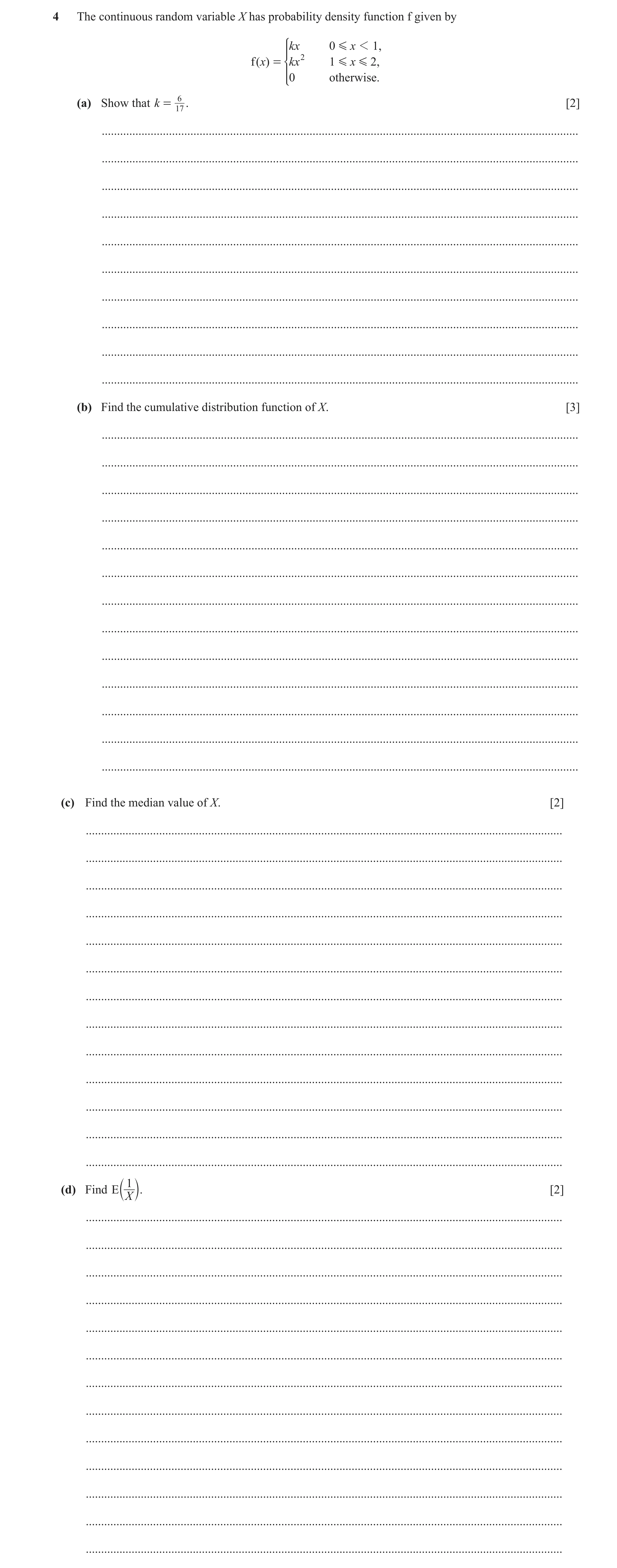
4 The continuous random variable X has probability density function f given by kx 0 G x 1 1, f ( x) = *kx 2 1 G x G 2 , 0 otherwise. (a) Show that k = 6 . [2] 17 … … … … … … … … … … (b) Find the cumulative distribution function of X. [3] … … … … … … … … … … … … … (c) Find the median value of X. [2] … … … … … … … … … … … … … 1 (d) Find Eb l. [2] X … … … … … … … … … … … … …
9 marks
Mark scheme: kx dx = 1 kx + kx = 1 2 3 0 14(a) 10 2 2 1 2 1 1 3 2 M1 Linear equation in terms of k formed following attempt to kx d x + 1 integrate (all powers correct) and use of correct limits. 1 1 for first region. 2 1 k ) 2 k + 13 k ( 8 − 1) = 1 May consider area of triangle ( 17 6 k = 1, k = 176 A1 AG, shown convincingly. No errors seen. 2 4(b) 0 x 0 M1 Attempt to integrate both parts, all powers correct, condone 3 2 missing c . x 0 ≤ x 1 Sight of expressions for 0 ≤ x 1 and 1 ≤ x ≤ 2 sufficient. F ( x ) = 17 2 3 1 ≤ x ≤ 2 17 x + 17 1 1 x 2 A1 Both parts correct with c = 171 . Sight of expressions for 0 ≤ x 1 and 1 ≤ x ≤ 2 sufficient. A1 All correct, fully defined including domain. Domain must cover all reals, may overlap at boundaries. 3 1 ≤ m ≤ 2 and their F ( x ) (or areas) to form equation with 0.5.4(c) F ( m ) = 2 so 172 m 3 + 171 = 12 M1 Use 1 3 15 3 15 A1 FT FT their non-zero c , to obtain m with 1 ≤ m ≤ 2 . m = 4 , m = 4 = 1.55 2 2 M1 Correct method and attempt to integrate both parts. All powers4(d) 1 1 6 1 2 6 2 1 6 1 6 1 2 x correct, limits not required. E = 17 x dx + 17 x dx = 17 0 + 17 2 x 1 X 0 x 1 x 6 15 1 = 0.882 A1 CWO, AWRT 0.882. (1 + 2 − 17 2 ) = 17 2
This question in 9231/44 May/June 2025
Q34 · A continuous random variable X has probability density function f given by Z ] 1 x 0 G x… 9231/41 Oct/Nov 2025
5 A continuous random variable X has probability density function f given by Z ] 1 x 0 G x 1 4 , ]] 16 f ( x) = [ 1 4 G x G ,9 ] k x ] 0 otherwise, \ where k is a constant. (a) Show that k = 3 . [2] … … … … … … … … (b) Find the median value of X. [3] … … … … … … … … … … … The random variable Y is defined by Y = X . (c) Find the probability density function of Y. [5] … … … … … … … … … … … … … … … … … … … … … … … … … …
10 marks
Mark scheme: 45(a) M1 Equation in terms of k formed following attempt to integrate with 9 2 1 1 2 x 3 + 2 x = 1 correct limits. 4 16 3 k 0 1 2 ( 8 − 0 ) + ( 3 − 2 ) = 1 24 k OR 1 2 + = 1 3 k 2 A1 AG, no errors seen. = 2, k = 3 k 3 2 15(b) 1 4 1 m − 2 1 *M1 Use of 4 m 9 to form equation equal to 0.5, OE. 16 0 x d x + 3 4 x dx = 2 Equation may be in terms of k. OR 1 9 − 12 3 m x d x = 0.5 1 m − 2 = 12 DM1 Integrate and form an equation in m . 3 + 32 ( ) OR 2 3 − m = 12 3 ( ) m = 1681 [ = 5.0625] A1 Accept AWRT 5.06. 3 M1 Attempt to integrate both parts, limits not required.5(c) 2 0 ≤ x 4 241 x 3 F ( x ) = 1 May be seen in part 5(a). ≤ x ≤ 9 23 x 2 − 1 4 B1 For constant –1 obtained in expression for 4 ≤ x ≤ 9 . May be seen in part 5(a). ≤ y 2 M1 For changing to y . 241 y 3 0 G ( y ) = Limits not required. ≤ y ≤ 3 23 y − 1 2 1 ≤ y 2 M1 For differentiation, limits not required. 8 y 2 0 2 ≤ y ≤ 3 g ( y ) = 3 2 A1 Fully correct with correct domain covering all reals. 0 otherwise Alternative method for question 5(c) Using chain rule (or inverse function): M1 M1 for changing to y . 2 d 2 2 y . y = 2 yf y G ( y ) = F ( ) so g ( y ) = F ( ) ( ) dy A1 M2 y 2 twice, limits not required. 2 y 1 y 2 0 ≤ y 2 Use of g ( y ) = 2 yf ( ) ) ( 16 M1 for one expression. g ( y ) = 1 2 y 2 ≤ y ≤ 3 2 3 y 1 ≤ y 2 A1 Fully correct with correct domain covering all reals. 8 y 2 0 2 ≤ y ≤ 3 g ( y ) = 3 2 0 otherwise 5
This question in 9231/41 Oct/Nov 2025
Q35 · A continuous random variable X has cumulative distribution function F given by Z ]0 x 1 1… 9231/42 Oct/Nov 2025
4 A continuous random variable X has cumulative distribution function F given by Z ]0 x 1 1 , ] 1 x + a 1 G x 1 4, F ( x) = [ 51 2 x + b 4 G x G 6, 50 ]] 1 x 2 6, \ where a and b are constants. (a) Find the value of a and the value of b. [2] … … … … … … … … (b) Find the probability density function of X. [2] … … … … … … … … … … … … … (c) Given that E ( X ) = 529 , find Var (X ). [3] 150 … … … … … … … … … … … (d) Find the 10th and 90th percentiles of X. [3] … … … … … … … … … … … … … … …
10 marks
Mark scheme: 4(a) a = − 15 B1 b = 257 B1 2 ≤ x 4, M1 Attempt at differentiating both parts.4(b) 15 1 1 ≤ x ≤ 6, f ( x ) = 25 x 4 A1 All correct, fully defined including domain. 0 otherwise. Domain must cover all reals, must not overlap at boundaries. 2 4 64(c) M1 Attempt to integrate x 2f ( x ) with correct limits. E X 2 x 3 dx = 1 x 3 + 1 x 4 ( ) 15 100 1 4 = 15 14 x 2 dx + 251 46 Can be implied by answer of 735 or 14.6. 73 529 2 M1 2 . Variance formula used with their E X ( ) Var ( X ) = 5 − ( 150 ) 2.16 A1 3 4(d) 10th percentile: 15 x − 15 = 101 M1 Award M1 for a correct method to find at least one of the 10th or 90th percentile. 1 2 7 9 90th percentile: 50 x + 25 = 10 FT their a and b. 10th percentile = 1.5 A1 90th percentile = 31 A1 AWRT 5.57. 3
This question in 9231/42 Oct/Nov 2025
Q36 · A continuous random variable X has probability density function f given by Z ] 1 x 0 G x… 9231/43 Oct/Nov 2025
5 A continuous random variable X has probability density function f given by Z ] 1 x 0 G x 1 4 , ]] 16 f ( x) = [ 1 4 G x G ,9 ] k x ] 0 otherwise, \ where k is a constant. (a) Show that k = 3 . [2] … … … … … … … … (b) Find the median value of X. [3] … … … … … … … … … … … The random variable Y is defined by Y = X . (c) Find the probability density function of Y. [5] … … … … … … … … … … … … … … … … … … … … … … … … … …
10 marks
Mark scheme: 45(a) M1 Equation in terms of k formed following attempt to integrate with 9 2 1 1 2 x 3 + 2 x = 1 correct limits. 4 16 3 k 0 1 2 ( 8 − 0 ) + ( 3 − 2 ) = 1 24 k OR 1 2 + = 1 3 k 2 A1 AG, no errors seen. = 2, k = 3 k 3 2 15(b) 1 4 1 m − 2 1 *M1 Use of 4 m 9 to form equation equal to 0.5, OE. 16 0 x d x + 3 4 x dx = 2 Equation may be in terms of k. OR 1 9 − 12 3 m x d x = 0.5 1 m − 2 = 12 DM1 Integrate and form an equation in m . 3 + 32 ( ) OR 2 3 − m = 12 3 ( ) m = 1681 [ = 5.0625] A1 Accept AWRT 5.06. 3 M1 Attempt to integrate both parts, limits not required.5(c) 2 0 ≤ x 4 241 x 3 F ( x ) = 1 May be seen in part 5(a). ≤ x ≤ 9 23 x 2 − 1 4 B1 For constant –1 obtained in expression for 4 ≤ x ≤ 9 . May be seen in part 5(a). ≤ y 2 M1 For changing to y . 241 y 3 0 G ( y ) = Limits not required. ≤ y ≤ 3 23 y − 1 2 1 ≤ y 2 M1 For differentiation, limits not required. 8 y 2 0 2 ≤ y ≤ 3 g ( y ) = 3 2 A1 Fully correct with correct domain covering all reals. 0 otherwise Alternative method for question 5(c) Using chain rule (or inverse function): M1 M1 for changing to y . 2 d 2 2 y . y = 2 yf y G ( y ) = F ( ) so g ( y ) = F ( ) ( ) dy A1 M2 y 2 twice, limits not required. 2 y 1 y 2 0 ≤ y 2 Use of g ( y ) = 2 yf ( ) ) ( 16 M1 for one expression. g ( y ) = 1 2 y 2 ≤ y ≤ 3 2 3 y 1 ≤ y 2 A1 Fully correct with correct domain covering all reals. 8 y 2 0 2 ≤ y ≤ 3 g ( y ) = 3 2 0 otherwise 5
This question in 9231/43 Oct/Nov 2025
![Question 1: The continuous random variable X has probability density function f given by Z 3 ] 16 2 - x 0 G x 1 1, ` j ] 3 f ( x) = [ 1 G x G 9, 16 x ]…](https://img.pastlit.com/crops/82035ff5-095f-45e2-af6d-b9981dae6f48/q3.webp)
![Question 2: The continuous random variable X has probability density function f given by Z 3 ] 16 2 - x 0 G x 1 1, ` j ] 3 f ( x) = [ 1 G x G 9, 16 x ]…](https://img.pastlit.com/crops/5b3aca79-bcc1-4fc7-84be-f15af87ab175/q3.webp)
![Question 10: The continuous random variable X has cumulative distribution function F given by Z ] 0 x 1 - 1, ]] 1 2 2 ( 1 + x) - 1 G x G 0 , F ( x) = [ …](https://img.pastlit.com/crops/ade3312d-ba29-47f9-9730-056c796d06e3/q2.webp)
![Question 12: The continuous random variable X has cumulative distribution function F given by Z ] 0 x 1 - 1, ]] 1 2 2 ( 1 + x) - 1 G x G 0 , F ( x) = [ …](https://img.pastlit.com/crops/02f7968f-da10-4912-aa68-d6ea98ac9a56/q2.webp)
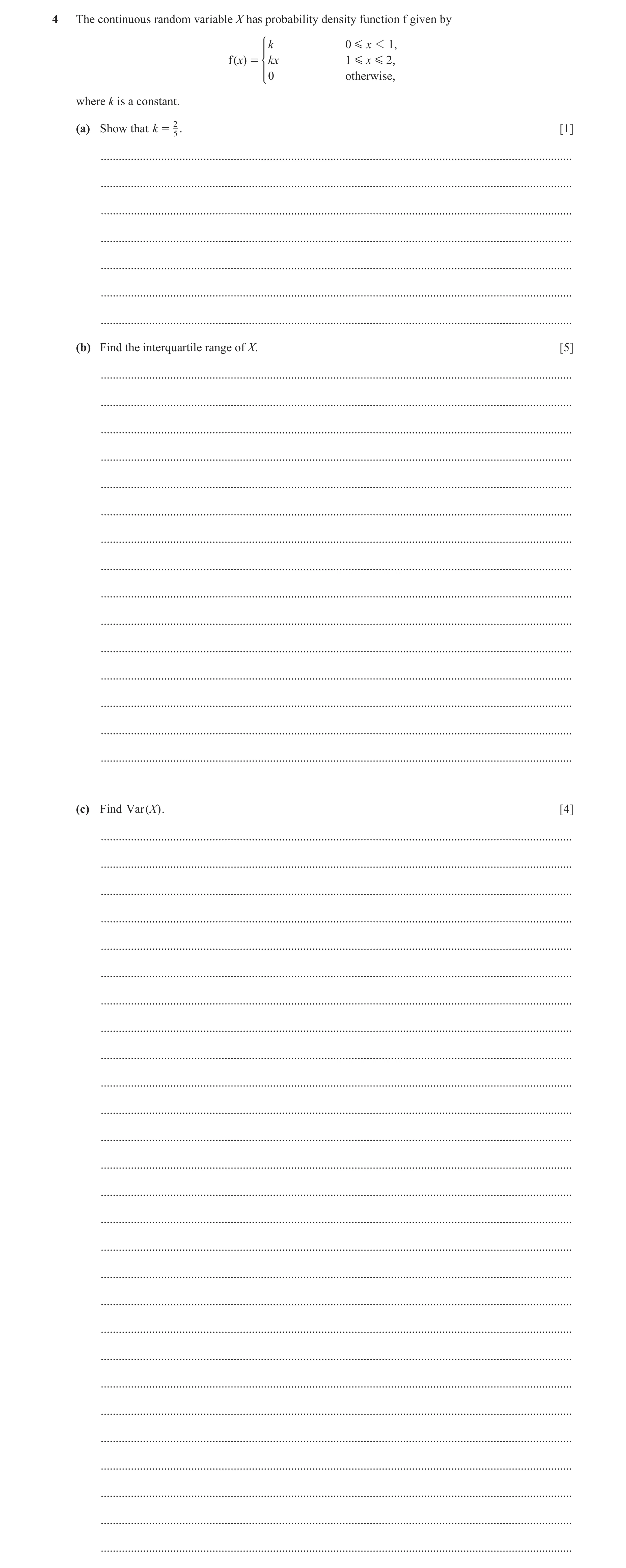
![Question 27: f(x) x 0 4 6 The diagram shows the continuous random variable X with probability density function f given by Z ] 1 3 128 ( 4 ax - bx ) 0 G …](https://img.pastlit.com/crops/8670bbfd-00a6-44d3-8745-17a888e398c5/q4.webp)
![Question 34: A continuous random variable X has probability density function f given by Z ] 1 x 0 G x 1 4 , ]] 16 f ( x) = [ 1 4 G x G ,9 ] k x ] 0 othe…](https://img.pastlit.com/crops/e2e7f183-7c8d-4a56-9b62-afffb6bed5f8/q5.webp)
![Question 35: A continuous random variable X has cumulative distribution function F given by Z ]0 x 1 1 , ] 1 x + a 1 G x 1 4, F ( x) = [ 51 2 x + b 4 G …](https://img.pastlit.com/crops/b3227f57-6bfe-4faa-bf07-19a71657b8f8/q4.webp)
![Question 36: A continuous random variable X has probability density function f given by Z ] 1 x 0 G x 1 4 , ]] 16 f ( x) = [ 1 4 G x G ,9 ] k x ] 0 othe…](https://img.pastlit.com/crops/e596c1d7-252f-47af-927c-82bd422aaecb/q5.webp)
 8
8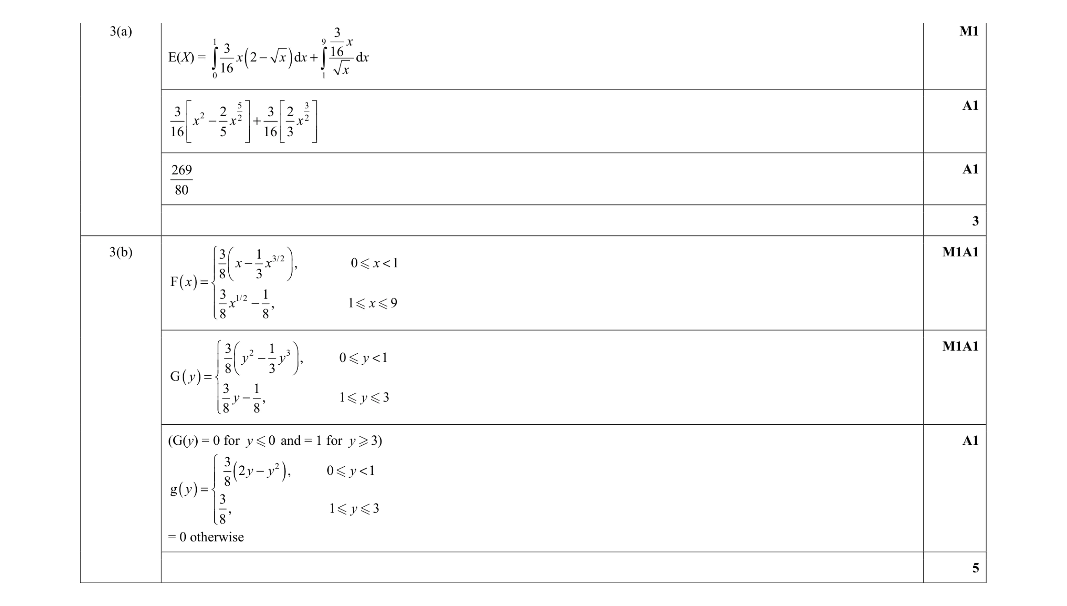 8
8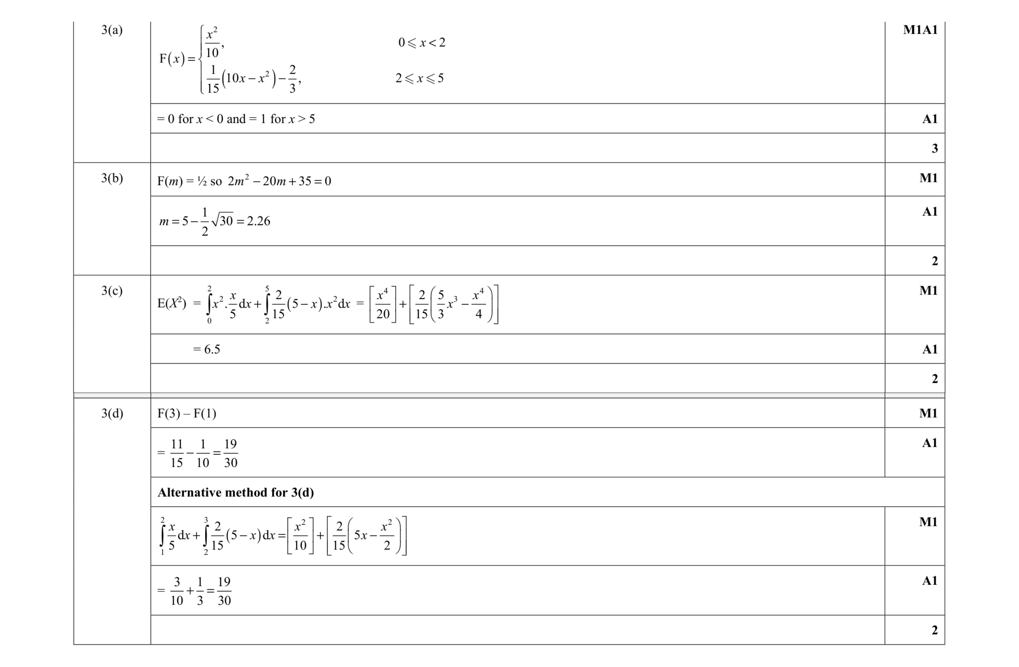 9
9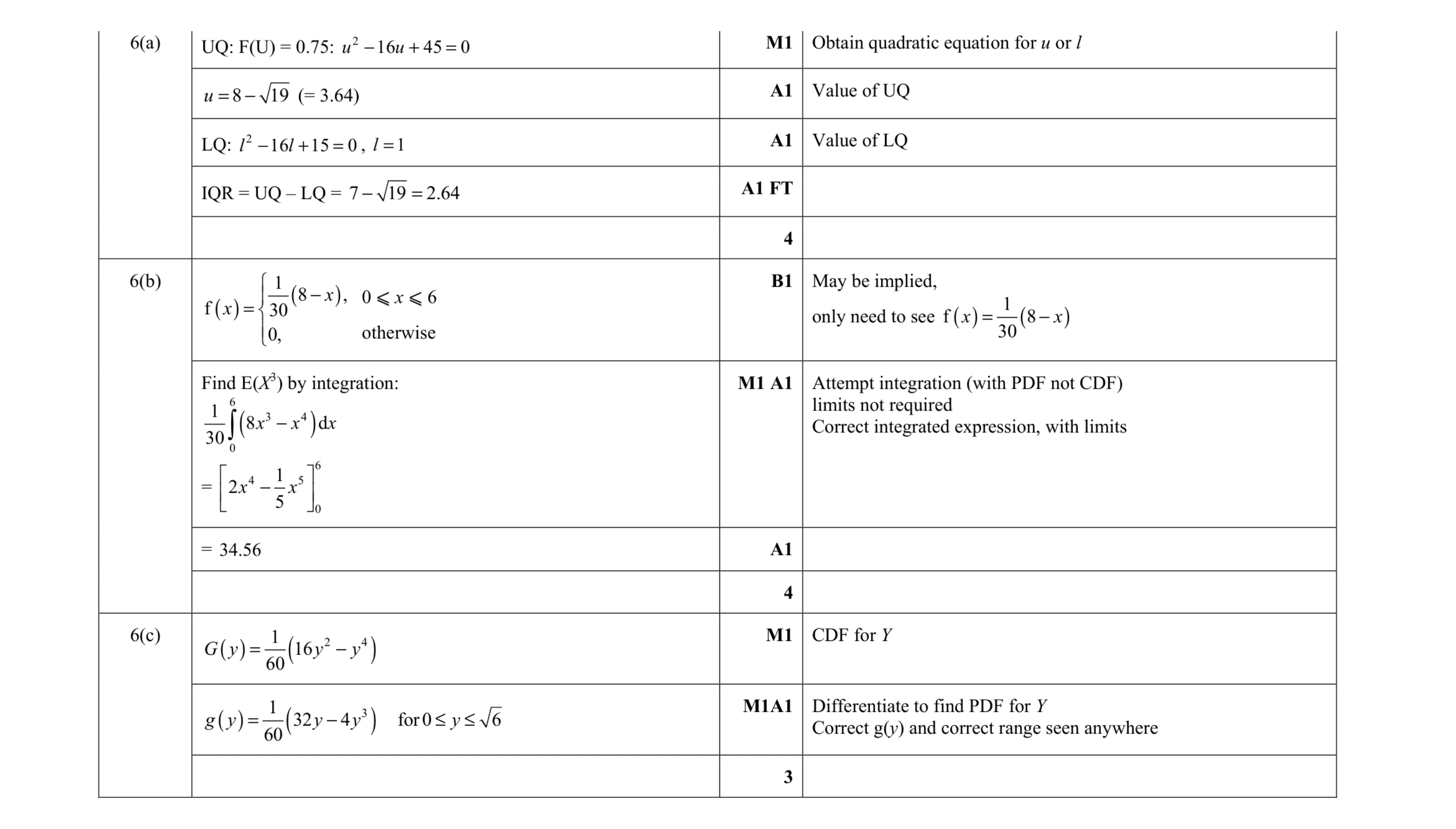 11
11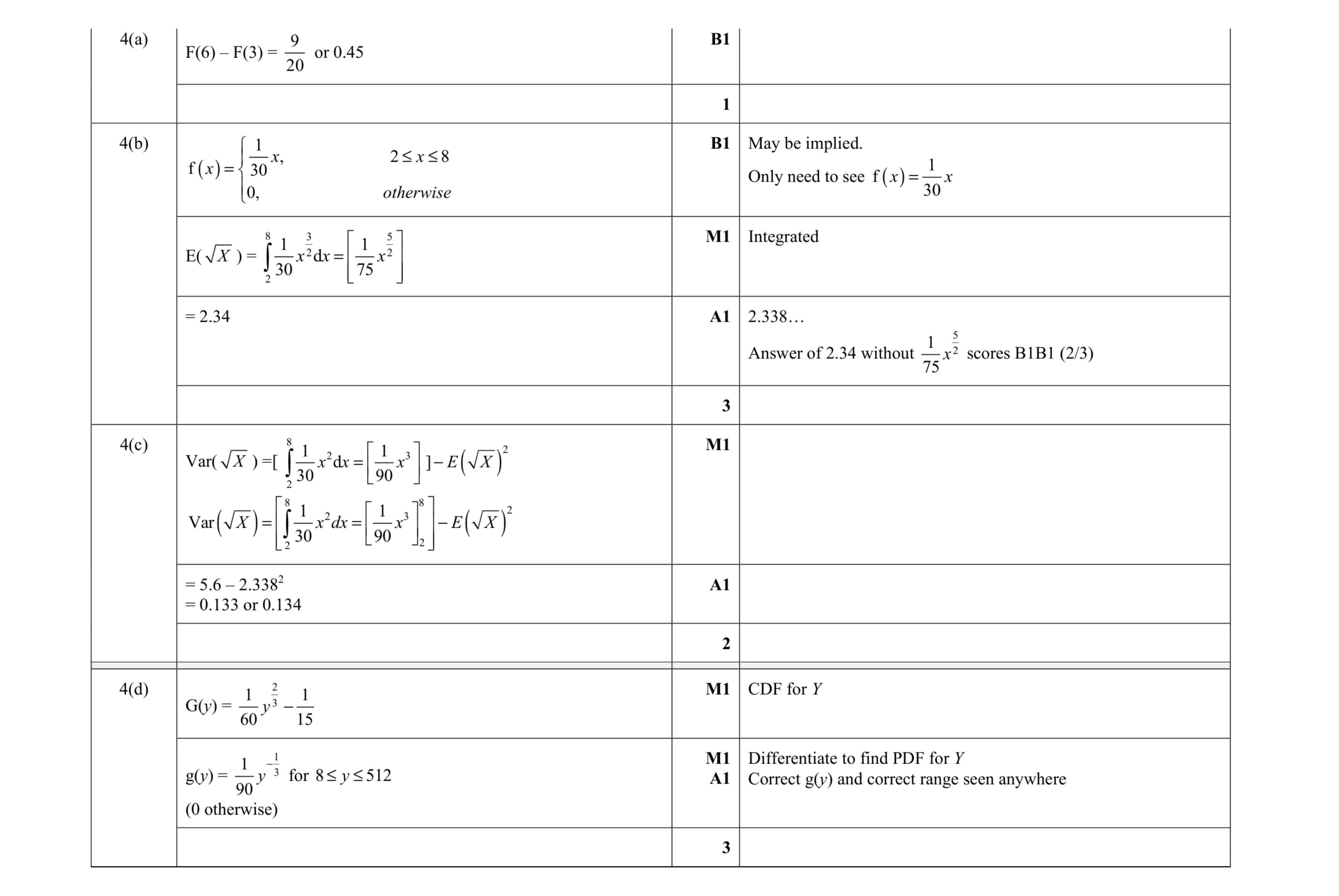 9
9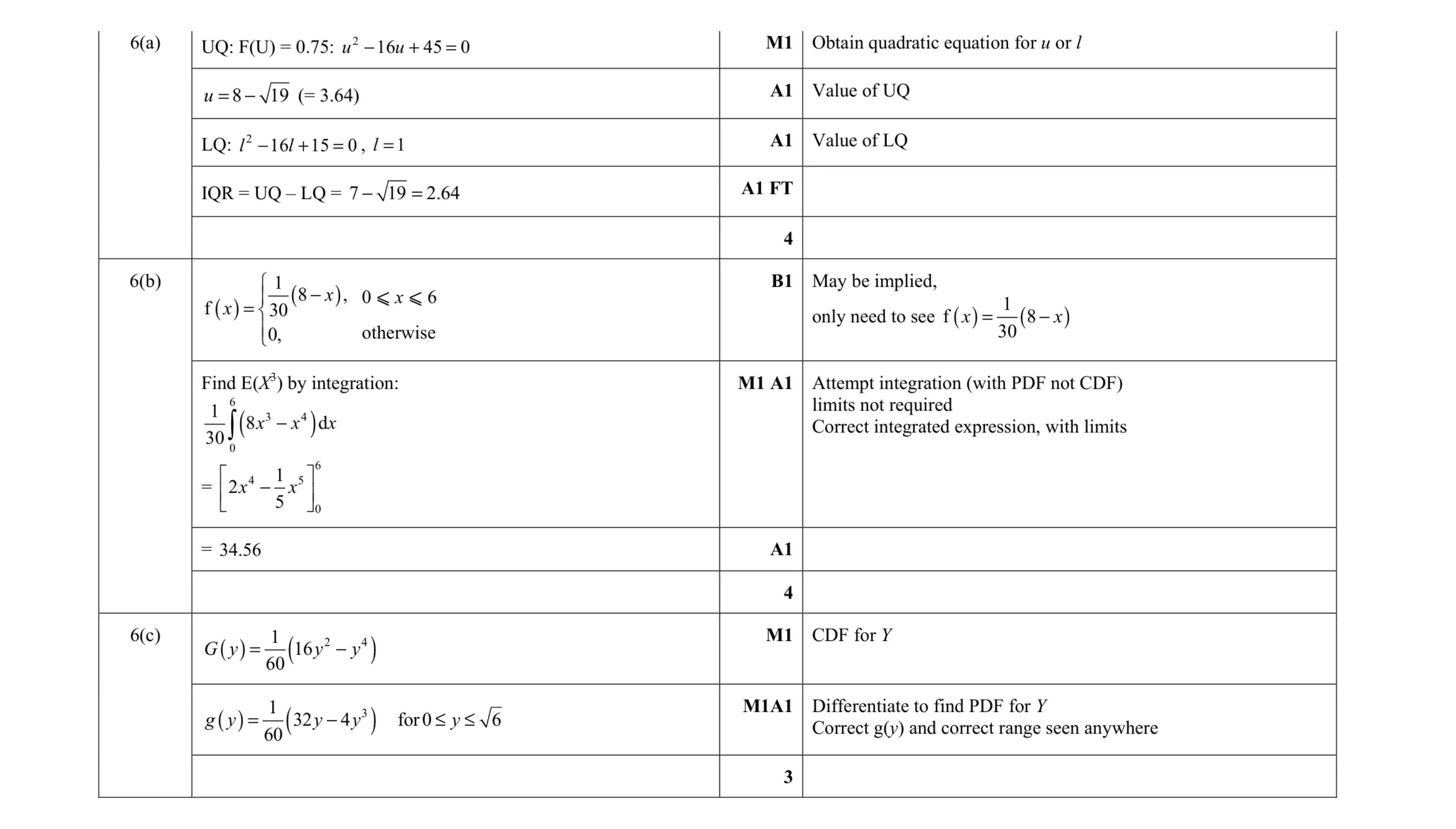 11
11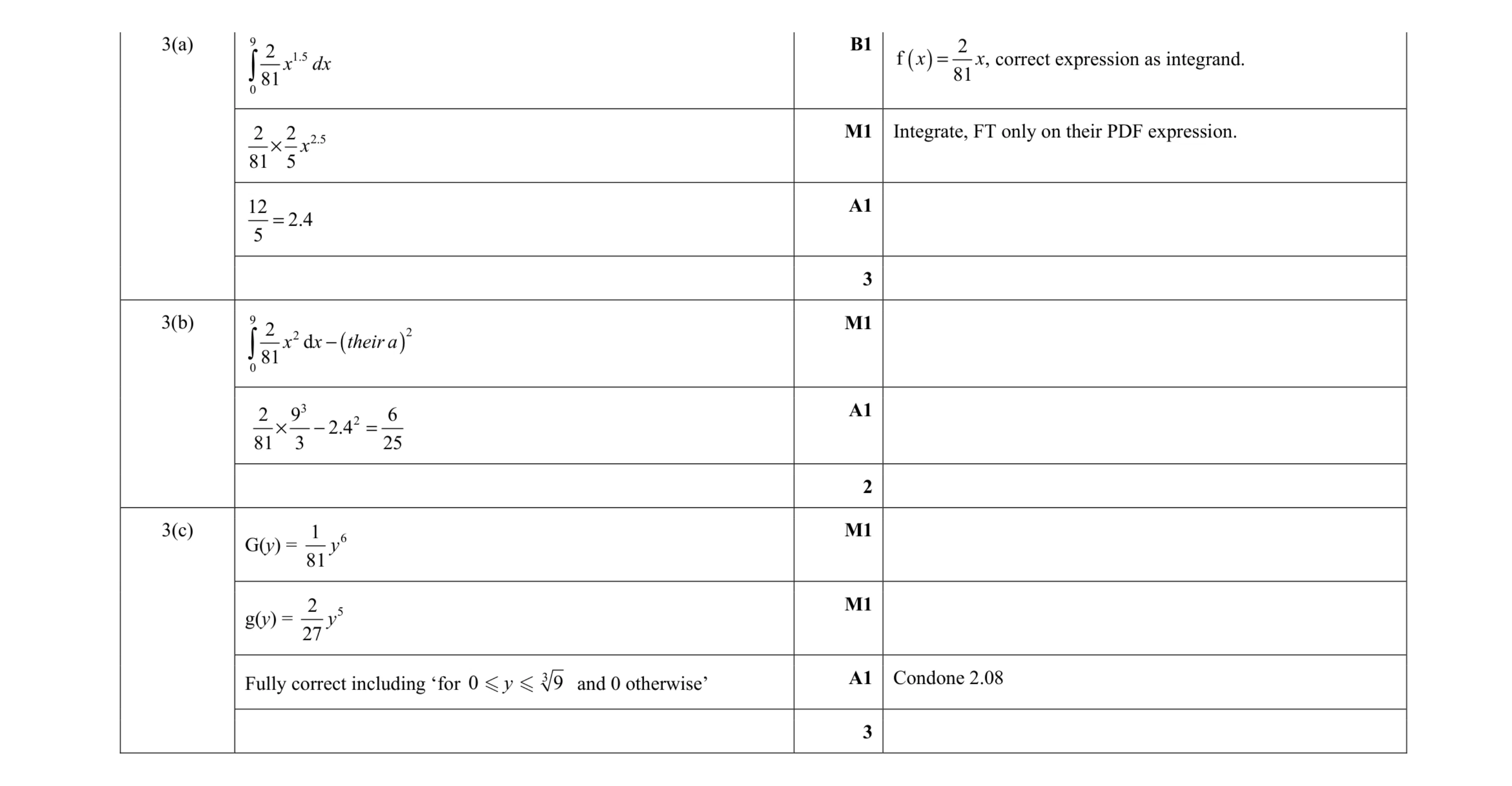 8
8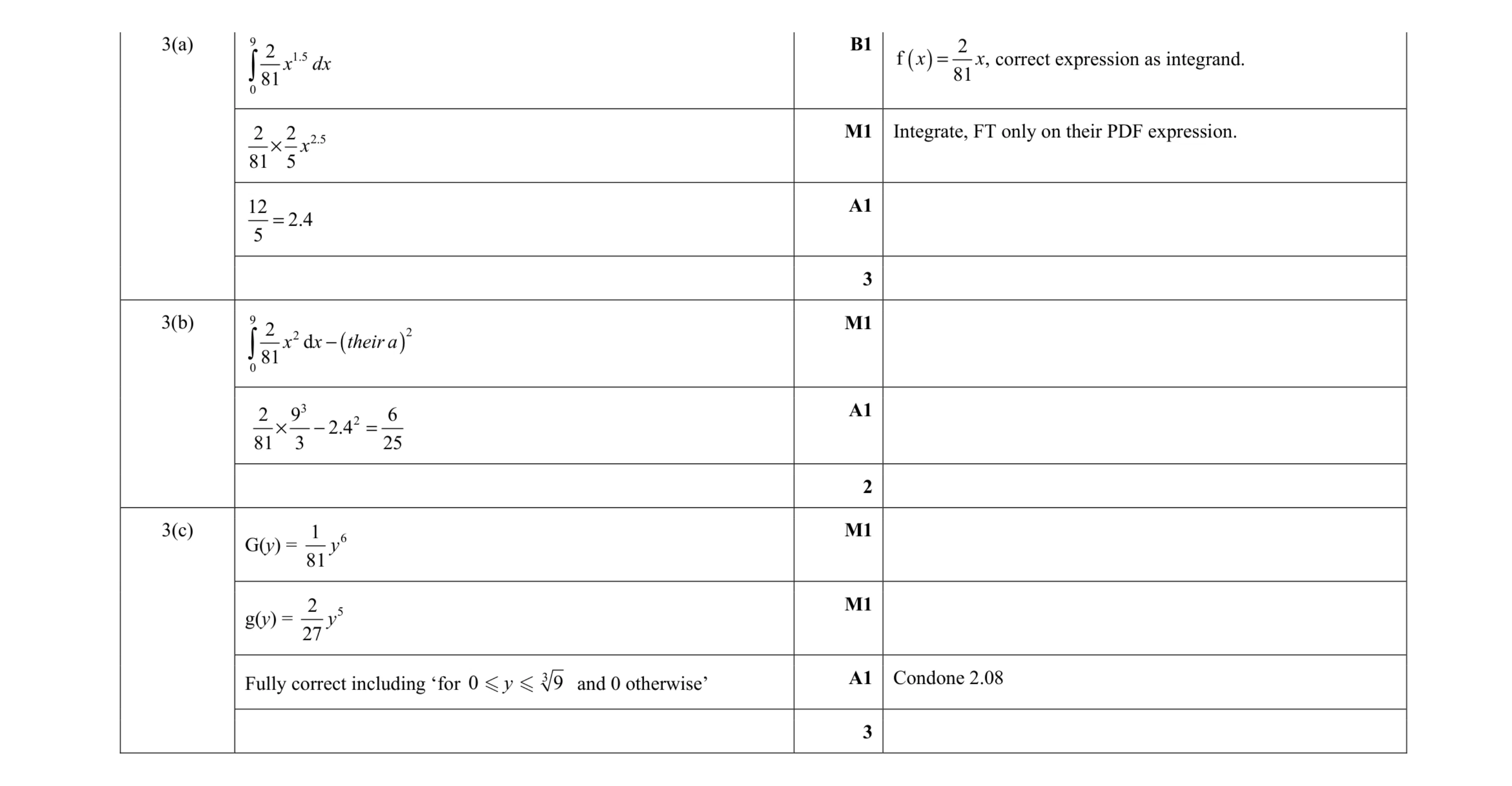 8
8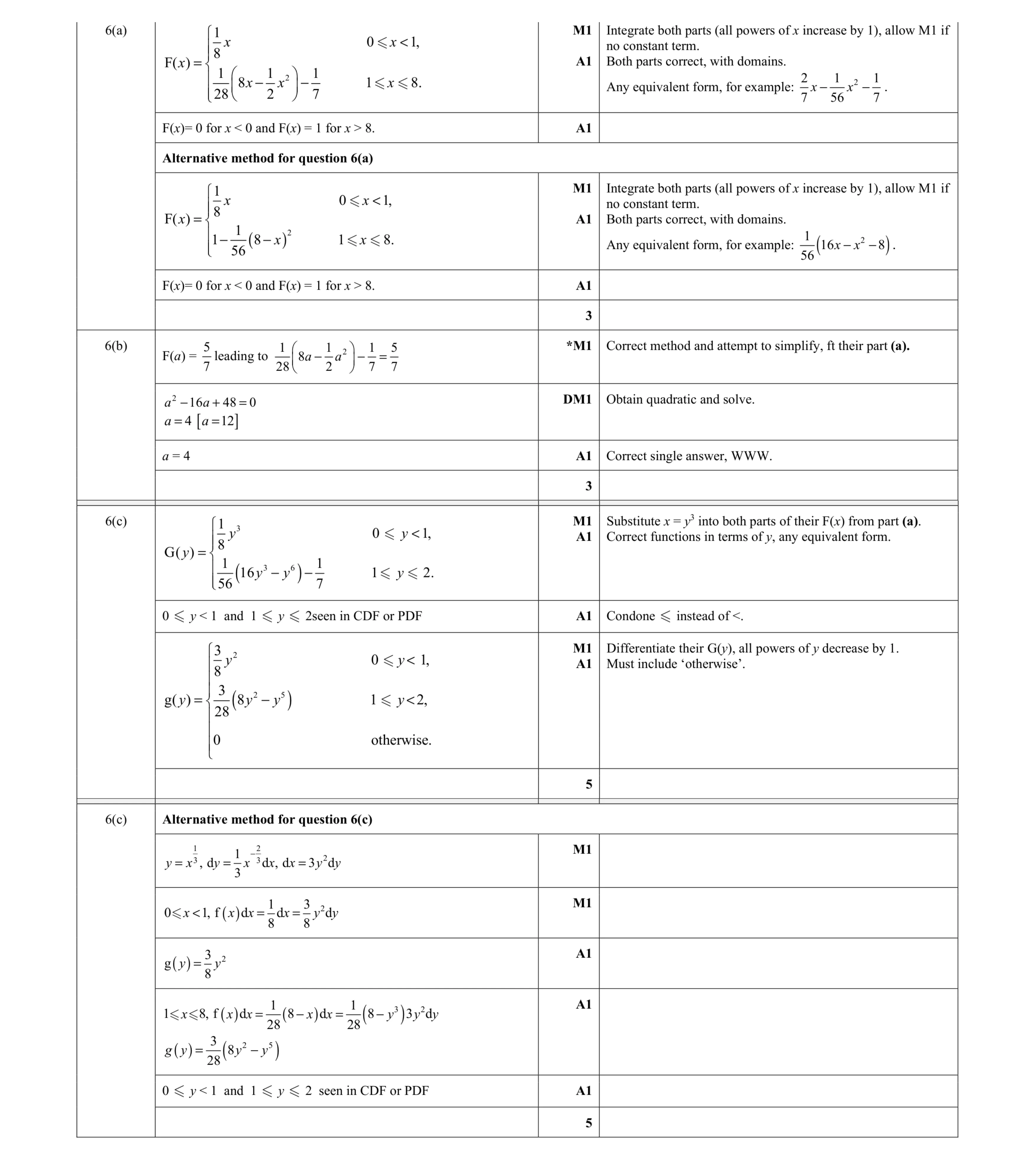 11
11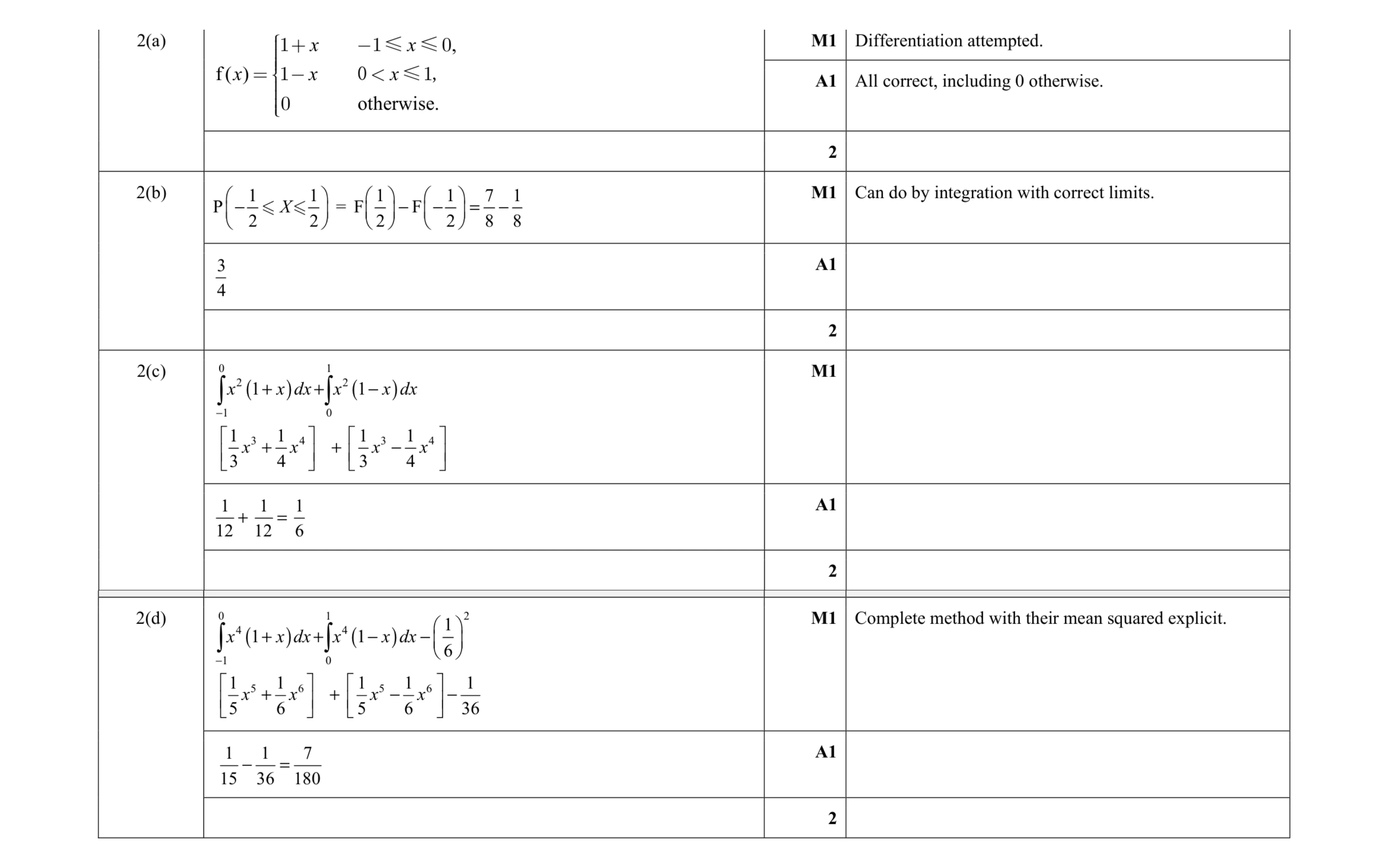 8
8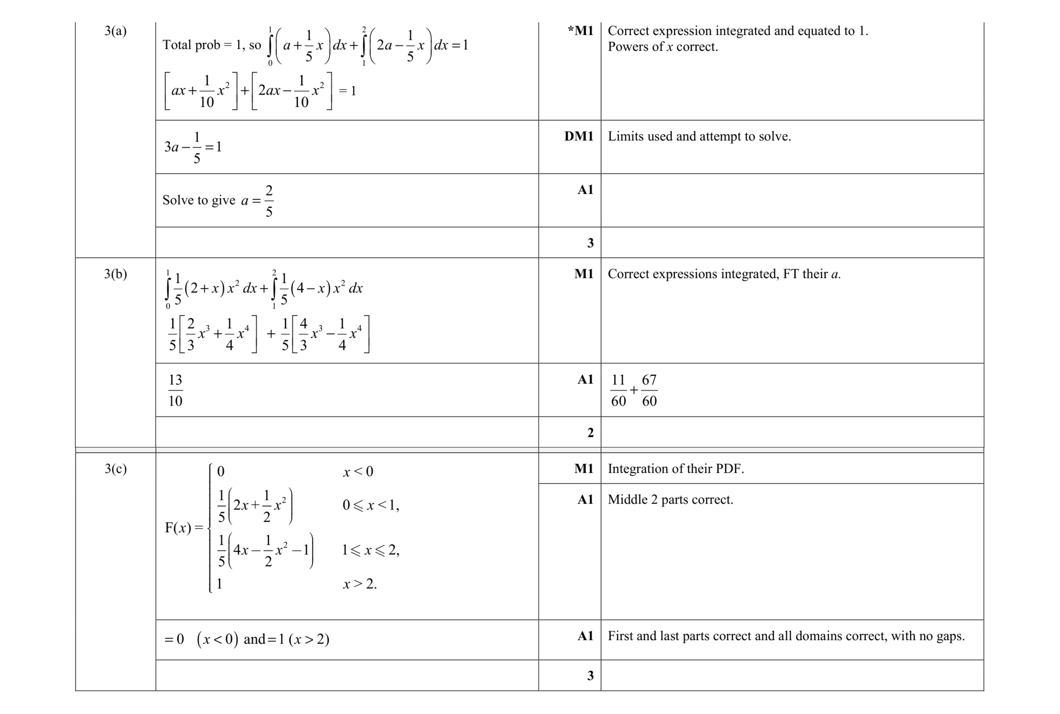 8
8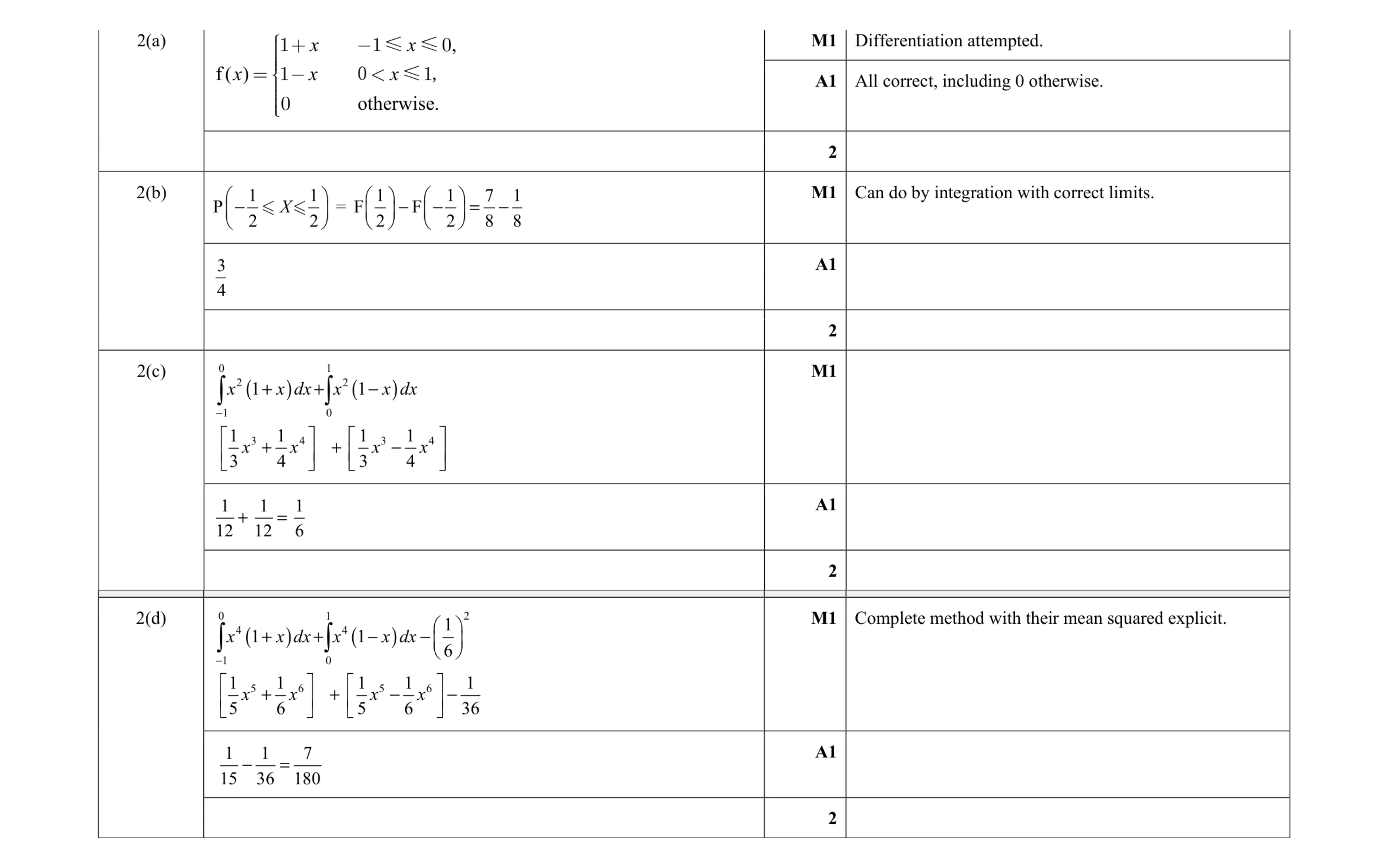 8
8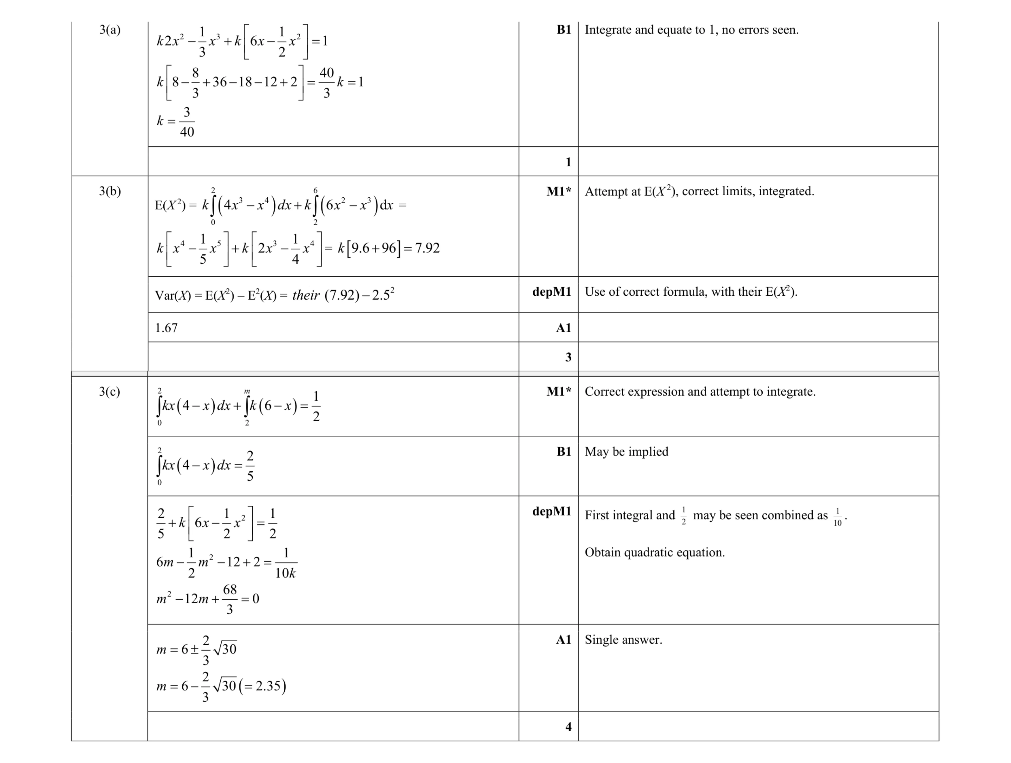 8
8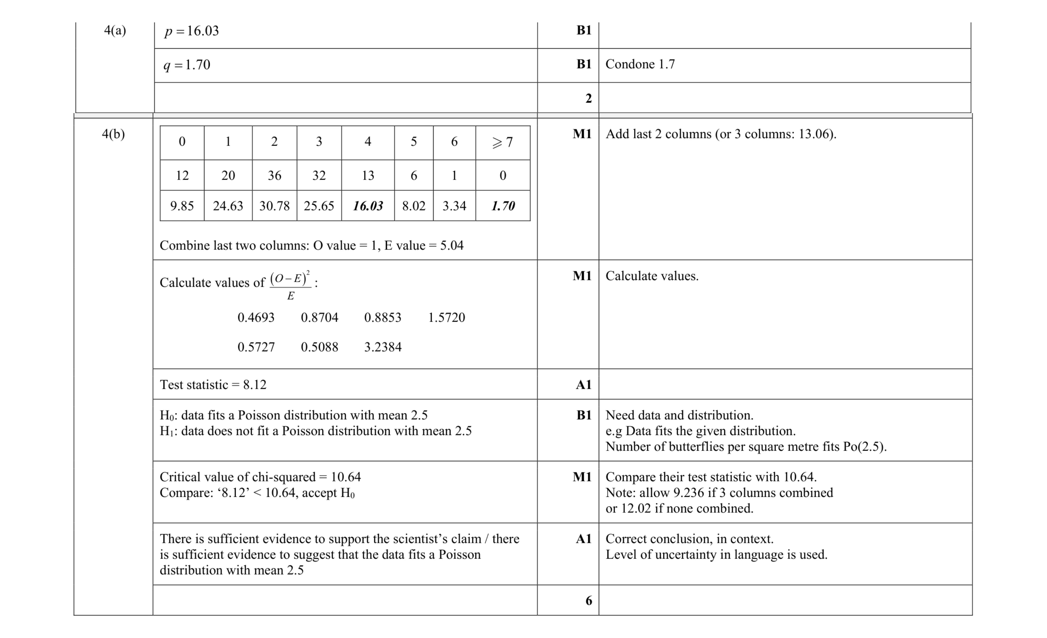 8
8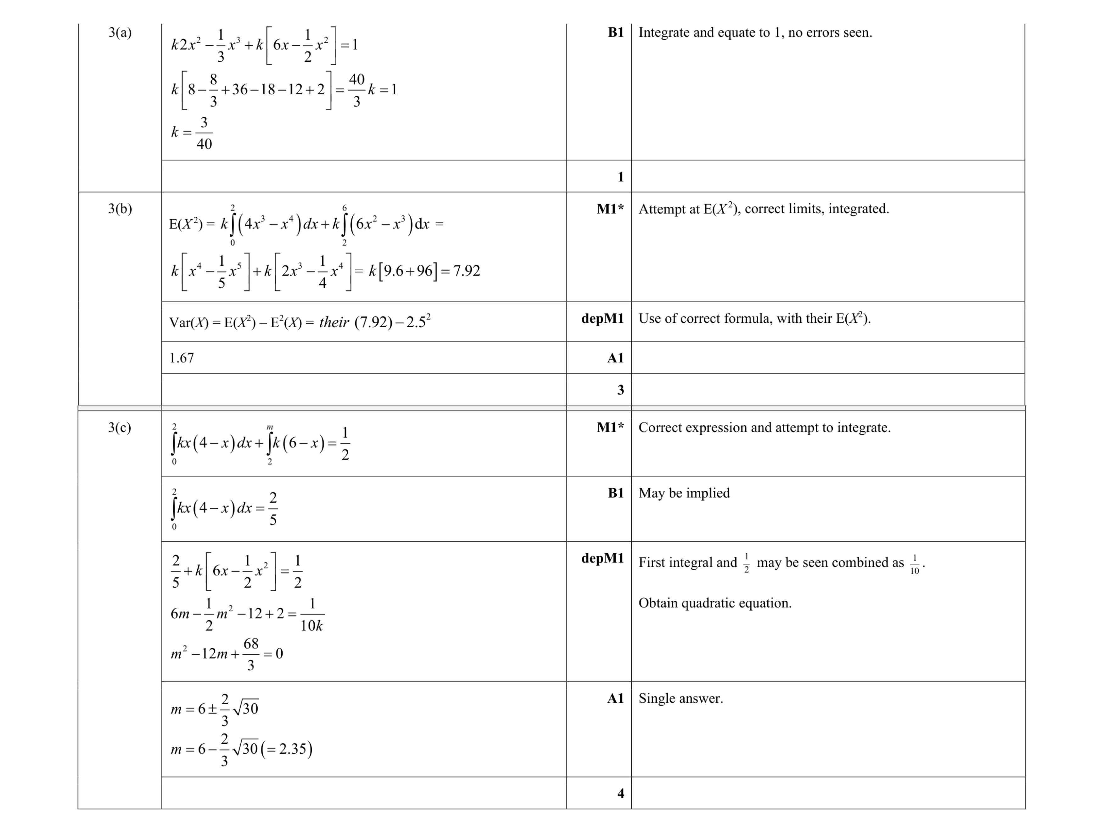 8
8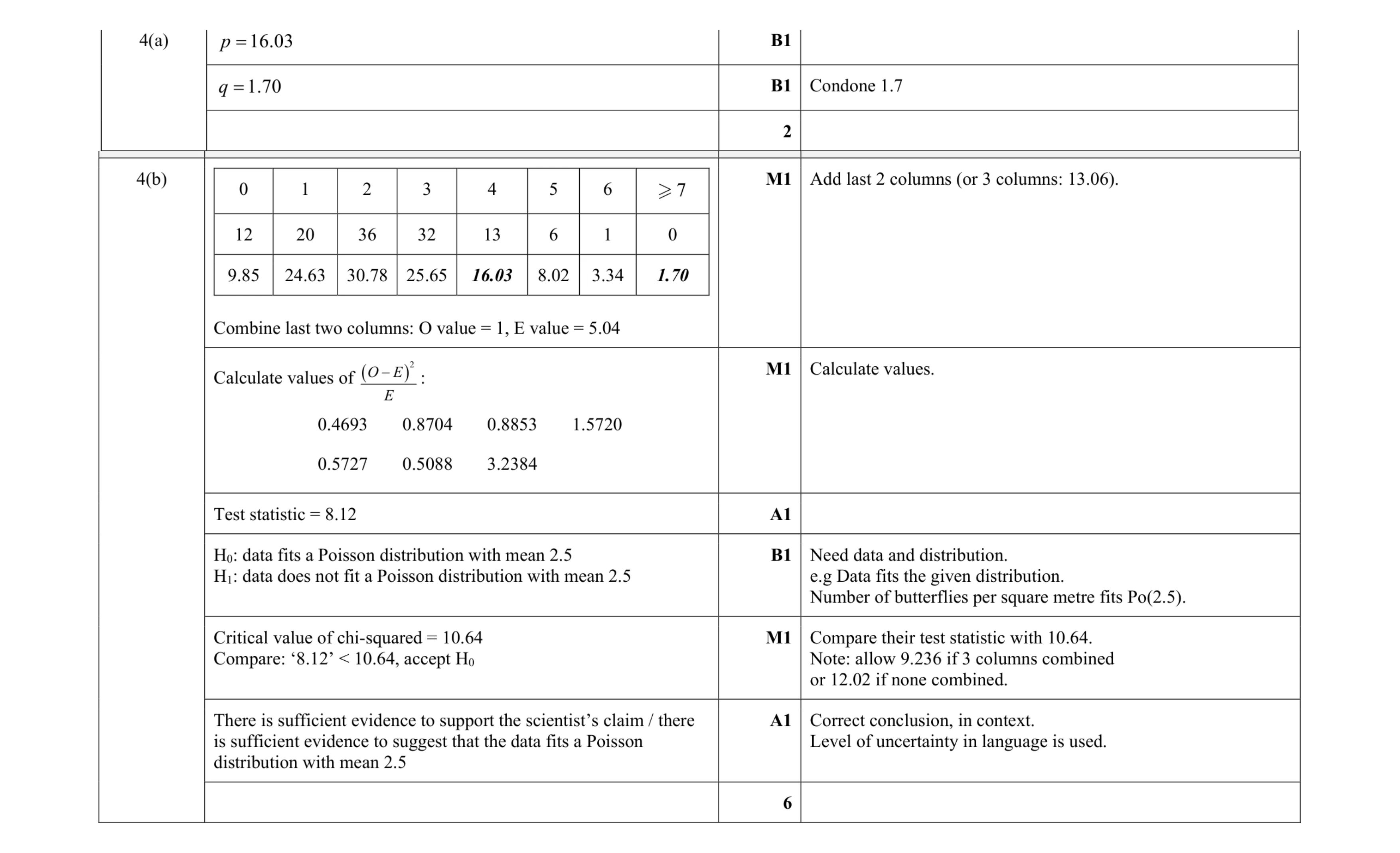 8
8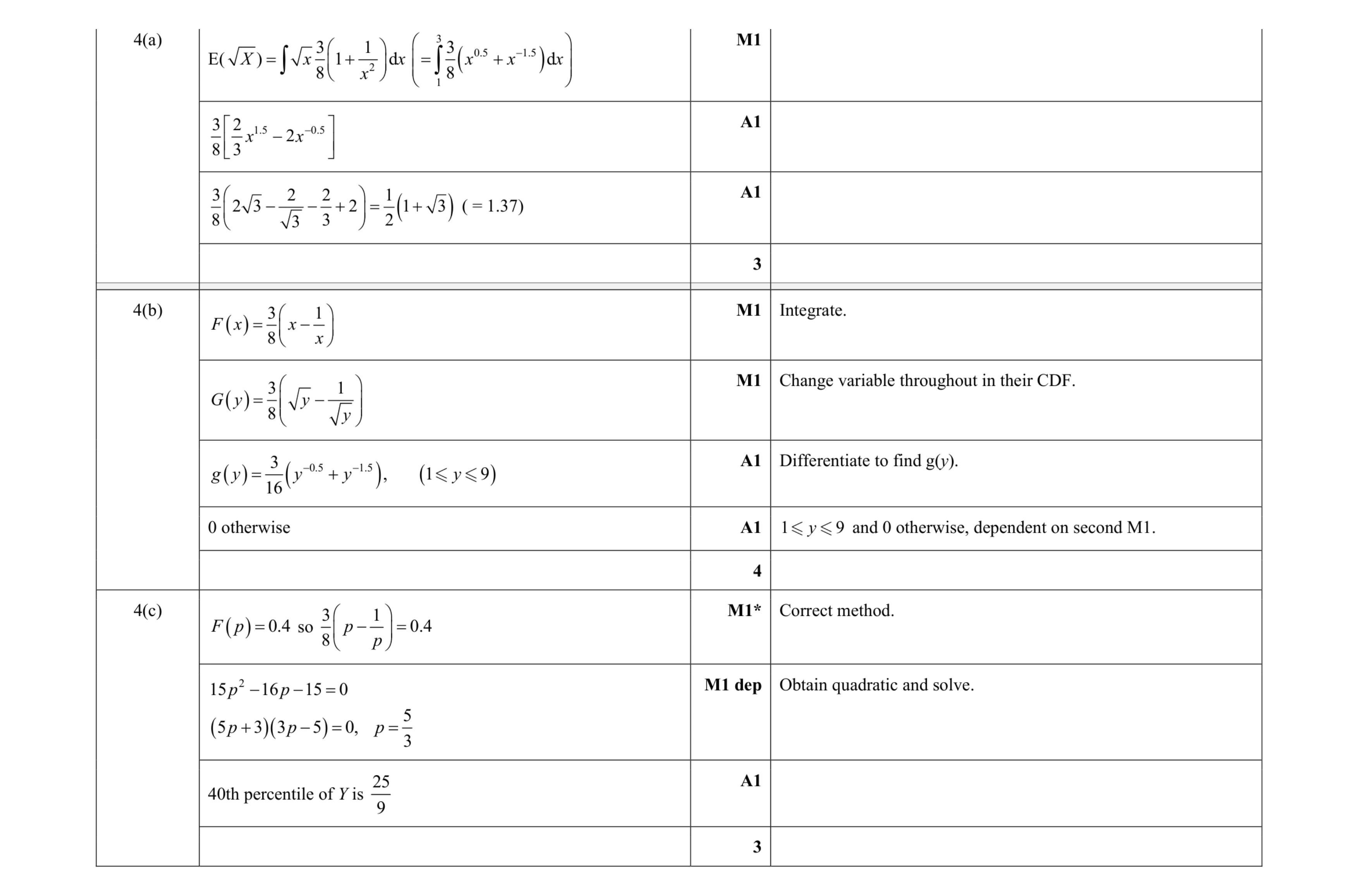 10
10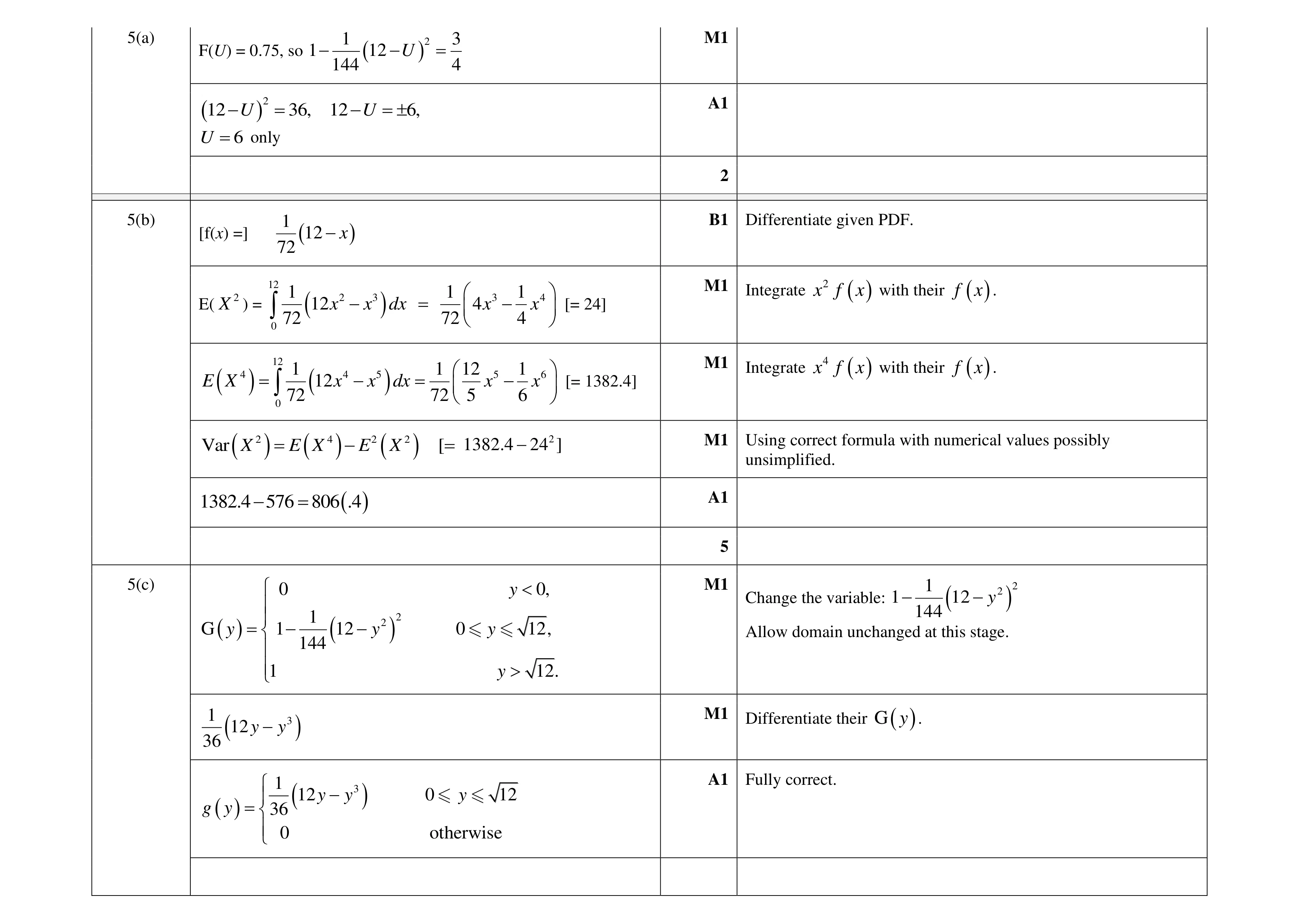 10
10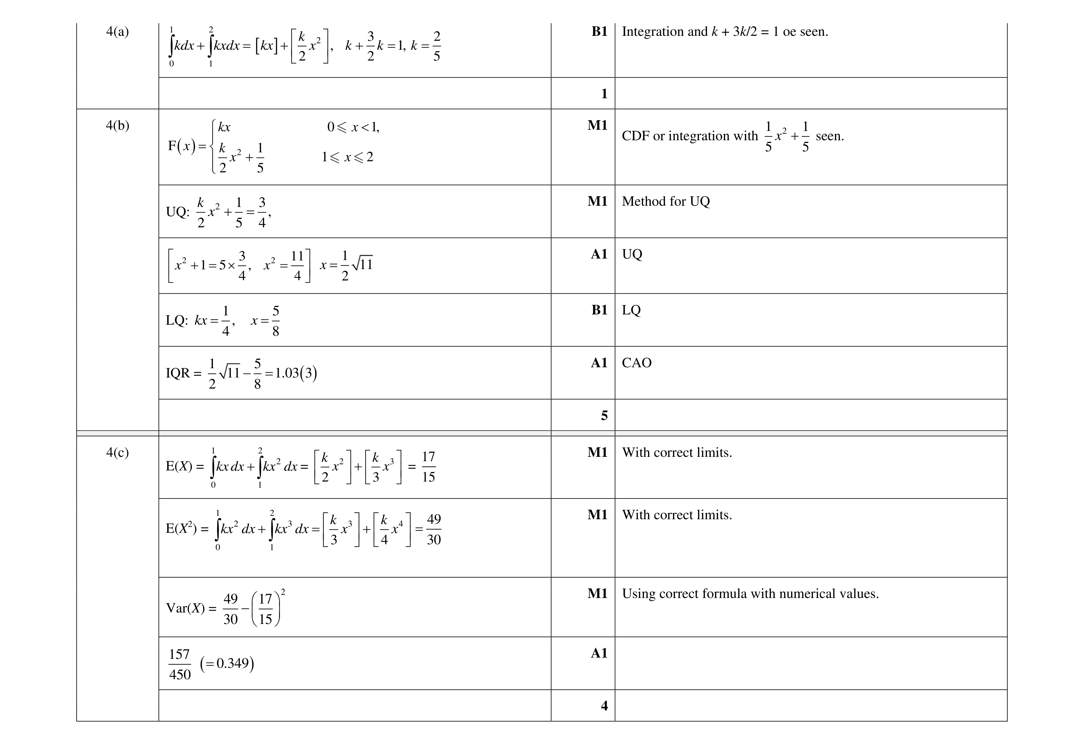 10
10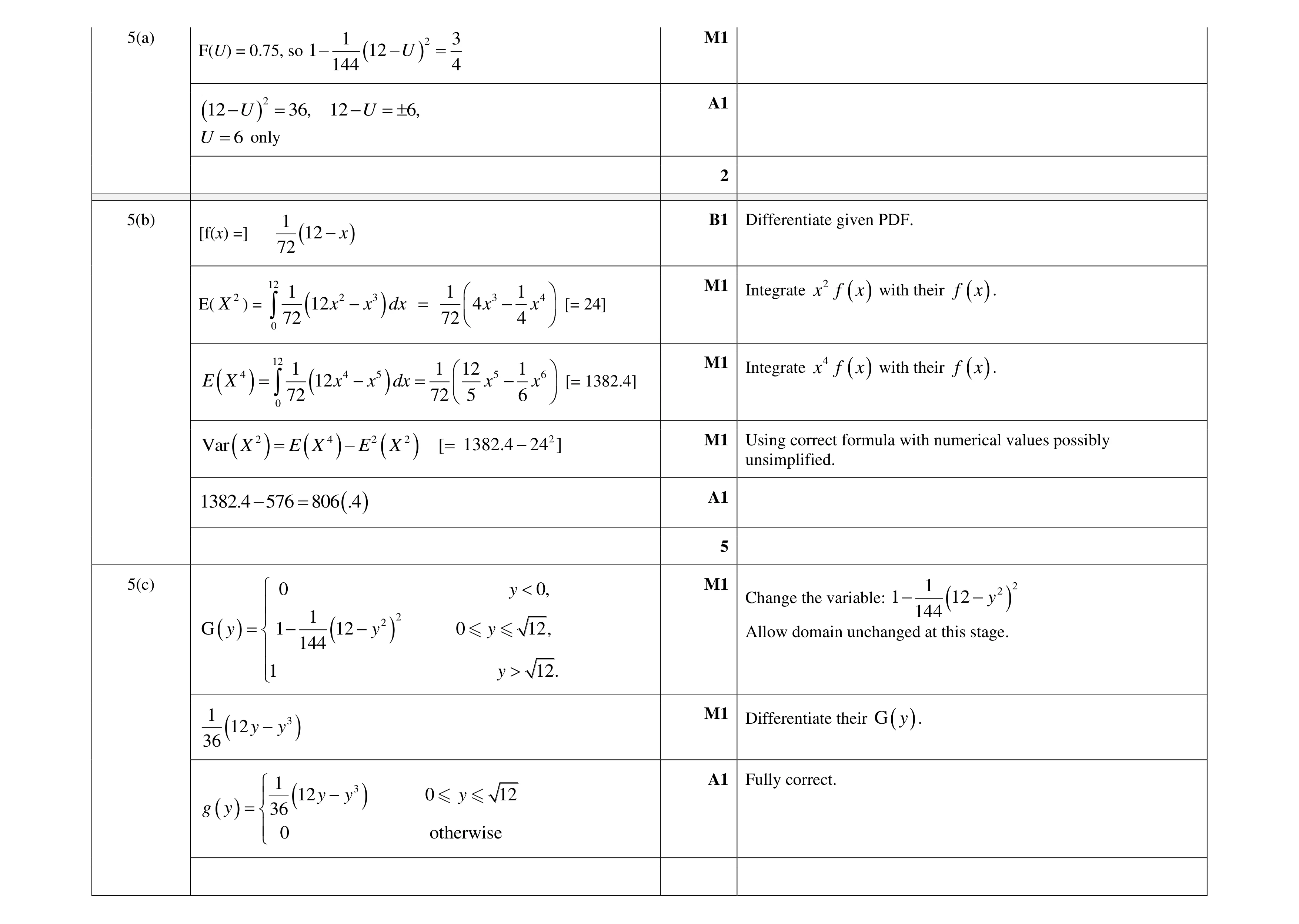 10
10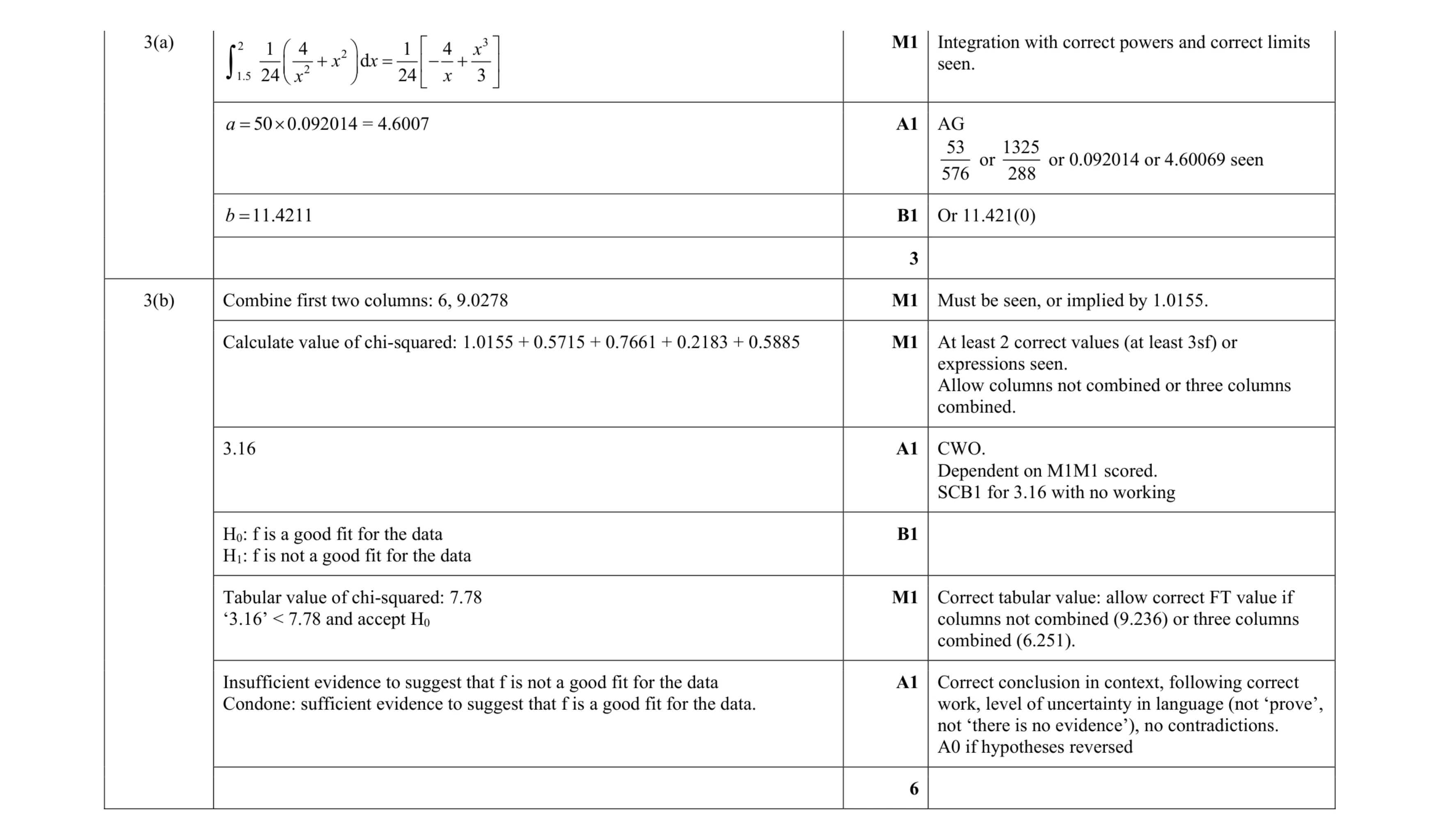 9
9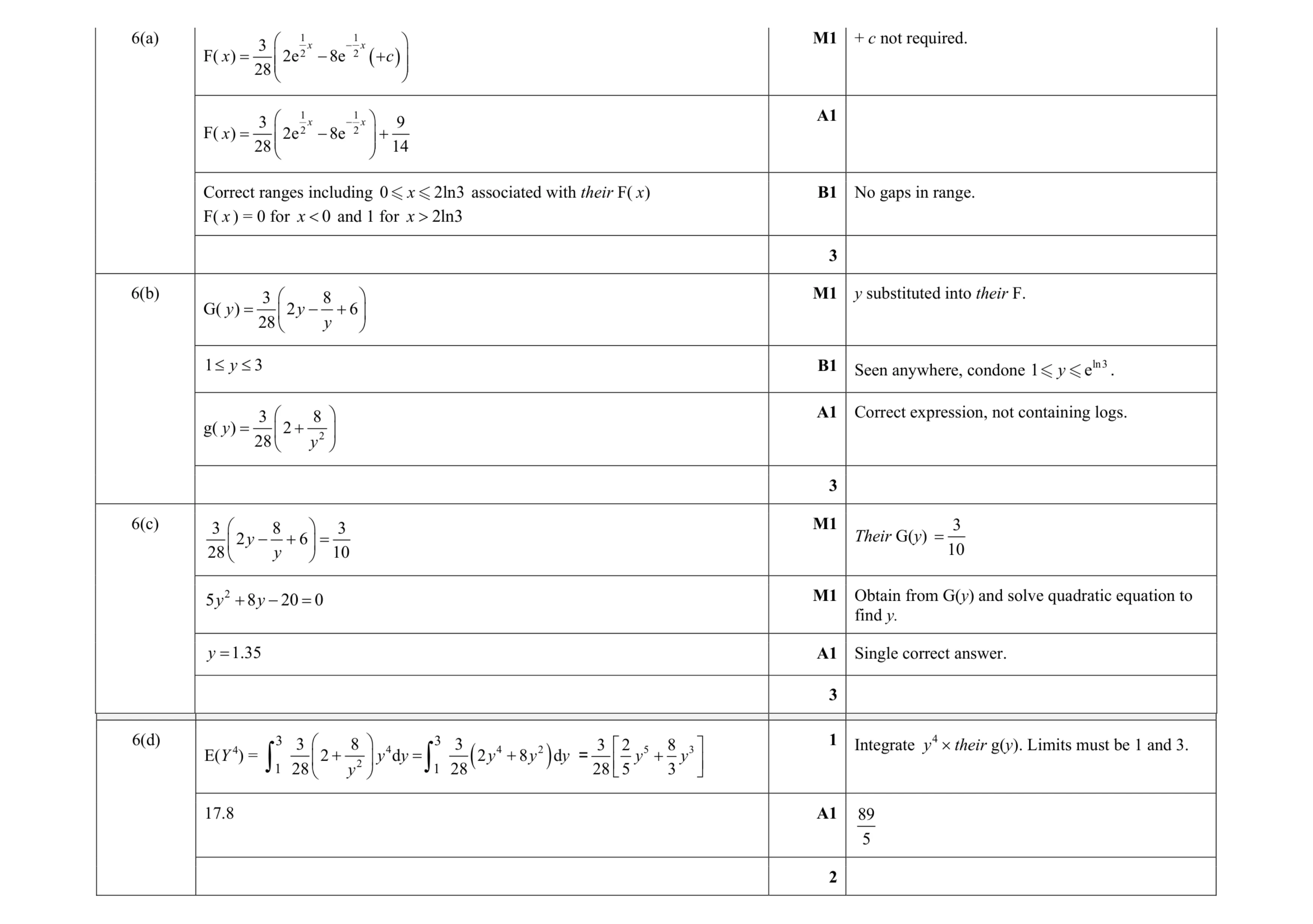 11
11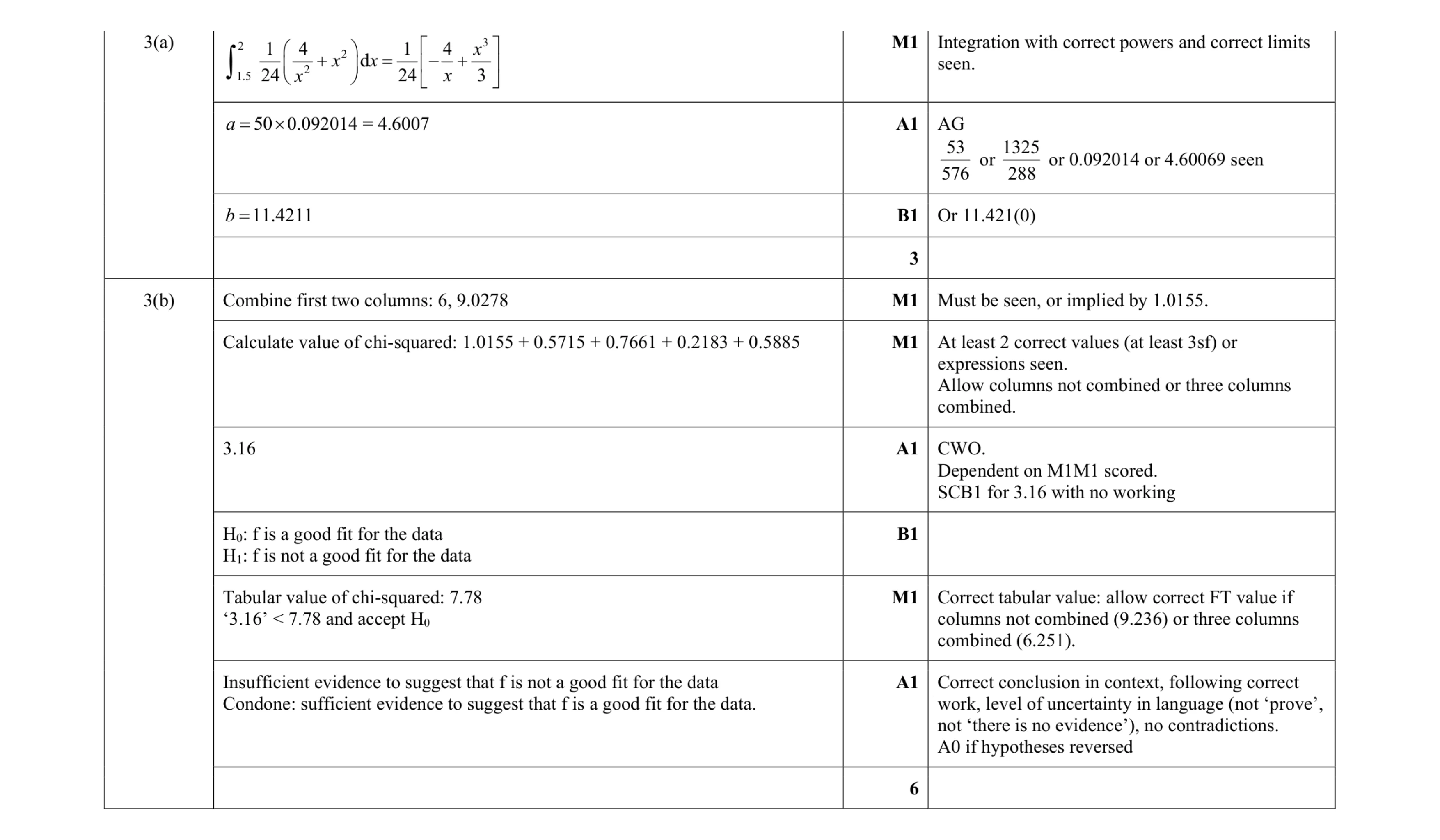 9
9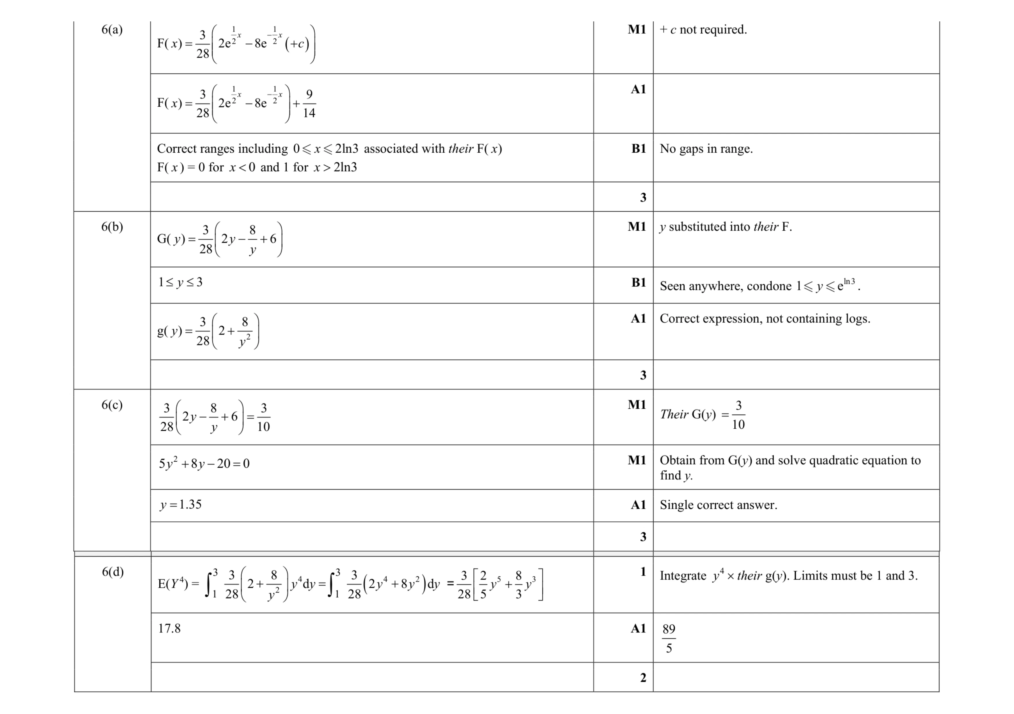 11
11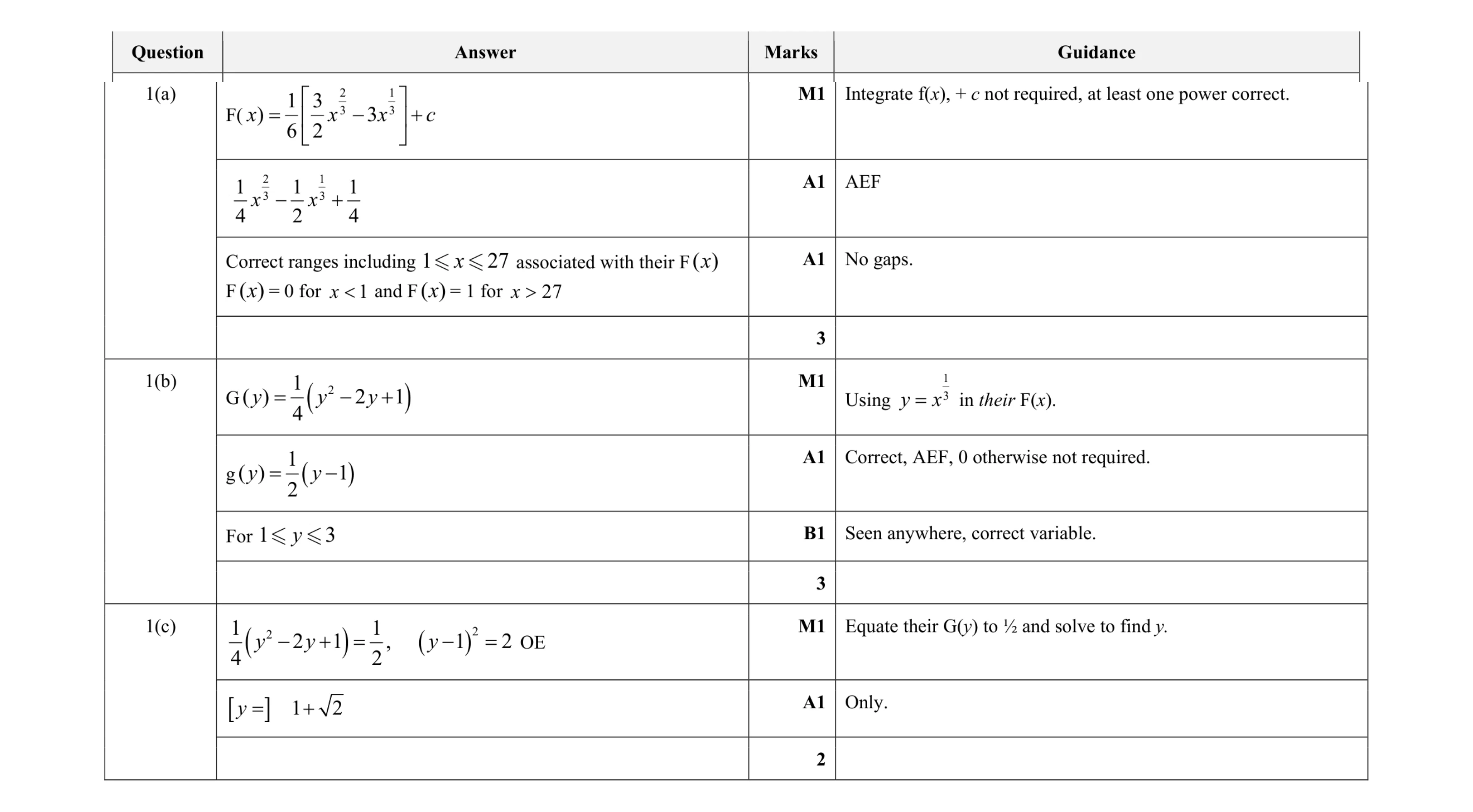 8
8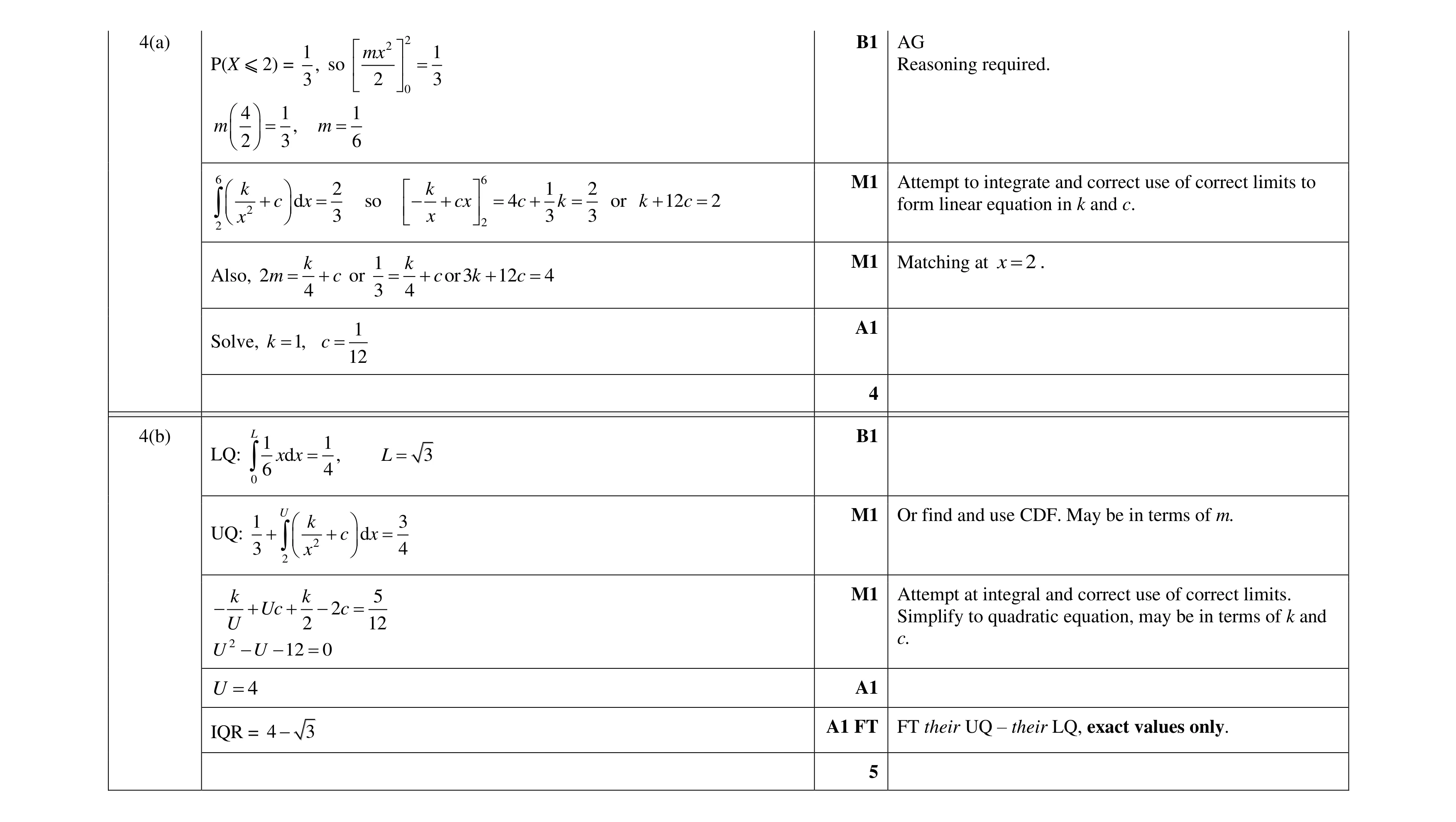 9
9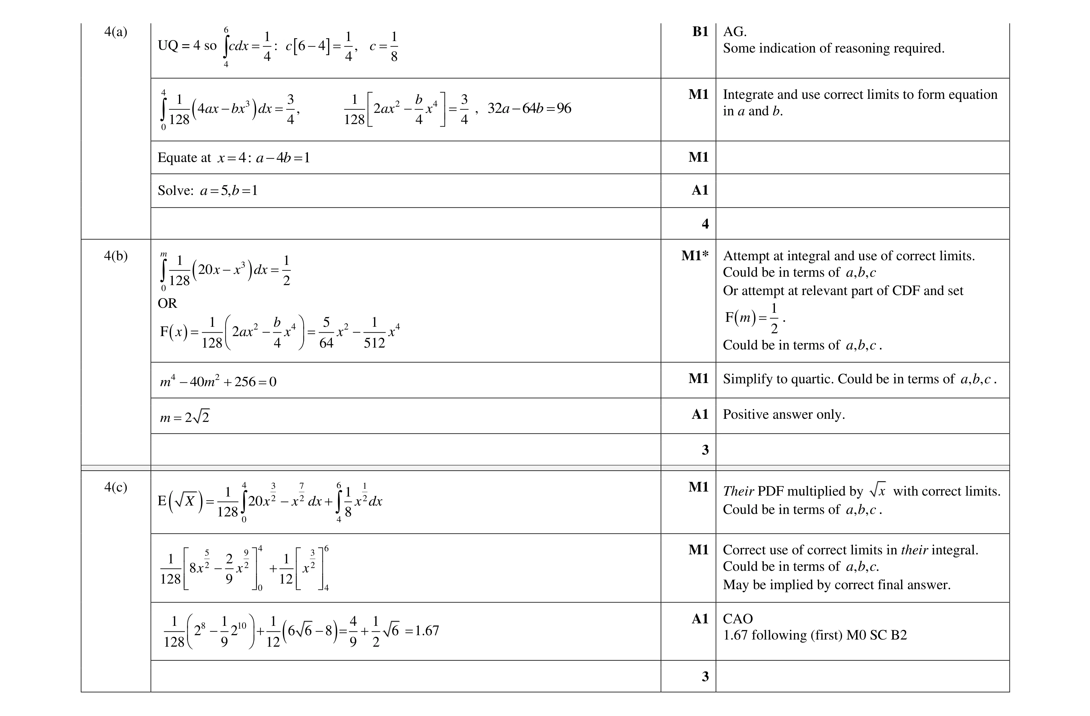 10
10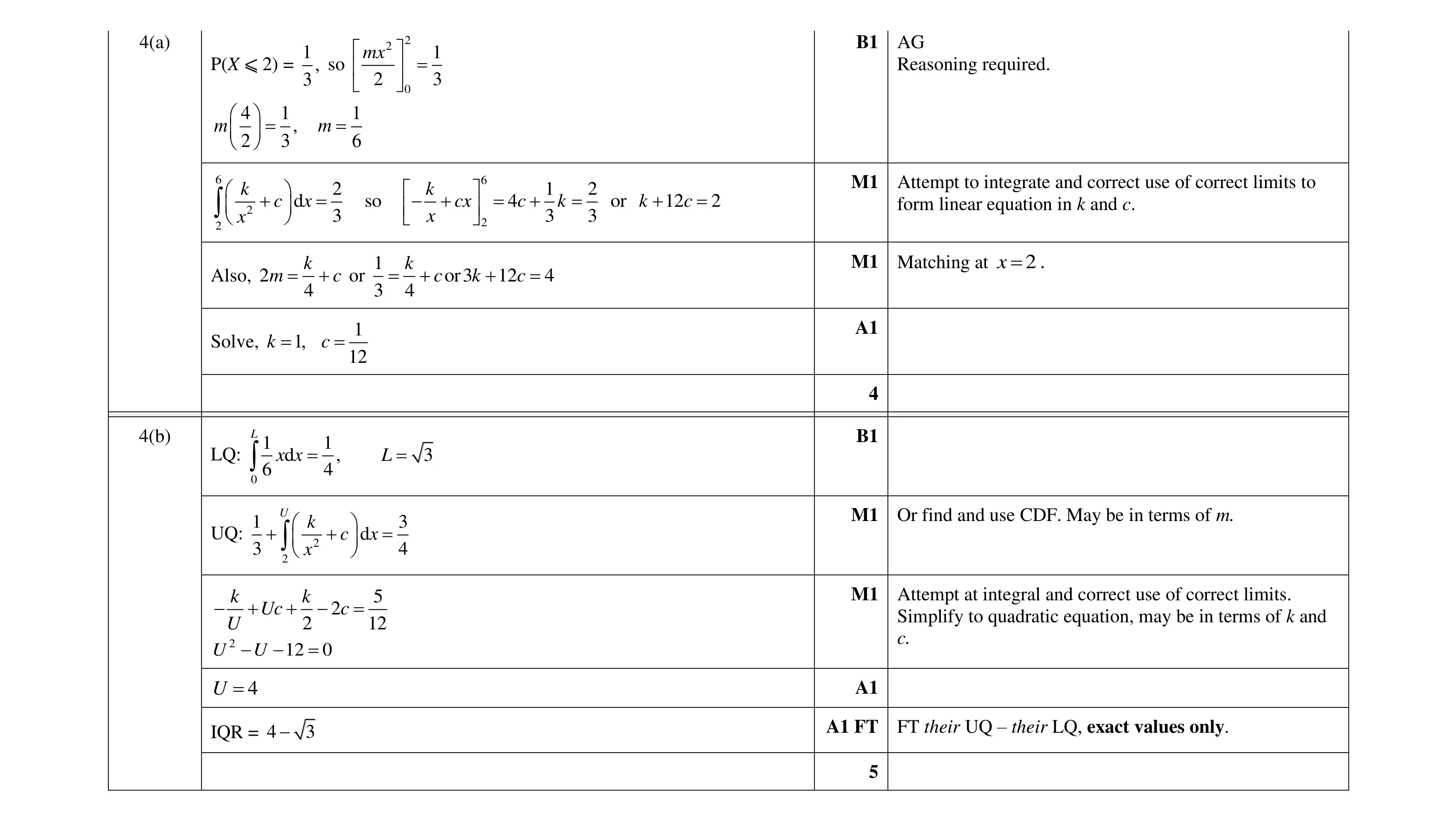 9
9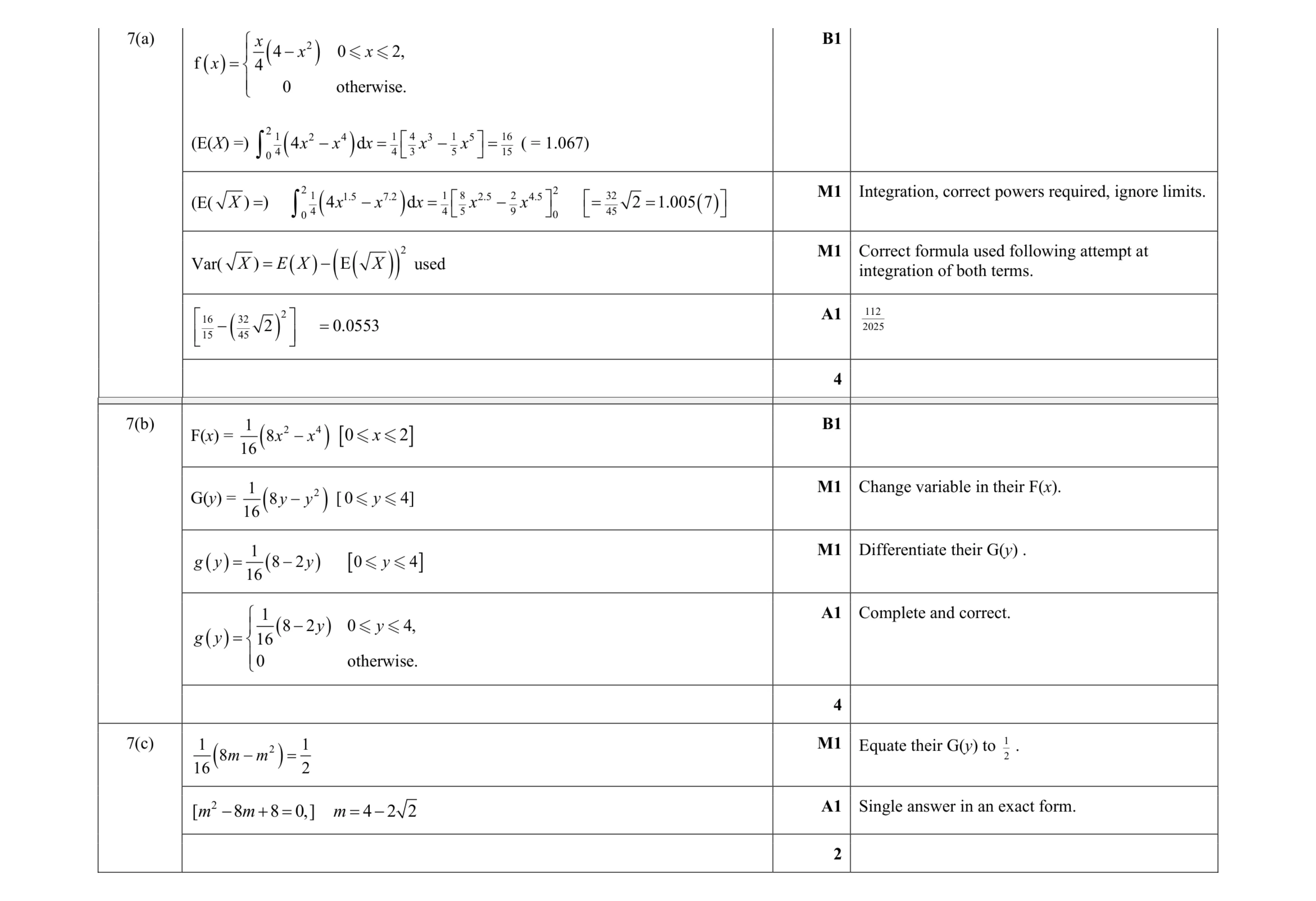 10
10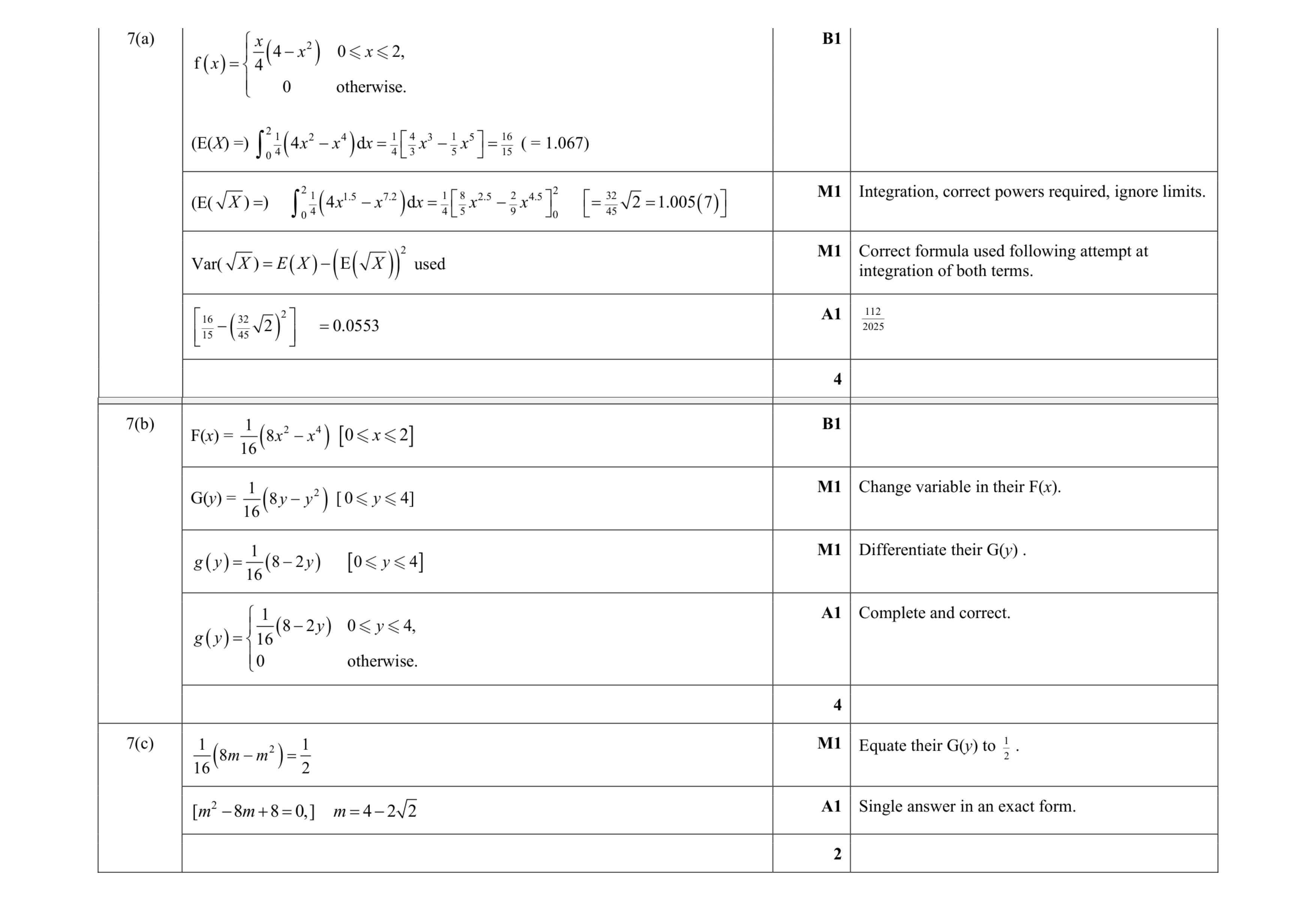 10
10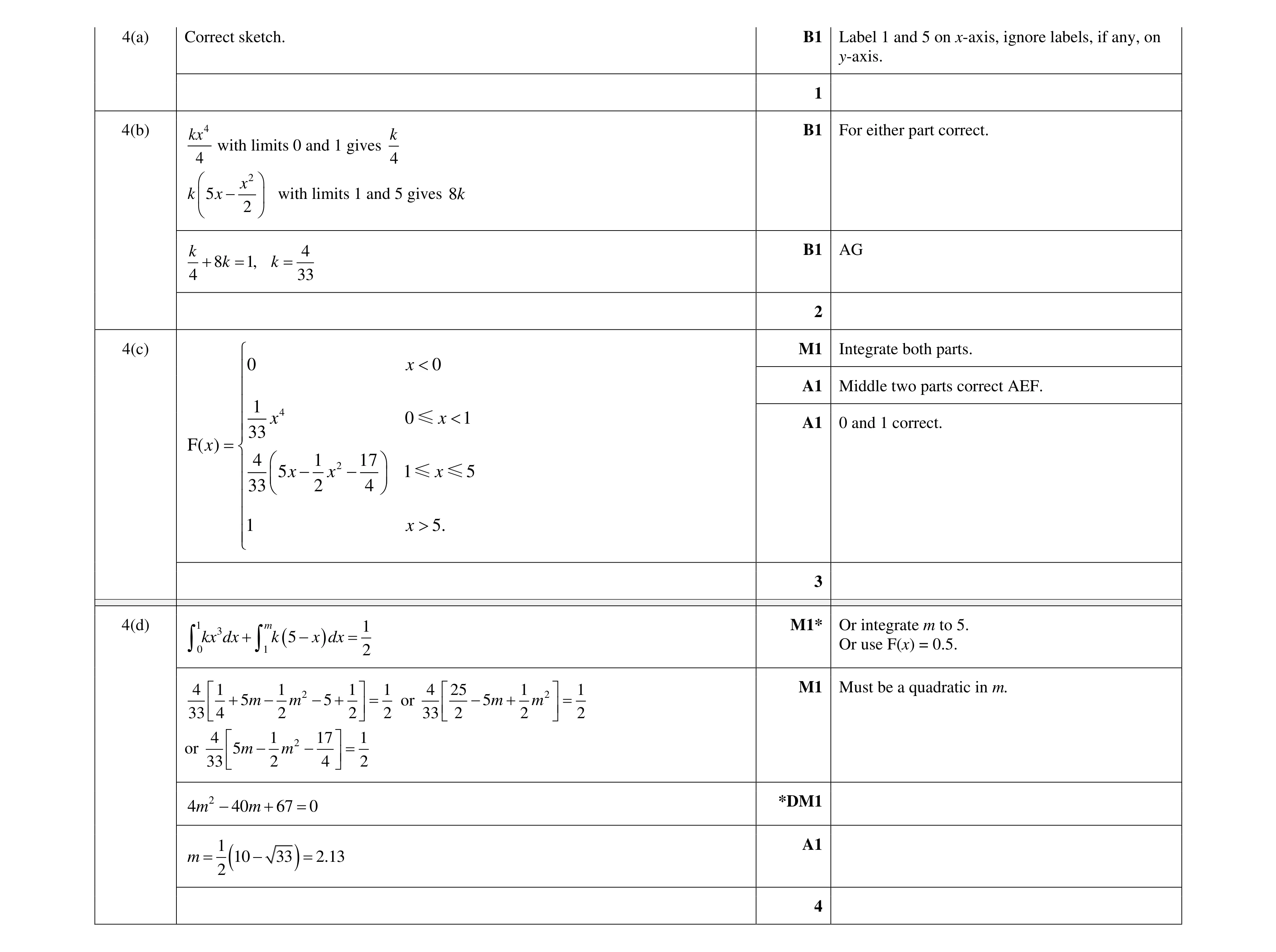 10
10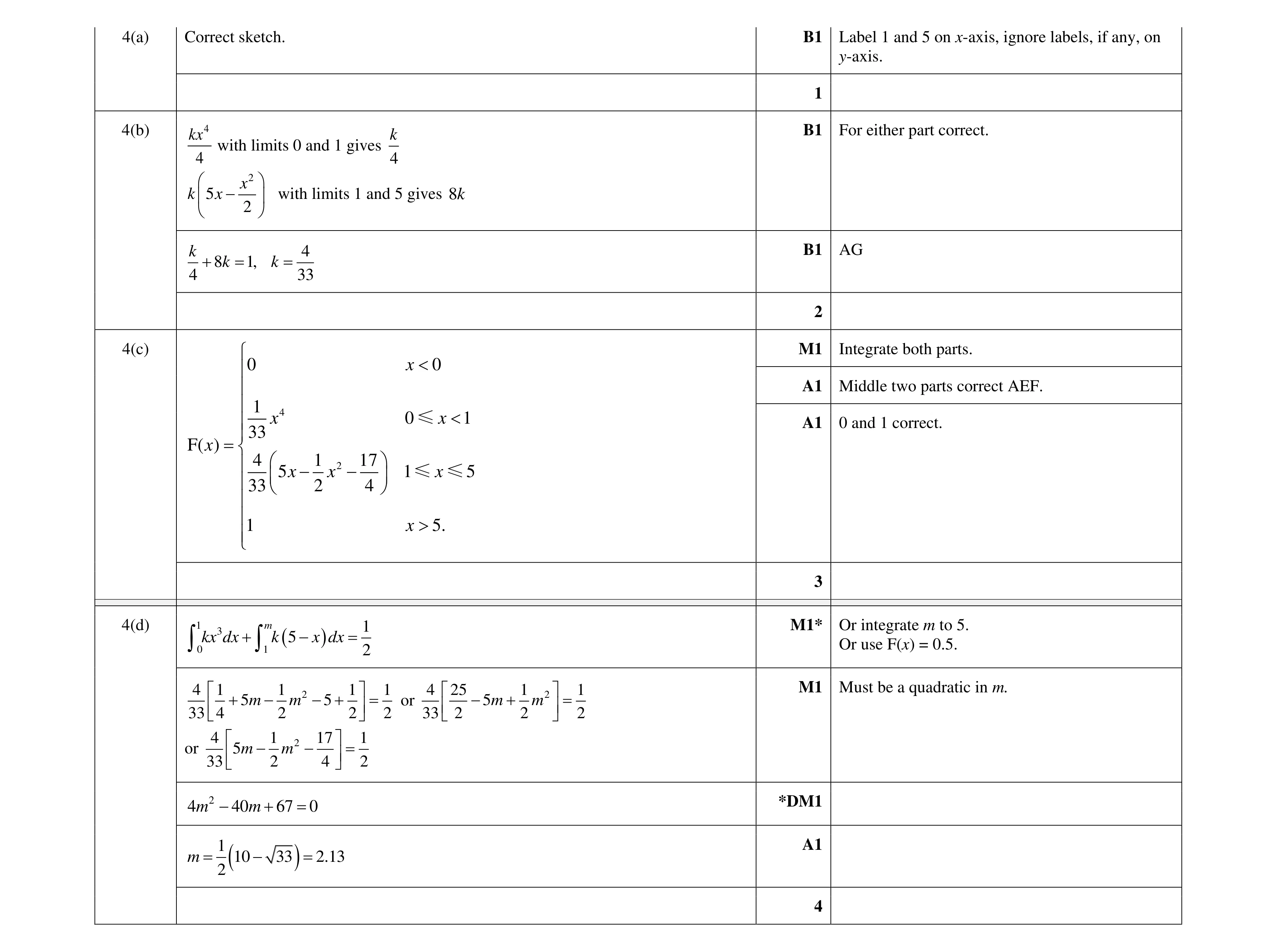 10
10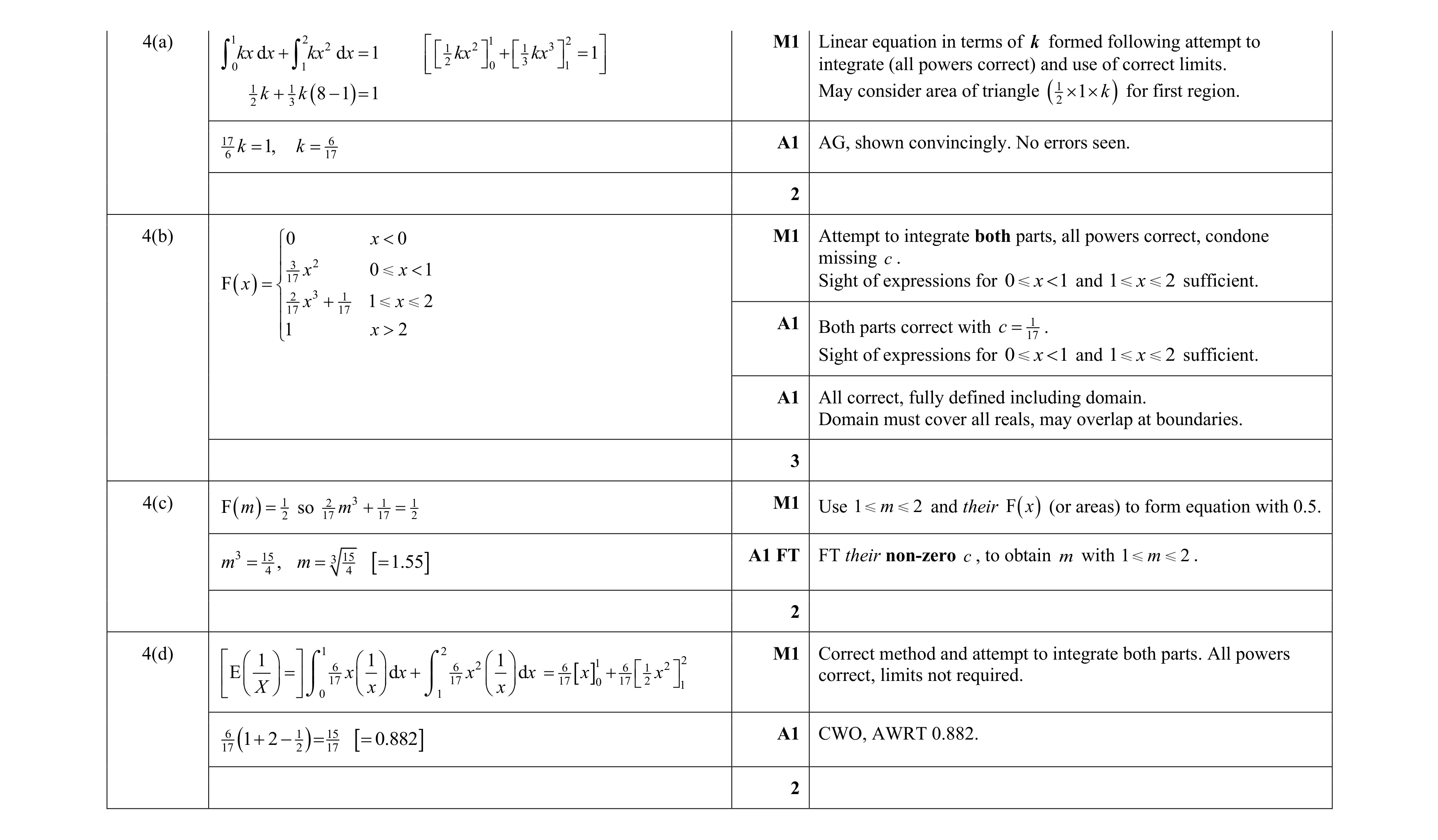 9
9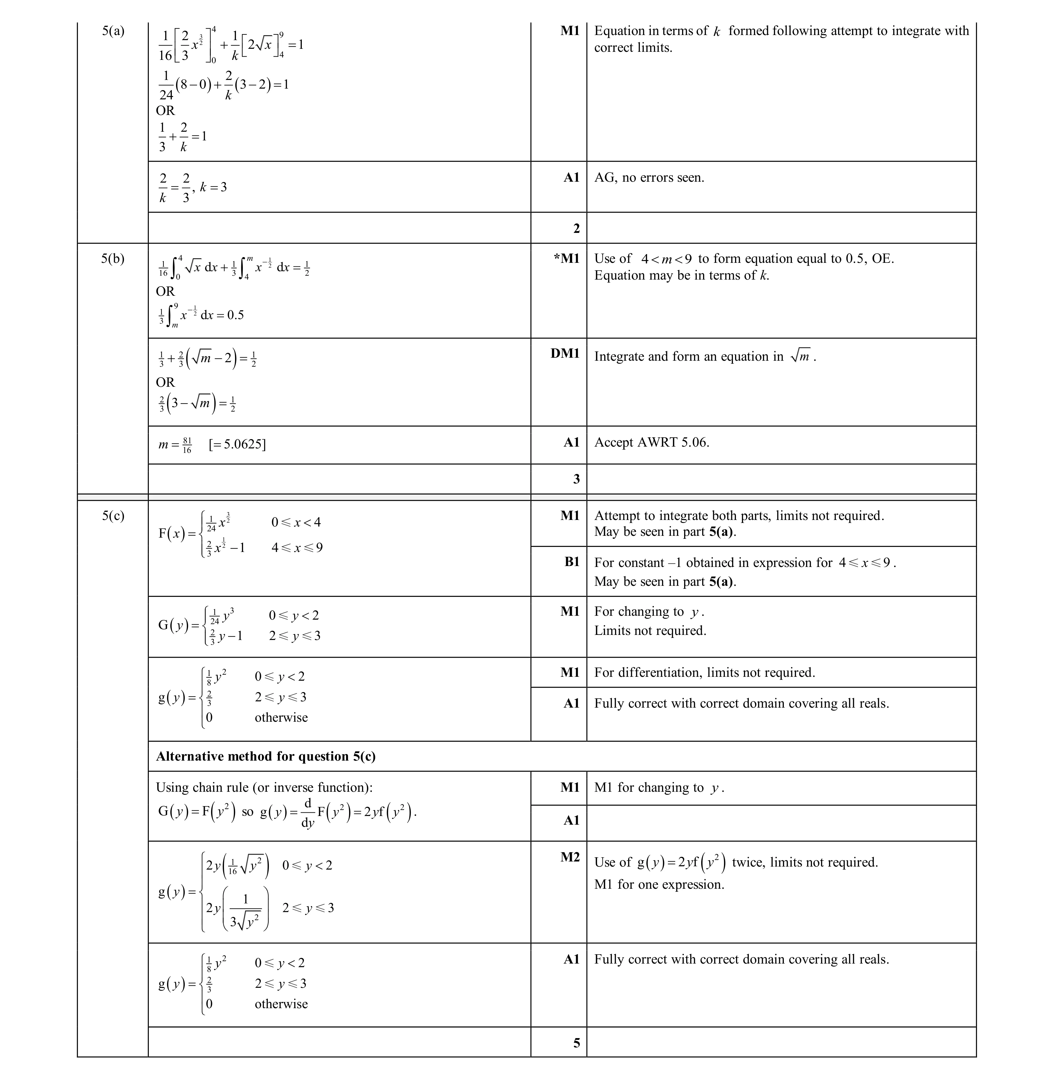 10
10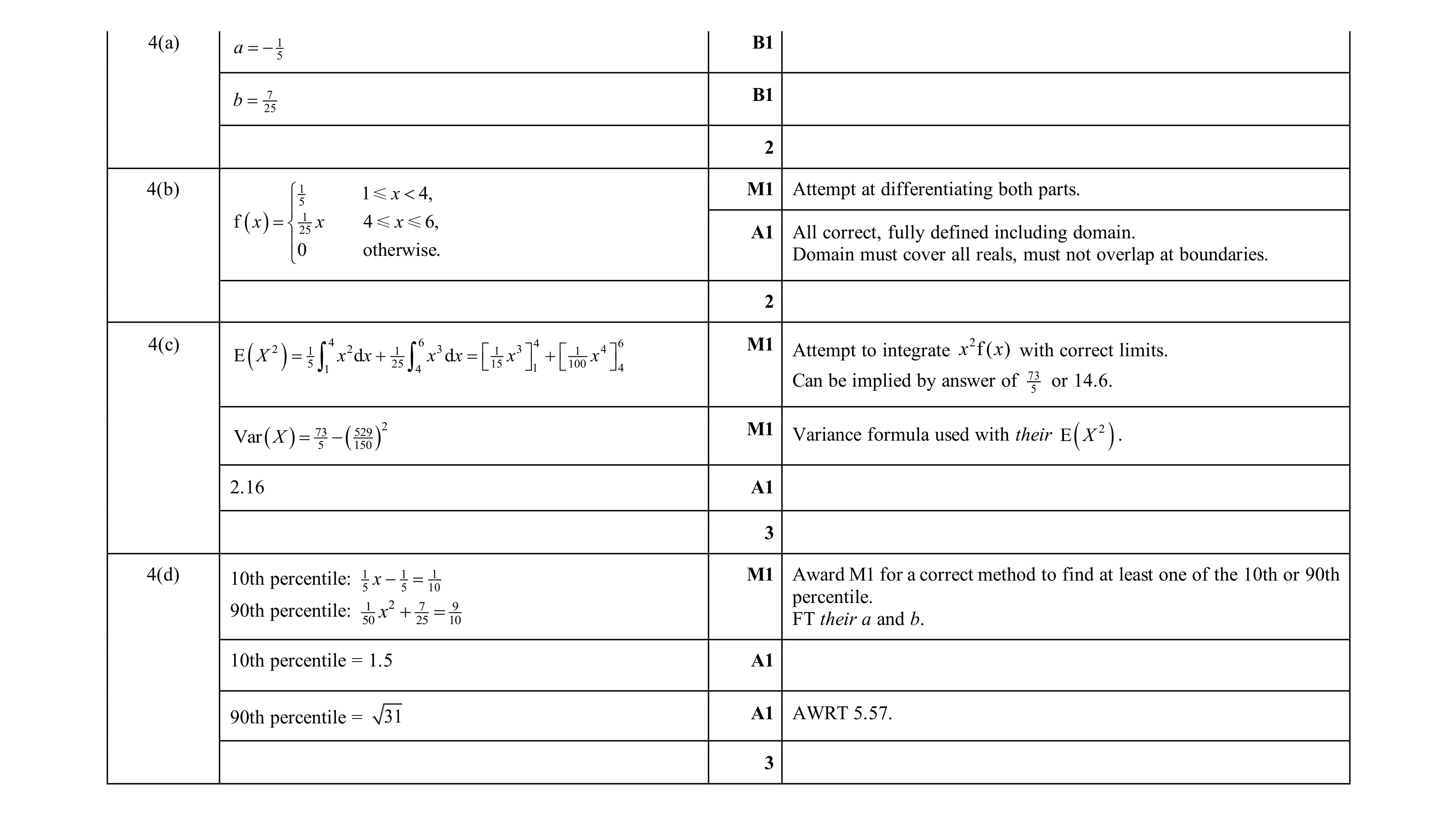 10
10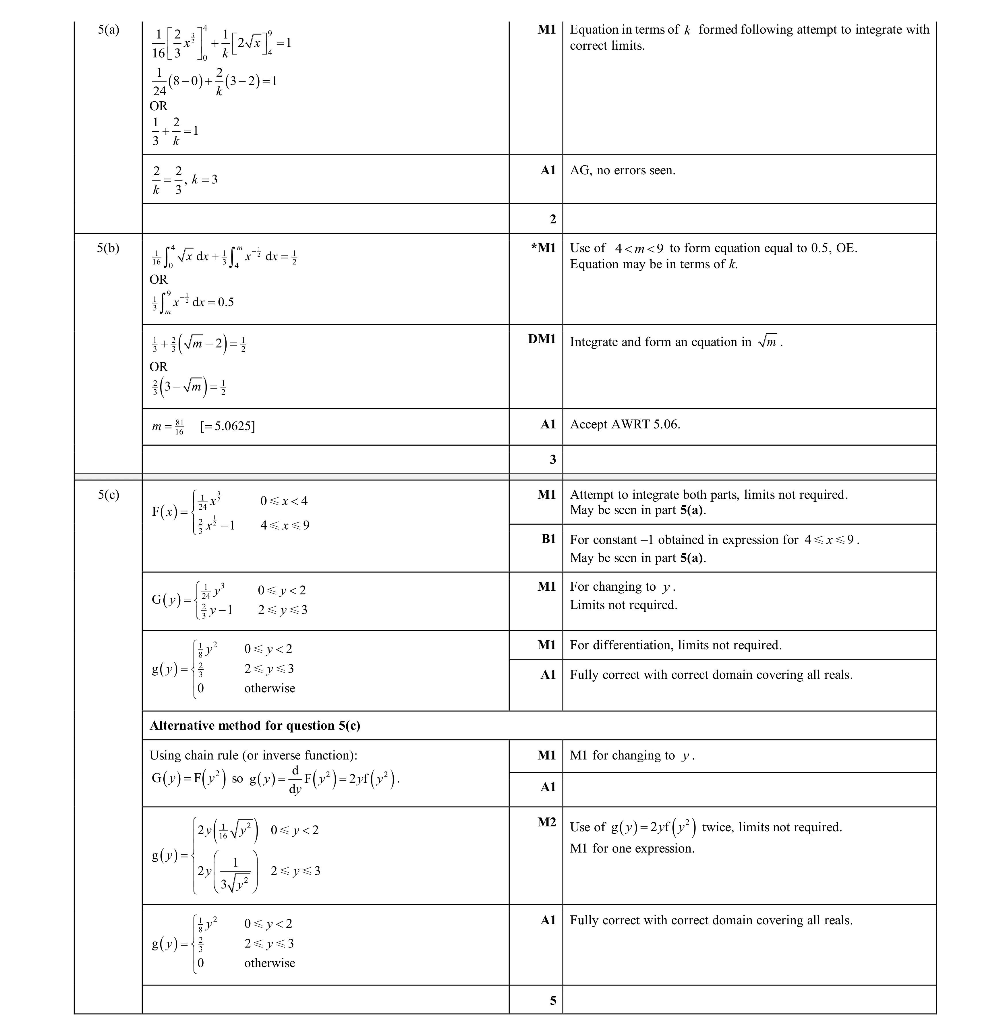 10
10