Cambridge A Level Physics 9702 — 2024 May/June Paper 3 · Variant 3

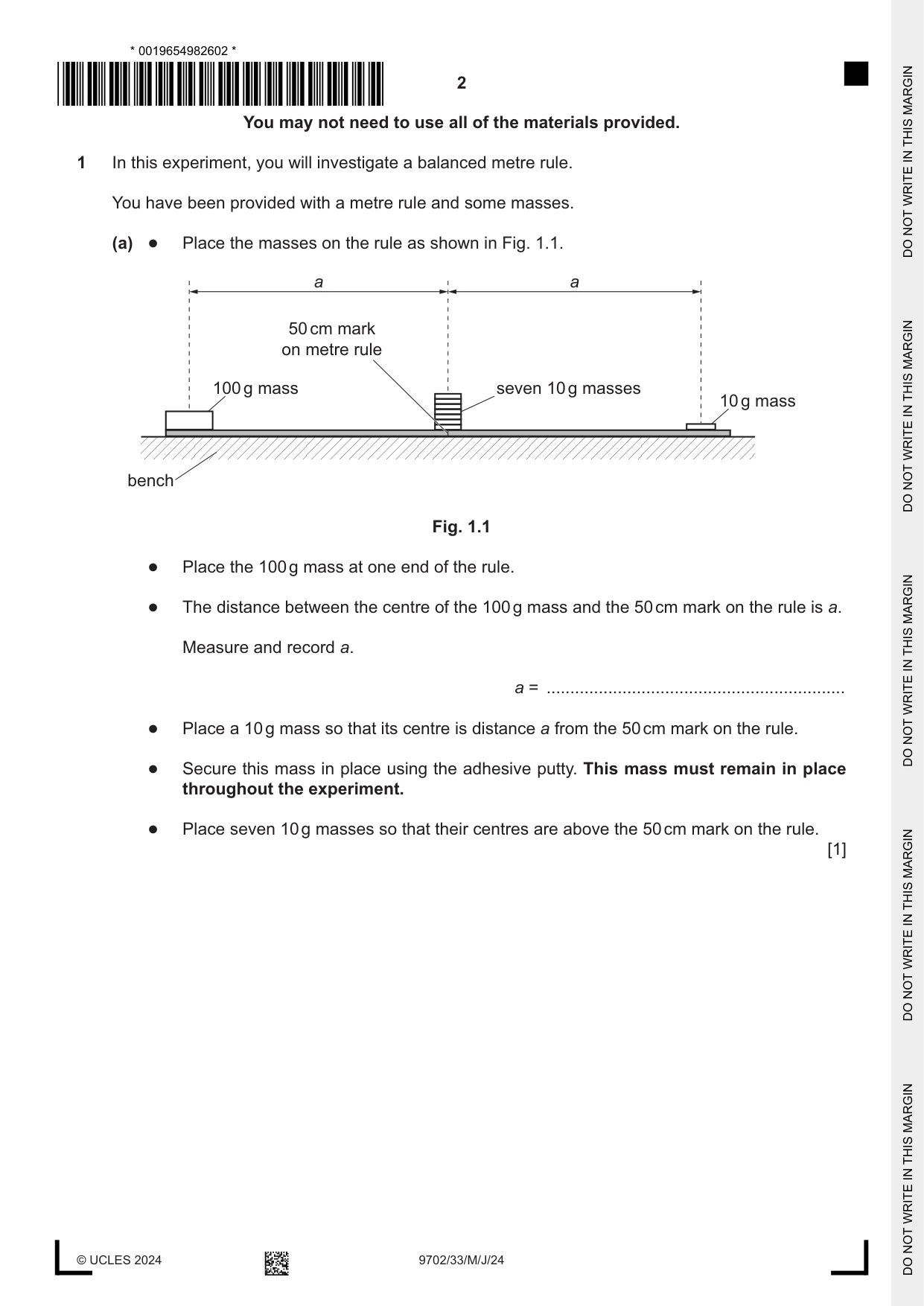
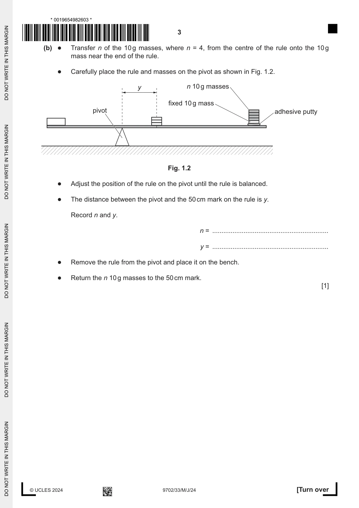
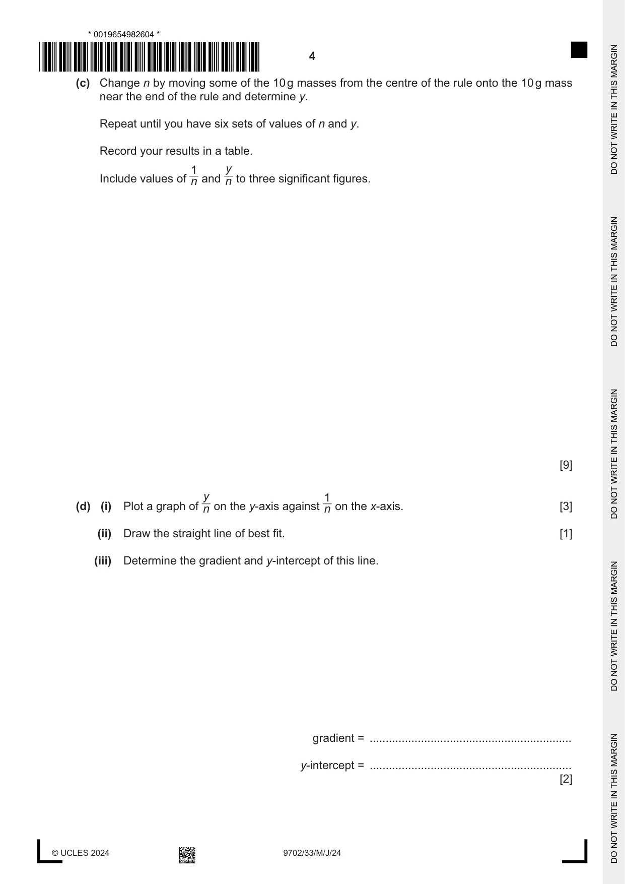
1 In this experiment, you will investigate a balanced metre rule. You have been provided with a metre rule and some masses. (a) ● Place the masses on the rule as shown in Fig. 1.1. a a 50 cm mark on metre rule 100 g mass seven 10 g masses 10 g mass bench Fig. 1.1 ● Place the 100 g mass at one end of the rule. ● The distance between the centre of the 100 g mass and the 50 cm mark on the rule is a. Measure and record a. a = ............................................................... ● Place a 10 g mass so that its centre is distance a from the 50 cm mark on the rule. ● Secure this mass in place using the adhesive putty. This mass must remain in place throughout the experiment. ● Place seven 10 g masses so that their centres are above the 50 cm mark on the rule. [1] (b) ● Transfer n of the 10 g masses, where n = 4, from the centre of the rule onto the 10 g mass near the end of the rule. ● Carefully place the rule and masses on the pivot as shown in Fig. 1.2. y n 10 g masses fixed 10 g mass pivot adhesive putty Fig. 1.2 ● Adjust the position of the rule on the pivot until the rule is balanced. ● The distance between the pivot and the 50 cm mark on the rule is y. Record n and y. n = ............................................................... y = ............................................................... ● Remove the rule from the pivot and place it on the bench. ● Return the n 10 g masses to the 50 cm mark. [1] (c) Change n by moving some of the 10 g masses from the centre of the rule onto the 10 g mass near the end of the rule and determine y. Repeat until you have six sets of values of n and y. Record your results in a table. 1 y Include values of n and n to three significant figures. [9] y 1 (d) (i) Plot a graph of n on the y-axis against n on the x-axis. [3] (ii) Draw the straight line of best fit. [1] (iii) Determine the gradient and y-intercept of this line. gradient = ............................................................... y-intercept = ............................................................... [2] (e) It is suggested that the quantities y and n are related by the equation y P = – Q n n where P and Q are constants. Using your answers in (d)(iii), determine the values of P and Q. Give appropriate units. P = ............................................................... Q = ............................................................... [2] (f) Theory suggests that 9Ma P = 18M + R where M = 10 g and R is the mass of the rule. Determine the value of R. R = ...................................................... g [1] [Total: 20]

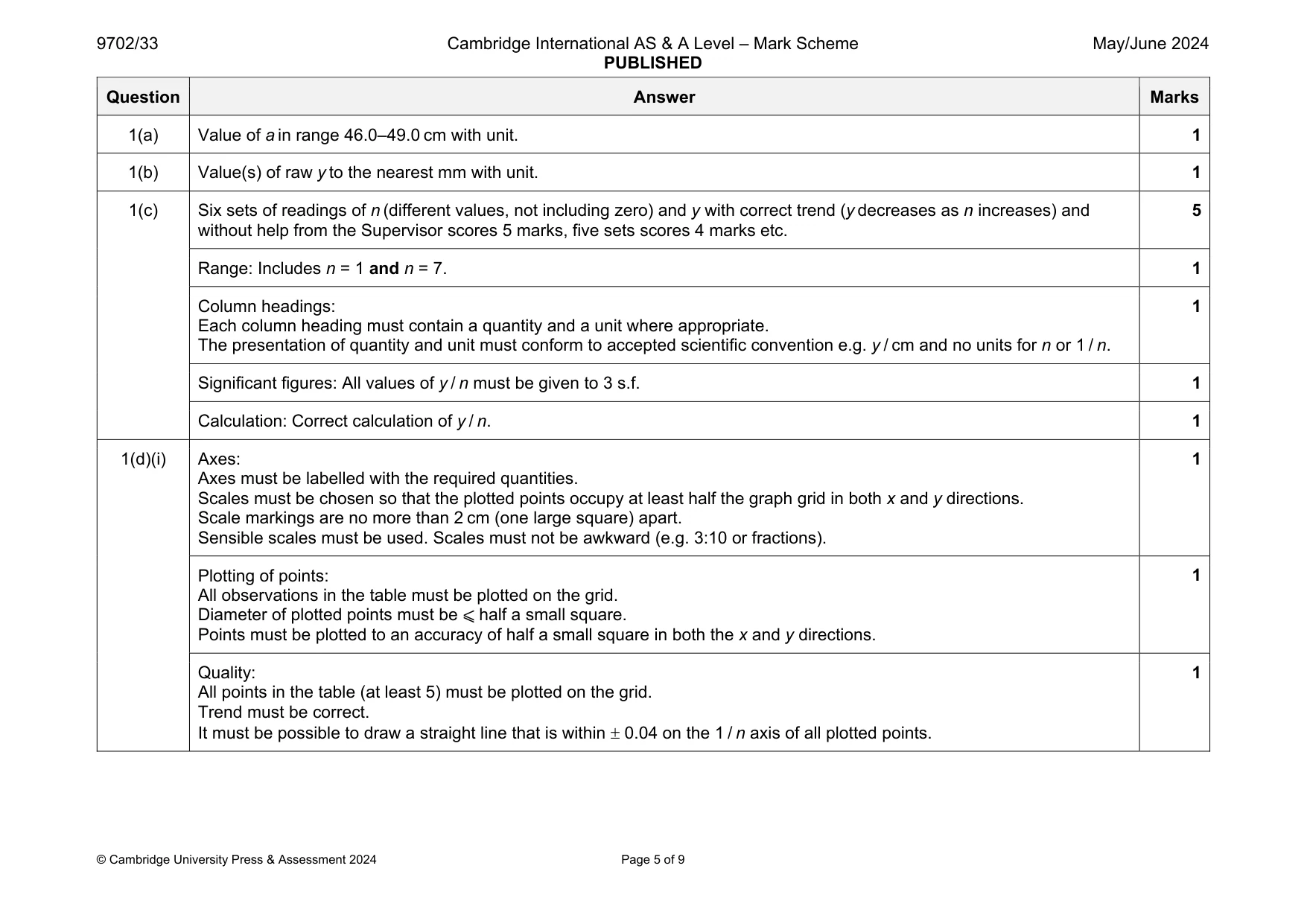
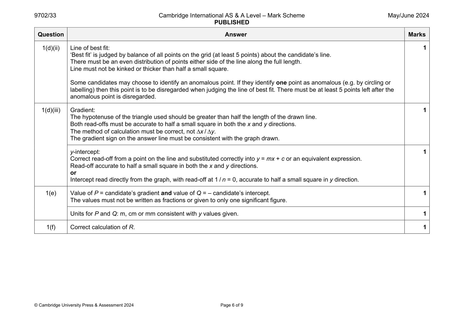
Mark scheme: 1(a) Value of a in range 46.0–49.0 cm with unit. 1 1(b) Value(s) of raw y to the nearest mm with unit. 1 1(c) Six sets of readings of n (different values, not including zero) and y with correct trend (y decreases as n increases) and without help from the Supervisor scores 5 marks, five sets scores 4 marks etc. 5 Range: Includes n = 1 and n = 7. 1 Column headings: Each column heading must contain a quantity and a unit where appropriate. The presentation of quantity and unit must conform to accepted scientific convention e.g. y / cm and no units for n or 1 / n. 1 Significant figures: All values of y / n must be given to 3 s.f. 1 Calculation: Correct calculation of y / n. 1 1(d)(i) Axes: Axes must be labelled with the required quantities. Scales must be chosen so that the plotted points occupy at least half the graph grid in both x and y directions. Scale markings are no more than 2 cm (one large square) apart. Sensible scales must be used. Scales must not be awkward (e.g. 3:10 or fractions). 1 Plotting of points: All observations in the table must be plotted on the grid. Diameter of plotted points must be ⩽ half a small square. Points must be plotted to an accuracy of half a small square in both the x and y directions. 1 Quality: All points in the table (at least 5) must be plotted on the grid. Trend must be correct. It must be possible to draw a straight line that is within  0.04 on the 1 / n axis of all plotted points. 1 Question Answer Marks 1(d)(ii) Line of best fit: ‘Best fit’ is judged by balance of all points on the grid (at least 5 points) about the candidate’s line. There must be an even distribution of points either side of the line along the full length. Line must not be kinked or thicker than half a small square. Some candidates may choose to identify an anomalous point. If they identify one point as anomalous (e.g. by circling or labelling) then this point is to be disregarded when judging the line of best fit. There must be at least 5 points left after the anomalous point is disregarded. 1 1(d)(iii) Gradient: The hypotenuse of the triangle used should be greater than half the length of the drawn line. Both read-offs must be accurate to half a small square in both the x and y directions. The method of calculation must be correct, not x / y. The gradient sign on the answer line must be consistent with the graph drawn. 1 y-intercept: Correct read-off from a point on the line and substituted correctly into y = mx + c or an equivalent expression. Read-off accurate to half a small square in both the x and y directions. or Intercept read directly from the graph, with read-off at 1 / n = 0, accurate to half a small square in y direction. 1 1(e) Value of P = candidate’s gradient and value of Q = – candidate’s intercept. The values must not be written as fractions or given to only one significant figure. 1 Units for P and Q: m, cm or mm consistent with y values given. 1 1(f) Correct calculation of R. 1

More questions on Turning effects of forces

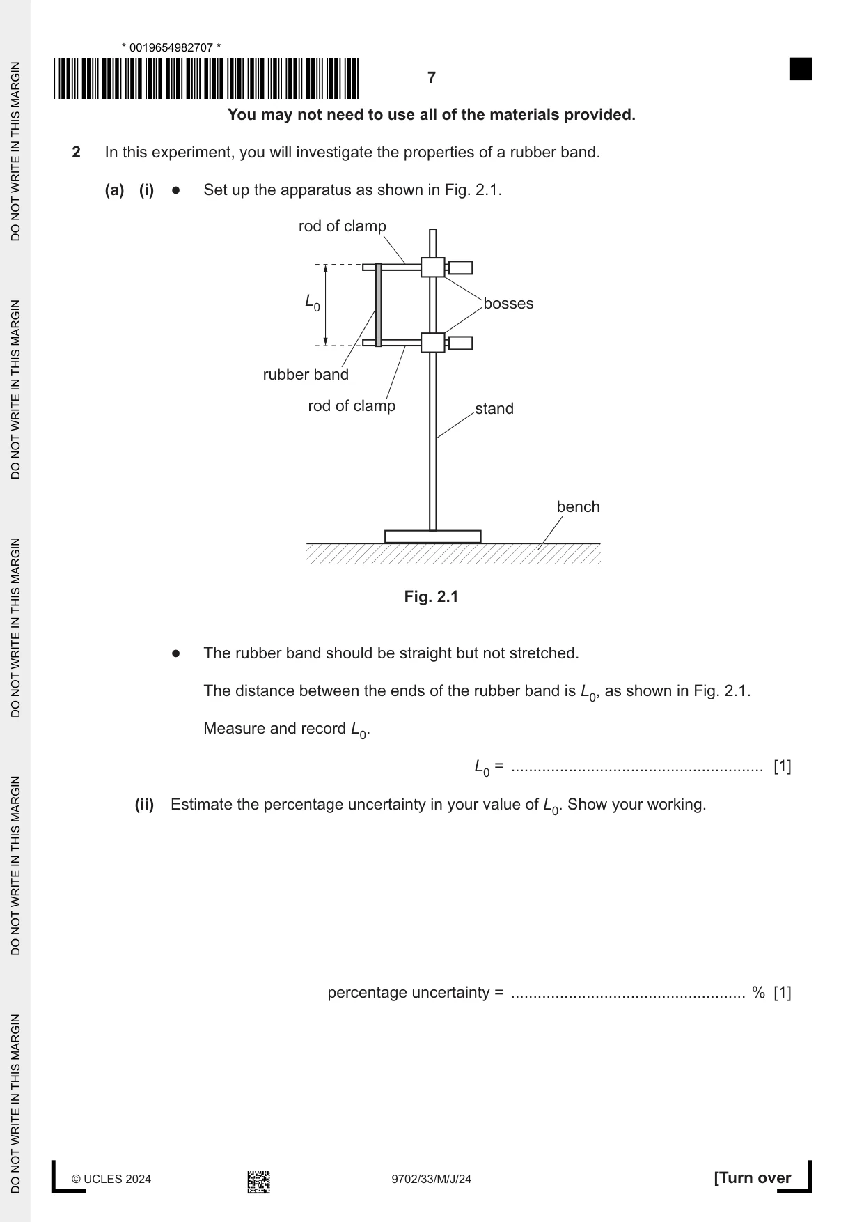
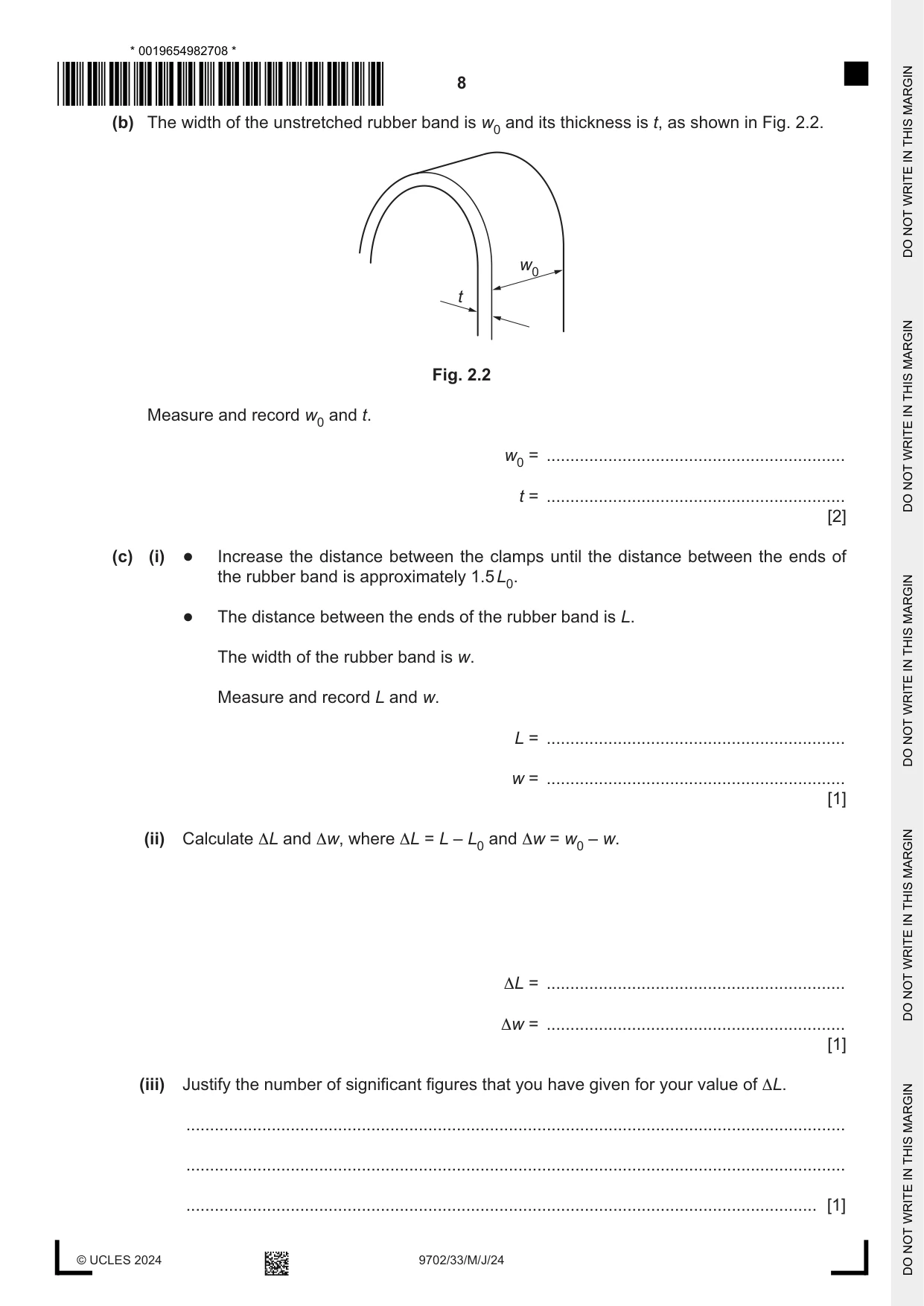
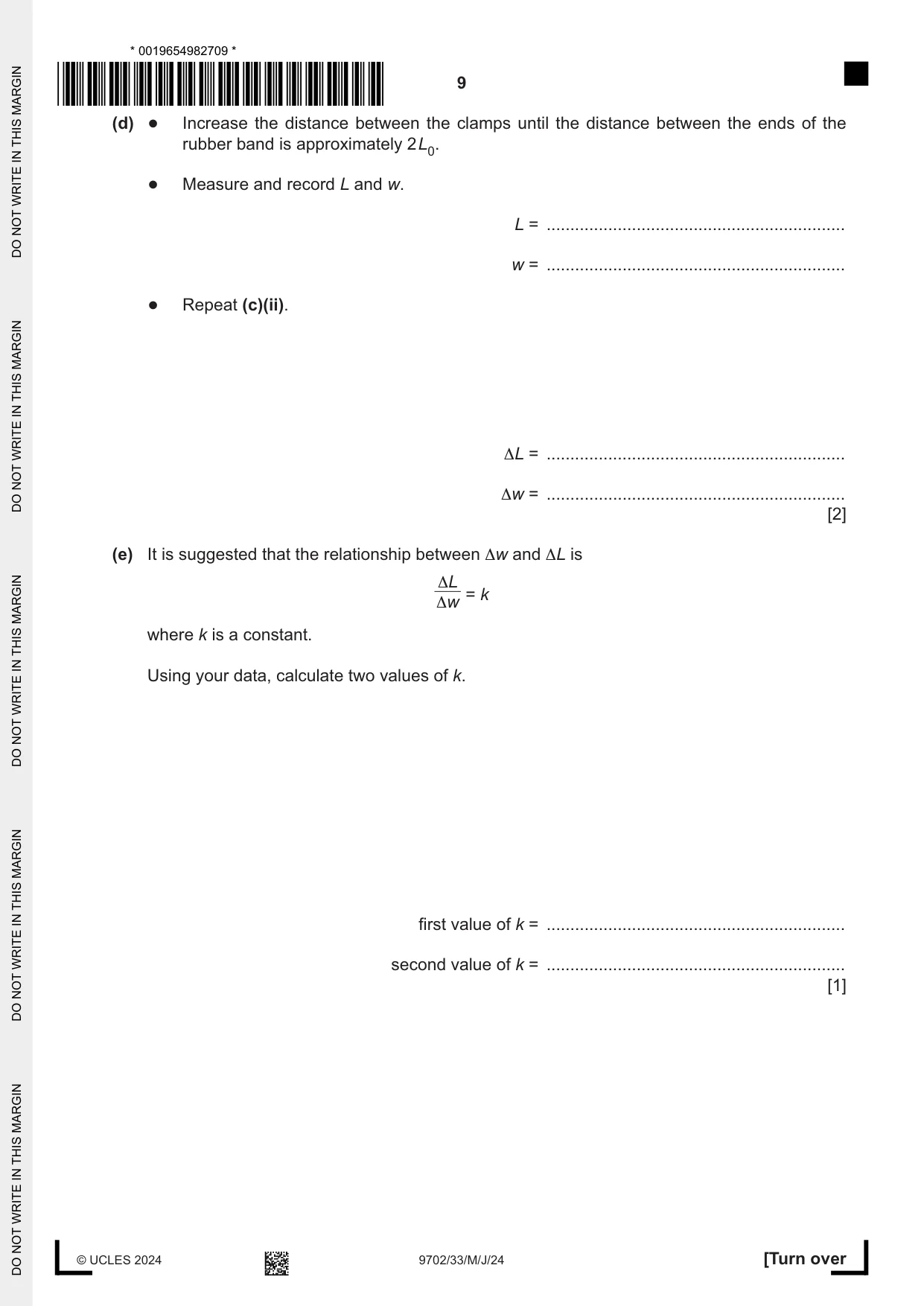
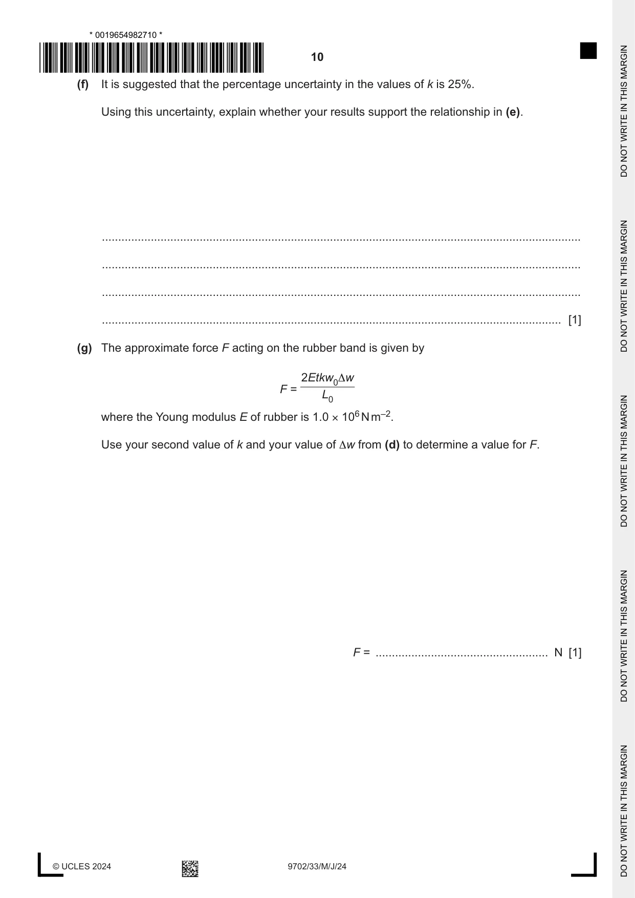
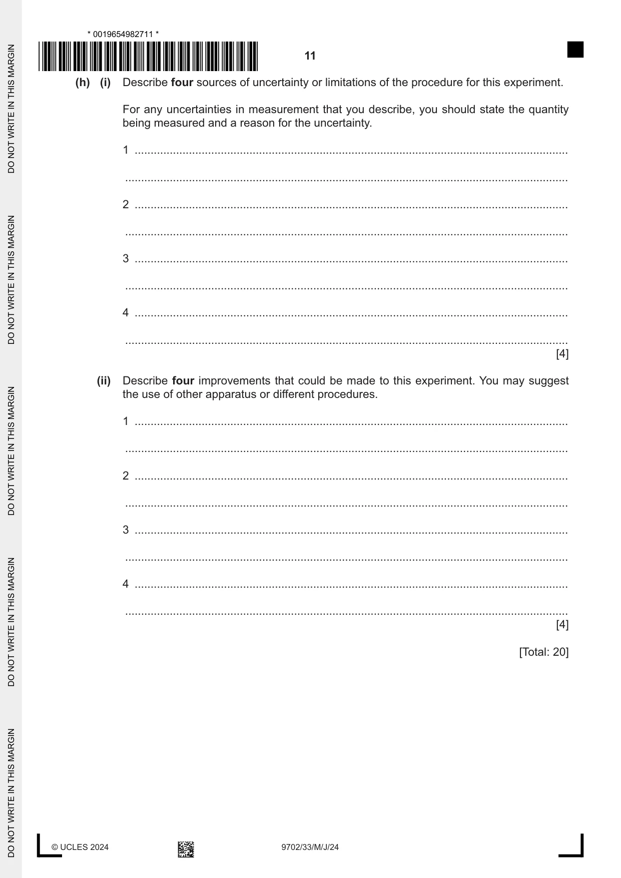
2 In this experiment, you will investigate the properties of a rubber band. (a) (i) ● Set up the apparatus as shown in Fig. 2.1. rod of clamp L0 bosses rubber band rod of clamp stand bench Fig. 2.1 ● The rubber band should be straight but not stretched. The distance between the ends of the rubber band is L0, as shown in Fig. 2.1. Measure and record L0. L0 = ......................................................... [1] (ii) Estimate the percentage uncertainty in your value of L0. Show your working. percentage uncertainty = ..................................................... % [1] (b) The width of the unstretched rubber band is w0 and its thickness is t, as shown in Fig. 2.2. w0 t Fig. 2.2 Measure and record w0 and t. w0 = ............................................................... t = ............................................................... [2] (c) (i) ● Increase the distance between the clamps until the distance between the ends of the rubber band is approximately 1.5 L0. ● The distance between the ends of the rubber band is L. The width of the rubber band is w. Measure and record L and w. L = ............................................................... w = ............................................................... [1] (ii) Calculate ΔL and Δw, where ΔL = L – L0 and Δw = w0 – w. ΔL = ............................................................... Δw = ............................................................... [1] (iii) Justify the number of significant figures that you have given for your value of ΔL. ........................................................................................................................................... ........................................................................................................................................... ..................................................................................................................................... [1] (d) ● Increase the distance between the clamps until the distance between the ends of the rubber band is approximately 2 L0. ● Measure and record L and w. L = ............................................................... w = ............................................................... ● Repeat (c)(ii). ΔL = ............................................................... Δw = ............................................................... [2] (e) It is suggested that the relationship between Δw and ΔL is ΔL = k Δw where k is a constant. Using your data, calculate two values of k. first value of k = ............................................................... second value of k = ............................................................... [1]

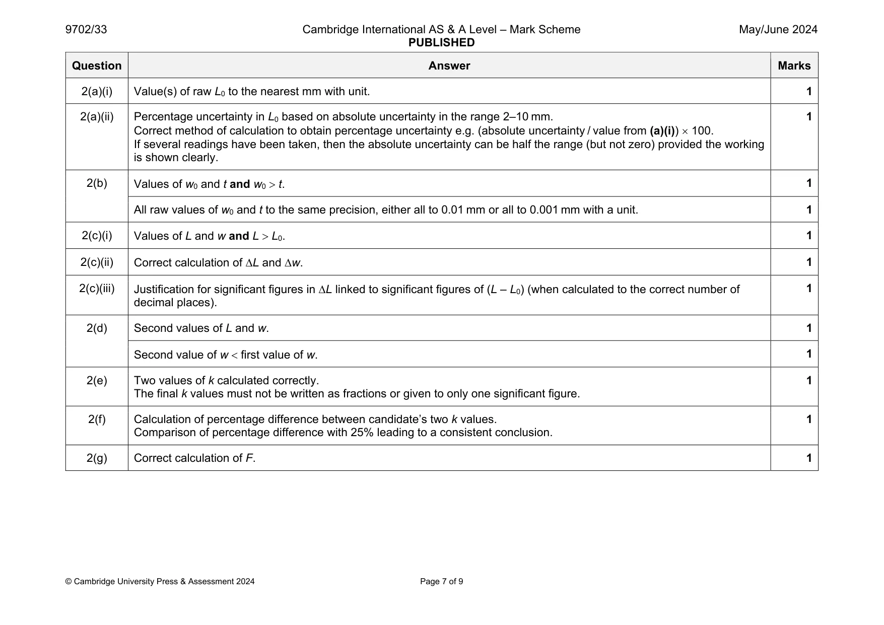
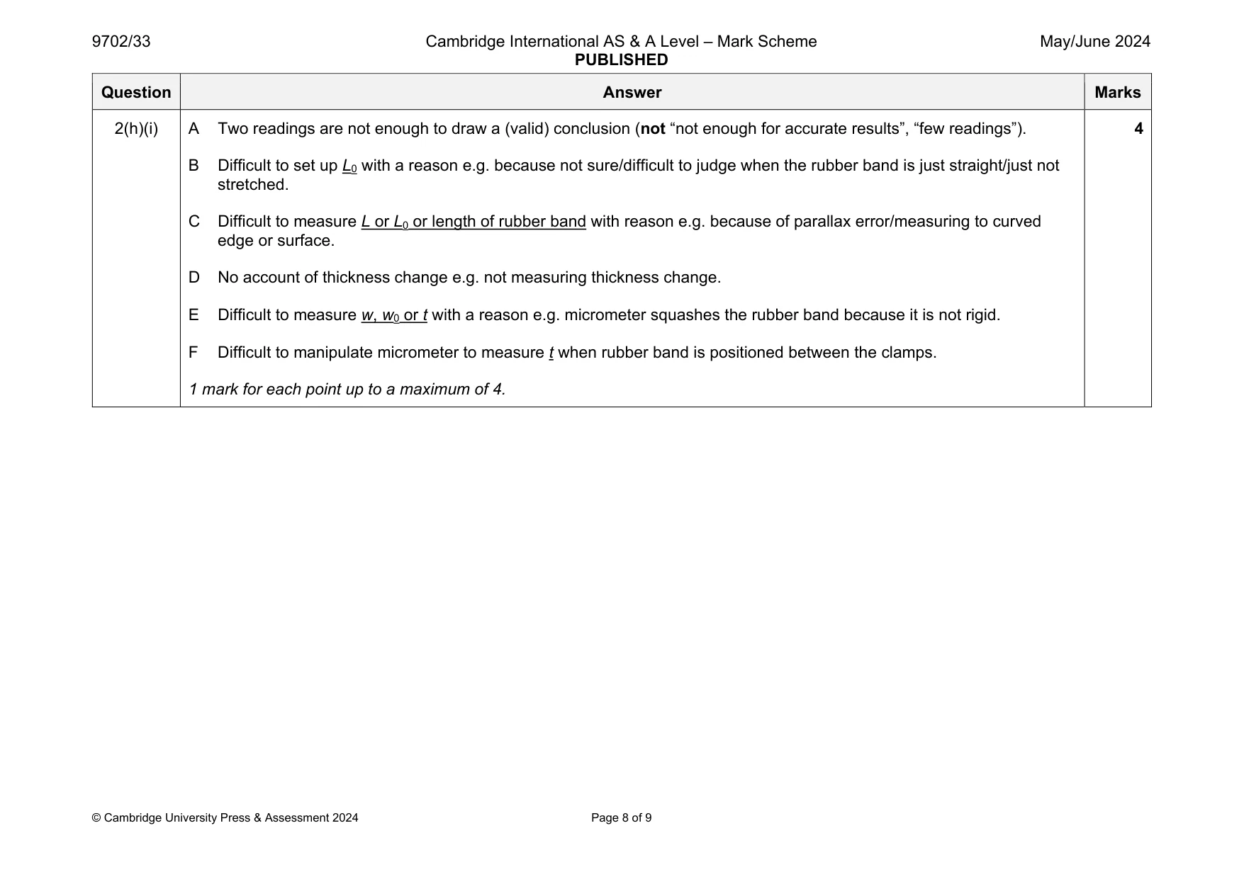
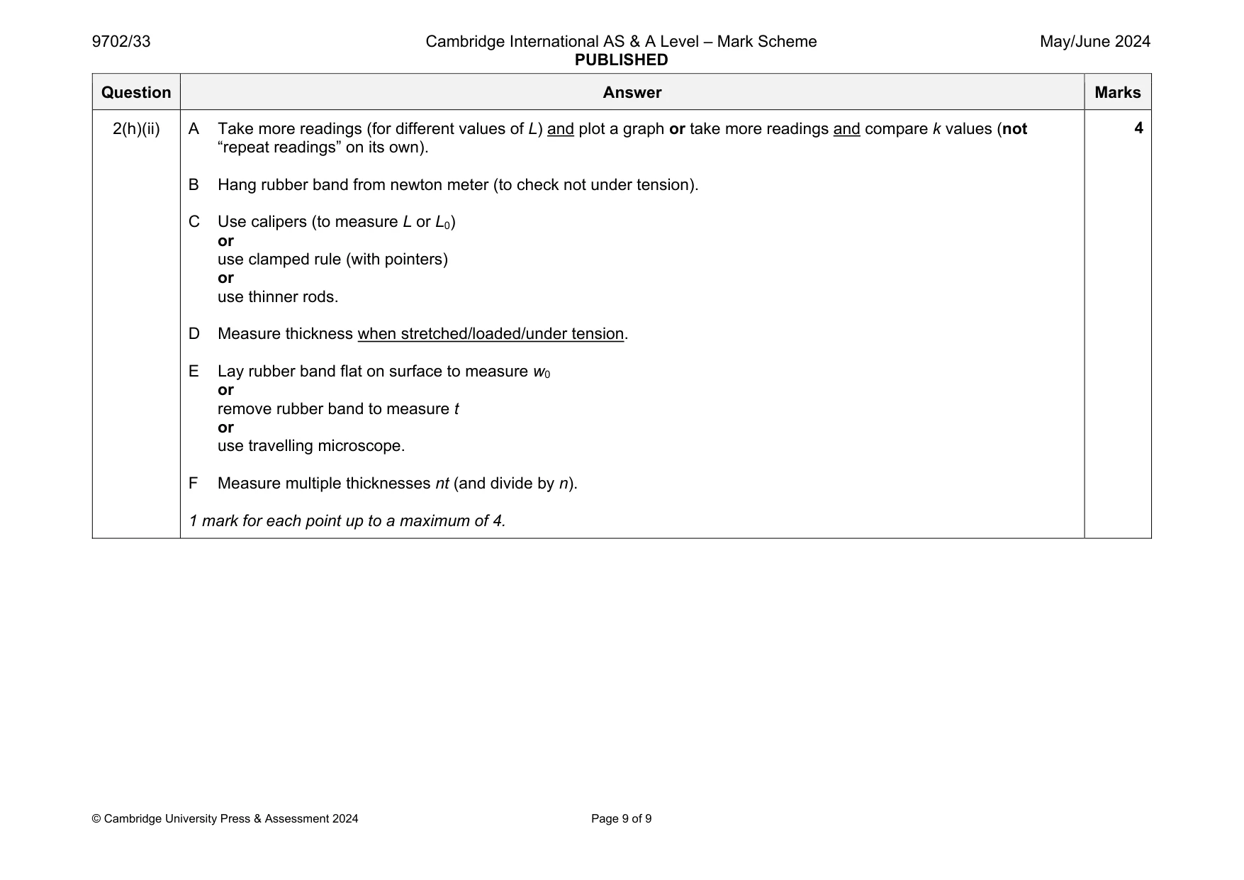
Mark scheme: 2(a)(i) Value(s) of raw L0 to the nearest mm with unit. 1 2(a)(ii) Percentage uncertainty in L0 based on absolute uncertainty in the range 2–10 mm. Correct method of calculation to obtain percentage uncertainty e.g. (absolute uncertainty / value from (a)(i))  100. If several readings have been taken, then the absolute uncertainty can be half the range (but not zero) provided the working is shown clearly. 1 2(b) Values of w0 and t and w0  t. 1 All raw values of w0 and t to the same precision, either all to 0.01 mm or all to 0.001 mm with a unit. 1 2(c)(i) Values of L and w and L  L0. 1 2(c)(ii) Correct calculation of L and w. 1 2(c)(iii) Justification for significant figures in L linked to significant figures of (L – L0) (when calculated to the correct number of decimal places). 1 2(d) Second values of L and w. 1 Second value of w  first value of w. 1 2(e) Two values of k calculated correctly. The final k values must not be written as fractions or given to only one significant figure. 1 2(f) Calculation of percentage difference between candidate’s two k values. Comparison of percentage difference with 25% leading to a consistent conclusion. 1 2(g) Correct calculation of F. 1 Question Answer Marks 2(h)(i) A Two readings are not enough to draw a (valid) conclusion (not “not enough for accurate results”, “few readings”). B Difficult to set up L0 with a reason e.g. because not sure/difficult to judge when the rubber band is just straight/just not stretched. C Difficult to measure L or L0 or length of rubber band with reason e.g. because of parallax error/measuring to curved edge or surface. D No account of thickness change e.g. not measuring thickness change. E Difficult to measure w, w0 or t with a reason e.g. micrometer squashes the rubber band because it is not rigid. F Difficult to manipulate micrometer to measure t when rubber band is positioned between the clamps. 1 mark for each point up to a maximum of 4. 4 Question Answer Marks 2(h)(ii) A Take more readings (for different values of L) and plot a graph or take more readings and compare k values (not “repeat readings” on its own). B Hang rubber band from newton meter (to check not under tension). C Use calipers (to measure L or L0) or use clamped rule (with pointers) or use thinner rods. D Measure thickness when stretched/loaded/under tension. E Lay rubber band flat on surface to measure w0 or remove rubber band to measure t or use travelling microscope. F Measure multiple thicknesses nt (and divide by n). 1 mark for each point up to a maximum of 4. 4

More questions on Physical quantities